A GRID-Based Spatial Interpolation Method as a Tool Supporting Real Estate Market Analyses

Abstract

The spatial distribution of prices is closely linked with the urban real estate market. Property prices are one of the key indicators of economic activity because they influence economic decisions. Decision-makers and consumers often need information about the spatial distribution of prices, but spatial-temporal analyses of the real estate market are based on the prices quoted in different locations across years (epochs). Due to this idiosyncrasy, the resulting datasets are dispersed (different across years) and difficult to compare. For this reason, the existing interpolation methods are not always effective in analyses of the real estate market. A different approach to interpolating real estate prices that supports the generation of continuous interpolated surfaces while maintaining the values of measurement points is thus needed. This paper proposes a method for replacing dispersed spatial data with a regular GRID structure. The GRID structure covers the measured object with a regular network of nodes, which supports uniform interpolation at every point of the analyzed space and a comparison of interpolation models in successive epochs (years). The proposed method was tested on a selected object. The results indicate that the GRID structure can be used in analyses of highly complex real estate markets where input data are incomplete, irregular and dispersed.

1. Introduction

The market of residential property is defined as “geographic areas where the price per unit of housing quantity (defined using some index of housing characteristics) is constant” [1]. The spatial distribution of prices is closely linked with the real estate market. Property prices are one of the key indicators of economic activity because they influence economic decisions and constitute vital statistical data. Decision-makers and consumers often need information about the spatial distribution of prices. Property transactions can be represented by points (in simple terms), and they are highly differentiated, which significantly impairs analyses of changes in local markets over time [2]. The hedonic regression method and the repeat-sales method are most frequently used in real estate market analyses [3,4,5,6,7,8,9,10,11]. The emergence of geographic information system (GIS) tools contributed to the development of surface models with the use of spatial interpolation methods (geostatistical methods) [12,13,14,15,16,17]. According to Chou [18], spatial interpolation relies on two fundamental assumptions: The surface of the price variable is continuous (therefore, the value can be estimated at every location), and the price variable is spatially dependent (the value in a specific location is related to the values in surrounding locations). The presence of spatial correlations between prices resulting from neighborhood effects has been observed by many authors [3,19,20,21,22], and it supports price analyses with the use of various interpolation methods.

Spatial information systems (SIS) are used to describe, analyze, explain, interpret and predict different phenomena in physical space. Spatial data visualization methods also support analyses of values which can be localized in a spatial reference system [23,24]. Databases are introduced to obtain information from various measurement epochs, which supports the analysis of changes in data over time. A spatial information system is transformed into a dynamic spatial information system (DSIS) when the time dimension is taken into account. The DSIS can be used to analyze physical or economic data in a given period of time to provide a comprehensive view of the examined phenomena [25,26]. The processing capabilities of IT systems have to increase to accommodate the continued increase in the volume of data that are accumulated in successive epochs. There is an ongoing search for new methods of analyzing and interpreting data that can be localized in a land information system (LIS) or a geographic information system (GIS). Digital solutions from various data processing domains are combined to develop new methods in spatial data mining (SDM) [27,28,29].

The aim of this study was to evaluate the applicability of a GRID structure for surface interpolation in an analysis of the dynamics of change in the real estate market. In this approach, the GRID structure constitutes a regular network of squares whose values in nodes (distributed in the corners of squares where the size of the base side can be freely adjusted) are determined by interpolation algorithms based on measurement points (real estate price) in the proximity of each node. The application of a GRID structure in spatiotemporal analyses is justified by the characteristic attributes of the real estate market. In the referenced literature, a spatiotemporal analysis of the real estate market relies on the prices acquired in different locations in successive years (measurement epochs). Due to this idiosyncrasy, the resulting datasets are dispersed (different across years) and difficult to compare. The above applies particularly to the interpolation of class intervals and their comparison on a common scale based on a triangulated irregular network (TIN) where successive nodes of the triangulated grid represent the prices obtained directly from the real estate market. The use of direct measurements (prices) often makes it impossible to model the analyzed area with a uniform triangulated network. Triangles have sides of different length, which disrupts the interpolation of isolines forming class intervals with the same precision across the entire area (Figure 4b,c). As a result, the differences between epochs cannot be accurately determined in areas with a low density of the measured data. A high density of data, on the other hand, obstructs analyses of extreme prices. For this reason, TIN is not always directly recommended for spatial analyses. Areas where data were acquired in different periods of time (in different epochs) are particularly difficult to compare. In selected measurement points, data are not available for all epochs; therefore, selected locations cannot be accurately compared.

Those limitations create the need for different price interpolation methods on the real estate market. This study proposes innovative solutions for real estate market analysis, and the presented methods improve the quality of the analysis. The article discusses a method for replacing dispersed spatial data with a regular GRID structure. The solutions based on a GRID structure support:

-

reduction of excess information,

-

reduction or elimination of redundant information,

-

reduction of the volume of datasets stored in databases,

-

compensation for measurement errors,

-

reduction of the number of points describing a surface,

-

stepless regulation of grid resolution and adaptation of grid resolution to the morphology of the analyzed surface,

-

increasing node resolution on the examined surface for greater accuracy,

-

performance of analyses in consecutive measurement epochs at various locations with different density of measurement points,

-

performance of comparative analyses at the same node points which are determined mathematically,

-

acceleration of data modeling and visualization,

-

optimization of algorithms for faster processing of digital data,

-

simplification of directional (profile-related) data modeling and analysis,

-

greater clarity and transparency of the spatial organization of data,

-

precise arrangement and organization of the topological structure of stored data,

-

more convenient access to the required information in the data exploration process,

-

convenient and efficient data archiving,

-

multi-epoch archiving and modeling data for a specific time period,

-

higher efficiency of spatial data processing in real-time,

-

higher efficiency of database management systems (DBMS) [30],

-

acceleration of spatial data mining (SDM) [27,29],

-

acceleration of data transfer between spatial information systems (SIS) [31],

-

increasing the speed of access to data in internet spatial data servers (ISDS) [32],

-

simplification of the structure of recording and reading data in spatial database (SDB) models [33,34],

-

acceleration of spatial online application processing (SOLAP) [35],

-

increasing the data processing capacity of dynamic SIS (DSIS) [26].

The above attributes justify the comprehensive use of the GRID structure in various stages of data processing in the proposed methodology.

The object and the spatial range of the study, and the method of preparing input data are discussed, price interpolations based on TIN and GRID surfaces are compared, and selected statistical indicators are interpreted in successive sections of the article. The principles for selecting interpolation algorithms and the resolution of the GRID structure are presented in the Results section in view of the location of measurement points in the analyzed area. Interpolation surfaces were also compared in different measurement epochs (years), and the values of numerical indicators describing changes over time were interpreted.

2. Materials and Methods

2.1. Subject Matter and Spatial Range of Analysis

This study analyzed the prices of apartments traded in 2005–2014 in the city of Olsztyn (Poland) in two residential estates. The accumulated data were classified into 10 measurement epochs. The average price of apartments (PLN/m²; PLN–Polish zloty) traded in each epoch constituted the input data for further analyses. The average price was assigned to the location of the investigated object (building) in the adopted reference system (WGS 84 Web Mercator).

The analyzed dataset was highly homogeneous in terms of the following factors:

-

the examined housing resources were similar (same construction technology and year of construction, similar renovation and insulation solutions, which led to a similar degree of technical and functional wear),

-

the examined resources were managed by the same administrator,

-

the analyzed estates had a compact structure,

-

market demand was stable,

-

the analyzed estates accounted for 16% of housing resources in Olsztyn,

-

changes in apartment prices over time were similar to the trends observed in Olsztyn and across Poland,

-

the evaluated property was narrowed down to apartments with an average floor area of 40–60 m².

An analysis of the dataset covering 2005 to 2014 revealed that the local property market developed dynamically in 2005–2007 and that prices rose rapidly and peaked in 2007. Market growth was stalled in successive years, and the steady drop in prices was deepened in 2011–2012.

The evaluated area was analyzed in detail based on interpolated surfaces generated with the use of a GRID structure.

2.2. Preparation of Input Data

To develop a single-level database, every data record was written in three data fields. The address of the building containing the analyzed apartment was represented with two geographic coordinates (e.g., 53.737152N, 20.489984E). The coordinates of a measurement point were determined in the geometric center of the building where the traded apartment was located. The price (P) of the traded apartment was the third data field. If several apartments were traded in the same building, the arithmetic mean of their prices was used in the analysis. The geographic coordinates of a measurement point (differing in the third decimal place) were rescaled to 1,000,000:1 to visualize spatial data in a homogeneous system. The price per unit, which was entered in the third data field, was not modified. Data for further analyses were reduced to a single-level database with identical records comprising fields N, E and P. A rectangle with coordinates N: 53.735900–53.746248 and E: 20.489660–20.520569 was drawn over all datasets to produce identically sized areas in all epochs. In the resulting datasets, the number and location of data differed across the analyzed years (year–number of data: 2005–80; 2006–108; 2007–83; 2008–115; 2009–111; 2010–135; 2011–127; 2012–89; 2013–96; 2014–97).

2.3. Methods

2.3.1. Price Interpolation in the TIN Surface Model

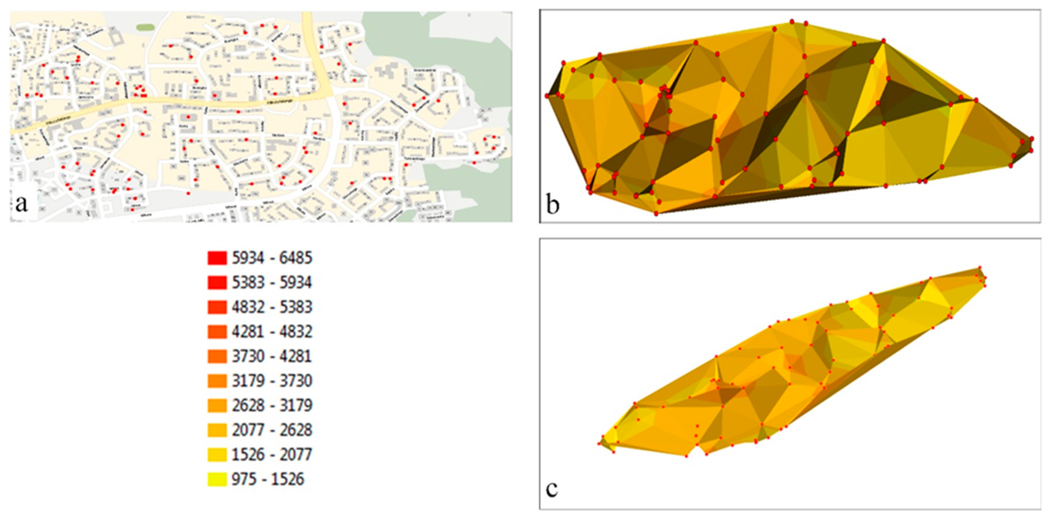
In the presented example, the price data for 2005 create a set of dispersed points characterized by varied density in different segments of the analyzed area (Figure 1a). A similar pattern is observed in the remaining epochs, where the locations of measurement points in successive years do not overlap.

The minimum and maximum values of data for the entire period of analysis (2005–2014) were set at min = PLN 975/m² and max = PLN 6485/m² to represent all property prices in a homogeneous spatial system. The obtained values were then divided into 10 class intervals. The interpolated property prices were modeled with a TIN surface where successive nodes represented direct market prices (Figure 1b,c). The analyzed values were sampled in different locations in successive years, and they formed dispersed sets that were difficult to compare. As a result, the differences between epochs could not be accurately determined in areas characterized by low data density. A high density of data, on the other hand, obstructed analyses of extreme prices. The use of direct measurements (prices) often makes it impossible to model the analyzed area with a uniform triangulated network. Triangles have sides of different lengths, which disrupts the interpolation of isolines forming class intervals with the same precision across the entire area (Figure 1b,c). For this reason, TIN is not always directly recommended for spatial analyses. In some measurement points, data are not available for all epochs; therefore, selected locations cannot be accurately compared.

2.3.2. Price Interpolation in a GRID Surface Model

A regular network of nodes forming a GRID type structure can be used to guarantee that points with selected values are uniformly distributed across the analyzed area [36,37,38]. The grid can be developed based on regular shapes, but a regular network of squares with identical sides is most often used. The horizontal location of grid nodes is defined by a pair of coordinates XY (in this case: NE) which can be mapped in the same location for every epoch. The third coordinate is determined with the use of measurement points (in this case: apartment prices) located near every node of the grid of squares. The value in each node is determined by interpolation with a selected algorithm.

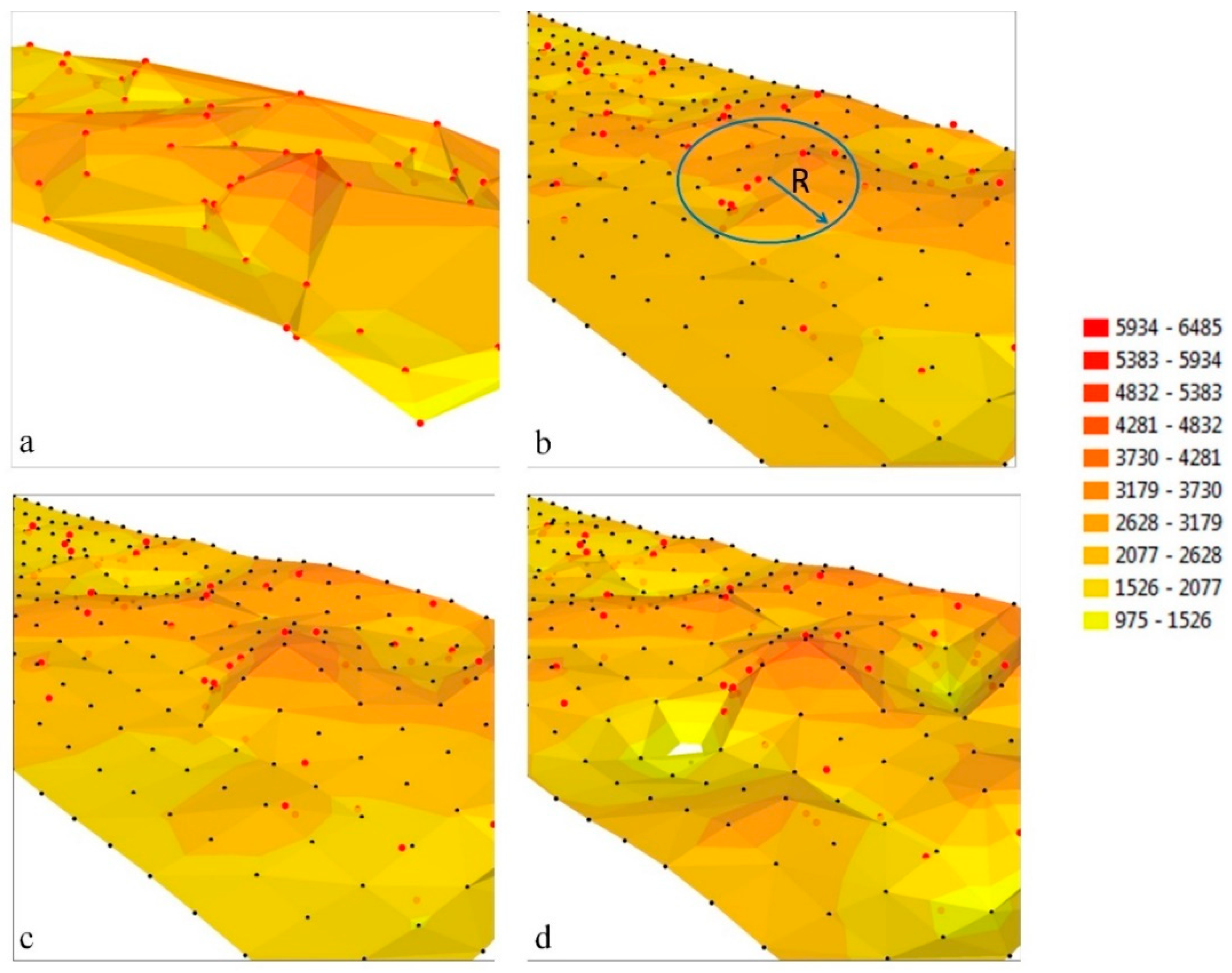
The same fragment of space represented by differently generated surfaces is shown in Figure 2. The surface generated with direct measurements is a TIN structure, and it is based on a triangulated irregular network (Figure 2a). It is characterized by irregularly distributed measurement points that are responsible for the irregular shape of the generated surface. In GRID structures (Figure 2b–d), the nodes creating the surface model are found in the corners of regularly distributed squares, and their location on plane XY is controlled by a constant distance interval in both directions of the axis. The interval determines the resolution of a GRID structure which can be freely regulated. Unlike a TIN structure (Figure 2a), a GRID structure (Figure 2b–d) models the analyzed object with a regular node network, which supports uniform interpolation at every point on the analyzed surface.

2.3.3. Statistical Indicators

Interpolated surfaces can be generated from an identical number of points in each epoch when irregularly distributed measurement data are replaced with a regular network of nodes in a GRID structure. A nonhomogeneous dataset from each epoch can be transformed into a homogeneous dataset (with an equal number of attributes) for an identical number of nodes with the same resolution. An identical number of data in each year supports the comparison of successive epochs with the use of statistical indicators. Selected epochs can be compared against the average value for a given period or an average value computed for a specific period. The values determined in each node can be used in statistical calculations. Statistical analyses can be performed with the use of selected indicators [39,40,41]. Statistical attributes can include the difference in the values assigned to every node in a GRID structure (independently for each epoch) and the overall arithmetic mean where weights were assigned to the number of measurements in each epoch (Equation (1)). This approach can be used to compare the accuracy of the interpolated surfaces generated based on GRID nodes with the actual measurement data.

$$\overline{x}=\frac{{\sum }_{i=1}^k{x}_i{n}_i}{{\sum }_{i=1}^k{n}_i},$$

(1)

where:

• k—number of epochs,
• xi—ordinary arithmetic mean of values in a given epoch,
• ni—number of data (the number of attributes is equal to the number of measurements) in a given epoch.

The average difference in the values of successive nodes can be adopted as the ordinary average for each epoch (Equation (2)).

$$x=\frac{{\sum }_{i=1}^n(w_i-\overline{x})}{n},$$

(2)

where:

• n—number of data (the number of attributes is equal to the number of nodes) in an epoch,
• w_i—values assigned to nodes in a given epoch,
• $\overline{x}$—arithmetic mean of data from all epochs (Equation (1)).

Successive epochs can be compared with the use of indicators describing the compared surfaces based on a single value for every epoch (Equation (3)). Standard deviation (Equation (2)) and RMS (Equation (4)) were used in the presented example. Standard deviation in Equation (3) was calculated to evaluate the variation of an attribute within a set. The value of an attribute in a set was described by the value assigned to different nodes in a given epoch, and the differences between node values and the ordinary average value for each epoch were calculated. This approach supports a comparison of differences in each epoch (variation within each set) with other epochs and with the average for a given period. In the presented examples, the higher the standard deviation, the greater the variations in the interpolated surfaces and, consequently, the greater the differences in property prices in a given epoch. Standard deviation can also be compared in successive epochs to determine the extent to which a given epoch deviates from the average for the investigated period.

$$s=\sqrt{\frac{1}{n-1}{\sum }_{i=1}^n{(w_i-x)}^2},$$

(3)

where:

• n—number of data (the number of attributes is equal to the number of nodes) in a given epoch,
• wi—values assigned to nodes in a given epoch,
• x—ordinary average of differences in node values (Equation (2)).

The goodness of fit between the interpolated surfaces and the reference surface is compared with the RMSE. In the presented example, the reference surface comprises the surfaces of a plane created by the values of the overall average (Equation (1)). Those values were assigned to every node used in calculations. The lower the RMSE, the better the fit between the evaluated surfaces. In the presented example, the lower the RMSE, the closer the property prices are to the average for the analyzed period.

$$RMS=\sqrt{\frac{1}{n}{\sum }_{i=1}^n{(w_i-\overline{x})}^2},$$

(4)

where:

• n—number of data (the number of attributes is equal to the number of nodes) in a given epoch,
• w_i—values assigned to nodes in a given epoch,
• $\overline{x}$—overall arithmetic mean for data from all epochs (Equation ((1)).

3. Results

3.1. Selection of Interpolation Algorithm

The selection of an interpolation algorithm is an important stage in analyses deploying a GRID structure. In the presented example, the interpolation surfaces for analysis were generated with three algorithms: inverse distance to a power, kriging and radial basis function. This approach supported a comparison of interpolation results and the selection of the optimal solution for further analyses.

During the generation of GRID structures, the values in interpolation nodes are computed with the use of measurement points located near the mapped node within a given search radius R (Figure 2b). The size of the radius is determined relative to the resolution of the node network, and an interpolation algorithm is selected to control the degree of generalization of the developed surface [42,43,44,45,46]. The shape of the interpolated surface generated based on GRID nodes can differ depending on the applied algorithm and its processing parameters. The choice of interpolation algorithm is determined by many factors, in particular, the distribution of measurement points, the resolution of the generated structure, the number of searched measurement points within a given radius, their location in sectors surrounding the node and the parameters of an interpolation algorithm [45,46,47,48]. In Figure 2, interpolation results are represented by the surfaces generated in the GRID model with inverse distance to a power (IDP), kriging (K) and radial base function (RBF) algorithms. The root mean square error of the interpolated surface to the TIN surface was calculated for all measurement points (Equation (4)) to select the best interpolation algorithm. The least satisfactory fit was obtained for the surface generated by the IDP algorithm. The surface models generated with K and RBF algorithms produced a similar fit, and local extrema were noted in the RBF model (Figure 2d). The most accurate GRID models were generated by algorithm K, and this algorithm was used to create interpolation surfaces in all epochs.

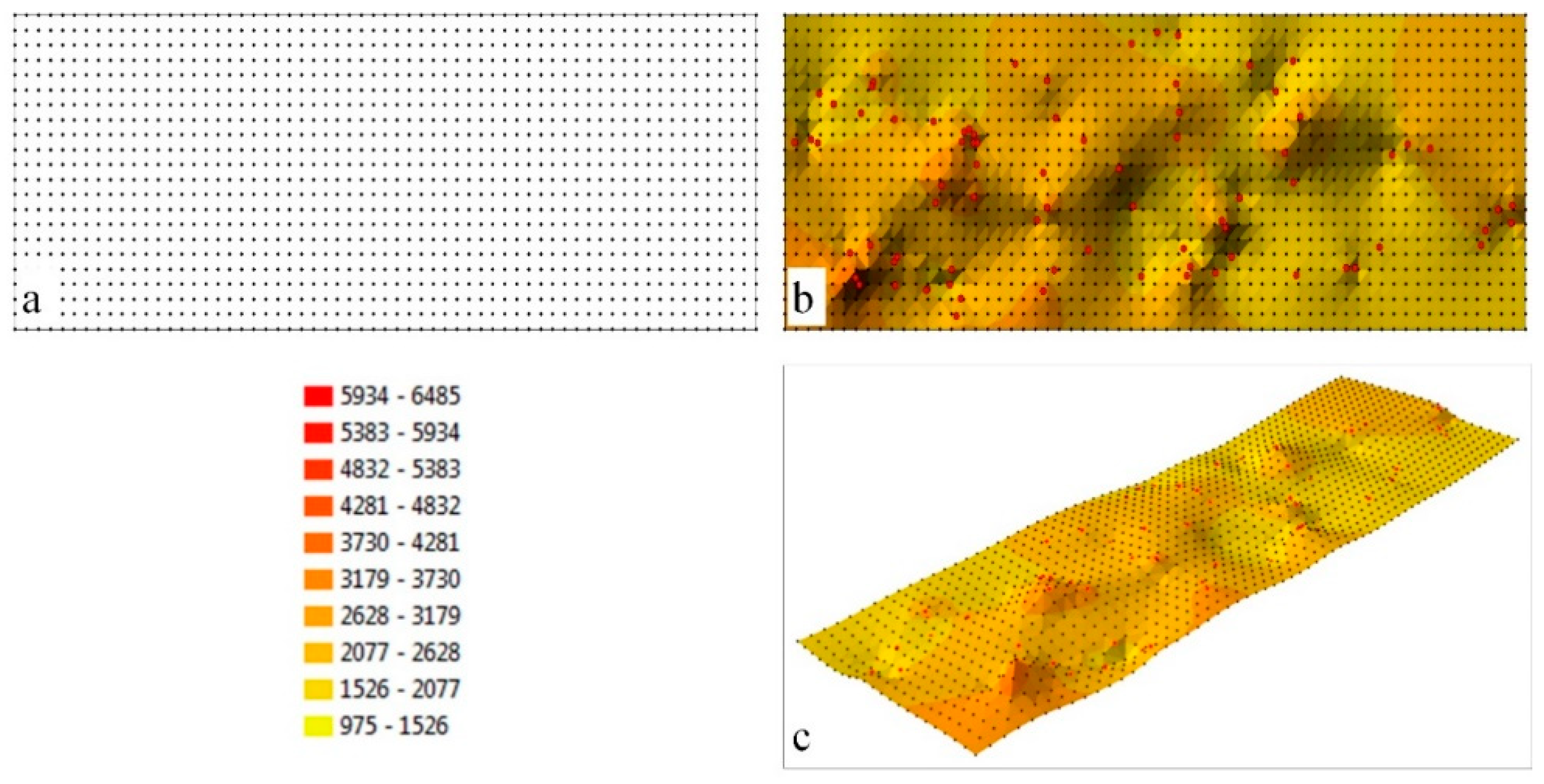
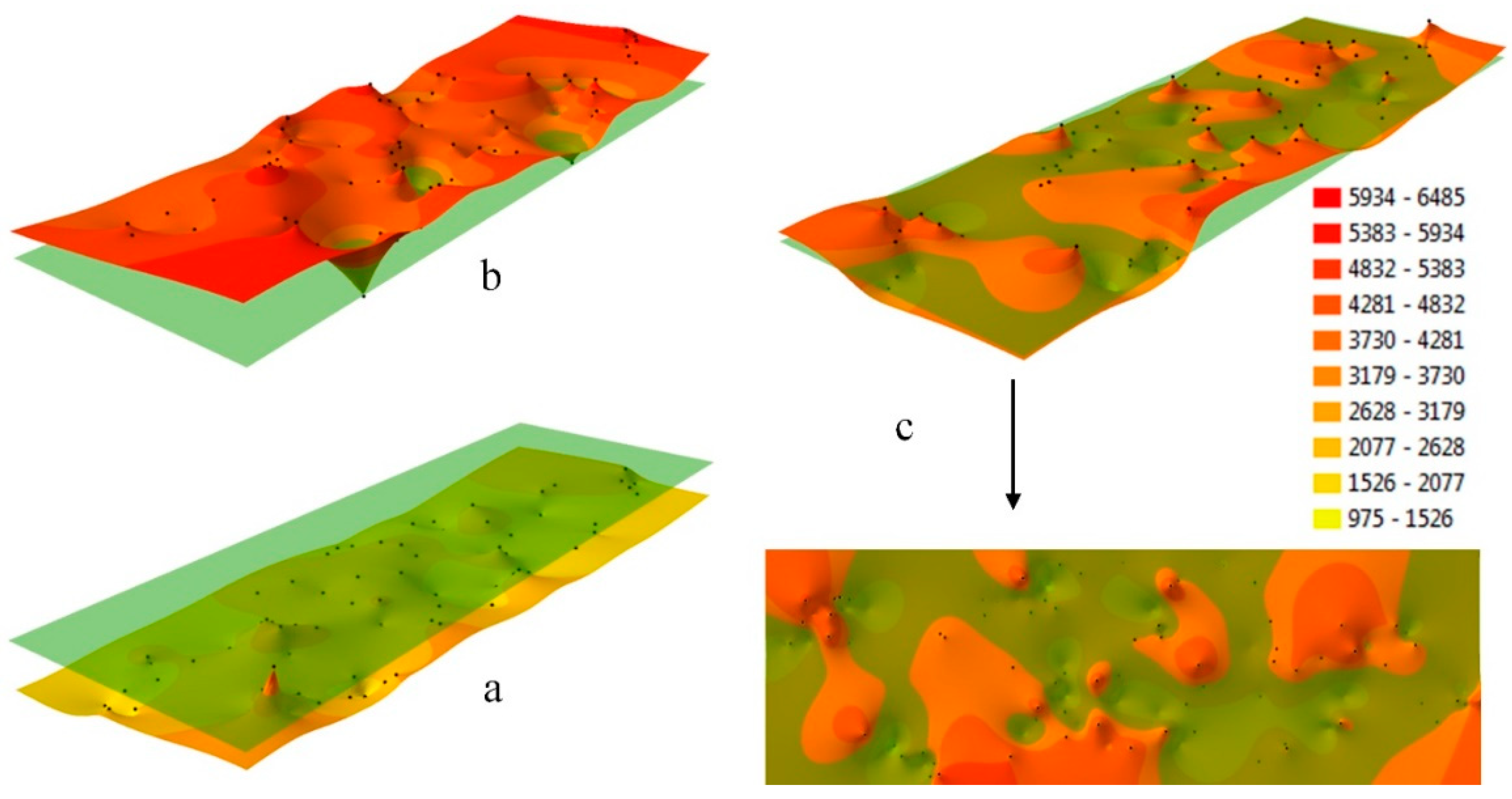
A surface model generated with a GRID structure is presented in Figure 3. A network of nodes with 0.0005° resolution was created in the analyzed area in the adopted coordinate system (WGS 84 Web Mercator), which supported the generation of 1386 model points (Figure 3a). Measurement points (Figure 1a) were used to calculate the interpolated value in each node with the use of the K algorithm. The resulting GRID structure was used to generate the interpolated surface, which is presented in Figure 3b,c.

3.2. Selection of GRID Structure Resolution

The selection of the structural parameters of the network of squares describing the analyzed model of interpolation space is an equally important stage of the analysis. The parameters of a GRID structure are selected in view of its resolution which determines the size of the square base in the network which, in turn, defines the size of the base field where data from a given epoch can be analyzed. The location of nodes can be described freely, which supports smooth adjustment of network resolution to specific precision guidelines. Two resolutions of a GRID structure generated based on the same dataset (Figure 1a) are presented in Figure 4. In the first case, the side of the square base was determined at 0.0005°, which supported the generation of 1386 nodes in the analyzed object. In an enlarged fragment of the interpolated surface, the location of network nodes is presented relative to the group of five measurement points used in the example.

Network nodes do not overlap measurement points due to the large size of the square base. The interpolated values in those nodes differ from the measured values, which produces a worse fit between the generated interpolated surface and the surface formed by measurement points. The size of the square bases forming the network can be determined by the precision of the horizontal coordinates of the analyzed measurement points. In the presented example, the estimation error of horizontal coordinates of every measurement point (geometric center of each building) was set at 0.0001°.

The resulting increase in GRID resolution supported the generation of 32,240 nodes in the analyzed object (Figure 4b). In an enlarged fragment of the interpolated surface, the location of nodes is presented relative to the same group of five measurement points.

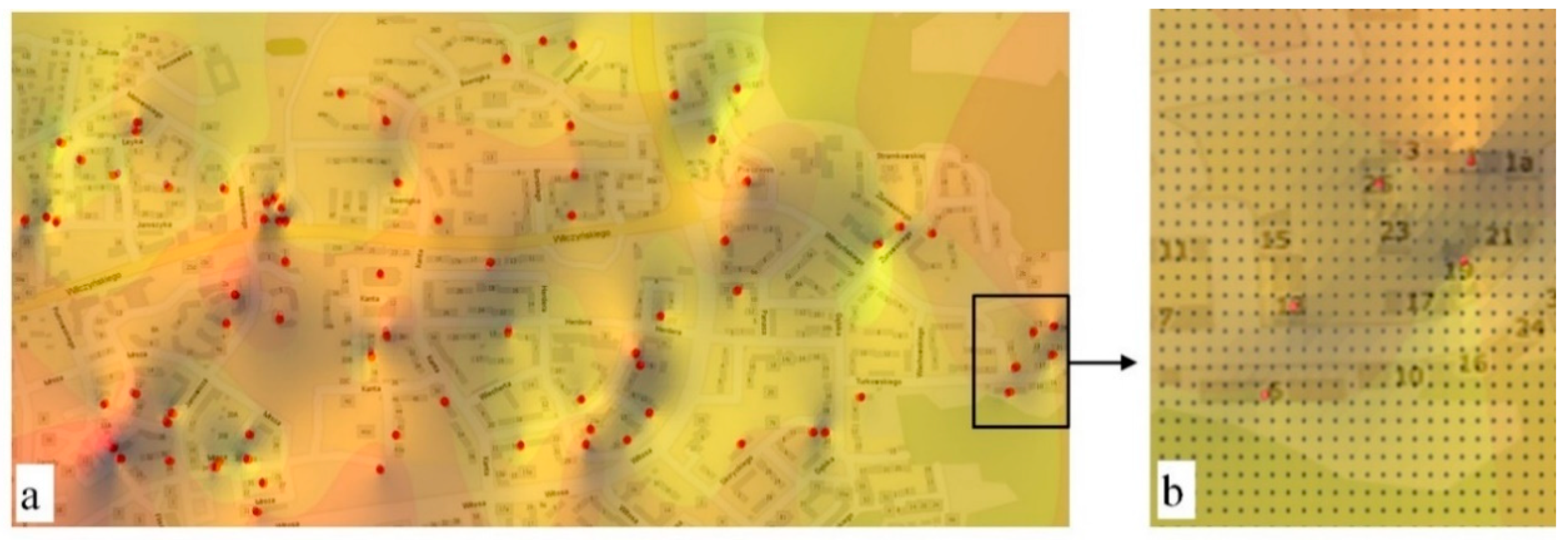
Higher-resolution supported the localization of nodes near measurement points within the margin of error for estimating the horizontal coordinates of every measured point. When the size of a base field is decreased, data can be analyzed with greater precision, and all lines separating class intervals can be interpolated more smoothly. The selected interpolation algorithm was used to assign near-market values to groups of interpolation nodes located closest to the measurement points. Surfaces created based on the nodes of the GRID network with 0.0001° resolution can be used to determine property value zones localized in the analyzed object with given precision (Figure 5a). When the size of a base field is adapted to the size of the measured objects (buildings), selected apartments can be localized in interpolated zones of property values (Figure 5b). The influence of the prices of neighboring properties on the value of the analyzed object can be examined.

3.3. Analysis of Numerical Models

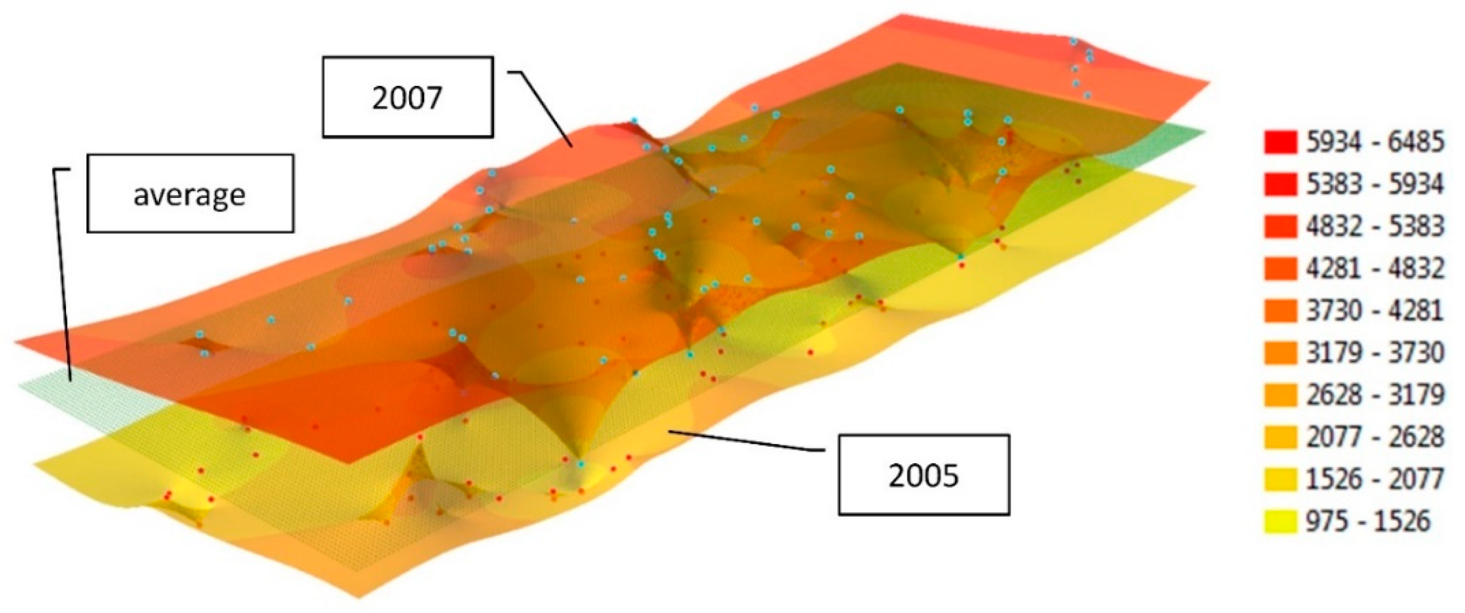
Irregularly distributed measurement points can be replaced with a regular node network to compare interpolation models across epochs. The generated surfaces can be used to compare measurements performed in different periods of time with different distribution and resolution of the measured objects. Measurement data can also be replaced with a mathematically defined node network to compare the values generated in successive epochs in each node with the average price in a given period, represented by a horizontal plane. The location of three interpolated surfaces (generated based on GRID structures with 0.0001° resolution) relative to the average value for the entire measurement period is presented in Figure 6. The overall average, calculated by assigning weights to the number of apartments traded in successive years, was determined at PLN 3780.80/m². In the first case (Figure 6a), the interpolated surface was generated based on data for 2005. Excluding one case, the interpolation model is located below the plane representing the average price. The presented epoch (2005) was characterized by the lowest real estate prices.

In the second case (Figure 6b), an interpolation model was generated for 2007 values, and the horizontal coordinates of nodes were identical to those in the first example. In the presented model, most interpolation nodes are situated above the average for the analyzed period. This epoch (2007) was characterized by the highest real estate prices. The third example (Figure 6c) represents an epoch (2014) where prices approximated the average. In this case, the horizontal coordinates of nodes were also identical to those noted in the previous examples.

The surface models generated by a GRID structure based on extreme values from selected epochs can be used to analyze the range of fluctuations in property prices in the examined period. In Figure 7, models generated for epochs with extreme values are compared against one another and against the average for the analyzed period. 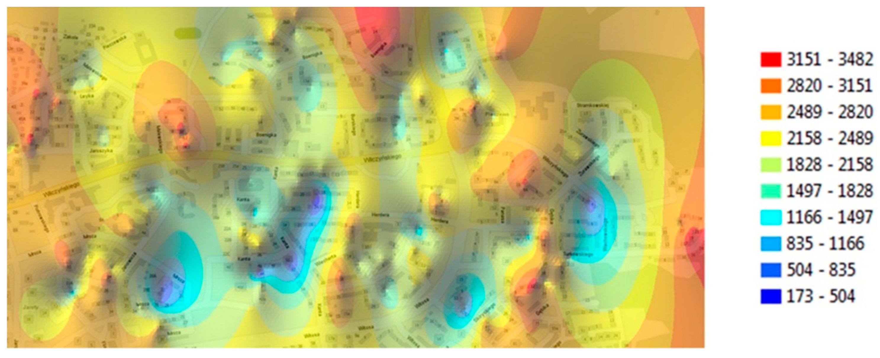An analysis can be performed in the same nodes despite different locations of measurement points in each epoch (Figure 7). The generated nodes are uniformly distributed despite differences in the local density of measurement points. Local extrema, as well as areas characterized by similar property prices, can be determined in the compared epochs. Nodes with identical locations can also be used to determine differences in values between epochs and to present them in a differential diagram. A differential diagram generated based on differences in property prices in 2005 and 2007 is presented in Figure 8. The diagram was adapted to the examined object with the use of all measurement points in both epochs. The calculated values were assigned to 10 equal class intervals, which supported the identification of differential price zones for both extreme and middle values. Analyses of the type are performed to determine areas with the highest and lowest price fluctuations in a given period as well as areas where property prices remained stable.

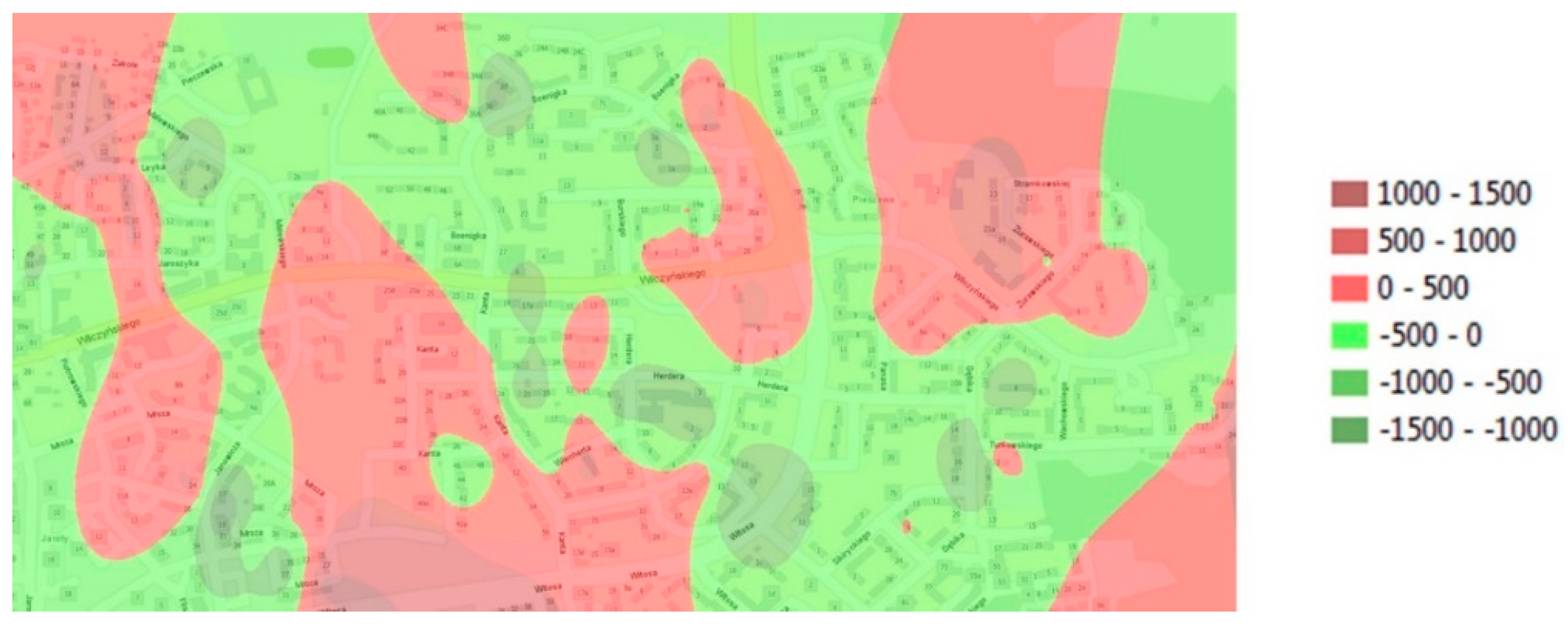
Differential diagrams generated for every epoch relative to the average for the entire period of analysis can also be used to visualize areas characterized by different property prices. Such diagrams are applied when local extrema disrupt the values of the calculated indicators (Equations (1)–(4)). The diagrams are generated based on differences in the values of nodes and the arithmetic mean of prices for the entire period of analysis. A differential diagram for 2014 is presented in Figure 9. The classification intervals of differential values support the identification of areas where property prices are above or below the average for all epochs. In the presented example, the differences are positive (above average—marked in red) and negative (below average—marked in green).

3.4. Interpretation of Statistical Indicators

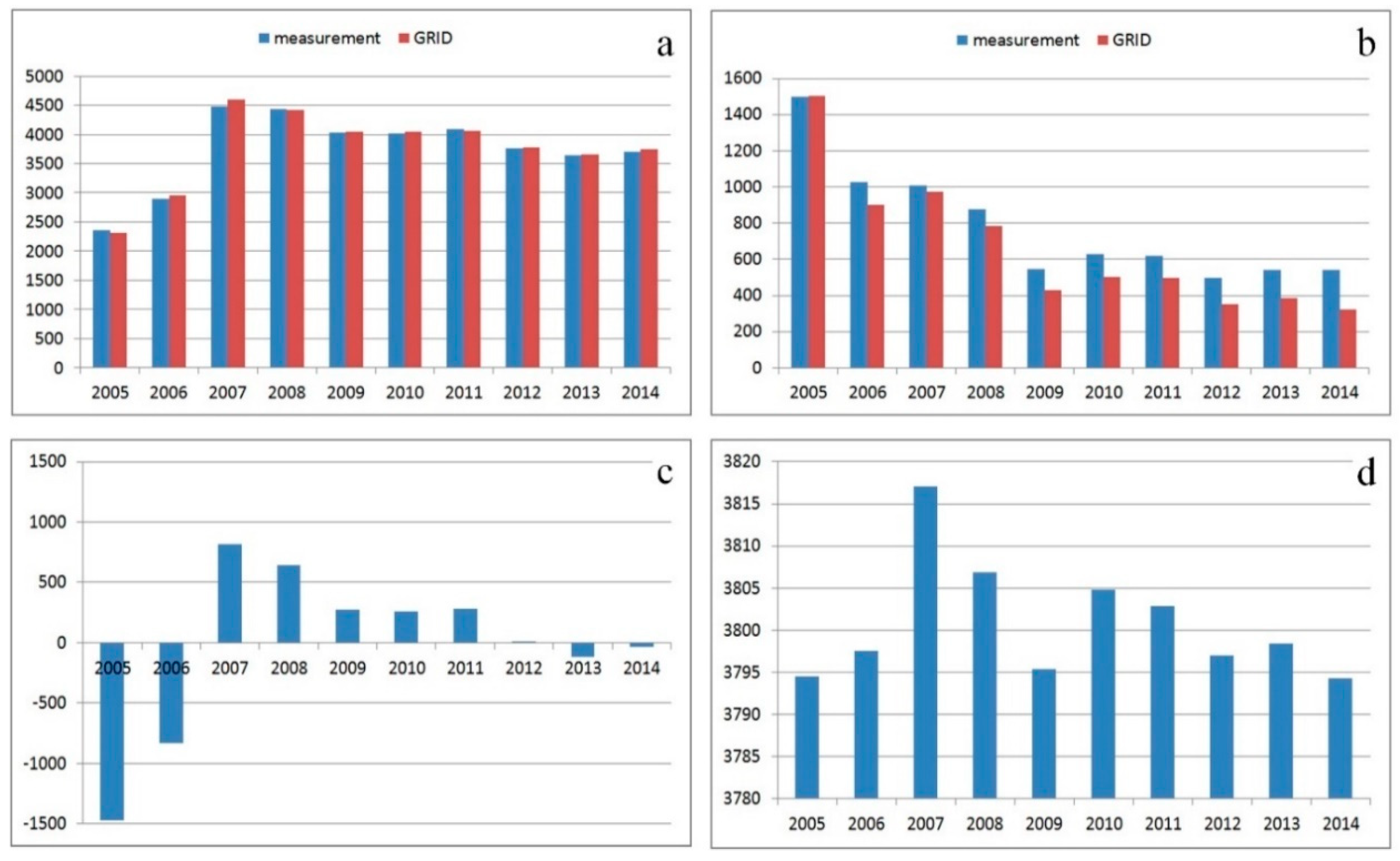
Equations (1)–(4) were applied to calculate the indicators in every epoch. Statistical indicators for successive epochs are presented in Figure 10. In Figure 10a,b, statistical indicators determined for GRID nodes are accompanied by the same indicators calculated for measurement points only. This approach supports an evaluation of the fit between the GRID interpolated surface and the TIN surface. The variations in the values of the calculated indicators result from differences in the number of data. The number of measurement points ranged from 80 to 135 in different epochs, and the number of interpolation nodes for 0.0001° resolution was determined at 32,340, and it remained stable across epochs. Interpolation leads to minor surface generalization. Despite minor differences in the presented values, the correlations between successive epochs are identical, and they can be compared with the use of a GRID structure.

The average value of measurements computed by the conventional method and the absolute value of the average in GRID nodes calculated with Equation (2) are compared in Figure 10a. The two indicators demonstrate that the average property price was the lowest in 2005 and the highest in 2007. The average price was stabilized at PLN 4100/m² in 2009–2011, and it decreased to a stable level of PLN 3700/m² in 2012–2014.

The values of RMSE in Equation (4) calculated based on measured data and GRID nodes are compared in Figure 10b. The fit to average surface values generated for successive epochs is presented and compared in the diagrams. The measurements conducted in 2005 were characterized by the least satisfactory fit to the plane generated based on the average value for the investigated period (Figure 6a). Most values are localized on the side of the plane representing the average value (below average), and excluding one case, none of the values compensate for the resulting RMSE. In 2007 (Figure 6b), most values were also localized on only one side of the plane representing the average price (above average), but in this case, all values were closer to the average. In 2009–2014, property prices were similar, and they were characterized by similar relationships with the average price (a similar number of prices above and below the average for that period). The best fit between the surface generated by the average price and the interpolated surface was observed in 2012 and 2014 (Figure 6c).

The average differences in the values assigned to GRID nodes are presented in Figure 10c. The differences were calculated between the value interpolated in a given epoch and the value determined by the average for the entire period. The diagrams indicate the years in which most real estate was valued below the average (negative values) and above the average (positive value). Most objects were priced below the average in 2005–2006 and above the average in 2007–2011. Property prices were closest to the average in 2012 and 2014, which is shown in Figure 10b (lowest RMSE). The standard deviation of node values in a GRID structure, calculated with Equation (3), is presented in Figure 10d. The diagram contains information about differences in property prices (attribute variations within a set) in every epoch as well as values that diverge most from the average. The greatest variation within a dataset was noted in 2007 (Figure 6a). This epoch was characterized by the most significant price fluctuations. The data in Figure 6a suggest that those variations occurred locally. The smallest fluctuations in property prices were noted in 2005, 2009 and 2014. The interpolated surfaces generated for those epochs most closely resembled a plane (Figure 6a,c). The greatest deviation from the average price was noted in 2007 and the smallest deviation was observed in 2014 (Figure 10d).

4. Discussion

Due to the advantages and the considerable potential of a GRID structure, the presented analytical method offers a viable alternative to the interpolation methods that are presently deployed in real estate market analyses [12,13,14,15,16,17,49]. The choice of the most appropriate interpolation algorithm and optimal GRID resolution supports the generation of continuous interpolated surfaces while maintaining the values of measurement points. Uniform distribution of nodes in a GRID structure preserves the continuity of the model and supplements missing fragments in the modeled surface. The structure of points creating a surface model should be organized to speed up analysis and improve the effectiveness of data modeling and archiving. When a GRID structure is used, the resolution of network nodes forming the surface model can also be increased. When the number of points (nodes) is increased, the surface can be described with greater resolution, and analyses can be performed in areas without measurement points.

A GRID structure with higher resolution supported the localization of nodes near measurement points within the margin of error for estimating the horizontal coordinates of every measured point. When the size of a base field is decreased, data can be analyzed with greater precision, and all lines separating class intervals can be interpolated more smoothly. The selected interpolation algorithm was used to assign near-market values to groups of interpolation nodes located closest to the measurement points. In a TIN structure with a small number of measurement points, the generated surface models have low resolution and quality [50]. The above is not always the case in a GRID structure which supports the generation of networks where the resolution of nodes exceeds the density of measurement points alone. Resolution can be improved through the use of base squares with the required size and by performing the interpolation process based on the appropriately localized measurement points or nodes that were previously generated in a given area. Higher node density supports more detailed descriptions of the model in selected locations and more accurate analyses at any given point.

Changes in the model over time can also be assessed when the location of GRID nodes is strictly mathematically determined. When this structure is used, comparative analyses can be conducted in the same points in space in different measurement epochs (years). The above solution can be deployed to forecast the behavior of the modeled space over time.

The proposed method also supports the localization of and compensation for measurement extrema. In the model developed with a GRID structure, interpolation algorithms facilitate compensation for extreme values at a given level of accuracy. The resulting model approximates the shape of space in a manner that facilitates shape analysis. The above compensates for the irregularities of the TIN model [51,52,53,54,55], while maintaining the shape of the examined surface, which facilitates the relevant analyses. A GRID structure can be thus used to analyze highly complex data in real estate markets characterized by low transparency and low availability of reliable data.

Above all, the precise structural description of a surface model considerably speeds up data processing and modeling. The above accelerates database analyses and the search for the desired information.

The universal approach to processing GRID structures in the proposed methodology facilitates analyses of different measurements and the formulation of functional assumptions in various fields of research. Considerable amounts of data describing the attributes of the evaluated objects are recorded in a similar manner (object location and object attributes); therefore, the developed methodology can be applied in comprehensive analyses of similar cases.

The absence of continuous data on real estate prices in a given location poses a significant problem in analyses of the real estate market which plays a key role in the functioning of the entire real estate industry. The proposed solution increases the accuracy of multidimensional spatiotemporal analyses of the real estate market based on dispersed transaction data. As demonstrated in the study, GRID models support analyses and predictions of changes over time, complex comparisons of real estate prices in different epochs (years) and effective archiving of resources both for individual GRID nodes and the entire analyzed space. Data relating to market transactions can also be converted into a mathematically defined grid of nodes for analyzing and predicting values (real estate prices and values) at any point in time with the required accuracy. Such analyses can be performed in base fields of any size by generating GRID structures with a freely regulated resolution. This approach to archiving and analyzing real estate market data supports dynamic data processing. The described tool increases the accuracy of real estate market analyses and supports dynamic data processing, and it can be highly useful for market participants, including buyers, tenants and developers. The above factors play a particularly important role in analyses of transactions conducted on a large scale (cities, regions or even countries) that involve extensive sets of dispersed data concerning transactions, prices and longtime intervals. The real estate industry is characterized by high dynamics, variability and unpredictability, and models based on GRID structures can significantly facilitate real estate analyses and monitoring.

5. Conclusions

Methods that rely on GRID structures are a valuable tool for urban real estate market analyses. The spatial distribution of values constitutes the main source of information for market participants. The existing interpolation methods are characterized by a high degree of generalization and, consequently, limited accuracy. This problem largely detracts from the effectiveness of the generated models. The proposed interpolation method, developed based on a GRID structure, is characterized by much higher precision and effectiveness, which supports more accurate and varied analyses of property prices in space and time. A GRID interpolated surface can be used to analyze changes in any point of the investigated area and to perform comparisons with surfaces generated in other epochs. When the points on a GRID surface are distributed in a uniform fashion (Figure 3c), changes in value can be evaluated more accurately than when a TIN surface (Figure 1c) is used for the same object. In TIN structures, the density, number and location of measurement points differ across epochs and cannot be directly compared. In GRID structures, data can be compared because the size of the base field is identical for all epochs. Any two fragments (represented by nodes) of interpolated surfaces can be compared despite differences in the number, location and local density of measurement points. The comparison can be performed for any time intervals. The values assigned to nodes in the analyzed area can also be included in selected layers of data in SIS. This approach supports comparisons with datasets that are stored in other SIS data layers.

The presented solution supports the generation of any space that approximates real space, and it can be used to control the accuracy of the consecutive stages of the procedure and to select the appropriate processing sequences during the entire process. The application of the GRID structure at various processing stages facilitates the organization of data and the application of similar control mechanisms to compare the accuracy of the consecutive stages of the analytical process. As a result, the processing stages, including the analysis of the measured data, generation of a GRID structure and its use in various practical applications, can be optimized. The proposed methodology supports highly dynamic data processing and considerable automation in consecutive stages of the process. The coherence of consecutive processing stages ensures that a full set of data will be examined comprehensively in statistical analyses. The accuracy of the generated models is controlled; therefore, the most effective solutions to the analyzed problems can be formulated in every stage of the process.

References

- Goodman, A.C.; Thibodeau, T.G. Housing market segmentation. J. Hous. Econ. 1998, 7, 121–143. [Google Scholar] [CrossRef]
- Jones, C.; Leishman, C.; Watkins, C. Structural change in a local urban housing market. Environ. Plan. 2003, 35, 1315–1326. [Google Scholar] [CrossRef]
- Bourassa, S.C.; Cantoni, E.; Hoesli, M. Spatial dependence, housing submarkets, and house price prediction. J. Real Estate Financ. Econ. 2007, 35, 143–160. [Google Scholar] [CrossRef] [Green Version]
- Case, B.; Clapp, J.; Dubin, R.; Rodriguez, M. Modeling spatial and temporal house price patterns: A comparison of four models. J. Real Estate Financ. Econ. 2004, 29, 167–191. [Google Scholar] [CrossRef]
- Chiang, Y.H.; Peng, T.C.; Chang, C.O. The nonlinear effect of convenience stores on residential property prices: A case study of Taipei, Taiwan. Habitat Int. 2015, 46, 82–90. [Google Scholar] [CrossRef]
- Dubin, R.; Pace, K.; Thibodeau, T. Spatial autoregression techniques for real estate data. J. Real Estate Lit. 1999, 7, 79–95. [Google Scholar] [CrossRef]
- Leishman, C.; Costello, G.; Rowley, S.; Watkins, C. The predictive performance of multilevel models of housing sub-markets: A comparative analysis. Urban Stud. 2013, 50, 1201–1220. [Google Scholar] [CrossRef] [Green Version]
- Nygaard, C.; Meen, G. The Distribution of London Residential Property Prices and the Role of Spatial Lock-in. Urban Stud. 2013, 50, 2535–2552. [Google Scholar] [CrossRef]
- Pace, R.K.; Barry, R.; Gilley, O.W.; Sirmans, C.F. A method for spatial–temporal forecasting with an application to real estate prices. Int. J. Forecast. 2000, 16, 229–246. [Google Scholar] [CrossRef]
- Torre, A.; Pham, V.H.; Simon, A. The ex-ante impact of conflict over infrastructure settings on residential property values: The case of Paris’s suburban zones. Urban Stud. 2014, 52, 2404–2424. [Google Scholar] [CrossRef]
- Zhou, P.; Liu, Y.; Chen, Y.; Zeng, C.; Wang, Z. Prediction of the spatial distribution of high-rise residential buildings by the use of a geographic field based autologistic regression model. J. Hous. Built Environ. 2014, 30, 487–508. [Google Scholar] [CrossRef]
- Kunz, M.; Helbich, M. Geostatistical mapping of real estate prices: An empirical comparison of kriging and cokriging. Int. J. Geogr. Inf. Sci. 2014, 28, 1904–1921. [Google Scholar] [CrossRef]
- Li, L.; Revesz, P. Interpolation Methods for Spatio-temporal Geographic Data. Comput. Environ. Urban Syst. 2004, 28, 201–227. [Google Scholar] [CrossRef]
- McCluskey, W.J.; Deddis, W.G.; Lamont, I.G.; Borst, R.A. The application of surface generated interpolation mels for the prediction of residential property values. J. Prop. Invest. Financ. 2000, 18, 162–176. [Google Scholar] [CrossRef] [Green Version]
- Montero, J.; Larraz, B. Interpolation methods for geographical data: Housing and commercial establishment markets. J. Real Estate Res. 2011, 33, 233–244. [Google Scholar]
- Pagourtzi, E.; Assimakopoulos, V.; Hatzichristos, T.; French, N. Real estate appraisal: A review of valuation methods. J. Prop. Invest. Financ. 2003, 21, 383–401. [Google Scholar] [CrossRef] [Green Version]
- Szczepańska, A.; Senetra, A.; Wasilewicz-Pszczółkowska, M. The effect of road traffic noise on the prices of residential property—The example of a European city. Transp. Res. Part D 2015, 36, 167–177. [Google Scholar] [CrossRef]
- Chou, Y.H. Exploring Spatial Analysis in Geographic Information Systems; OnWord Press: Santa Fe, NM, USA, 1997. [Google Scholar]
- Basu, S.; Thibodeau, T.G. Analysis of spatial autocorrelation in house prices. J. Real Estate Financ. Econ. 1998, 17, 61–85. [Google Scholar] [CrossRef]
- Osland, L. An Application of Spatial Econometrics in Relation to Hedonic House Price Modeling. J. Real Estate Res. 2010, 32, 289–320. [Google Scholar]
- Tu, Y.; Sun, H.; Yu, S.M. Spatial autocorrelations and urban housing market segmentation. J. Real Estate Financ. Econ. 2007, 34, 385–406. [Google Scholar] [CrossRef]
- Del Giudice, V.; De Paola, P.; Torrieri, F.; Nijkamp, P.J.; Shapira, A. Real Estate Investment Choices and Decision Support Systems. Sustainability 2019, 11, 3110. [Google Scholar] [CrossRef] [Green Version]
- Goodchild, M.F. Geographic information systems and science: Today and tomorrow. Ann. GIS 2009, 15, 3–9. [Google Scholar] [CrossRef] [Green Version]
- Longley, P.A.; Goodchild, M.F.; Maguire, D.J.; Rhind, D.W. Geographical Information Systems and Sience, 3rd ed.; Wiley: Hoboken, NJ, USA, 2011. [Google Scholar]
- Andrienko, N.; Andrienko, G. Exploratory Analysis of Spatial and Temporal Data A Systematic Approach; Springer: Berlin, Germany, 2006. [Google Scholar]
- Johannesson, G.; Cressie, N.; Huang, H.C. Dynamic multiresolution spatial models. Environ. Ecol. Stat. 2007, 14, 5–25. [Google Scholar] [CrossRef]
- Hastie, T.; Tibshirani, R.; Friedman, J. The Elements of Statistical Learning. Data Mining, Inference, and Prediction; Springer Publishing Company: New York, NY, USA, 2009. [Google Scholar]
- Huang, Y.; Pei, J.; Xiong, H. Mining colocation patterns with rare events from spatial data sets. Geoinformatica 2006, 10, 239–260. [Google Scholar] [CrossRef] [Green Version]
- Miller, H.; Han, J. Geographic data mining and knowledge discovery: An overview. In Geographic Data Mining and Knowledge Discovery; Miller, H., Han, J., Eds.; CRC Press: Boca Raton, FL, USA, 2009; pp. 1–26. [Google Scholar]
- Soares, T. Deductive Database. Implementatio Parallelism and Applications; ICLP Springer: Berlin/Heidelberg, Germany, 2006. [Google Scholar]
- Harris, R.; Sleight, P.; Webber, R. Geodemographies, GIS and Neighbourhood Targeting; Wiley: Chichester, UK, 2005. [Google Scholar]
- Dean, J.; Ghemawat, S. MapReduce: Simplified data processing on large clusters. Commun. ACM 2008, 51, 107–113. [Google Scholar] [CrossRef]
- Masser, L. Spatial Data Lnfrastructure: An Introduction; ESRI Press: Redlands, CA, USA, 2005. [Google Scholar]
- Fischer, M.M. Spatial Analysis and GeoComputation; Springer: Berlin, Germany, 2006. [Google Scholar]
- Proulx, M.J.; Bédard, Y. Fundamental Characteristics of Spatial OLAP Technologies as Selection Criteria; Location Intelligence: Santa Clara, CA, USA, 2008. [Google Scholar]
- Chen, C.F.; Li, Y.Y.; Dai, H.L. An application of Coons patch to generate grid- based digital elevation models. Int. J. Appl. Earth Obs. Geoinf. 2001, 13, 830–837. [Google Scholar] [CrossRef]
- Gosciewski, D. Ustalenie wielkości siatki bazowej GRID w zależności od ukształtowania terenu. Zesz. Nauk. Politech. Rzesz. Bud. Inżynieria Środowiska 2012, 59, 121–133. [Google Scholar]
- Raaflaub, L.D.; Collins, M.J. The effect of error in gridded digital elevation models on the estimation of topographic parameters. Environ. Model. Softw. 2006, 21, 710–732. [Google Scholar] [CrossRef]
- Jóźwiak, J.; Podgórski, J. Statystyka od Podstaw; PWE: Warsaw, Poland, 2000. [Google Scholar]
- Paradysz, J. Statystyka; Wydawnictwo AE: Poznań, Poland, 2005. [Google Scholar]
- Suchecki, B. Ekonometria Przestrzenna; Wydawnictwo, C.H., Ed.; Beck: Warsaw, Poland, 2010. [Google Scholar]
- Gosciewski, D. The effect of the distribution of measurement points around the node on the accuracy of interpolation of the digital terrain model. J. Geogr. Syst. 2013, 15, 513–535. [Google Scholar] [CrossRef] [Green Version]
- Tay, L.T.; Sagar, B.S.D.; Chuah, H.T. Analysis of geophysical networks derived from multiscale digital elevation models: A morphological approach. IEEE Geosci. Remote Sens. Lett. 2005, 2, 399–403. [Google Scholar] [CrossRef]
- Wechsler, S.P. Perceptions of digital elevation model uncertainty by DEM users. URISA J. 2003, 15, 57–64. [Google Scholar]
- Deng, X.S.; Tang, Z.A. Moving surface spline interpolation based on Green’s function. Math. Geosci. 2011, 43, 663–680. [Google Scholar] [CrossRef]
- Erdogan, S. A comparison of interpolation methods for producing digital elevation models at the field scale. Earth Surf. Process. Landf. 2009, 34, 366–376. [Google Scholar] [CrossRef]
- Gosciewski, D. Reduction of deformations of the digital terrain model by merging interpolation algorithms. Comput. Geosci. 2014, 64, 61–71. [Google Scholar] [CrossRef]
- Larsson, E.; Fornberg, B. Theoretical and computational aspects of multivariate interpolation with increasing flat basis functions. Comput. Math. Appl. 2005, 49, 103–130. [Google Scholar] [CrossRef] [Green Version]
- Hu, S.; Cheng, Q.; Wang, L.; Xie, S. Multifractal characterization of urban residential land price in space and time. Appl. Geogr. 2012, 34, 161–170. [Google Scholar] [CrossRef]
- Webster, R.; Oliver, M. Geostatistics for Environmental Scientists Statistics in Practice; Wiley: Chichester, UK, 2001. [Google Scholar]
- Calka, B. Estimating Residential Property Values on the Basis of Clustering and Geostatistics. Geosciences 2019, 9, 143. [Google Scholar] [CrossRef] [Green Version]
- Cellmer, R. The possibilities and limitations of geostatistical methods in real estate market analyses. Real Estate Manag. Valuat. 2014, 22, 54–62. [Google Scholar] [CrossRef] [Green Version]
- Chica-Olmo, J. Prediction of housing location price by a multivariate spatial method: Cokriging. J. Real Estate Res. 2007, 29, 91–114. [Google Scholar]
- Zhang, Z.; Lu, X.; Zhou, M.; Song, Y.; Luo, X.; Kuang, B. Complex spatial morphology of urban housing price based on digital elevation model: A case study of Wuhan city, China. Sustainability 2019, 11, 348. [Google Scholar] [CrossRef] [Green Version]
- Zhang, Z.; Tan, S.; Tang, W. A GIS-based spatial analysis of housing price and road density in proximity to urban lakes in Wuhan City, China. Chin. Geogr. Sci. 2015, 25, 775–790. [Google Scholar] [CrossRef] [Green Version]
© 2020 by the authors. Licensee MDPI, Basel, Switzerland. This article is an open access article distributed under the terms and conditions of the Creative Commons Attribution (CC BY) license (http://creativecommons.org/licenses/by/4.0/).