Examining Land Use/Land Cover Change and the Summertime Surface Urban Heat Island Effect in Fast-Growing Greater Hefei, China: Implications for Sustainable Land Development


Abstract
:
1. Introduction
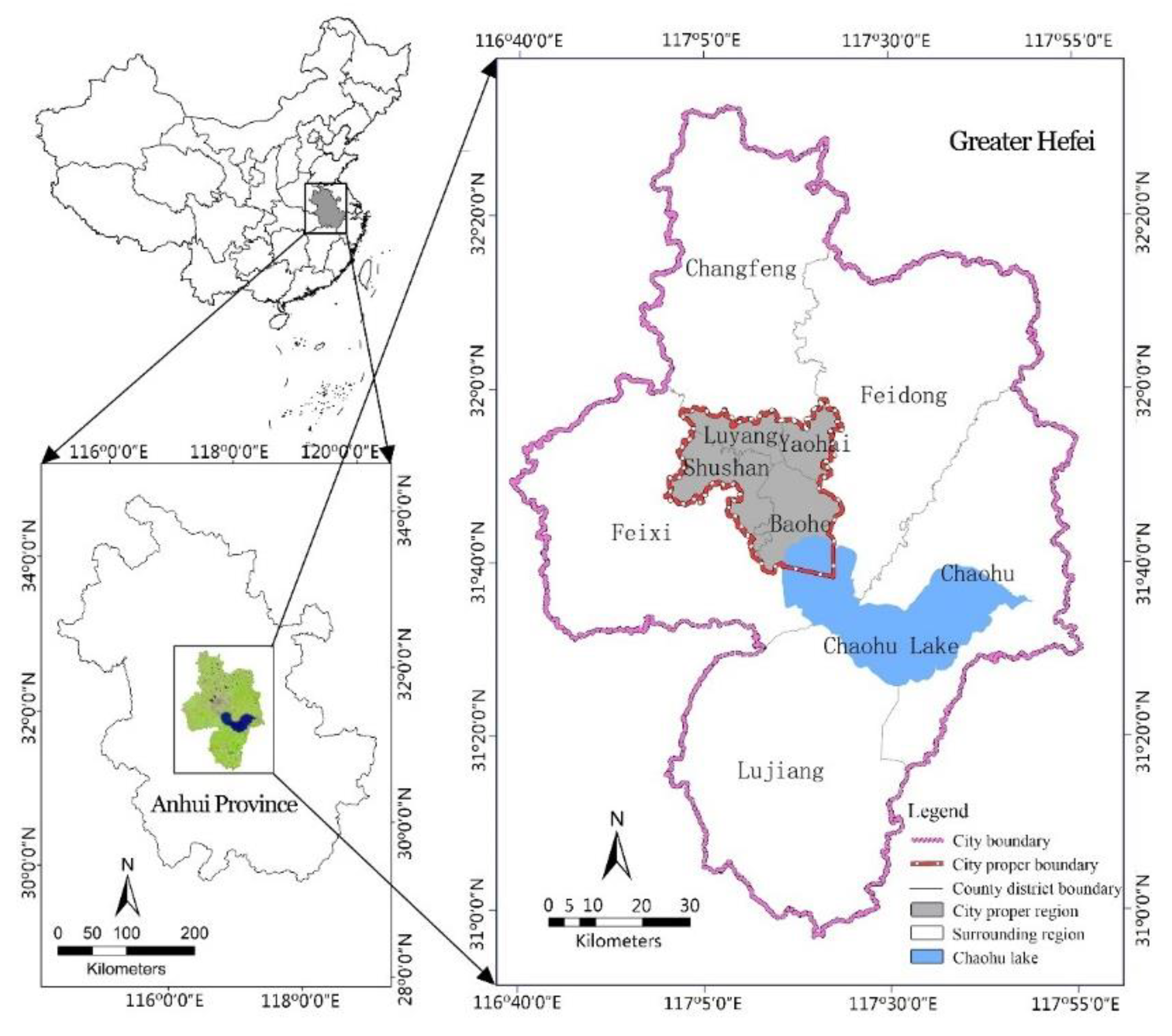
2. Study Region
3. Materials and Methods
3.1. Data Sources
3.2. Methods
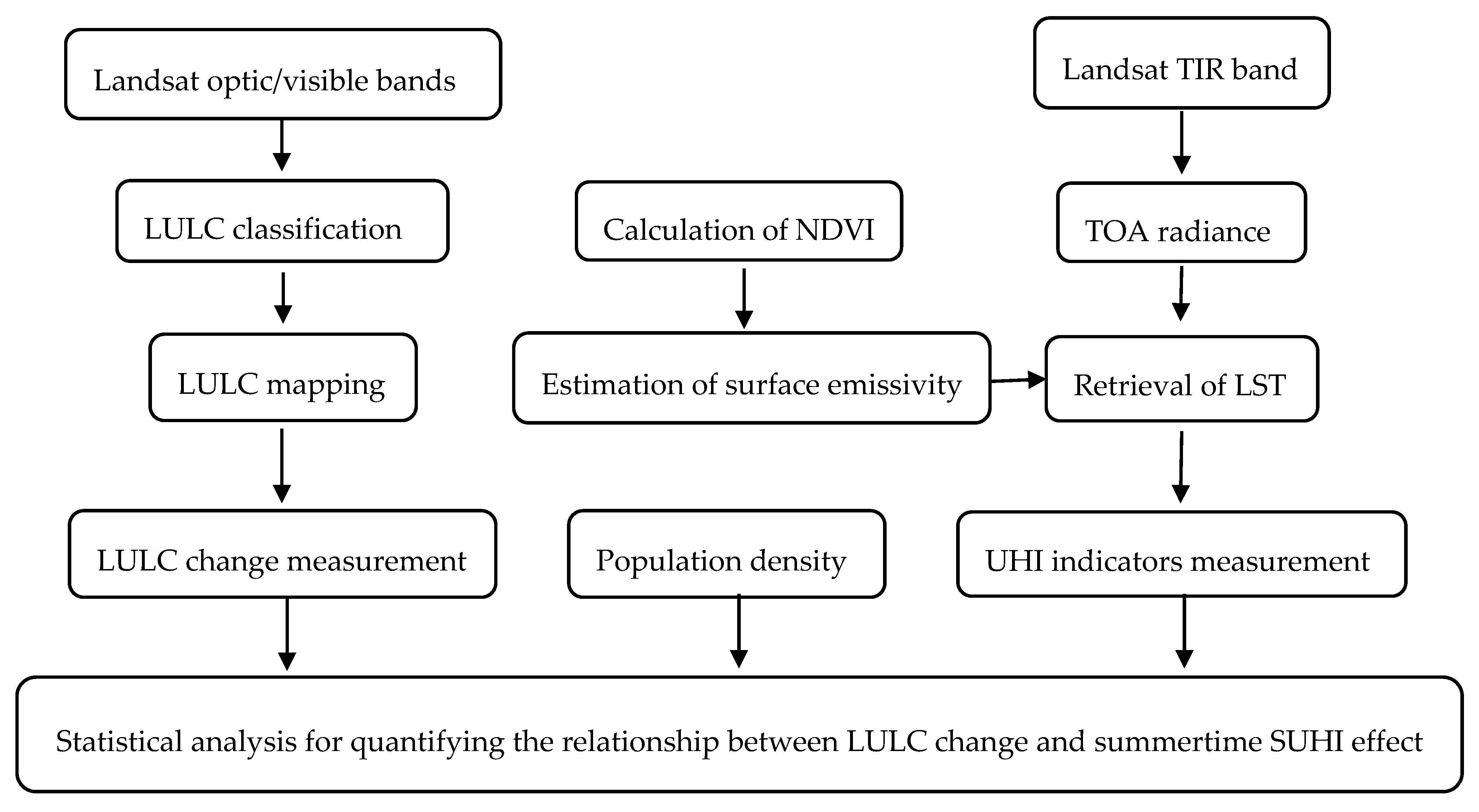
3.2.1. Processing of Satellite Imagery
3.2.2. LULC Change Measurement
3.2.3. Retrieval of LST
3.2.4. Measuring Summertime UHI Effect Indicators
3.2.5. Statistical Analysis
4. Results
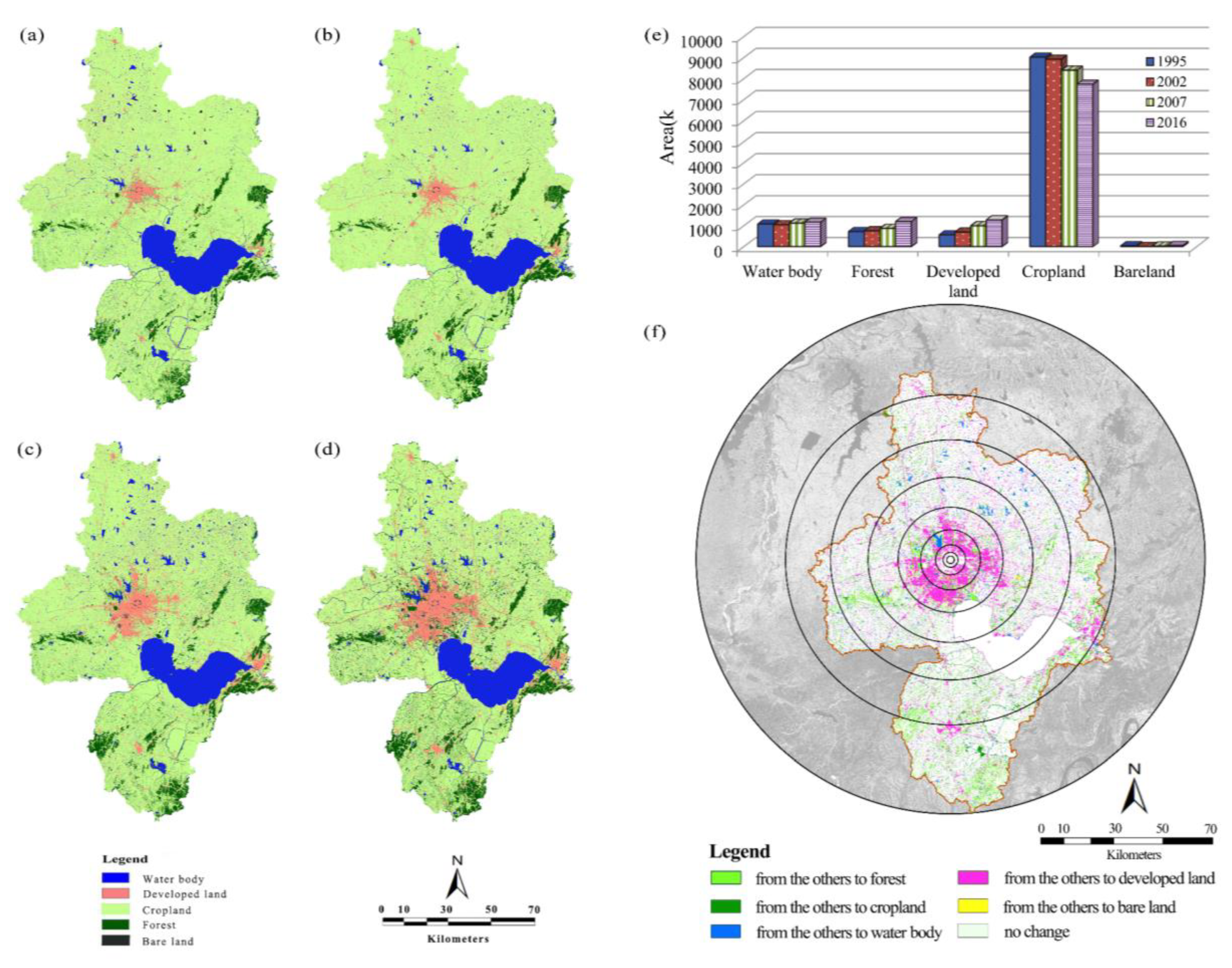
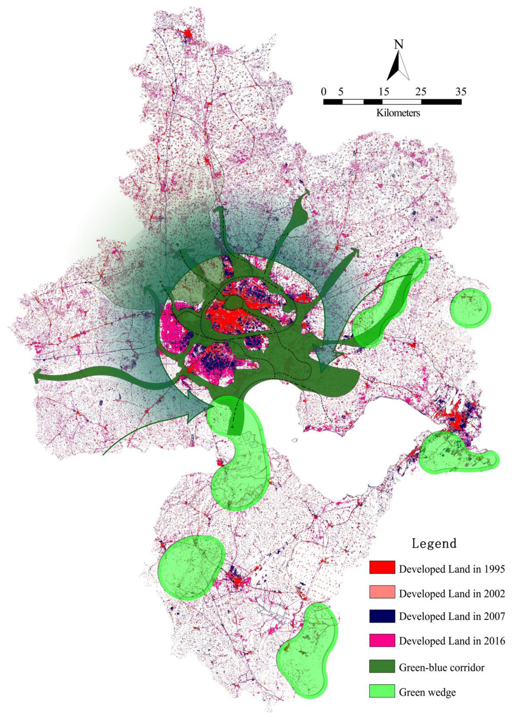
4.1. Synoptic Analysis of LULC Change at the Regional Level
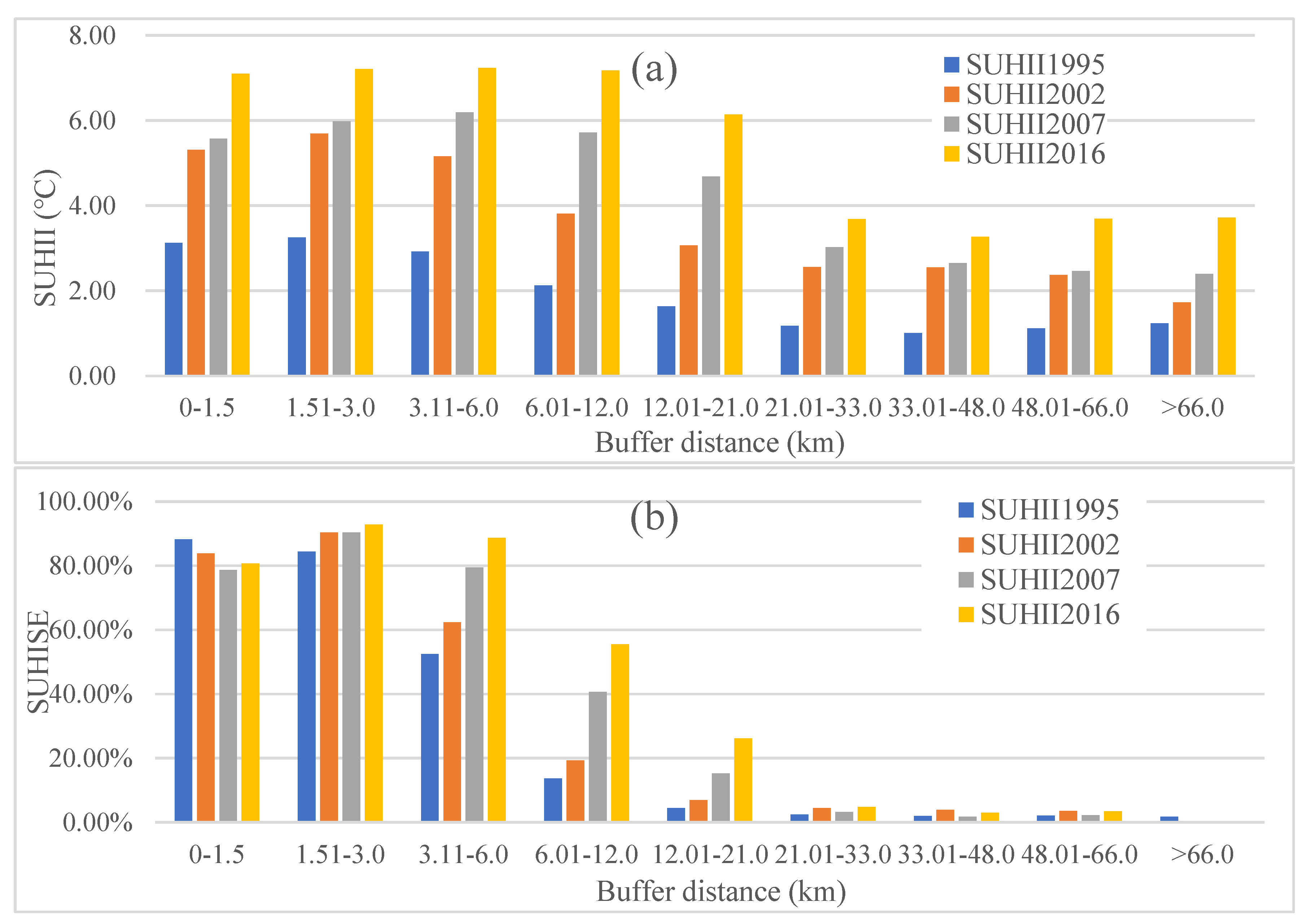
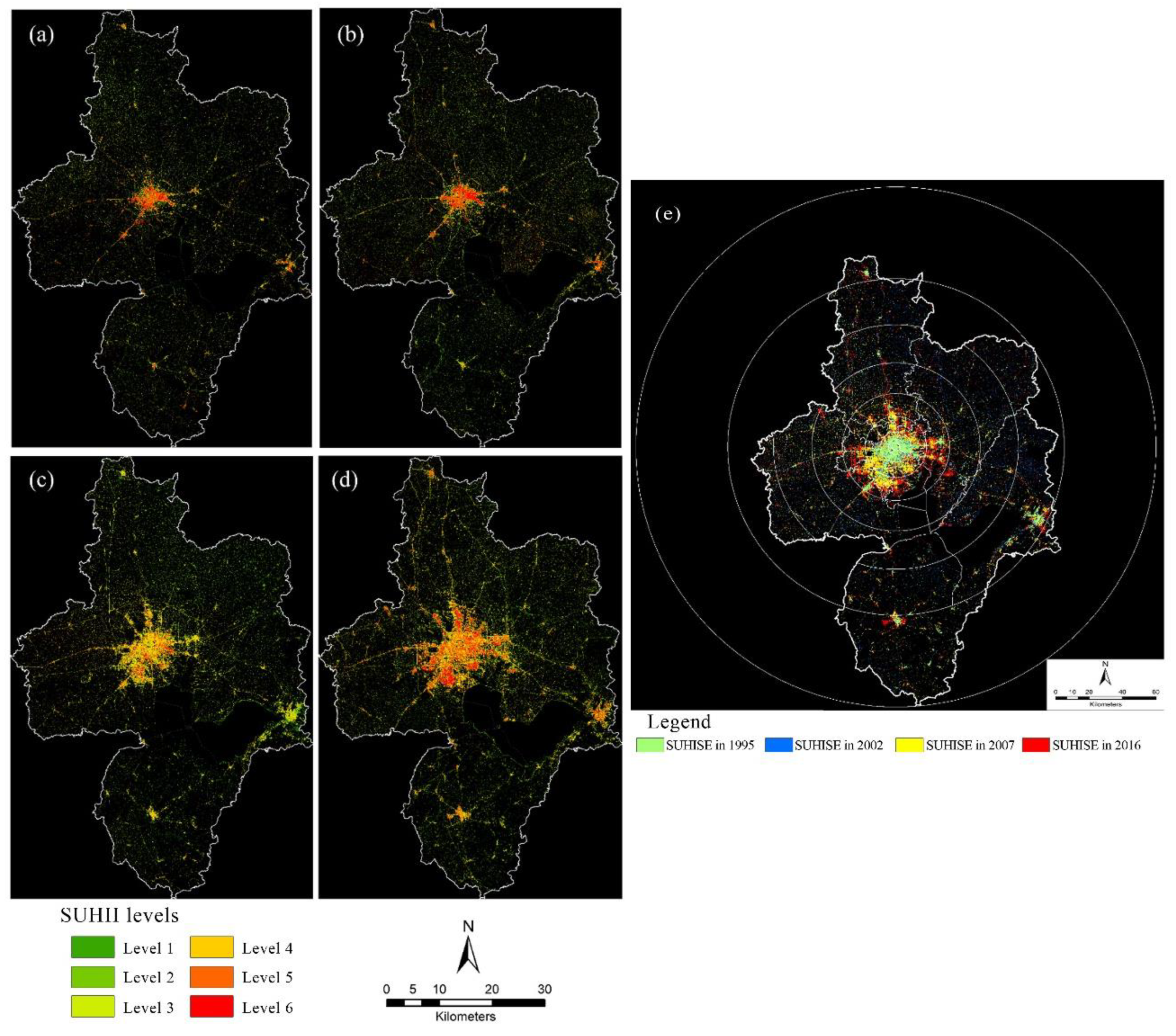
4.2. Change of Summertime SUHII and the Spatial Extent Influenced by SUHI Effect
4.3. Driving Factors Analysis of the Relationship between the LULC Change and SUHI Effect Indicators
5. Discussion
5.1. On the Relationship Between LULC Change and Summertime SUHI Effect
5.2. Implications for Sustainable Land Development of a Better Urban Thermal Environment
5.3. Limitations of This Study and Remarks
6. Conclusions
Author Contributions
Funding
Acknowledgments
Conflicts of Interest
Appendix A

| Developed Land | Forest | Water Body | Cropland | Bare Land | Pop_Density | SUHII | |
|---|---|---|---|---|---|---|---|
| Forest | −0.642 ** | ||||||
| Water body | −0.272 * | 0.576 ** | |||||
| Cropland | −0.580 ** | 0.692 ** | 0.965 ** | ||||
| Bare land | 0.650 ** | 0.478 ** | 0.484 ** | 0.430 ** | |||
| Pop_density | 0.484 ** | −0.609 ** | −0.654 ** | −0.769 ** | −0.372 * | ||
| SUHII | 0.611 ** | −0.579 ** | −0.602 ** | −0.710 ** | −0.234 * | 0.705 ** | |
| SUHISE | 0.578 ** | −0.634 ** | −0.659 ** | −0.785 ** | −0.362 ** | 0.980 ** | 0.788 ** |
References
- United Nations. 2018 Revision of World Urbanization Prospects. Available online: https://www.un.org/development/desa/publications/2018-revision-of-world-urbanization-prospects.html (accessed on 20 November 2018).
- Cai, Y.-B.; Li, H.-M.; Ye, X.-Y.; Zhang, H. Analyzing three-decadal patterns of land use/land cover change and regional ecosystem services at the landscape level: Case study of two coastal metropolitan regions, eastern China. Sustainability 2016, 8, 773. [Google Scholar] [CrossRef] [Green Version]
- Kim, J.J.; Ryu, J.H. Modeling Hydrological and Environmental Consequences of Climate Change and Urbanization in the Boise River Watershed, Idaho. J. Am. Water Resour. Assoc. 2019, 55, 133–153. [Google Scholar] [CrossRef] [Green Version]
- Dewan, A.M.; Yamaguchi, Y. Land use and land cover change in Greater Dhaka, Bangladesh: Using remote sensing to promote sustainable urbanization. Appl. Geogr. 2009, 29, 390–401. [Google Scholar] [CrossRef]
- King, R.S.; Scoggins, M.; Porras, A. Stream biodiversity is disproportionately lost to urbanization when flow permanence declines: Evidence from southwestern North America. Freshw. Sci. 2016, 35, 340–352. [Google Scholar] [CrossRef]
- Nguyen, H.H.; Recknagel, F.; Meyer, W. Effects of projected urbanization and climate change on flow and nutrient loads of a Mediterranean catchment in South Australia. Ecohydrol. Hydrobiol. 2019, 19, 279–288. [Google Scholar] [CrossRef]
- Mati, B.M.; Mutie, S.; Gadain, H.; Home, P.; Mtalo, F. Impacts of land-use/cover changes on the hydrology of the transboundary Mara River, Kenya/Tanzania. Lakes Reserv. Res. Manag. 2008, 13, 169–177. [Google Scholar] [CrossRef]
- Pickard, B.R.; Van Berkel, D.; Petrasova, A.; Meentemeyer, R.K. Forecasts of urbanization scenarios reveal trade-offs between landscape change and ecosystem services. Landsc. Ecol. 2017, 32, 617–634. [Google Scholar] [CrossRef]
- Reyers, B.; O’Farrell, P.J.; Cowling, R.M.; Egoh, B.N.; Le Maitre, D.C.; Vlok, J.H.J. Ecosystem services, land-cover change, and stakeholders: Finding a sustainable foothold for a semiarid biodiversity hotspot. Ecol. Soc. 2009, 14, 38. [Google Scholar] [CrossRef] [Green Version]
- McMichael, A.J.; Woodruff, R.E.; Hales, S. Climate change and human health: Present and future risks. Lancet 2006, 367, 858–869. [Google Scholar] [CrossRef]
- Jenerette, G.D.; Harlan, S.L.; Buyantuev, A.; Stefanov, W.L.; Declet-Barreto, J.; Ruddell, B.L.; Myint, S.E.; Kaplan, S.; Li, X. Micro-scale urban surface temperatures are related to land-cover features and residential heat related health impacts in Phoenix, AZ USA. Landsc. Ecol. 2016, 31, 745–760. [Google Scholar] [CrossRef]
- Luan, X.; Yu, Z.; Zhang, Y.; Wei, S.; Miao, X.; Huang, Z.Y.X.; Teng, S.N.; Xu, C. Remote Sensing and Social Sensing Data Reveal Scale-Dependent and System-Specific Strengths of Urban Heat Island Determinants. Remote Sens. 2020, 12, 391. [Google Scholar] [CrossRef] [Green Version]
- Georgescu, M.; Morefield, P.E.; Bierwagen, B.G.; Weaver, C.P. Urban adaptation can roll back warming of emerging megapolitan regions. Proc. Natl. Acad. Sci. USA 2014, 111, 2909–2914. [Google Scholar] [CrossRef] [PubMed] [Green Version]
- Liu, J.; Shao, Q.; Yan, X.; Fan, J.; Zhan, J.; Deng, X.; Kuang, W.; Huang, L. The climatic impacts of land use and land cover change compared among countries. J. Geogr. Sci. 2016, 26, 889–903. [Google Scholar] [CrossRef] [Green Version]
- Peng, J.; Jia, J.; Liu, Y.; Li, H.; Wu, J. Seasonal contrast of the dominant factors for spatial distribution of land surface temperature in urban areas. Remote Sens. Environ. 2018, 215, 255–267. [Google Scholar] [CrossRef]
- Polydoros, A.; Mavrakou, T.; Cartalis, C. Quantifying the trends in land surface temperature and surface urban heat island intensity in mediterranean cities in view of smart urbanization. Urban Sci. 2018, 2, 16. [Google Scholar] [CrossRef] [Green Version]
- Zhang, H.; Li, T.-T.; Liu, Y.; Han, J.-J.; Guo, Y.-J. Understanding the contributions of land parcel features to intra-surface urban heat island intensity and magnitude: Study on downtown Shanghai, China. Land Degrad. Dev. 2020. [Google Scholar] [CrossRef]
- Gill, S.; Handley, J.; Ennos, A.; Pauleit, S. Adapting Cities for Climate Change: The Role of the Green Infrastructure. Built Environ. 2007, 33, 115–133. [Google Scholar] [CrossRef] [Green Version]
- Daily, G. Nature’s Services: Societal Dependence on Natural Ecosystems; Island Press: Washington, DC, USA, 1997. [Google Scholar]
- Dissanayake, D.; Morimoto, T.; Murayama, Y.; Ranagalage, M. Impact of Landscape Structure on the Variation of Land Surface Temperature in Sub-Saharan Region: A Case Study of Addis Ababa Using Landsat Data (1986–2016). Sustainability 2019, 11, 2257. [Google Scholar] [CrossRef] [Green Version]
- Oke, T.R. City size and the urban heat island. Atmos. Environ. 1973, 7, 769–779. [Google Scholar] [CrossRef]
- Ren, C.Y.; Wu, D.T.; Dong, S.C. The influence of urbanization on the urban climate environment in Northwest China. Geogr. Res. Aust. 2006, 25, 233–241. [Google Scholar]
- China National People’s Congress. The 10th Five-Year Plan Outline of China’s for National Economic and Social Development. Available online: http://www.gov.cn/gongbao/content/2001/content_60699.htm (accessed on 1 November 2017).
- The State Council of China. The 11th Five-Year Planning for Great Western Development Strategy. Available online: http://xbkfs.ndrc.gov.cn/qyzc/200901/t20090118_256835.html (accessed on 1 November 2017).
- Wang, J.P.; Liu, J.; Du, J.S.; Zhang, X.; Xue, C.F.; Gao, W.Y. Interdecadal Variation of the Temperature and the Impact of Urban Growth on the Temperature in Xi’an Region. Clim. Environ. Res. 2009, 14, 434–444. [Google Scholar]
- Cai, Z.; Han, G.F. Assessing land surface temperature in the mountain city with different urban spatial form based on local climate zone scheme. Mt. Res. 2018, 4, 617–627. [Google Scholar]
- Zhao, H.; Zhang, H.; Miao, C.; Ye, X.; Min, M. Linking heat source–sink landscape patterns with analysis of urban heat islands: Study on the fast-growing Zhengzhou city in central China. Remote Sens. 2018, 10, 1268. [Google Scholar] [CrossRef] [Green Version]
- Voogt, J.A.; Oke, T.R. Thermal remote sensing of urban climates. Remote Sens. Environ. 2003, 86, 370–384. [Google Scholar] [CrossRef]
- Weng, Q. Thermal infrared remote sensing for urban climate and environmental studies: Methods, applications, and trends. ISPRS J. Photogramm. Remote Sens. 2009, 64, 335–344. [Google Scholar] [CrossRef]
- Adinna, E.N.; Christian, E.I.; Okolie, A.T. Assessment of urban heat island and possible adaptations in Enugu urban using landsat-ETM. J. Geogr. Reg. Plann. 2009, 2, 30–36. [Google Scholar]
- Keeratikasikorn, C.; Bonafoni, S. Urban heat island analysis over the land use zoning plan of Bangkok by means of landsat 8 imagery. Remote Sens. 2018, 10, 440. [Google Scholar] [CrossRef]
- Rosenzweig, C.; Solecki, W.D.; Parshall, L.; Lynn, B.; Cox, J.; Goldberg, R.; Hodges, S.; Gaffin, S.; Slosberg, R.B.; Savio, P.; et al. Mitigating New York City’s heat island: Integrating stakeholder perspectives and scientific evaluation. Bull. Am. Meteorol. Soc. 2009, 90, 1297–1312. [Google Scholar] [CrossRef]
- Simwanda, M.; Ranagalage, M.; Estoque, R.C.; Murayama, Y. Spatial analysis of surface urban heat islands in four rapidly growing African cities. Remote Sens. 2019, 11, 1645. [Google Scholar] [CrossRef] [Green Version]
- Rousta, I.; Sarif, M.O.; Gupta, R.D.; Olafsson, H.; Ranagalage, M.; Murayama, Y.; Zhang, H.; Mushore, T.D. Spatiotemporal analysis of land use/land cover and its effects on surface urban heat island using landsat data: A case study of metropolitan city Tehran (1988–2018). Sustainability 2018, 10, 4433. [Google Scholar] [CrossRef] [Green Version]
- Sodoudi, S.; Shahmohamadi, P.; Vollack, K.; Cubasch, U.; Che-Ani, A.I. Mitigating the urban heat island effect in megacity Tehran. Adv. Meteorol. 2014, 2014. [Google Scholar] [CrossRef]
- Lu, L.; Weng, Q.; Xiao, D.; Guo, H.; Li, Q.; Hui, W. Spatiotemporal Variation of Surface Urban Heat Islands in Relation to Land Cover Composition and Configuration: A Multi-Scale Case Study of Xi’an, China. Remote Sens. 2020, 12, 2713. [Google Scholar] [CrossRef]
- Huang, Q.; Huang, J.; Yang, X.; Fang, C.; Liang, Y. Quantifying the seasonal contribution of coupling urban land use types on Urban Heat Island using Land Contribution Index: A case study in Wuhan, China. Sustain. Cities Soc. 2019, 44, 666–675. [Google Scholar] [CrossRef]
- Qiao, Z.; Liu, L.; Qin, Y.; Xu, X.; Wang, B.; Liu, Z. The Impact of Urban Renewal on Land Surface Temperature Changes: A Case Study in the Main City of Guangzhou, China. Remote Sens. 2020, 12, 794. [Google Scholar] [CrossRef] [Green Version]
- Singh, P.; Kikon, N.; Verma, P. Impact of land use change and urbanization on urban heat island in Lucknow city, Central India. A remote sensing based estimate. Sustain. Cities Soc. 2017, 32, 100–114. [Google Scholar] [CrossRef]
- Tariq, A.; Riaz, I.; Ahmad, Z.; Yang, B.; Amin, M.; Kausar, R.; Andleeb, S.; Farooqi, M.A.; Rafiq, M. Land surface temperature relation with normalized satellite indices for the estimation of spatio-temporal trends in temperature among various land use land cover classes of an arid Potohar region using Landsat data. Environ. Earth Sci. 2020, 79, 40. [Google Scholar] [CrossRef]
- Yang, C.; He, X.; Yan, F.; Yu, L.; Bu, K.; Yang, J.; Chang, L.; Zhang, S. Mapping the Influence of Land Use/Land Cover Changes on the Urban Heat Island Effect—A Case Study of Changchun, China. Sustainability 2017, 9, 312. [Google Scholar] [CrossRef] [Green Version]
- Zhang, Y.; Sun, L. Spatial-temporal impacts of urban land use land cover on land surface temperature: Case studies of two Canadian urban areas. Int. J. Appl. Earth Obs. 2019, 75, 171–181. [Google Scholar] [CrossRef]
- Liu, Y.; Peng, J.; Wang, Y. Application of partial least squares regression in detecting the important landscape indicators determining urban land surface temperature variation. Landsc. Ecol. 2018, 33, 1133–1145. [Google Scholar] [CrossRef]
- Zhang, H.; Qi, Z.F.; Ye, X.-Y.; Cai, Y.B.; Ma, W.C.; Chen, M.-N. Analysis of land use/land cover change, population shift, and their effects on spatiotemporal patterns of urban heat islands in metropolitan Shanghai, China. Appl. Geogr. 2013, 44, 121–133. [Google Scholar] [CrossRef]
- China Meterological Administration (CMA). The Increasing Trends of Hot Cities in China. Available online: http://www.cma.gov.cn/2011xwzx/2011xqhbh/2011xdtxx/201208/t20120816_182112.html (accessed on 11 November 2017).
- Hefei Municipal Government. Urban Master Planning of Hefei (2011–2020); Hefei Municipal Government: Hefei, China, 2012.
- Hefei Municipal Government. Overall Plan for Land Utilization of Hefei (2006–2020); Hefei Municipal Government: Hefei, China, 2012.
- Hefei Municipal Statistics Bureau. The 2017 Report of Demographic Census in Hefei. Available online: http://tjj.hefei.gov.cn/8726/8730/201802/t20180223_2481649.html (accessed on 5 September 2019).
- USGS. Available online: https://www.usgs.gov/centers/eros/science/usgs-eros-archive-landsat-archives-landsat-8-oli-operational-land-imager-and?qt-science_center_objects=0#qt-science_center_objects (accessed on 1 August 2019).
- Anhui Provincial Statistics Bureau. The Annual Statistical Yearbook of Anhui Province. Available online: http://tjj.ah.gov.cn/tjjweb/web/tjnj_view.jsp?strColId=13787135717978521&_index=1 (accessed on 3 September 2019).
- Hefei Municipal Statistics Bureau. The Annual Statistical Yearbook of Hefei. Available online: http://tjj.hefei.gov.cn/8688/8689/18nj/ (accessed on 5 September 2018).
- China National Committee of Agricultural Divisions. Technical Regulation of Investigation on Land Use Status; Surveying and Mapping Publishing House: Beijing, China, 1984.
- Chen, D.; Stow, D. The effect of training strategies on supervised classification at different spatial resolutions. Photogramm. Eng. Remote Sens. 2002, 68, 1155–1162. [Google Scholar]
- Jassen, L.I.F.; Frans, J.M.; Wel, V.D. Accuracy assessment of satellite derived land-cover data: A review. photogramm. Eng. Remote Sens. 1994, 60, 410–432. [Google Scholar]
- Song, C.; Woodcock, C.E.; Seto, K.C.; Lenney, M.P.; Macomber, S.A. Classification and change detection using Landsat TM data: When and how to correct atmospheric effects? Remote Sens. Environ. 2001, 75, 230–244. [Google Scholar] [CrossRef]
- Weng, Q. A remote sensing-GIS evaluation of urban expansion and its impact on surface temperature in the Zhujiang Delta, China. Int. J. Remote Sens. 2001, 22, 1999–2014. [Google Scholar]
- Malaret, E.; Bartolucci, L.A.; Lozano, D.F.; Anuta, P.E.; McGillem, C.D. Landsat-4 and Landsat-5 Thematic Mapper data quality analysis. Photogramm. Eng. Remote Sens. 1985, 51, 1407–1416. [Google Scholar]
- Barsi, J.A.; Schott, J.R.; Hook, S.J.; Raqueno, N.G.; Markham, B.L.; Radocinski, R.G. Landsat-8 Thermal Infrared Sensor (TIRS) vicarious radiometric calibration. Remote Sens. 2014, 6, 11607–11626. [Google Scholar] [CrossRef] [Green Version]
- Montanaro, M.; Gerace, A.; Lunsford, A.; Reuter, D. Stray light artifacts in imagery from the Landsat 8 thermal infrared sensor. Remote Sens. 2014, 6, 10435–10456. [Google Scholar] [CrossRef] [Green Version]
- Department of the Interior/U.S. Geological Survey (DOI/USGS). The Landsat 8 (L8) Data Users Handbook (Version 4.0). EROS Sioux Falls, South Dakota. 2019. Available online: https://prd-wret.s3-us-west-2.amazonaws.com/assets/palladium/production/atoms/files/LSDS_1574_L8_Data_Users_Handbook_v4.pdf (accessed on 12 May 2019).
- Sobrino, J.A.; Jiménez-Muñoz, J.C.; Paolini, L. Land surface temperature retrieval from Landsat TM 5. Remote Sens. Environ. 2004, 90, 434–440. [Google Scholar] [CrossRef]
- Carlson, T.N.; Ripley, D.A. On the relation between NDVI, fractional vegetation cover, and leaf area index. Remote Sens. Environ. 1997, 62, 241–252. [Google Scholar] [CrossRef]
- Artis, D.A.; Carnahan, W.H. Survey of emissivity variability in thermography of urban areas. Remote Sens. Environ. 1982, 12, 313–329. [Google Scholar] [CrossRef]
- Yang, Y.J.; Wu, B.W.; Shi, C.E.; Zhang, J.H.; Li, Y.B.; Tang, W.A.; Wen, H.Y.; Zhang, H.Q.; Shi, T. Impacts of urbanization and station-relocation on surface air temperature series in Anhui Province, China. Pure Appl. Geophys. 2013, 170, 1969–1983. [Google Scholar] [CrossRef]
- Stewart, I.D.; Oke, T.R. Local Climate Zones for Urban Temperature Studies. Bull. Am. Meteorol. Soc. 2012, 93, 1879–1900. [Google Scholar] [CrossRef]
- Abdi, H. Partial least squares regression and projection on latent structure regression (pls regression). Wiley Interdiplinary Rev. Comput. Stats 2010, 2, 97–106. [Google Scholar] [CrossRef]
- R Core Team. R: A Language and Environment for Statistical Computing. R Foundation for Statistical Computing, Vienna, Austria. 2019. Available online: https://www.R-project.org/ (accessed on 1 May 2019).
- Mevik, B.-H.; Wehrens, R. The pls package: Principal component and partial least squares regression in R. J. Stat. Softw. 2007, 18, 1–24. [Google Scholar] [CrossRef] [Green Version]
- Weng, Q.; Lu, D.; Schubring, J. Estimation of land surface temperature–vegetation abundance relationship for urban heat island studies. Remote Sens. Environ. 2004, 89, 467–483. [Google Scholar] [CrossRef]
- Xu, H. Analysis of impervious surface and its impact on urban heat environment using the normalized difference impervious surface index (NDISI). Photogramm. Eng. Remote Sens. 2010, 76, 557–565. [Google Scholar] [CrossRef]
- Buyantuyev, A.; Wu, J. Urban heat islands and landscape heterogeneity: Linking spatiotemporal variations in surface temperatures to land-cover and socioeconomic patterns. Landsc. Ecol. 2010, 25, 17–33. [Google Scholar] [CrossRef]
- Guo, Y.J.; Han, J.J.; Zhao, X.; Dai, X.Y.; Zhang, H. Understanding the Role of Optimized Land Use/Land Cover Components in Mitigating Summertime Intra-Surface Urban Heat Island Effect: A Study on Downtown Shanghai, China. Energies 2020, 13, 1678. [Google Scholar] [CrossRef] [Green Version]
- Tang, J.; Di, L.; Xiao, J.; Lu, D.; Zhou, Y. Impacts of land use and socioeconomic patterns on urban heat Island. Int. J. Remote Sens. 2017, 38, 3445–3465. [Google Scholar] [CrossRef]
- Cai, Z. The strategic planning for spatial development of Hefei City. Urban Plann. Newsrep. 2005, 14–15. [Google Scholar]
- Huang, Q.H.; Li, M.C.; Liu, Y.X.; Hu, W.; Liu, M.; Chen, Z.J.; Li, F.X. Using construction expansion regulation zones to manage urban growth in Hefei City, China. J. Urban Plan. Dev. 2012, 139, 62–69. [Google Scholar] [CrossRef]
- Bonafoni, S.; Anniballe, R.; Gioli, B.; Toscano, P. Downscaling Landsat land surface temperature over the urban area of Florence. Eur. J. Remote Sens. 2016, 49, 553–569. [Google Scholar] [CrossRef]
- Zhang, H.; Jing, X.M.; Chen, J.Y.; Li, J.J.; Schwegler, B. Characterizing urban fabric properties and their thermal effect using QuickBird image and Landsat 8 thermal infrared (TIR) Data: The case of downtown Shanghai, China. Remote Sens. 2016, 8, 541. [Google Scholar] [CrossRef] [Green Version]
- Li, Y.Y.; Deng, Y.Y.; Chen, Y.S.; Zhang, H. Characterization of Urban Green Space Thermal Environmental Effects Based on Satellite Remote Sensing: A Case Study of Hefei, China. Ecol. Environ. Sci. 2018, 27, 40–49. [Google Scholar]


| LULC Category | Description |
|---|---|
| Developed land | Urban and rural settlements, mainly including residences, commercial centers, economic development zone, industrial zones, college towns, railways, and highways |
| Forest | Mainly including natural and artificial woodlands, cropland shelterbelts, forest nurseries, and scrublands |
| Cropland | Paddy fields, fallow lands after harvest, drylands, and orchards |
| Water body | Lakes, rivers, ponds, reservoirs, fishponds, dikes, permanent and seasonal wetlands |
| Bare land | Bare rocks, quarries, mines, and vacant lands for urban development. |
| Buffer Distance (km) | Description |
|---|---|
| 0–1.5 | The city core of downtown Hefei. |
| 1.5–3.0 | The urban area between the inner and the first ring roads. |
| 3.0–6.0 | The urban area between the first and second ring roads. |
| 6.0–12.0 | The urban area with intensive settlements, industrial parks, old airports, reservoirs, and national forest parks. |
| 12.0–21.0 | The rapidly urbanizing areas with intensive settlements, industrial parks, college towns, and new urban areas. |
| 21.0–33.0 | The rural areas with sparsely distributed towns and villages along with the traffic. This zonal buffer is characterized by cropland, Chao lake, reservoir, national forest park, a new airport, and river network. |
| 33.0–48.0 | The low-density developed rural areas with sparsely distributed towns and villages. This zonal buffer is characterized by cropland, Chao lake, hilly and mountainous terrain, and river network. |
| 48.0–66.0 | The low-density developed rural areas with sparsely distributed towns and villages. Aside from the well-developed urban area of Chaohu City, this zonal buffer is characterized by cropland and river networks. |
| >66.0 | The low-density developed rural areas with sparsely distributed towns and villages. Aside from the well-developed urban area of Lujiang county in the south and Changfeng county in the east, this zonal buffer is characterized by hilly and mountainous terrain, dikes, and river network. |
| SUHII | SUHISE | |||
|---|---|---|---|---|
| Coefficients | Standardized Coefficients | Coefficients | Standardized Coefficients | |
| Constant | 6.724 | 0.000 | 53.813 | 0.000 |
| Developed land | 0.029 | 0.627 | 0.457 | 0.434 |
| Forest | −0.201 | −0.104 | −0.286 | −0.031 |
| Water body | −0.065 | −0.160 | −3.735 | −0.085 |
| Cropland | −0.050 | −1.016 | −0.579 | −0.518 |
| Bare land | 0.214 | 0.221 | 0.261 | 0.012 |
| Pop_density | 0.001 | 0.098 | 0.000 | 0.038 |
| Summary statistics | F4,31 = 19.499, p < 0.05 R2 = 0.613 | F4,31 = 47.290, p < 0.05 R2 = 0.798 | ||
© 2020 by the authors. Licensee MDPI, Basel, Switzerland. This article is an open access article distributed under the terms and conditions of the Creative Commons Attribution (CC BY) license (http://creativecommons.org/licenses/by/4.0/).
Share and Cite
Li, Y.-y.; Liu, Y.; Ranagalage, M.; Zhang, H.; Zhou, R. Examining Land Use/Land Cover Change and the Summertime Surface Urban Heat Island Effect in Fast-Growing Greater Hefei, China: Implications for Sustainable Land Development. ISPRS Int. J. Geo-Inf. 2020, 9, 568. https://0-doi-org.brum.beds.ac.uk/10.3390/ijgi9100568
Li Y-y, Liu Y, Ranagalage M, Zhang H, Zhou R. Examining Land Use/Land Cover Change and the Summertime Surface Urban Heat Island Effect in Fast-Growing Greater Hefei, China: Implications for Sustainable Land Development. ISPRS International Journal of Geo-Information. 2020; 9(10):568. https://0-doi-org.brum.beds.ac.uk/10.3390/ijgi9100568
Chicago/Turabian StyleLi, Ying-ying, Yu Liu, Manjula Ranagalage, Hao Zhang, and Rui Zhou. 2020. "Examining Land Use/Land Cover Change and the Summertime Surface Urban Heat Island Effect in Fast-Growing Greater Hefei, China: Implications for Sustainable Land Development" ISPRS International Journal of Geo-Information 9, no. 10: 568. https://0-doi-org.brum.beds.ac.uk/10.3390/ijgi9100568