Rainfall-Induced Shallow Landslide Susceptibility Mapping at Two Adjacent Catchments Using Advanced Machine Learning Algorithms


Abstract
:
1. Introduction
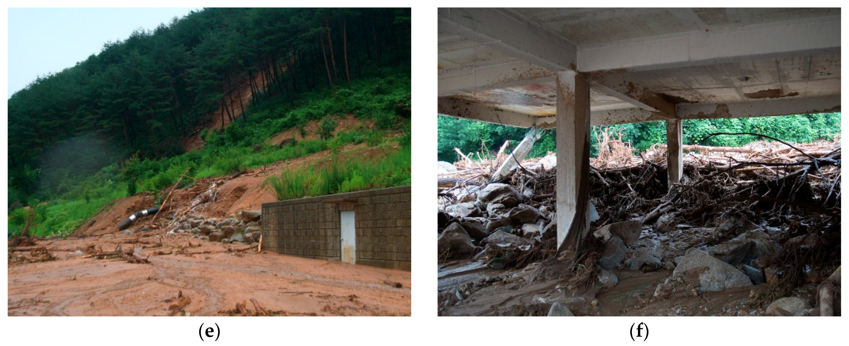
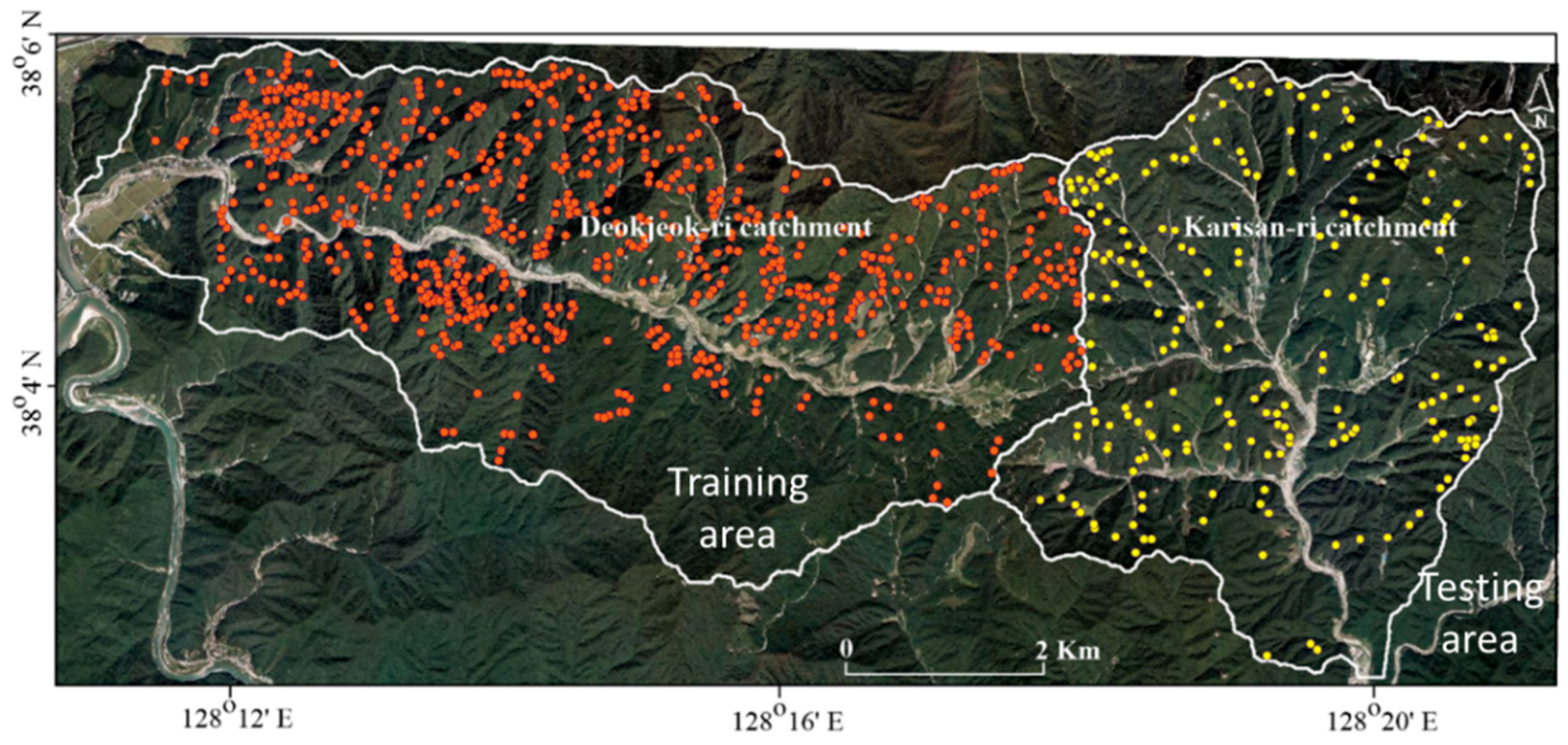
2. Description of Study Area
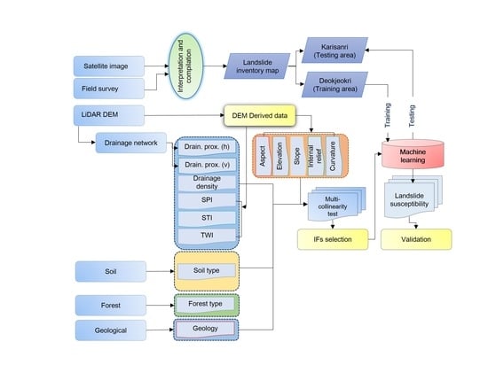
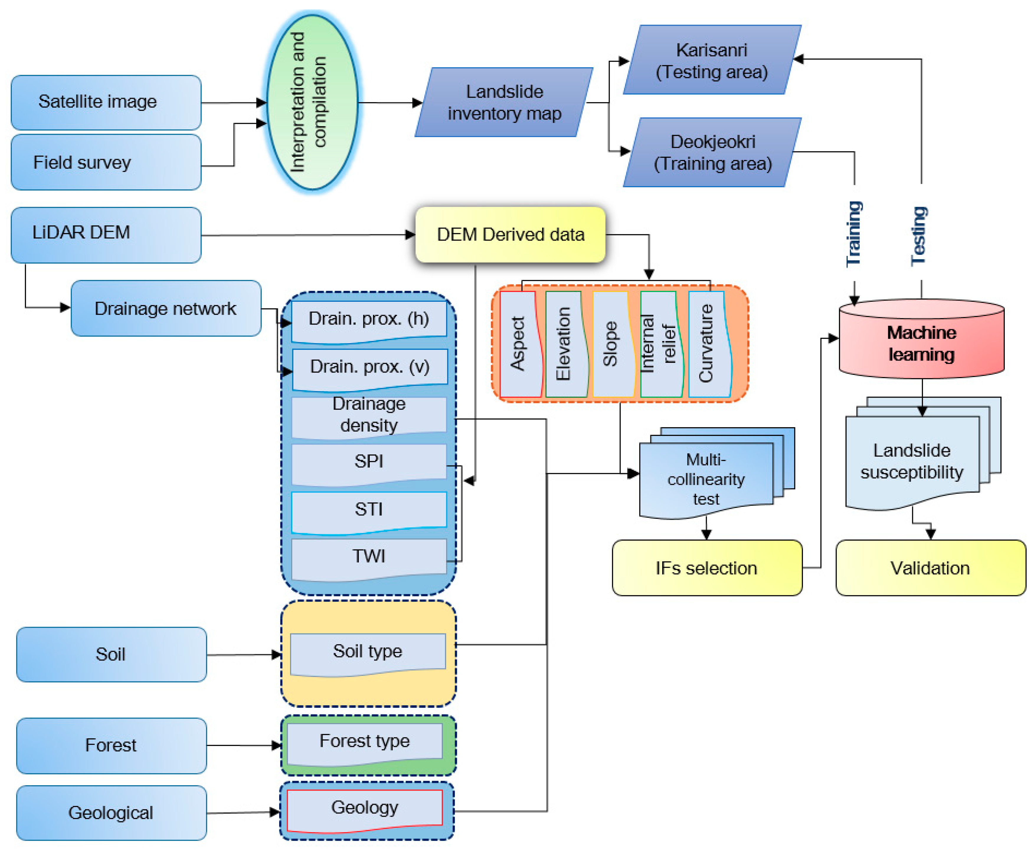
3. The Collected Dataset and Methods
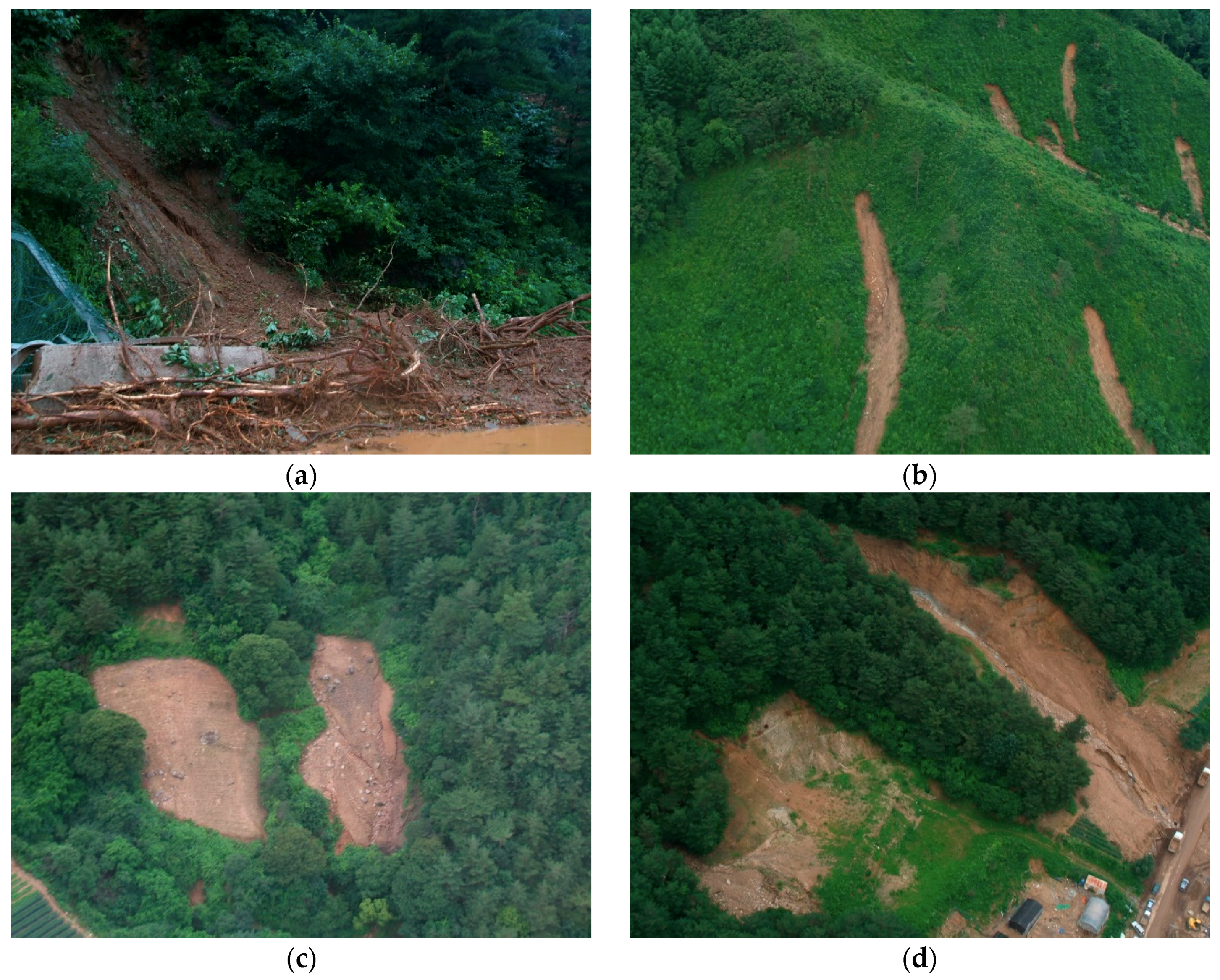
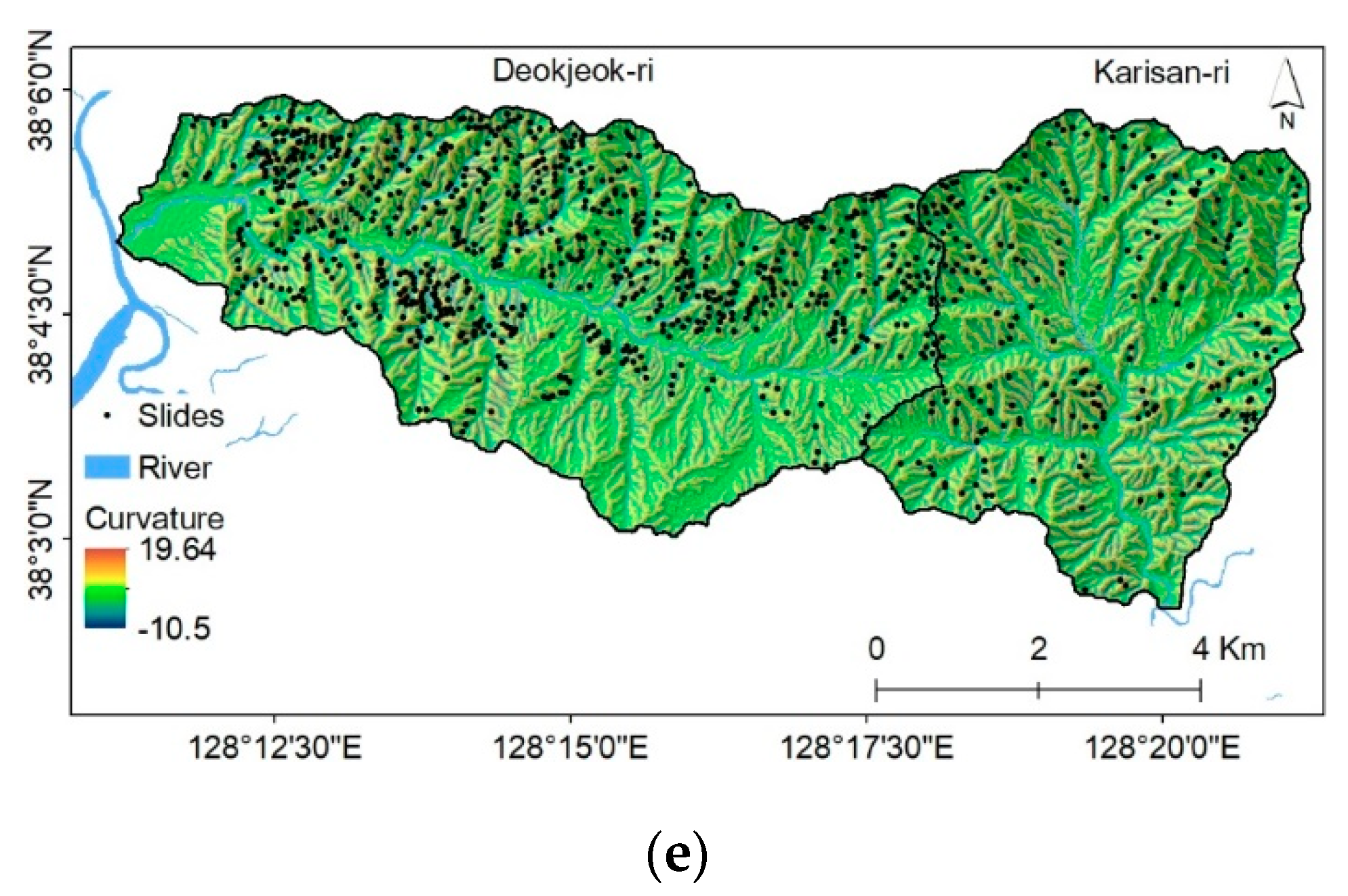
3.1. Landslide Inventory
3.2. Landslide Influencing Factor (IF)
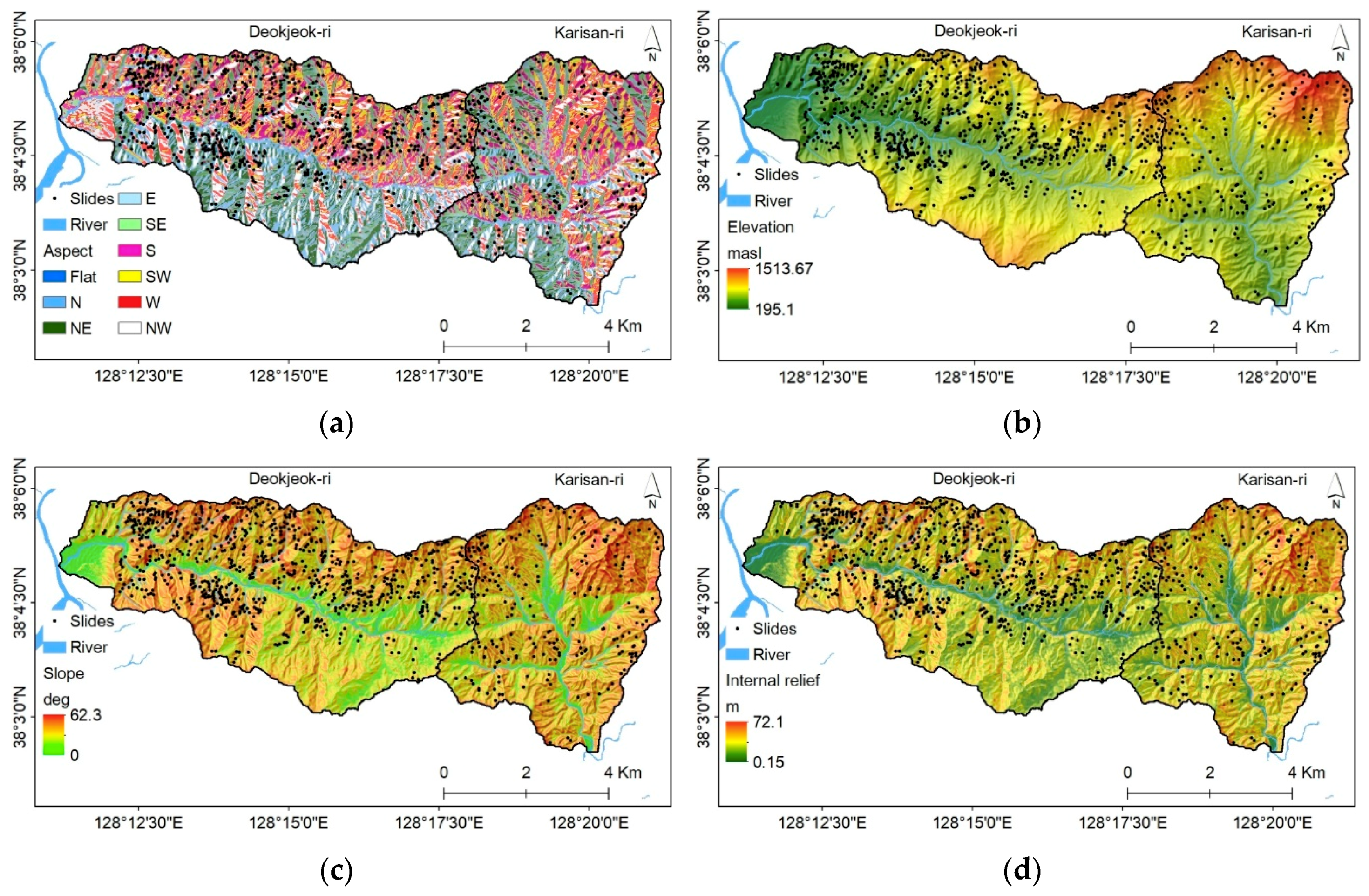
3.2.1. Topographic Factors
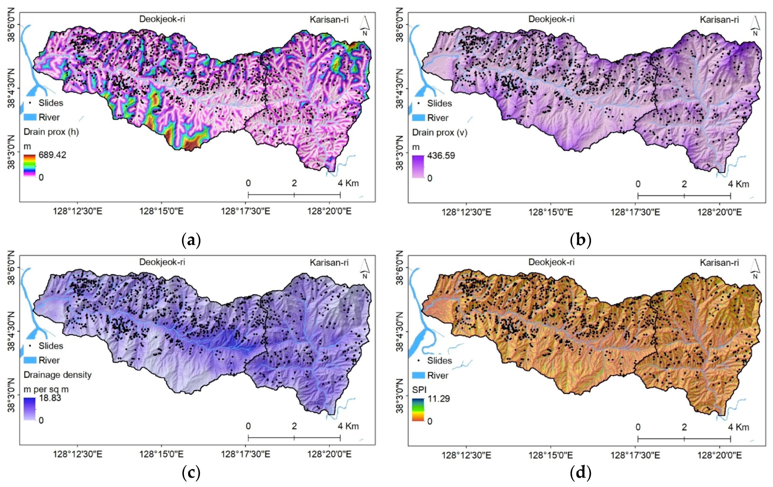
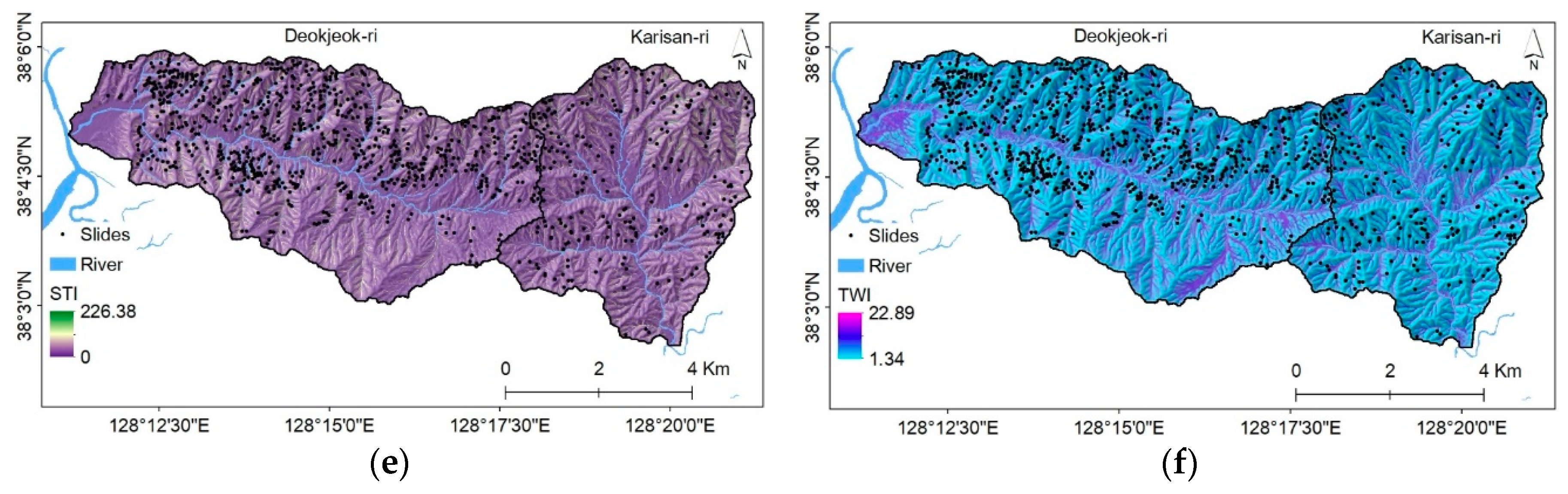
3.2.2. Hydrologic Factors
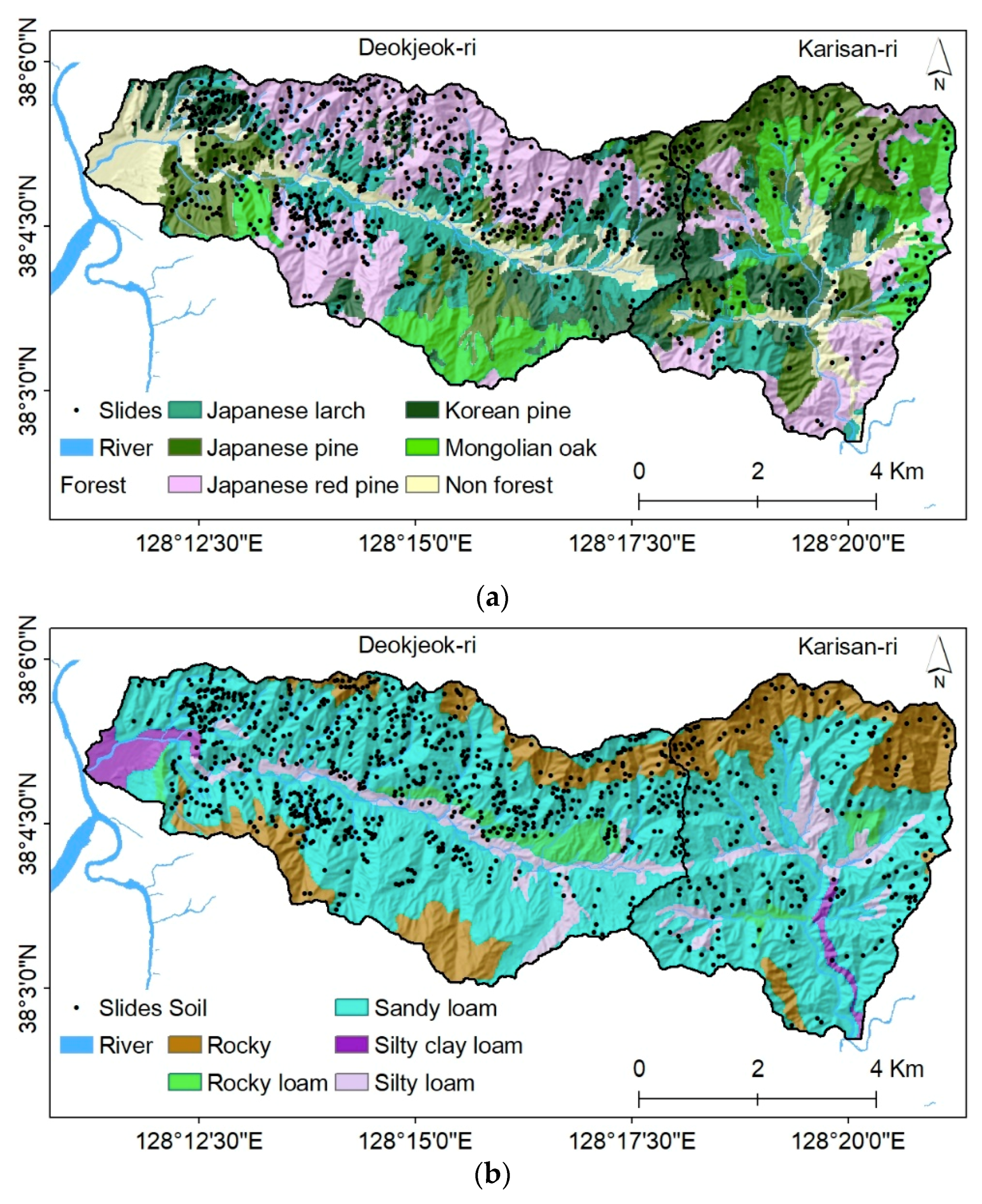
3.2.3. Forest and Soil Factors
3.2.4. Geologic Factor
3.3. Modeling Approaches
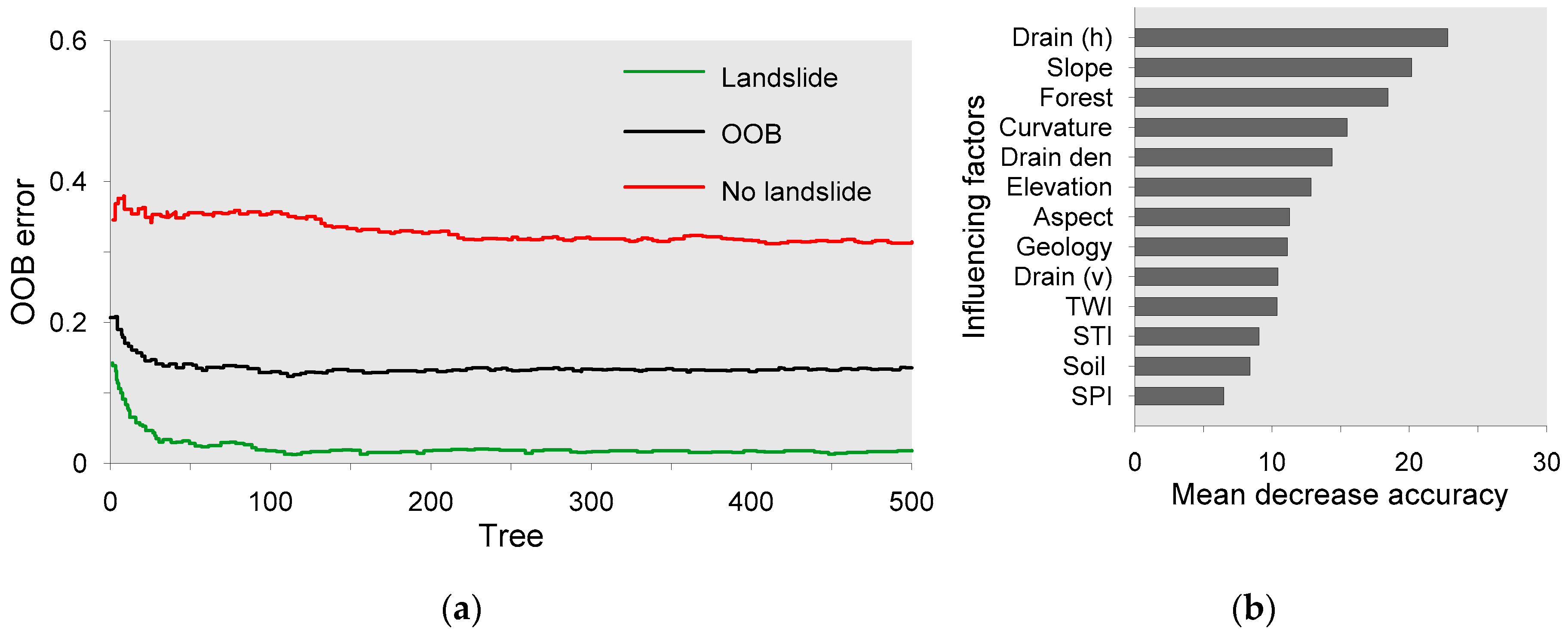
3.3.1. Random Forest (RF)
3.3.2. Extreme Gradient Boosting (XGBoost)
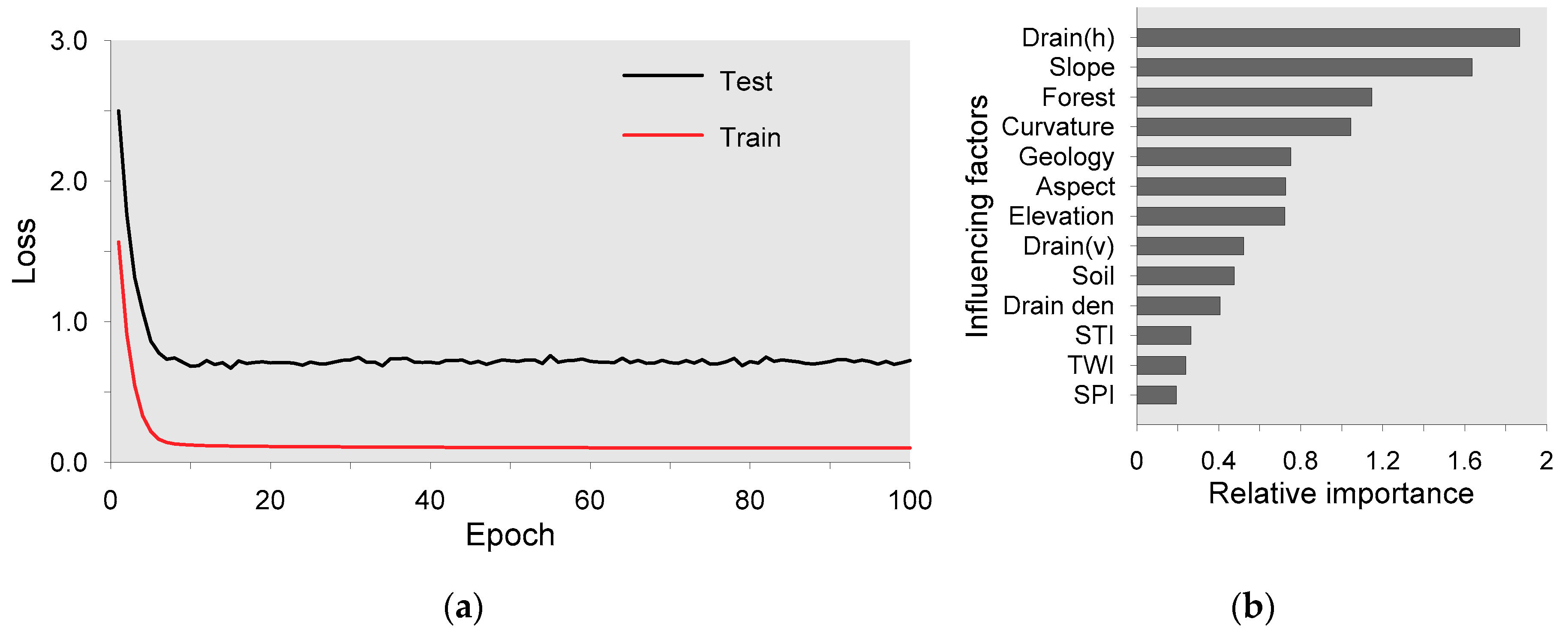
3.3.3. Deep Neural Network (DNN)
4. Results and Analysis
4.1. Selection of IFs
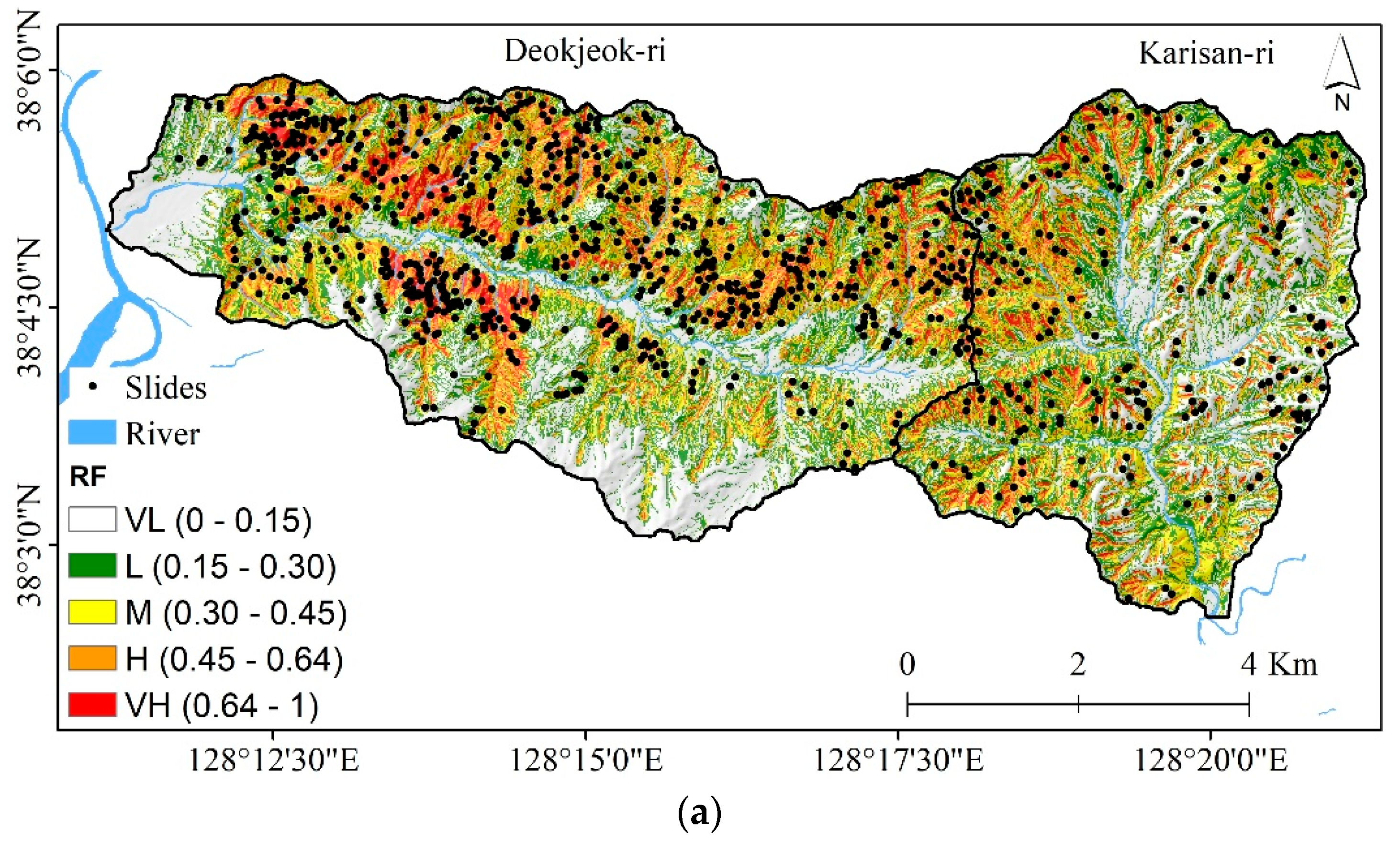
4.2. Application of RF in Landslide Susceptibility Mapping
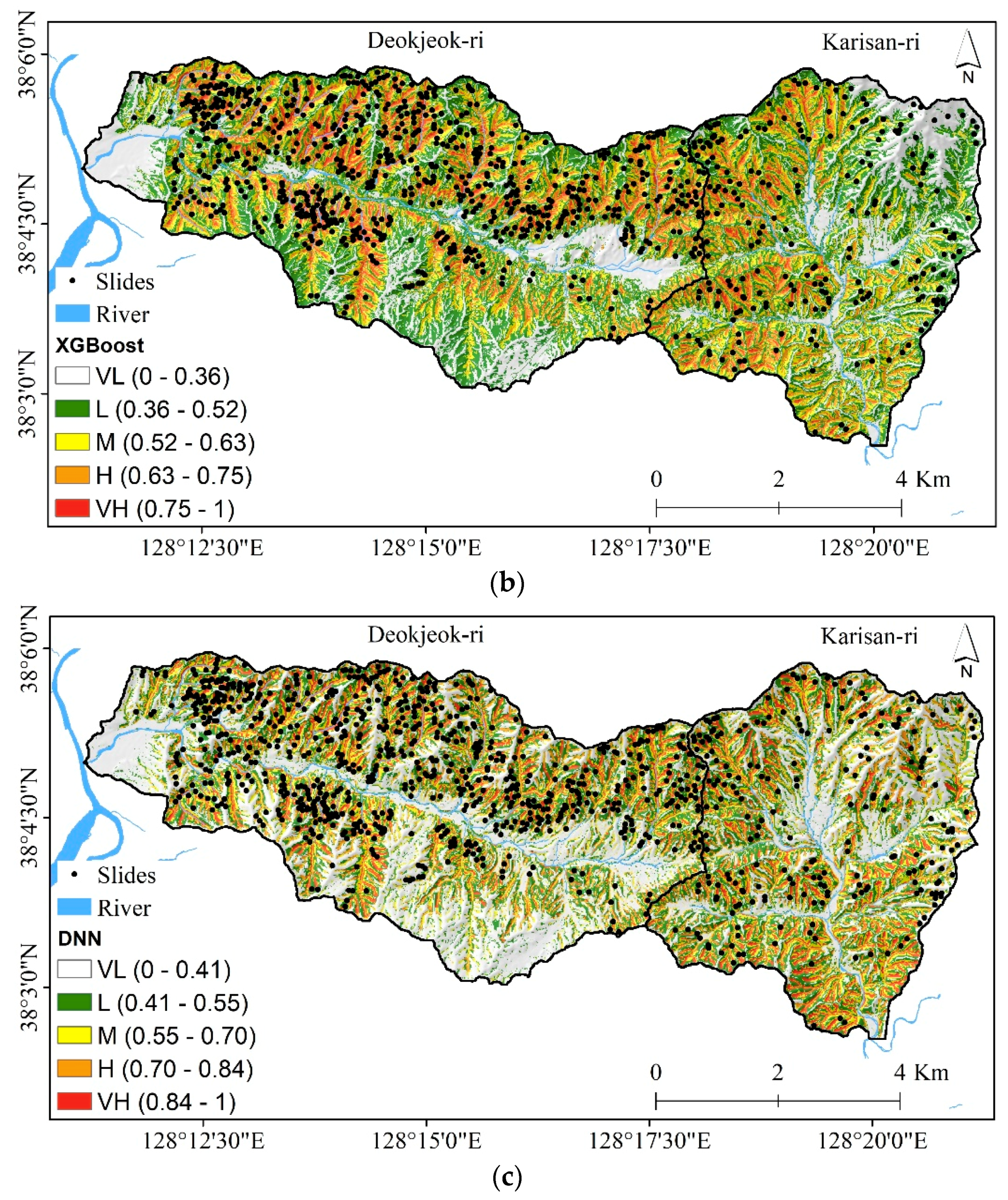
4.3. Application of XGBost in Landslide Susceptibility Mapping
4.4. Application of DNN in Landslide Susceptibility Mapping
4.5. Evaluation Measures
5. Discussion
6. Conclusions
Author Contributions
Funding
Acknowledgments
Conflicts of Interest
References
- Chung, Y.-S.; Yoon, M.-B.; Kim, H.-S. On Climate Variations and Changes Observed in South Korea. Clim. Chang. 2004, 66, 151–161. [Google Scholar] [CrossRef]
- Kim, Y.-T.; Lee, J.-S. Slope Stability Characteristic of Unsaturated Weathered Granite Soil in Korea considering Antecedent Rainfall. Geo Congr. 2013 2013, 349–401. [Google Scholar] [CrossRef]
- Miles, S.B.; Keefer, D.K. Evaluation of seismic slope-performance models using a regional case study. Environ. Eng. Geosci. 2000, 6, 25–39. [Google Scholar] [CrossRef]
- Tarolli, P.; Tarboton, D.G. A new method for determination of most likely landslide initiation points and the evaluation of digital terrain model scale in terrain stability mapping. Hydrol. Earth Syst. Sci. 2006, 10, 663–667. [Google Scholar] [CrossRef] [Green Version]
- Iida, T. A hydrological method of estimation of the topographic effect on the saturated throughflow. Jpn. Geomorph. Union Trans. 1984, 5, 1–12. [Google Scholar]
- Keefer, D.K. Investigating landslides caused by earthquakes—A historical review. Surv. Geophys. 2002, 23, 473–510. [Google Scholar] [CrossRef]
- Moore, J.G.; Clague, D.A.; Holcomb, R.T.; Lipman, P.W.; Normark, W.R.; Torresan, M.E. Prodigious submarine landslides on the Hawaiian Ridge. J. Geophys. Res. 1989, 94, 17465–17484. [Google Scholar] [CrossRef] [Green Version]
- Brabb, E.E. Innovative Approaches to Landslide Hazard Mapping. In Proceedings of the 4th International Symposium on Landslides, Toronto, ON, Canada, 23–31 August 1984; pp. 307–324. [Google Scholar]
- Furlani, S.; Ninfo, A. Is the present the key to the future? Earth-Sci. Rev. 2015, 142, 38–46. [Google Scholar] [CrossRef]
- Carrara, A.; Cardinali, M.; Detti, R.; Guzzetti, F.; Pasqui, V.; Reichenbach, P. GIS techniques and statistical models in evaluating landslide hazard. Earth Surf. Process. Landf. 1991, 16, 427–445. [Google Scholar] [CrossRef]
- Chung, C.-J.F.; Fabbri, A.G. Validation of Spatial Prediction Models for Landslide Hazard Mapping. Nat. Hazards 2003, 30, 451–472. [Google Scholar] [CrossRef]
- Corominas, J.; van Westen, C.; Frattini, P.; Cascini, L.; Malet, J.-P.; Fotopoulou, S.; Catani, F.; Van Den Eeckhaut, M.; Mavrouli, O.; Agliardi, F.; et al. Recommendations for the quantitative analysis of landslide risk. Bull. Eng. Geol. Environ. 2013, 73, 209–263. [Google Scholar] [CrossRef]
- Reichenbach, P.; Rossi, M.; Malamud, B.D.; Mihir, M.; Guzzetti, F. A review of statistically-based landslide susceptibility models. Earth-Sci. Rev. 2018, 180, 60–91. [Google Scholar] [CrossRef]
- Dai, F.; Lee, C. Landslide characteristics and slope instability modeling using GIS, Lantau Island, Hong Kong. Geomorphology 2002, 42, 213–228. [Google Scholar] [CrossRef]
- Shrestha, S.; Kang, T.-S.; Choi, J.C. Assessment of co-seismic landslide susceptibility using LR and ANCOVA in Barpak region, Nepal. J. Earth Syst. Sci. 2018, 127, 38. [Google Scholar] [CrossRef] [Green Version]
- Aleotti, P.; Chowdhury, R. Landslide hazard assessment: Summary review and new perspectives. Bull. Eng. Geol. Environ. 1999, 58, 21–44. [Google Scholar] [CrossRef]
- Ko Ko, C.; Flentje, P.; Chowdhury, R. Quantitative Landslide Hazard and Risk Assessment: A Case Study. Q. J. Eng. Geol. Hydrogeol. 2003, 36, 261–272. [Google Scholar] [CrossRef]
- Pradhan, A.M.S.; Kim, Y.T. Relative effect method of landslide susceptibility zonation in weathered granite soil: A case study in Deokjeok-ri Creek, South Korea. Nat. Hazards 2014, 72, 1189–1217. [Google Scholar] [CrossRef]
- Pradhan, A.M.S.; Dawadi, A.; Kim, Y.T. Use of different bivariate statistical landslide susceptibility methods: A case study of Khulekhani watershed, Nepal. J. Nepal Geol. Soc. 2012, 44, 1–12. [Google Scholar] [CrossRef]
- Hong, H.; Liu, J.; Bui, D.T.; Pradhan, B.; Acharya, T.D.; Pham, B.T.; Zhu, A.-X.; Chen, W.; Ahmad, B. Bin Landslide susceptibility mapping using J48 Decision Tree with AdaBoost, Bagging and Rotation Forest ensembles in the Guangchang area (China). CATENA 2018, 163, 399–413. [Google Scholar] [CrossRef]
- Pourghasemi, H.; Gayen, A.; Park, S.; Lee, C.-W.; Lee, S.; Pourghasemi, H.R.; Gayen, A.; Park, S.; Lee, C.-W.; Lee, S. Assessment of Landslide-Prone Areas and Their Zonation Using Logistic Regression, LogitBoost, and NaïveBayes Machine-Learning Algorithms. Sustainability 2018, 10, 3697. [Google Scholar] [CrossRef] [Green Version]
- Thai Pham, B.; Prakash, I.; Dou, J.; Singh, S.K.; Trinh, P.T.; Trung Tran, H.; Minh Le, T.; Tran, V.P.; Kim Khoi, D.; Shirzadi, A.; et al. A Novel Hybrid Approach of Landslide Susceptibility Modeling Using Rotation Forest Ensemble and Different Base Classifiers. Geocarto Int. 2018, 14, 1–38. [Google Scholar] [CrossRef]
- Pham, B.T.; Nguyen, M.D.; Bui, K.-T.T.; Prakash, I.; Chapi, K.; Bui, D.T. A novel artificial intelligence approach based on Multi-layer Perceptron Neural Network and Biogeography-based Optimization for predicting coefficient of consolidation of soil. CATENA 2019, 173, 302–311. [Google Scholar] [CrossRef]
- Kornejady, A.; Pourghasemi, H.R.; Afzali, S.F. Presentation of RFFR New Ensemble Model for Landslide Susceptibility Assessment in Iran; Springer: Cham, Switzerland, 2019; pp. 123–143. [Google Scholar]
- Nhu, V.H.; Hoang, N.D.; Nguyen, H.; Ngo, P.T.T.; Thanh Bui, T.; Hoa, P.V.; Samui, P.; Tien Bui, D. Effectiveness assessment of Keras based deep learning with different robust optimization algorithms for shallow landslide susceptibility mapping at tropical area. Catena 2020, 188, 104458. [Google Scholar] [CrossRef]
- Knudby, A.; Brenning, A.; LeDrew, E. New approaches to modelling fish–habitat relationships. Ecol. Modell. 2010, 221, 503–511. [Google Scholar] [CrossRef]
- Falah, F.; Ghorbani Nejad, S.; Rahmati, O.; Daneshfar, M.; Zeinivand, H. Applicability of generalized additive model in groundwater potential modelling and comparison its performance by bivariate statistical methods. Geocarto Int. 2017, 32, 1069–1089. [Google Scholar] [CrossRef]
- Arabameri, A.; Yamani, M.; Pradhan, B.; Melesse, A.; Shirani, K.; Tien Bui, D. Novel ensembles of COPRAS multi-criteria decision-making with logistic regression, boosted regression tree, and random forest for spatial prediction of gully erosion susceptibility. Sci. Total Environ. 2019, 688, 903–916. [Google Scholar] [CrossRef]
- Darabi, H.; Choubin, B.; Rahmati, O.; Torabi Haghighi, A.; Pradhan, B.; Kløve, B. Urban flood risk mapping using the GARP and QUEST models: A comparative study of machine learning techniques. J. Hydrol. 2019, 569, 142–154. [Google Scholar] [CrossRef]
- Kavzoglu, T.; Colkesen, I.; Sahin, E.K. Machine Learning Techniques in Landslide Susceptibility Mapping: A Survey and a Case Study; Springer: Cham, Switzerland, 2019; pp. 283–301. [Google Scholar]
- Nguyen, V.; Pham, B.; Vu, B.; Prakash, I.; Jha, S.; Shahabi, H.; Shirzadi, A.; Ba, D.; Kumar, R.; Chatterjee, J.; et al. Hybrid Machine Learning Approaches for Landslide Susceptibility Modeling. Forests 2019, 10, 157. [Google Scholar] [CrossRef] [Green Version]
- Sameen, M.I.; Pradhan, B.; Bui, D.T.; Alamri, A.M. Systematic sample subdividing strategy for training landslide susceptibility models. Catena 2020, 187, 104358. [Google Scholar] [CrossRef]
- Pašek, J. Landslides inventory. Bull. Int. Assoc. Eng. Geol. 1975, 12, 73–74. [Google Scholar] [CrossRef]
- Ghosh, T.; Bhowmik, S.; Jaiswal, P.; Ghosh, S.; Kumar, D. Generating Substantially Complete Landslide Inventory Using Multiple Data Sources: A Case Study in Northwest Himalayas, India. J. Geol. Soc. India 2020, 95, 45–58. [Google Scholar] [CrossRef]
- Guzzetti, F.; Peruccacci, S.; Rossi, M.; Stark, C.P. The rainfall intensity–duration control of shallow landslides and debris flows: An update. Landslides 2008, 5, 3–17. [Google Scholar] [CrossRef]
- Du, J.; Glade, T.; Woldai, T.; Chai, B.; Zeng, B. Landslide susceptibility assessment based on an incomplete landslide inventory in the Jilong Valley, Tibet, Chinese Himalayas. Eng. Geol. 2020, 270, 105572. [Google Scholar] [CrossRef]
- Tofani, V.; Del Ventisette, C.; Moretti, S.; Casagli, N.; Tofani, V.; Del Ventisette, C.; Moretti, S.; Casagli, N. Integration of Remote Sensing Techniques for Intensity Zonation within a Landslide Area: A Case Study in the Northern Apennines, Italy. Remote Sens. 2014, 6, 907–924. [Google Scholar] [CrossRef] [Green Version]
- Guerriero, L.; Confuorto, P.; Calcaterra, D.; Guadagno, F.M.; Revellino, P.; Di Martire, D. PS-driven inventory of town-damaging landslides in the Benevento, Avellino and Salerno Provinces, southern Italy. J. Maps 2019, 15, 619–625. [Google Scholar] [CrossRef] [Green Version]
- Rosi, A.; Tofani, V.; Tanteri, L.; Tacconi Stefanelli, C.; Agostini, A.; Catani, F.; Casagli, N. The new landslide inventory of Tuscany (Italy) updated with PS-InSAR: Geomorphological features and landslide distribution. Landslides 2018, 15, 5–19. [Google Scholar] [CrossRef] [Green Version]
- Phillips, S.J.; Dudík, M. Modeling of species distributions with Maxent: New extensions and a comprehensive evaluation. Ecography 2008, 31, 161–175. [Google Scholar] [CrossRef]
- Pradhan, A.M.S.; Kim, Y.T. Evaluation of a combined spatial multi-criteria evaluation model and deterministic model for landslide susceptibility mapping. Catena 2016, 140, 125–139. [Google Scholar] [CrossRef]
- Pradhan, A.M.S.; Lee, S.-R.; Kim, Y.-T. A shallow slide prediction model combining rainfall threshold warnings and shallow slide susceptibility in Busan, Korea. Landslides 2019, 16, 647–659. [Google Scholar] [CrossRef]
- Chen, W.; Pourghasemi, H.R.; Zhao, Z. A GIS-based comparative study of Dempster-Shafer, logistic regression and artificial neural network models for landslide susceptibility mapping. Geocarto Int. 2017, 32, 367–385. [Google Scholar] [CrossRef]
- Glade, T.; Crozier, M.; Smith, P. Applying Probability Determination to Refine Landslide-triggering Rainfall Thresholds Using an Empirical “Antecedent Daily Rainfall Model”. Pure Appl. Geophys. 2000, 157, 1059–1079. [Google Scholar] [CrossRef]
- Crozier, M.J.; Glade, T. A Review of Scale Dependency in Landslide Hazard and Risk Analysis. In Landslide Hazard and Risk; Wiley Online Library: Hoboken, NJ, USA, 2012; ISBN 9780471486633. [Google Scholar]
- Ercanoglu, M.; Gokceoglu, C. Use of fuzzy relations to produce landslide susceptibility map of a landslide prone area (West Black Sea Region, Turkey). Eng. Geol. 2004, 75, 229–250. [Google Scholar] [CrossRef]
- Dai, F.C.; Lee, C.F.; Li, J.; Xu, Z.W. Assessment of landslide susceptibility on the natural terrain of Lantau Island, Hong Kong. Environ. Geol. 2001, 40, 381–391. [Google Scholar] [CrossRef]
- Doornkamp, J.C.; Cooke, R.U. Geomorphology in Environmental Management: An Introduction; Clarendon Press: Oxford, UK, 1974. [Google Scholar]
- Pradhan, A.M.S.; Lee, J.-S.; Kim, Y.-T. Effect of spatial soil depth distribution model on shallow landslide prediction: A case study from Korean Mountain. EGUA 2018, 20, 17502. [Google Scholar]
- Erener, A.; Düzgün, H.S.B. Landslide susceptibility assessment: What are the effects of mapping unit and mapping method? Environ. Earth Sci. 2012, 66, 859–877. [Google Scholar] [CrossRef]
- Pachauri, A.K.; Pant, M. Landslide hazard mapping based on geological attributes. Eng. Geol. 1992, 32, 81–100. [Google Scholar] [CrossRef]
- Moore, I.D.; Grayson, R.B.; Ladson, A.R. Digital terrain modelling: A review of hydrological, geomorphological, and biological applications. Hydrol. Process. 1991, 5, 3–30. [Google Scholar] [CrossRef]
- Moore, I.D.; Burch, G.J. Physical Basis of the Length-slope Factor in the Universal Soil Loss Equation1. Soil Sci. Soc. Am. J. 1986, 50, 1294. [Google Scholar] [CrossRef]
- He, Q.; Shahabi, H.; Shirzadi, A.; Li, S.; Chen, W.; Wang, N.; Chai, H.; Bian, H.; Ma, J.; Chen, Y.; et al. Landslide spatial modelling using novel bivariate statistical based Naïve Bayes, RBF Classifier, and RBF Network machine learning algorithms. Sci. Total Environ. 2019, 663, 1–15. [Google Scholar] [CrossRef]
- Beven, K.J.; Kirkby, M.J. A physically based, variable contributing area model of basin hydrology. Hydrol. Sci. Bull. 1979, 24, 43–69. [Google Scholar] [CrossRef] [Green Version]
- Rickli, C.; Zürcher, K.; Frey, W.; Lüscher, P. Wirkungen des Waldes auf oberflächennahe Rutschprozesse|Effects of forest on landslides. Schweiz. Z. Forstwes. 2002, 153, 437–445. [Google Scholar] [CrossRef] [Green Version]
- Kitutu, M.G.; Muwanga, A.; Poesen, J.; Deckers, J.A. Influence of soil properties on landslide occurrences in Bududa district, Eastern Uganda. Afr. J. Agric. Res. 2009, 4, 611–620. [Google Scholar]
- Sidle, R.C.; Pearce, A.J.; O’Loughlin, C.L.; American Geophysical Union. Hillslope Stability and Land Use; American Geophysical Union: Washington, DC, USA, 1985; ISBN 0875903150. [Google Scholar]
- Yalcin, A. The effects of clay on landslides: A case study. Appl. Clay Sci. 2007, 38, 77–85. [Google Scholar] [CrossRef]
- Duna, C.R.; D’Arcy, M.; McDonald, J.; Whittaker, C.A. Lithological controls on hillslope sediment supply: Insights from landslide activity and grain size distributions. Earth Surf. Process. Landf. 2018, 43, 956–977. [Google Scholar]
- Kavzoglu, T.; Sahin, E.K.; Colkesen, I. Landslide susceptibility mapping using GIS-based multi-criteria decision analysis, support vector machines, and logistic regression. Landslides 2014, 11, 425–439. [Google Scholar] [CrossRef]
- Pradhan, A.M.S.; Kang, H.S.; Lee, J.S.; Kim, Y.T. An ensemble landslide hazard model incorporating rainfall threshold for Mt. Umyeon, South Korea. Bull. Eng. Geol. Environ. 2019, 78, 131–146. [Google Scholar] [CrossRef]
- O’Brien, R.M. A caution regarding rules of thumb for variance inflation factors. Qual. Quant. 2007, 41, 673–690. [Google Scholar] [CrossRef]
- Menard, S. Applied Logistic Regression Analysis; SAGE: Thousand Oaks, CA, USA, 1995. [Google Scholar]
- Slinker, B.K.; Glantz, S.A. Multiple regression for physiological data analysis: The problem of multicollinearity. Am. J. Physiol. 1985, 249, R1–R12. [Google Scholar] [CrossRef]
- Slinker, B.K.; Glantz, S.A. Multiple linear regression: Accounting for multiple simultaneous determinants of a continuous dependent variable. Circulation 2008, 117, 1732–1737. [Google Scholar] [CrossRef] [Green Version]
- Belsley, D.; Kuh, E.; Welsch, R. Detecting and Assessing Collinearity. In Regression Diagnostics: Identifying Influential Data and Sources of Collinearity; Wiley: New Yor, NY, USA, 1980; pp. 85–91. ISBN 9780471725152. [Google Scholar]
- Swets, J.; Pickett, R.; Whitehead, S.; Getty, D.; Schnur, J.; Swets, J.; Freeman, B. Assessment of diagnostic technologies. Science 1979, 205, 753–759. [Google Scholar] [CrossRef]
- Hanley, J.A.; McNeil, B.J. The meaning and use of the area under a receiver operating characteristic (ROC) curve. Radiology 1982, 143, 29–36. [Google Scholar] [CrossRef] [Green Version]
- Hosmer, D.W.; Lemeshow, S. Applied Logistic Regression, 2nd ed.; Wiley-Blackwell: Hoboken, NJ, USA, 2000. [Google Scholar]
- Baldi, P.; Brunak, S.; Chauvin, Y.; Andersen, C.A.F.; Nielsen, H. Assessing the accuracy of prediction algorithms for classification: An overview. Bioinformatics 2000, 16, 421–424. [Google Scholar] [CrossRef] [PubMed] [Green Version]
- Breiman, L. Random Forests. Mach. Learn. 2001, 45, 5–32. [Google Scholar] [CrossRef] [Green Version]
- Catani, F.; Lagomarsino, D.; Segoni, S.; Tofani, V. Landslide susceptibility estimation by random forests technique: Sensitivity and scaling issues. Nat. Hazards Earth Syst. Sci. 2013, 13, 2815–2831. [Google Scholar] [CrossRef] [Green Version]
- Freeman, E.; Frescino, T.; Moisen, G. ModelMap: An R Package for Modeling and Map Production Using Random Forest and Stochastic Gradient Boosting; USDA Forest Service/Rocky Mountain Research Station: Ogden, Utah, 2009; p. 507. [Google Scholar]
- Chen, T.; Guestrin, C. XGBoost, Proceedings of the 22nd ACM SIGKDD International Conference on Knowledge Discovery and Data Mining—KDD ’16; ACM Press: New York, NY, USA, 2016; pp. 785–794. [Google Scholar]
- Chen, T.; He, T.; Benesty, M. Xgboost: Extreme Gradient Boosting; R Package Version 0.3-1; Technical Report; 2015; pp. 1–4. Available online: http://cran.fhcrc.org/web/packages/xgboost/vignettes/xgboost.pdf (accessed on 4 September 2020).
- Bengio, Y.; Lee, D.-H.; Bornschein, J.; Mesnard, T.; Lin, Z. Towards Biologically Plausible Deep Learning. arXiv 2015, arXiv:1502.04156. [Google Scholar]
- Marblestone, A.H.; Wayne, G.; Kording, K.P. Toward an Integration of Deep Learning and Neuroscience. Front. Comput. Neurosci. 2016, 10, 94. [Google Scholar] [CrossRef]
- LeDell, E.; Gill, N.; Aiello, S.; Fu, A.; Candel, A.; Click, C.; Kraljevic, T.; Nykodym, T.; Aboyoun, P.; Kurka, M.; et al. H2O: R Interface for ‘H2O’; R Package Version 3.20.0.2; 2018; Available online: https://CRAN.R-project.org/package=h2o (accessed on 4 September 2020).
- Sandino, J.; Pegg, G.; Gonzalez, F.; Smith, G.; Sandino, J.; Pegg, G.; Gonzalez, F.; Smith, G. Aerial Mapping of Forests Affected by Pathogens Using UAVs, Hyperspectral Sensors, and Artificial Intelligence. Sensors 2018, 18, 944. [Google Scholar] [CrossRef] [Green Version]
- Klimeš, J. Landslide temporal analysis and susceptibility assessment as bases for landslide mitigation, Machu Picchu, Peru. Environ. Earth Sci. 2013, 70, 913–925. [Google Scholar] [CrossRef]
- Shrestha, S.; Kang, T.-S.; Suwal, M. An Ensemble Model for Co-Seismic Landslide Susceptibility Using GIS and Random Forest Method. ISPRS Int. J. Geo-Inf. 2017, 6, 365. [Google Scholar] [CrossRef] [Green Version]
- Pham, B.T.; Prakash, I.; Singh, S.K.; Shirzadi, A.; Shahabi, H.; Tran, T.-T.-T.; Bui, D.T. Landslide susceptibility modeling using Reduced Error Pruning Trees and different ensemble techniques: Hybrid machine learning approaches. CATENA 2019, 175, 203–218. [Google Scholar] [CrossRef]
- Nobre, A.D.; Cuartas, L.A.; Hodnett, M.; Rennó, C.D.; Rodrigues, G.; Silveira, A.; Waterloo, M.; Saleska, S. Height Above the Nearest Drainage—A Hydrologically Relevant New Terrain Model. J. Hydrol. 2011, 404, 13–29. [Google Scholar] [CrossRef] [Green Version]
- Gökceoglu, C.; Aksoy, H. Landslide susceptibility mapping of the slopes in the residual soils of the Mengen region (Turkey) by deterministic stability analyses and image processing techniques. Eng. Geol. 1996, 44, 147–161. [Google Scholar] [CrossRef]
- Convertino, M.; Troccoli, A.; Catani, F. Detecting fingerprints of landslide drivers: A MaxEnt model. J. Geophys. Res. Earth Surf. 2013, 118, 1367–1386. [Google Scholar] [CrossRef] [Green Version]
- Lagomarsino, D.; Tofani, V.; Segoni, S.; Catani, F.; Casagli, N. A Tool for Classification and Regression Using Random Forest Methodology: Applications to Landslide Susceptibility Mapping and Soil Thickness Modeling. Environ. Model. Assess. 2017, 22, 201–214. [Google Scholar] [CrossRef]
- Xu, C.; Dai, F.; Xu, X.; Lee, Y.H. GIS-based support vector machine modeling of earthquake-triggered landslide susceptibility in the Jianjiang River watershed, China. Geomorphology 2012, 145–146, 70–80. [Google Scholar] [CrossRef]
- Kim, J.C.; Lee, S.; Jung, H.S.; Lee, S. Landslide susceptibility mapping using random forest and boosted tree models in Pyeong-Chang, Korea. Geocarto Int. 2018, 33, 1000–1015. [Google Scholar] [CrossRef]
- Lombardo, L.; Cama, M.; Conoscenti, C.; Märker, M.; Rotigliano, E. Binary logistic regression versus stochastic gradient boosted decision trees in assessing landslide susceptibility for multiple-occurring landslide events: Application to the 2009 storm event in Messina (Sicily, southern Italy). Nat. Hazards 2015, 79, 1621–1648. [Google Scholar] [CrossRef]
- Song, Y.; Niu, R.; Xu, S.; Ye, R.; Peng, L.; Guo, T.; Li, S.; Chen, T. Landslide susceptibility mapping based on weighted gradient boosting decision tree in Wanzhou section of the three gorges reservoir area (China). ISPRS Int. J. Geo-Inf. 2019, 8, 4. [Google Scholar] [CrossRef] [Green Version]
- Ghorbanzadeh, O.; Blaschke, T.; Gholamnia, K.; Meena, S.R.; Tiede, D.; Aryal, J. Evaluation of different machine learning methods and deep-learning convolutional neural networks for landslide detection. Remote Sens. 2019, 11, 196. [Google Scholar] [CrossRef] [Green Version]
- Xiao, L.; Zhang, Y.; Peng, G. Landslide susceptibility assessment using integrated deep learning algorithm along the china-nepal highway. Sensors (Switzerland) 2018, 18, 4436. [Google Scholar] [CrossRef] [Green Version]
- Wang, F.; Xu, P.; Wang, C.; Wang, N.; Jiang, N. Application of a GIS-Based Slope Unit Method for Landslide Susceptibility Mapping along the Longzi River, Southeastern Tibetan Plateau, China. ISPRS Int. J. Geo-Inf. 2017, 6, 172. [Google Scholar] [CrossRef] [Green Version]
- Dou, J.; Yunus, A.P.; Merghadi, A.; Shirzadi, A.; Nguyen, H.; Hussain, Y.; Avtar, R.; Chen, Y.; Pham, B.T.; Yamagishi, H. Different sampling strategies for predicting landslide susceptibilities are deemed less consequential with deep learning. Sci. Total Environ. 2020, 720, 137320. [Google Scholar] [CrossRef] [PubMed]
- Krizhevsky, A.; Sutskever, I.; Hinton, G.E. ImageNet classification with deep convolutional neural networks. Commun ACM. 2017, 60, 84–90. [Google Scholar] [CrossRef]
- Ciregan, D.; Meier, U.; Schmidhuber, J. Multi-column deep neural networks for image classification. In Proceedings of the IEEE Computer Society Conference on Computer Vision and Pattern Recognition, Providence, RI, USA, 16–21 June 2012. [Google Scholar]


| Spatial Data | Scale | Resolution | Producer | |
|---|---|---|---|---|
| Landslide inventory | Point data | Satellite image, aerial photographs, field survey, ArcGIS 10.2 | ||
| Topographic factor | Aspect | 1:5000 | 10 × 10 m | ArcGIS 10.2 |
| Elevation | ||||
| Slope | ||||
| Internal relief | ||||
| Curvature | ||||
| Hydrologic factor | Drainage proximity (h) | 1:5000 | ArcGIS 10.2 | |
| Drainage proximity (v) | ||||
| Drainage density | ||||
| Stream Power Index | 10 × 10 m | |||
| Sediment Transport Index | ||||
| Topographic Wetness Index | ||||
| Soil factor | Soil type | 1:25,000 | 10 × 10 m | Korea Forest Service (KFS) |
| Forest factor | Forest type | 1:25,000 | 10 × 10 m | Korea Forest Service (KFS) |
| Geological factor | Geology | 1:50,000 | 10 × 10 m | Korean Institute of Geoscience and Mineral Resources (KIGAM) |
| Statistic | R² | Tolerance | VIF |
|---|---|---|---|
| Aspect | 0.05 | 0.95 | 1.05 |
| Elevation | 0.40 | 0.60 | 1.67 |
| Slope | 0.70 | 0.30 | 3.33 |
| Internal relief | 0.90 | 0.10 | 10.47 |
| Curvature | 0.49 | 0.51 | 1.95 |
| Drain prox. (h) | 0.45 | 0.55 | 1.82 |
| Drain prox. (v) | 0.55 | 0.45 | 2.23 |
| Drainage density | 0.52 | 0.48 | 2.10 |
| SPI | 0.71 | 0.29 | 3.45 |
| STI | 0.78 | 0.22 | 4.55 |
| TWI | 0.74 | 0.26 | 3.85 |
| Forest | 0.25 | 0.75 | 1.33 |
| Soil | 0.02 | 0.98 | 1.02 |
| Geology | 0.09 | 0.91 | 1.09 |
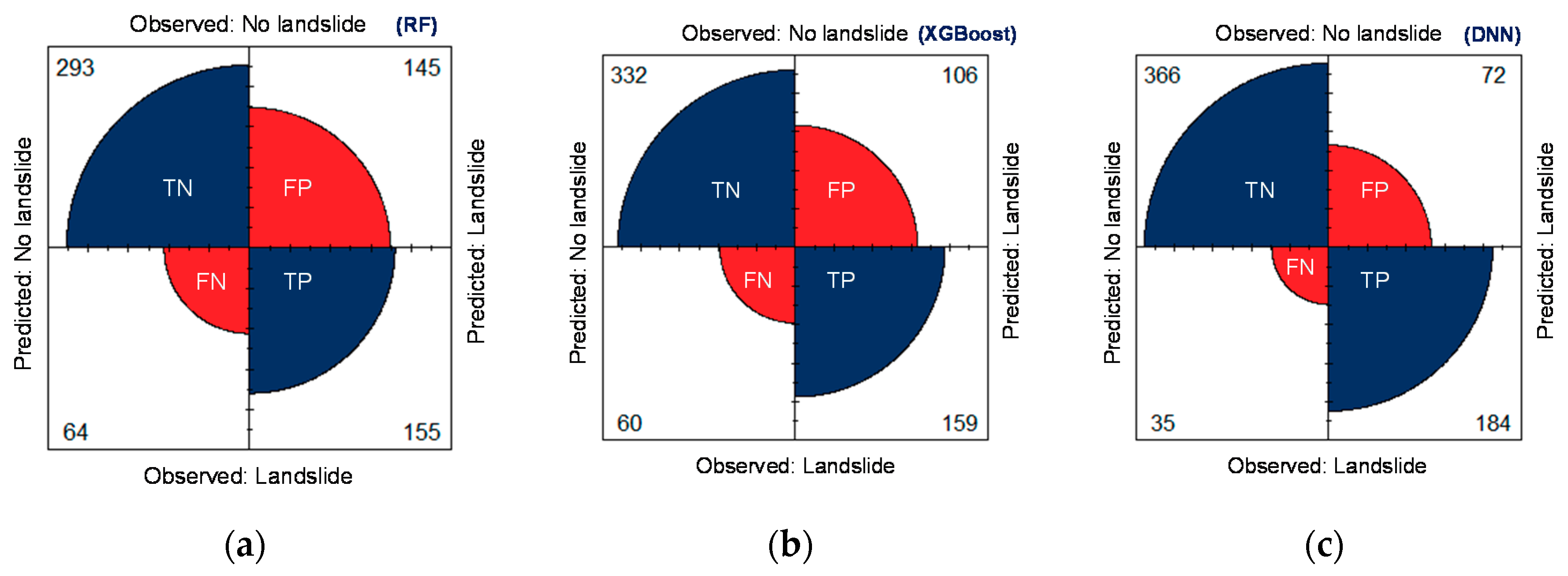
| Data Set | Model | TP | FP | FN | TN | Specificity (%) | Sensitivity (%) | ACC (%) |
|---|---|---|---|---|---|---|---|---|
| Testing | RF | 155 | 145 | 64 | 293 | 66.89 | 70.77 | 68.19 |
| XGBoost | 159 | 106 | 60 | 332 | 75.79 | 72.6 | 74.73 | |
| DNN | 184 | 72 | 35 | 366 | 83.56 | 84.01 | 83.71 |
© 2020 by the authors. Licensee MDPI, Basel, Switzerland. This article is an open access article distributed under the terms and conditions of the Creative Commons Attribution (CC BY) license (http://creativecommons.org/licenses/by/4.0/).
Share and Cite
Pradhan, A.M.S.; Kim, Y.-T. Rainfall-Induced Shallow Landslide Susceptibility Mapping at Two Adjacent Catchments Using Advanced Machine Learning Algorithms. ISPRS Int. J. Geo-Inf. 2020, 9, 569. https://0-doi-org.brum.beds.ac.uk/10.3390/ijgi9100569
Pradhan AMS, Kim Y-T. Rainfall-Induced Shallow Landslide Susceptibility Mapping at Two Adjacent Catchments Using Advanced Machine Learning Algorithms. ISPRS International Journal of Geo-Information. 2020; 9(10):569. https://0-doi-org.brum.beds.ac.uk/10.3390/ijgi9100569
Chicago/Turabian StylePradhan, Ananta Man Singh, and Yun-Tae Kim. 2020. "Rainfall-Induced Shallow Landslide Susceptibility Mapping at Two Adjacent Catchments Using Advanced Machine Learning Algorithms" ISPRS International Journal of Geo-Information 9, no. 10: 569. https://0-doi-org.brum.beds.ac.uk/10.3390/ijgi9100569