Improved Estimations of Nitrate and Sediment Concentrations Based on SWAT Simulations and Annual Updated Land Cover Products from a Deep Learning Classification Algorithm

Abstract

The agricultural sector and natural resources are heavily interdependent, comprising a coherent but complex system. The soil and water assessment tool (SWAT) is widely used in assessing these interdependencies for regional watershed management. However, long-term simulations of agricultural watersheds are considered as not realistic since they have often been performed assuming constant land use over time and are based on the coarse resolution of the existing global or national data. This work presents the first insights of the synergy among SWAT model and deep learning classification algorithms to provide annually updated and realistic model’s parameterization and simulations. The proposed hybrid modelling approach couples the physical process SWAT model with the versatility of Earth observation data-driven non-linear deep learning algorithms for land use classification (Overall Accuracy (OA) = 79.58% and Kappa = 0.79), giving a strong advantage to decision makers for efficient management planning. A validation case at an agricultural watershed located in Northern Greece is provided to demonstrate their synergistic use to estimate nitrate and sediment concentrations that load in Zazari Lake. The SWAT model has been implemented under two different simulations; one with the use of a static coarse land use map and the other with the use of the annual updated land use maps for three consecutive years (2017–2019). The results indicate that the land use changes affect the final estimations resulting to an enhanced prediction performance of 1% and 2% for sediment and nitrate, respectively, when the annual land use maps are incorporated into SWAT simulations. In this context, a hybrid approach could further contribute to addressing challenges and support a data-centric scheme for informed decision making with regard to environmental and agricultural issues on the river basin scale.

1. Introduction

A deeper understanding of the agricultural sector is needed to provide an informed and transparent framework required to meet increasing resource demands and pressures, without compromising sustainability. In this regard, an integrated management of the ecosystems is critical to address the priorities laid out by global policies and, achieve land degradation neutrality and resource efficient regions. In this regard, the importance of undertaking quantitative assessments and corresponding reporting of degraded lands across various scales to halt and reverse current trend in degradation has been recognized and prioritized [1].

To ensure tangible results in achieving land degradation neutrality, informed decisions based on comprehensive analyses are required, integrated at scale sufficient to support both sustainable land management and planning [2]. Thus, a data-driven approach to environmental protection promises to make it easier to spot problems, highlight policy failures and identify best practices.

In this context, the soil and water assessment tool (SWAT), a large-scale hydrologic and water quality physically-based model has proven its capabilities as an essential tool in examination of agronomic and environmental impacts of various management practices and relevant terrestrial resources planning [3]. Evidently, a number of research studies have been conducted in the area of modelling water and nutrient fluxes, ranging from few hundreds km² [4] to regional [5,6] scales. In addition, numerous studies have used scenario-based methods to quantify the impacts of land use on hydrological components with the SWAT model [7,8], while several studies examine how the land use change affects the concentrations of nitrate [9] and sediment [10,11] in the catchment area.

Overall, in the case of SWAT simulations reliable and accurate data and information are required. Spectral, temporal and spatial features derived from Earth observation (EO) systems can facilitate the systematic monitoring of the Earth’s land surface. With the support of high spatial resolution EO data (10 m), researchers and policy makers have the means to detect the changes and disturbances of land use/land cover (LULC) classes based on a time-series of satellite imagery data to provide high resolution and updated LULC maps and to improve physically process modelling. It is noteworthy that the importance of monitoring LULC for evaluating compliance with policies in force has been recognized and prioritized with the use of spaceborne data at global level [12]. Recently, the arrival of the era of deep learning (DL) for EO-based land cover mapping generated dual view [13] and multi-source [14] DL architectures that have attained significant improvements to reach the desired spatiotemporal representativeness and reliability for LC mapping. This can open a new era for operational terrestrial monitoring without the need for additional implemented training and validation data collection procedures.

Despite the usefulness of annual LC maps that can be derived from remote sensing time series, most of the strategies proposed for SWAT analysis, apply static coarse cover maps from relevant data archives, thus ignoring any spatiotemporal land change processes that may be discovered by the EO derived LULC maps. To our knowledge, there are only a few studies that used remote sensing LULC maps in combination with the SWAT model [15,16,17,18]. Thus, the exploitation of sophisticated non-linear models can be a game changer in classifying remote sensing time series data and generating spatial explicit indicators and incorporating them into physical based models.

Building upon the existing SWAT physical process model and non-linear classification algorithms, the current study will strive to deliver preliminary insights of the synergistic use of annual updates on land cover derived from EO imagery data and possible spatio-temproral based simulations to monitor and predict nitrate and sediment concentrations that load to a small surface water body in Northern Greece. The results of this study demonstrate a paradigm-shift from standard static water and land resource quantification toward generating more dynamic, on-demand, natural resource management strategies through the integration of state of the art DL algorithms to handle large volume of satellite imagery. The novel element of the proposed hybrid approach is that it paves the way for the assessment of the environmental impact of the agricultural sector, drawing knowledge from heterogeneous data of various scales for measuring the environmental performance of current and upcoming policies.

2. Materials and Methods

The proposed hybrid approach couples the physical process SWAT model with the versatility of EO-data driven non-linear classification algorithms for land use classification. In this regard, we based our analyses on multitude of information as inputs, such as multispectral spaceborne open EO data (Copernicus), the aerial imagery digital elevation model (DEM) and other spatial explicit indicators from relevant data archives. The overall data processing and analysis workflow is illustrated in Figure 1, while detailed descriptions of the different steps are provided in the sections below.

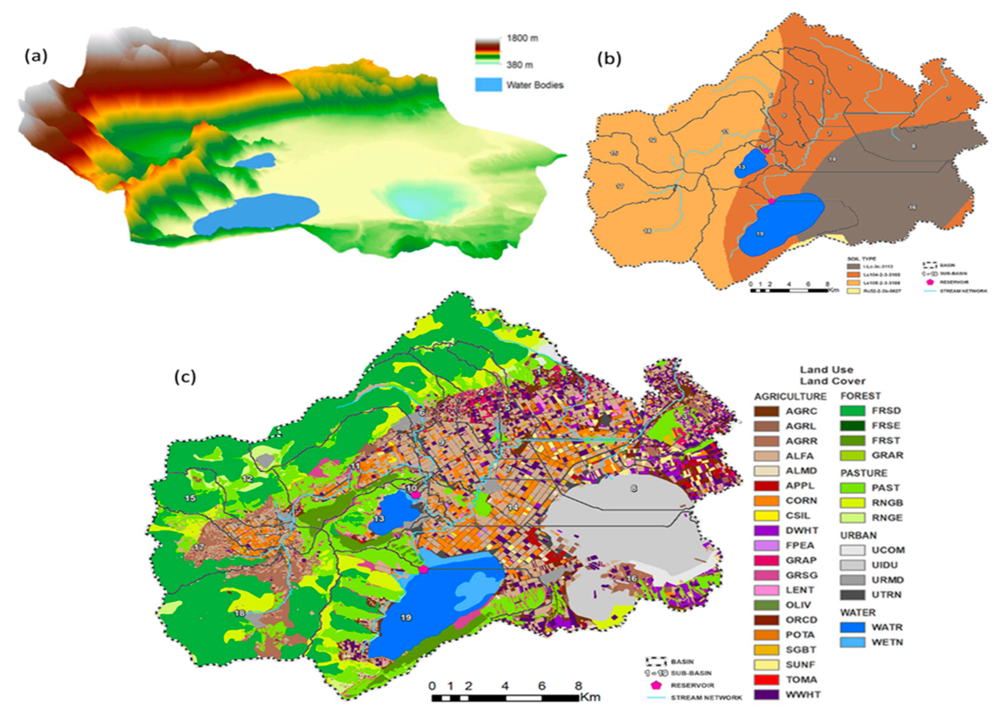
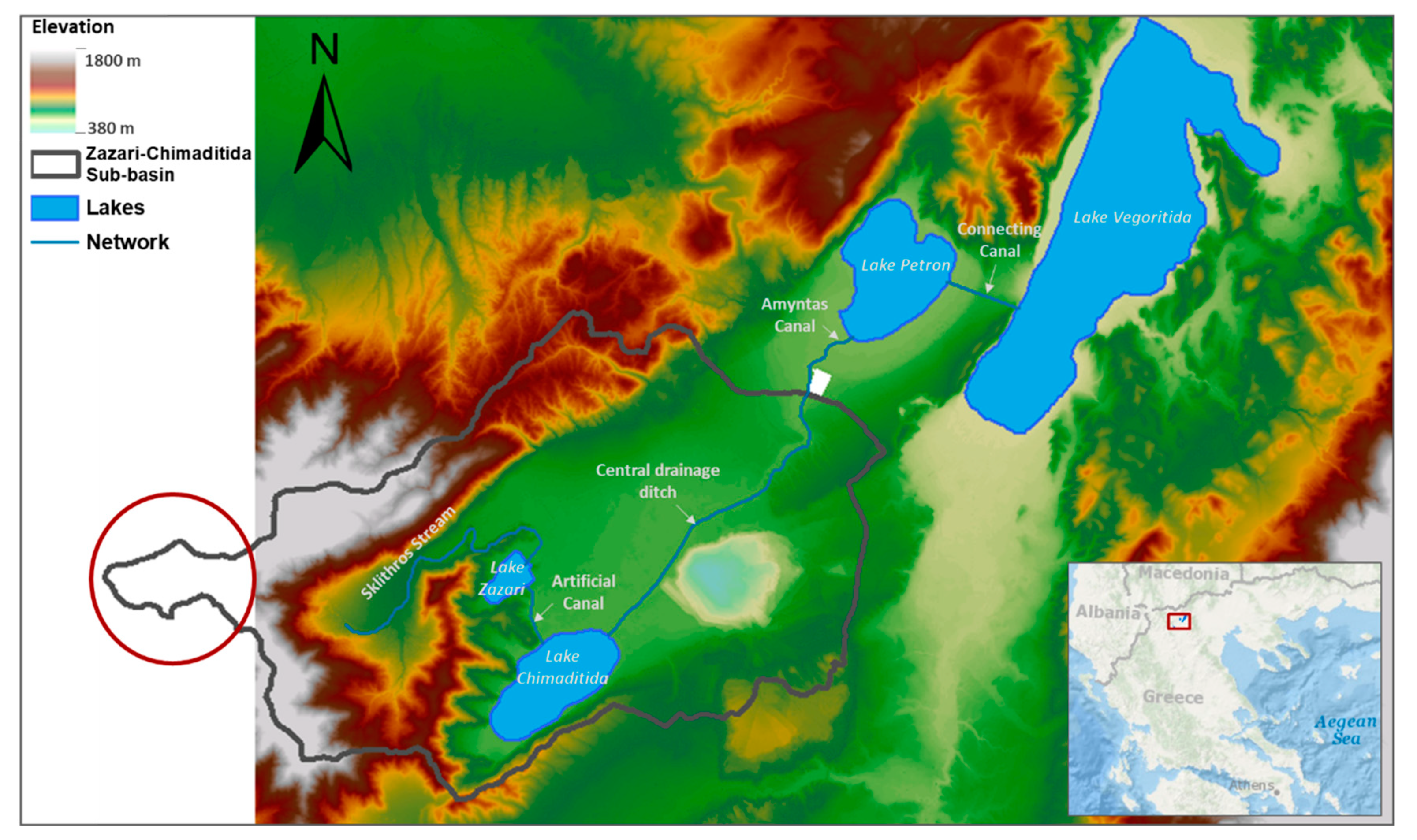
2.1. Description of the Study Area

The study area includes the hydrologic basin of two Lakes in Greece, Zazari, and Chimaditida, with a special focus to Lake Zazari in order to validate the nitrate and sediment concentrations. The Zazari-Chimaditida river sub-basin is located at the eastern part of the Vegoritida watershed and occupies over 216 km², and it is considered as one of the most important wetlands in Greek territory (Figure 2). The morphology of the region of interest is characterized by the presence of two sections, a mountainous area (19.05%) with intense relief and large slopes and a flat area (80.95%) with smooth slopes around the two lakes (Zazari and Chimaditida) and in the valleys. The climate of the study area can be classified by Köppen as hot-summer Mediterranean climate (Csa) [19]. The elevation of the river catchment ranges from 384 to 1796m. Due to its elevation (+600 m) and its long distance from the sea, it presents climatic characteristics different from those of the Greek Mediterranean type. Moreover, the lack of protective mountain areas from the North contributes to the formation of a continental climate. Lake Zazari (average depth of 4.6 m) has a natural flow towards Lake Chimaditida, with which it is connected. Considering that the geological formation of Lake Zazari was formed by large geological settlements, it is considered as tectonic. It is noteworthy that the main water entrance to the Zazari Lake is from the Sklithros stream, which make it also the main source of pollution for the lake. In the summer months the Sklithros stream usually has zero flow, but when the stream has water it is Zazari’s main water supplier. Zazari belongs to alpine-type lakes it is hot monomimetic with high nitrogen content and increasing eutrophication as well as occurrence of microcystins [20].

2.2. Data Collection and Analysis

The overall proposed hybrid approach requires in situ meteorological variables, stream flow input information and spatially explicit data. Below we briefly present the main data sources.

2.2.1. In Situ Information Procurement

The climatic data were derived from a hydro meteorological station located within our region of interest (21.678881, 40.690079). The hydro meteorological data were obtained from the region of Western Macedonia, where the relevant data records of local stations in the catchment are kept updated. The climatic data refer to daily precipitation, temperature, relative humidity, wind speed and solar radiation for the period from 2006 to 2019. During summer maximum temperatures are recorded in July-August, while during winter minimum values in January. The driest month rains less than 30mm, while during the wettest winter, it is about three times more. The wind speed is of a light breeze, and relative humidity and solar radiation ranged at relatively moderate-to-high levels. A brief overview of the climatic observations is presented in

Table 1. Overview of the qualitative and quantitative information regarding the meteorological observations.

Meteorological Data (2006–2019)
Temperature °C		Rainfall mm			Other
Max	Min	Max	Mean Annual	Min	Driest Month	Wettest Month	Wind speed	Relative Humidity	Solar Radiation
41.12	−14.6	857	615.3	374	30 mm	90 mm	Light breeze	Moderate to high	Moderate to high

.

Furthermore, for calibration and validation purposes of the model, monthly observed stream flow data from the years 2011 to 2014 were collected at the inlet of Zazari Lake. The stream flow data were obtained by Aristotle University of Thessaloniki, where historical archives of the relevant data records are kept. In addition, within the framework of the AquaNEX project one telemetric station was installed at the inlet of the Zazari Lake, giving monthly nitrate values and data of observed sediment for the second semester (July–December) of 2019.

2.2.2. Spatially Explicit Data

In this study, it is noteworthy that, the DEM used could not cover the entire Zazari-Chimaditida river sub-basin area (Figure 2, red circle). Hence, a small area (approximately 7 km²) in the western part was excluded from the rest of the analysis, without significantly affecting the final results and the stability of the model. For stream delineation purposes, we obtained a two-meter resolution DEM from a previous airborne campaign in 2018, which has been used for delineating the sub-river basin watershed and stream network (Figure 3a). Based on these values, the slope map was reclassified into four slopes (0–2.6%, 2.6–10.4%, 10.4–20.1% and more than 20.1%). Considering the soil data, we utilized a grid soil map from the Food and Agriculture Organization of the United Nations digital soil data hub. The Cambisols, Lithosols, Luvisols and Regosols are the dominant soils in the area (Figure 3b).

In addition to the topographic data, other data sources were needed as well, such as the land cover. In this study a dataset of geo-referenced polygons of land parcels and information on the type of land cover according with their area was utilized. This product is a combination of (i) the Greek Integrated Administration and Control System of 2017; (ii) in situ recordings for ground truth validation; and (iii) photo interpretation of very high-resolution spaceborne images. Note that the in situ data collection is not through the use of volunteer efforts but instead by a group of highly trained experts involved in the data collection, during the field campaigns of the AquaNEX research project. Water and built-up surfaces are derived from the national data archive. Prior to merging these data, they were checked for consistency and if needed, re-warped to the universal transverse mercator (UTM) coordinate system, resampled to 10 m and retiled into the Sentinel-2 tiling grid. Then, this information was converted into raster format. This land cover product hereinafter called as the combined reference dataset (Figure 3c). The final reference data includes 2,158,324 pixels distributed over 33 classes (see Appendix A). Based on this, the LC was categorized into agricultural land (24.26%), forest (68.50%), orchard (0.23%), grassland (3.15%), water (1.97%), wetland (0.42%), urban land (1.46%), and barren land (0.01%).

Then, the decision was made to follow an object-partitioning approach to guarantee that calibration and independent validation pixels were located in different land objects (e.g., neighborhood of pixels). A set of 70,000 random points generated within the boundary shapefile of the entire river basin and utilizing the Voronoi polygons a layer of smaller polygons was generated. Then, the labelled raster (33 classes) was polygonized and intersected with the created sub-polygons layer to ensure that all areas of the polygonized labelled data were contained within one of the created sub-polygons. The generated objects were separated into a randomly selected train (90%) and a test set (10%) with the total number of pixels varying between classes.

One main improvement in the proposed approach is the utilization of spaceborne EO imagery data to provide annual updates in the land cover map at 10m spatial resolution (see Section 2.3). In the current work, only visible (B2, B3, B4), near-infrared (B5-B8 and B8a) and short wave infrared (B11, B12) bands were used for both Sentinel-2A and Sentinel-2B Level-2A. To mitigate the limitation that arises due to cloud cover, we applied a selection criterion to cloud percentage (<10%) when generating our nearly cloud-free time series. Sitokonstantinou et al. [21] indicated that the utilization of dense satellite time series data regardless of the cloud coverage offered only a marginal increase in accuracy for a disproportionally larger cost in processing time. Consequently, it was decided to select satellite acquisitions that covers critical phenological stages of the targeted agricultural classes. In this context, the available Sentinel-2 images for the study area were downloaded from the Copernicus Open Access Hub. Figure 4 illustrates the selected Sentinel-2 acquisitions for 2017–2019 period, along with the phenology stages of agricultural classes (aquatic and urban classes are not presented). In the last step of pre-processing the bands at 20 m resolution (B5-B7, B8a, B11 and B12) were resampled at 10 m using a bicubic interpolation. These multispectral bands from the selected satellite observations constituted the classification features and were extracted for further processing.

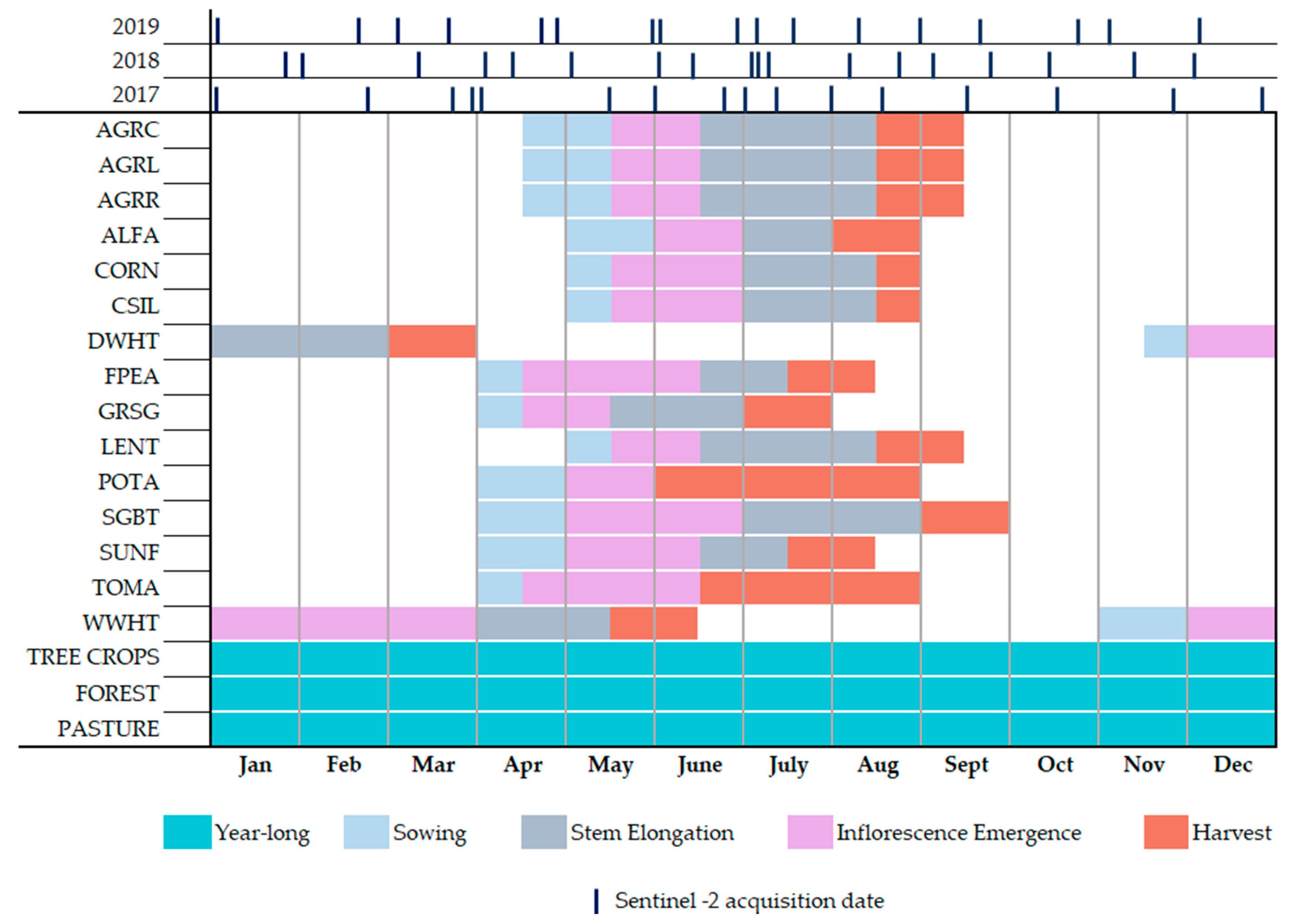
2.3. Generation of Annual Land Cover Dynamic Maps

Previous works indicated great potential in the utilization of non-linear deep learning methods for land cover classification with time series data from EO multispectral systems [13,14,22]. The Sentinel-2 time series together with the combined reference dataset for 2017 were inputs for the supervised classification algorithm in this study. Crop type prediction models were built based on a convolutional neural network (CNN) that has been utilized in a recent study [13].

The proposed network is arranged in a series of four different types of layers, namely: (i) the input layers, where the remotely sensed time series accounted for constituting the model’s input channel (ii) the two-dimension convolutional layers, which filters a given input and extracts information from specific spectral regions by carrying out the convolution operation; (iii) the flattening layer, which converts the multi-dimensional filters into a single continuous vector; and (iv) the dense layer, which connects all outputs of the previous layer to all inputs of the forthcoming layer. In the proposed architecture, we can notice that the first convolution has a kernel of 3 × 3 and it generates 256 feature maps, while the subsequent one generates 512 feature maps and still applies a kernel of 3 × 3. The last convolutional layer utilizes a kernel size of 1 × 1 and is mainly devoted to increasing the final number of extracted features to 1024. All the convolutions are followed by batch normalization, dropout (0.4), as well as a rectifier linear unit (ReLU) activation function (α = 0.01).

For the quantitative evaluation, the land cover map generated was assessed using an independent validation dataset which includes 140,689 sampling pixels (6.52% of the total surface) across the 33 classes. The classification performance for 2017 was obtained using the overall accuracy and the kappa coefficient.

2.4. The SWAT Model

The SWAT model was firstly proposed by Arnold, et al. [23]. The SWAT model is developed to predict the impact of land management practices on water, nutrients, sediments and agricultural yields in large complex watersheds with varying soils, land use and management conditions over a long period of time. It can also be used to predict water and soil loss in agriculturally dominant small watersheds [24]. The model is a physically based, offers flexibility and efficiency in the computational process and uses readily available data, making it perfectly suitable for the simulation of our study area. In general, the watershed in SWAT is divided into multiple sub-watersheds, connected by a stream network, which are then subdivided into hydrological response units (HRUs) consisting of unique combinations of land cover and soils in each sub basin.

The amount of nitrate moved with the water is calculated by multiplying the nitrate concentration in the mobile water by the volume of water moving in each pathway. Sediment yield are estimated for each HRU with the modified universal soil loss equation (MUSLE) [25].

2.4.1. SWAT Model Set Up

In the current study, the SWAT model was set-up to run on monthly bases considering the first four years (2009–2012) of data for the warm up period. For this study, the minimum threshold area of 433.5 ha was used to divide the catchment into 19 sub-basins. After the calculation of the sub basin parameters, two reservoirs (Lakes Zazari and Chimaditida) were located in the stream network. The land use baseline map that was used for the initial model set up was the combined reference dataset (Section 2.2.2). In addition multiple HRUs with 5% land use, 10% soil and 10% slope thresholds were utilized and the overlay of the sub basins, land use, soil and slope generated 284 HRUs.

2.4.2. Sensitivity Analysis, Calibration and Validation

In this study calibration and validation of the SWAT model were carried out using a four year period (2011–2014) based on monthly observed stream flow data which were collected at the inlet of Lake Zazari. The dataset was divided into calibration 2011–2013 and validation 2014 periods. Calibration and validation were carried out in SWAT calibration and uncertainty procedures (SWAT-CUP) 2012 using the sequential uncertainty fitting (SUFI-2) analysis algorithm, as it has been implemented in previous studies [26].

The first step in the calibration and validation process in SWAT is the determination of the most sensitive parameters for a given watershed. Sensitivity analysis (SA) is helpful to identify and rank the parameters that have significant impact on specific model outputs of interest [27]. In this study the results of the global SA performed in SWAT CUP using the SUFI-2 algorithm [28]. The analysis was carried out on a daily time step in order to accurately preserve the hydrologic characteristics of the watershed. The number of simulations used was 1000, which is adequate to obtain accurate results for a global SA [26]. SA determined the most sensitive parameters in this study area, as defined in

Table 2. SWAT sensitivity analysis and calibration results in the river sub-basin of Lakes Zazari and Chimaditida.

Parameter SWAT Code	Description	Statistical Indices		Range		Fitted Value
		t-Stat	p-Value	Min	Max
CN2	Soil conservation service (SCS) runoff curve number	−2.9339	0.0324	35	98	64
ALPHA_BF	Base flow recession constant	−0.5717	0.5922	0	1	1
GWQMN	Threshold depth for return flow of water in the shallow aquifer	3.5081	0.0171	0	5000	1150
GW_DELAY	Groundwater delay in days	4.3518	0.0073	0	500	14
GW_REVAP	Groundwater revap coefficient	1.0249	0.3633	0.02	0.2	0.2

. The t-statistic gives a measure of the sensitivity of the parameter, where those larger in absolute values are more sensitive. The p-values show the significance of the sensitivity, where p-values closer to zero are more significant. In this context, they have been used to provide a measure and significance of sensitivity.

2.4.3. Validation of the Results

The accuracy of the proposed approach was finally evaluated by examining the regression correlation coefficient (R²), the Nash-Sutcliffe model efficiency coefficient (NSE), percent bias (PBIAS), root mean square error (RMSE)-observations and the standard deviation ratio (RSR), which are calculated using Equations (1)–(4).

$${\mathit{R}}^2=\frac{{\left[{\sum }_{i=1}^n(O_i-\overline{O}){\left(P_i-\overline{P}\right)}^{ }\right]}^2}{\left[{\sum }_{i=1}^n{\left(O_i-\overline{O}\right)}^2\right]\left[{\sum }_{i=1}^n{\left(P_i-\overline{P}\right)}^2\right]}$$

(1)

$$\mathit{N}\mathit{S}\mathit{E}=\frac{{\sum }_{i=1}^n{(O_i-\overline{O})}^2-{\left(P_i-\overline{P}\right)}^2}{{\sum }_{i=1}^n{(O_i-\overline{O})}^2}$$

(2)

$$\mathit{P}\mathit{B}\mathit{I}\mathit{A}\mathit{S}=\left[\frac{{\sum }_{i=1}^n\left(O_i-P_i\right)\ast 100}{{\sum }_{i=1}^n\left(O_i\right)}\right]$$

(3)

$$\mathit{R}\mathit{S}\mathit{R}=\frac{RMSE}{STDE{V}_{obs}}=\frac{\left[\sqrt{{\sum }_{i=1}^n{\left(O_i-P_i\right)}^2}\right]}{\left[\sqrt{{\sum }_{i=1}^n{\left(O_i-\overline{O}\right)}^2}\right]}$$

(4)

where: $P_i$ is the predicted values, $O_i$ is the observed values, $\overline{O}$ is the mean of the observed data, $\overline{P}$ is the mean of the predicted data, n is the total number of observations and $STDE{V}_{obs}$ is the standard deviation of the observed values. Moriasi et al. [29] suggest that NSE, PBIAS, and RSR are better quantitative statistics to evaluate model performance. They concluded that model simulation for monthly stream flow is satisfactory if 0.5 < NSE ≤ 0.65, 0.60 < RSR ≤ 0.70, and ±15 ≤ PBIAS < ±25. However, it is satisfactory for the sediment yield if ±30 ≤ PBIAS < ±55 with same values for NSE and RSR as reported for stream flow. Other studies have suggested that an R² value greater that 0.5 is considered acceptable [30,31].

2.4.4. Improvement in SWAT Predictions

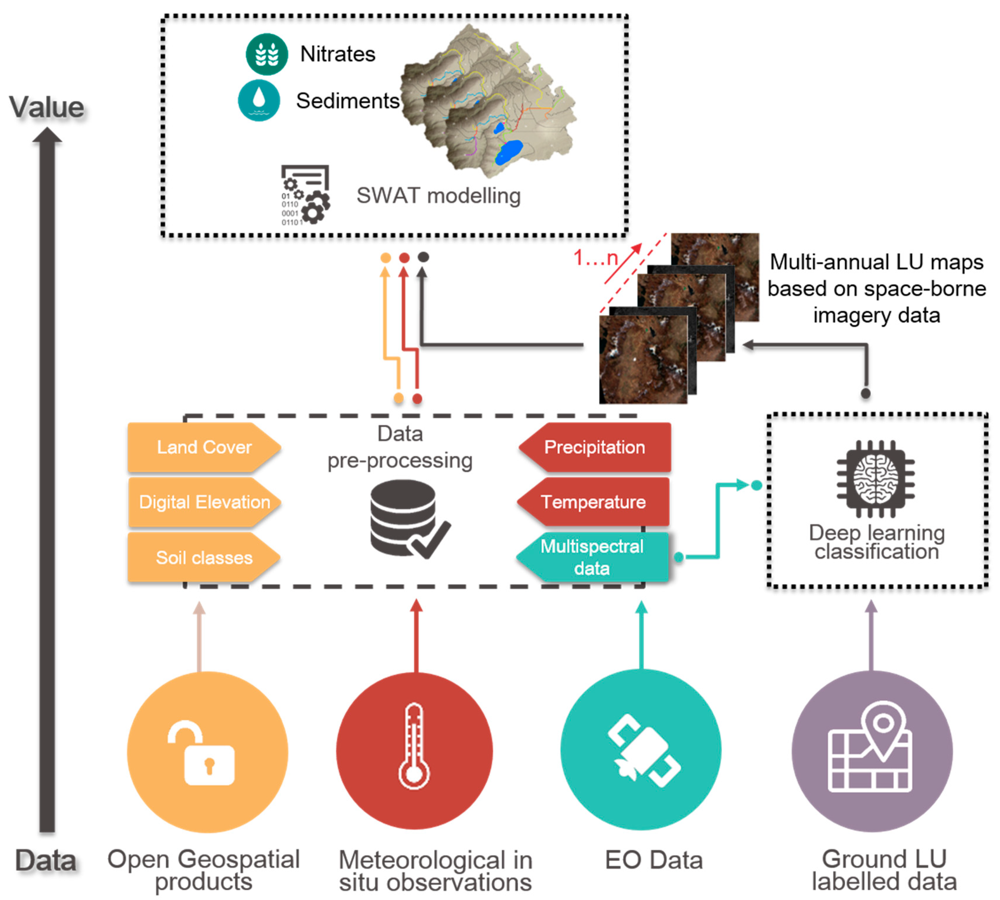
According to Hernandez et al. [32], to better understand any improvements due to temporally precise disturbance data, we explored the relationship between the number of HRUs and the total number of them:

Total HRUs = Initial HRUs₂₀₁₃ × Number of years with changes

(5)

and the relative improvement in the stream flow predictions defined by

Improvement = NSE or RSR_{using dynamic maps} − NSE or RSR_{using static maps}

(6)

Change is defined by the availability of a three or annual map.

2.5. Implementation

In this work, the Geographic Information System ArcGIS 10.5 was used for interfacing the SWAT hydrological model. The analysis of EO data was preformed on a local version of the Committee on Earth Observation Satellites data cube [33], making the whole processing routine more efficient and effective in terms of handling the EO data [34]. The features for classification corresponding to the classes were then extracted for further processing. The statistical and CNN classification analyses were performed utilizing the R software [35] with the keras package. The classification model was built on a workstation with a NVIDIA Quadro K4200 graphics processing unit.

3. Results and Discussion

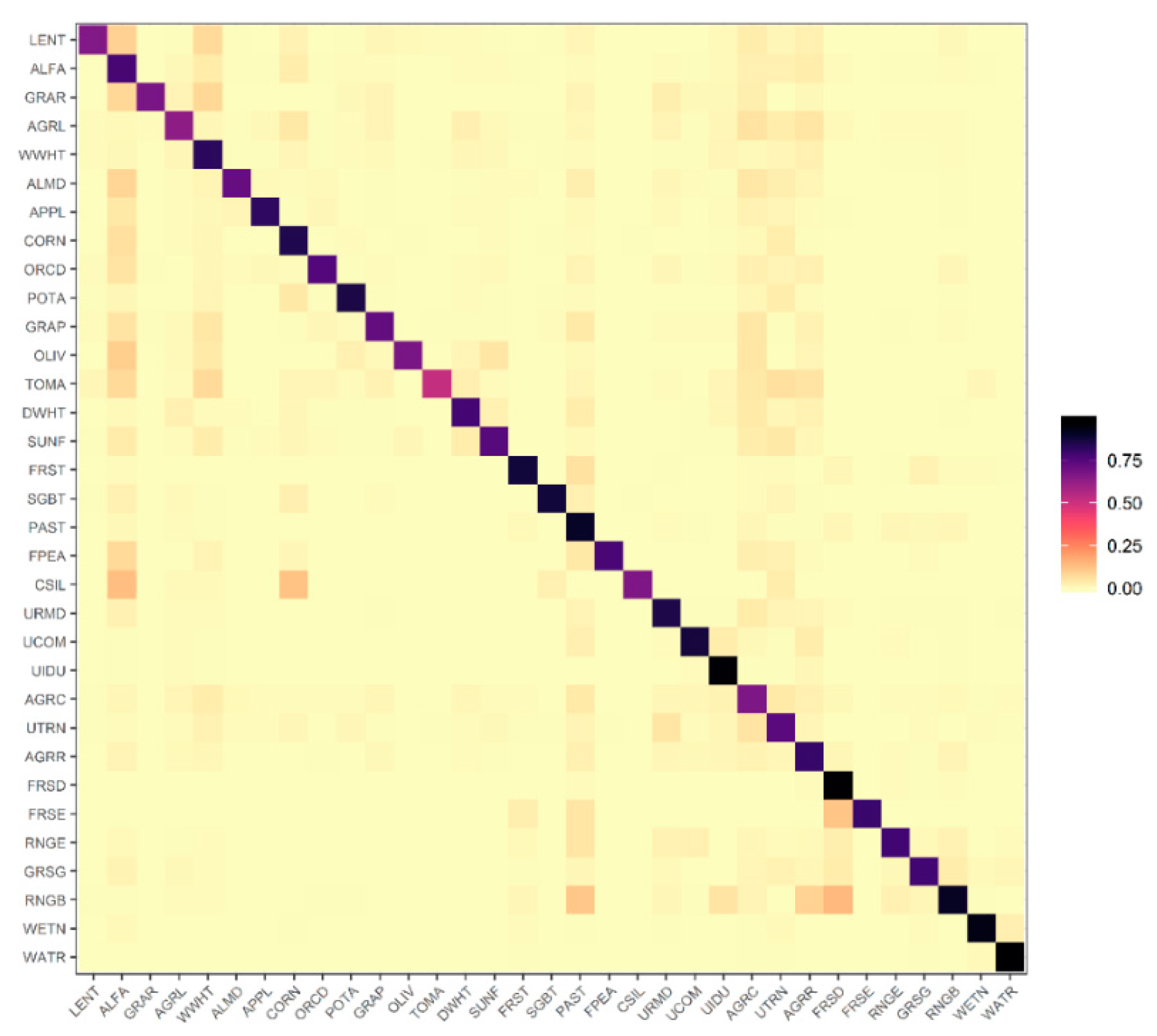
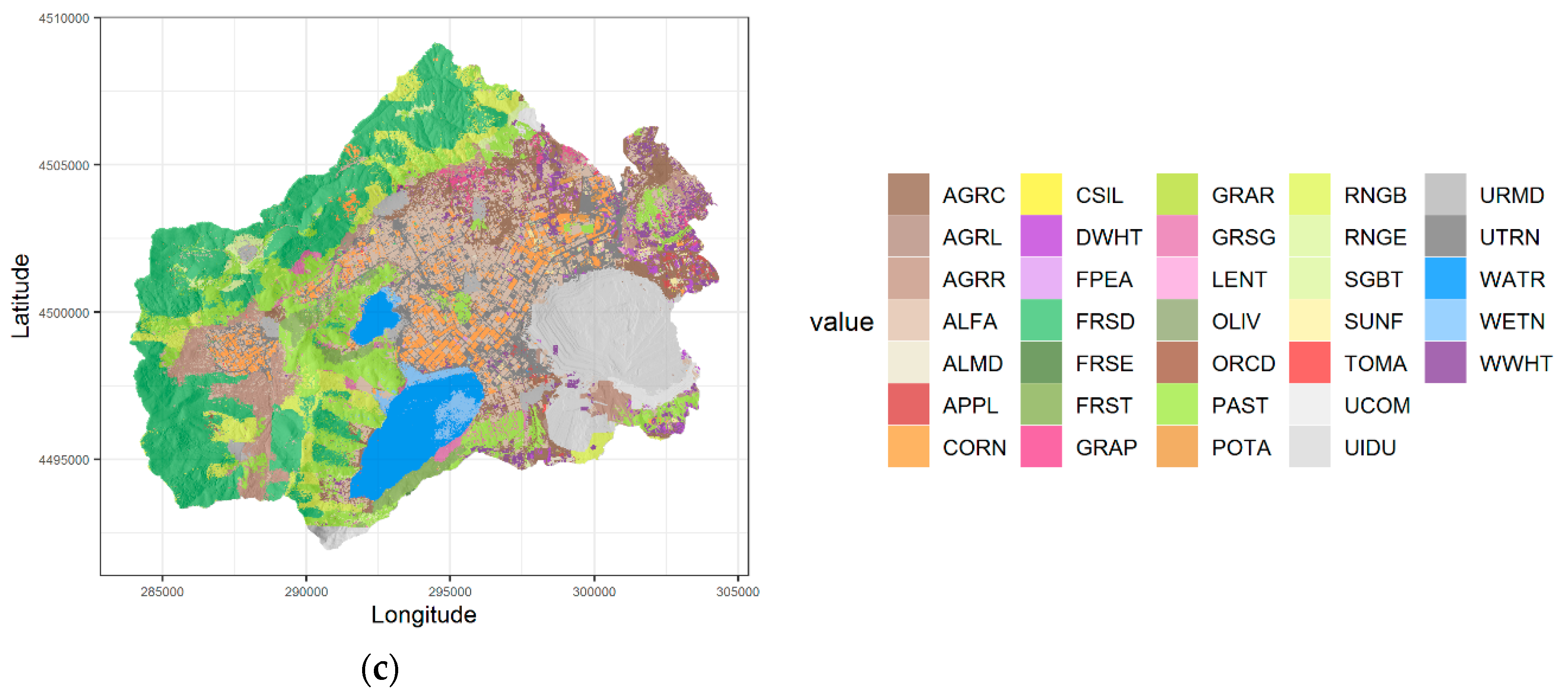
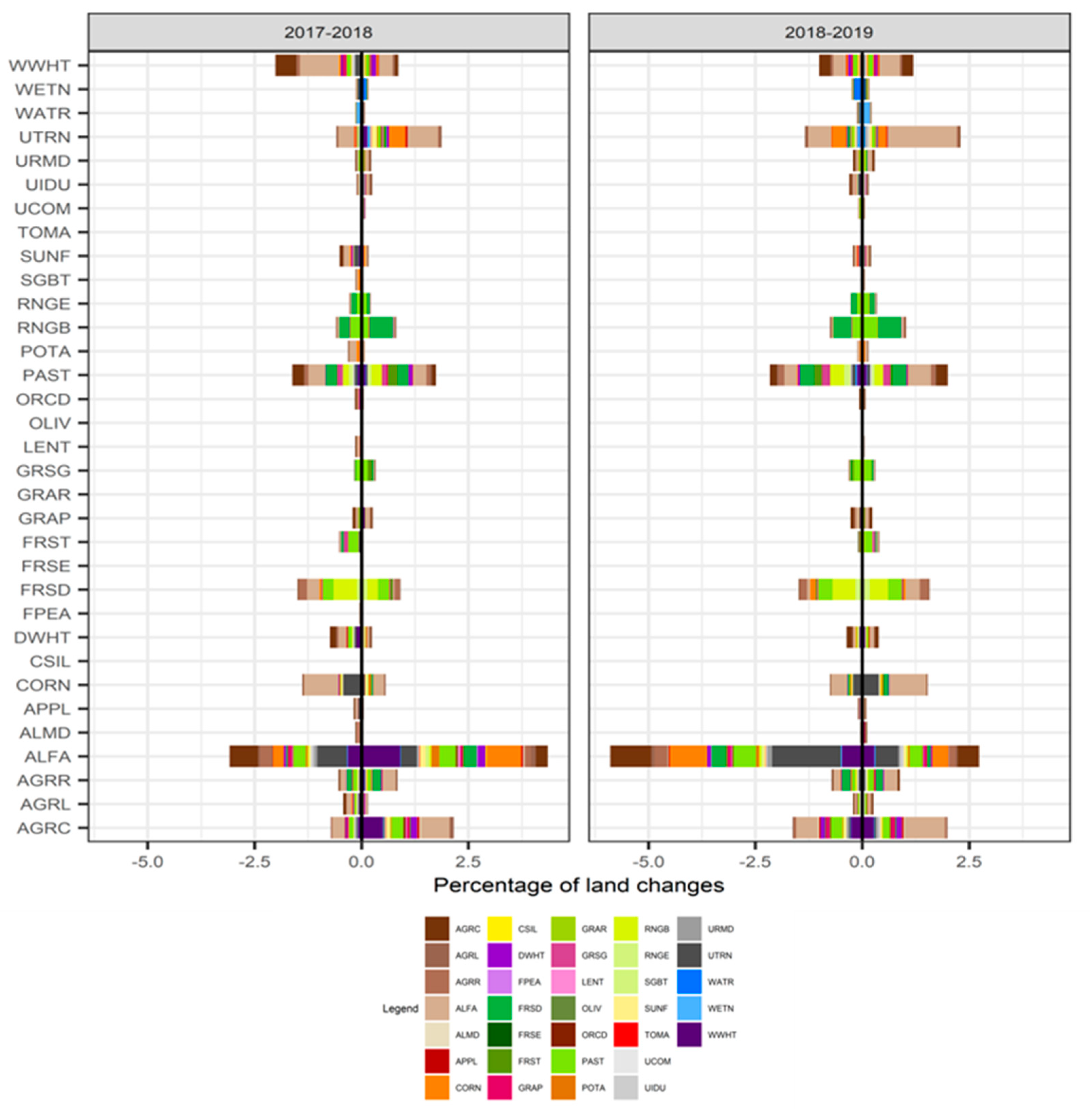
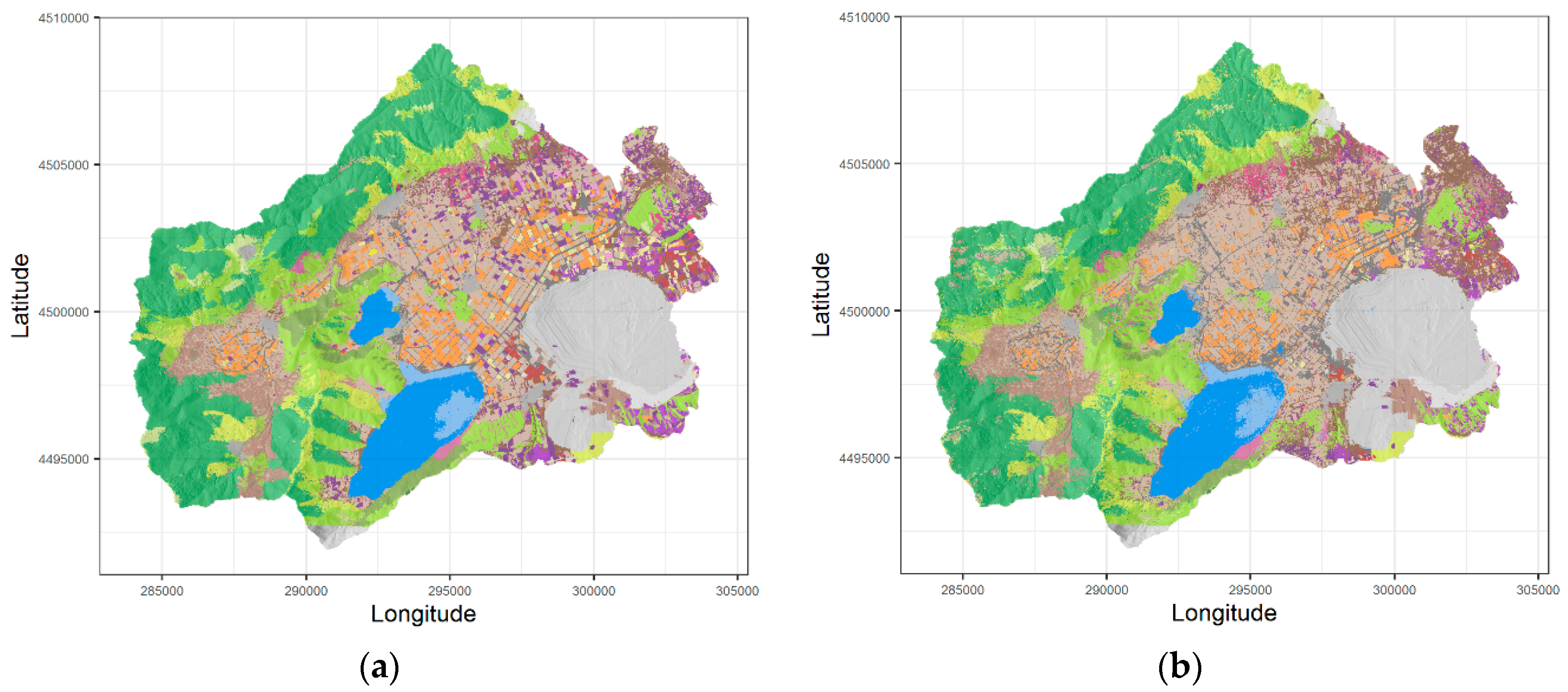
3.1. Remote Sensing Land Use and Land Cover Classification Results

We report here only a short summary of the classification results. Overall, the CNN achieved good classification results (Overall Accuracy (OA) = 79.58% and Kappa = 0.79) considering the ground truth data of 2017. In terms of class-specific accuracies wetlands, water bodies sugar-beet and tree crops (e.g., almonds, olives, apples etc.) are mapped with very high accuracies (>90%). Few classes such as grapes, wheat and the majority of urban land uses are moderate (>80%) while arable lands (alfalfa, agricultural land generic and close grown, as well as urban transportation) have lower-class accuracies (<65%). The visual results that support the previous section, are presented in terms of heat maps in Figure 5. This corresponds to the confusion matrix points of the CNN algorithm.

The most noticed difference between adjusted and predicted areas is produced for arable land classes. This can be explained by the underestimation of alfalfa due to its confusion with other relevant classes. It is noteworthy to mention that the small size in several parcels, as well as in a few classes (e.g., urban transportation) cannot be captured efficiently by Sentinel-2 resolution, and this may affect the classification performance. In addition, considering the pastures, rangelands and in general the open agricultural areas, we can observe moderate classification results due to their similar temporal patterns compared to other classes where they have distinctive temporal patterns within a growing season. In this context, classification should be performed taking into account the phenological cycles of each vegetation type investigated, and further research is required to increase the efficiency. The total agricultural areas remained stable across the three year period. In this regard, next to a discrete land cover layer for 2017, we generated the relevant products for 2018 and 2019 through the use of Sentinel-2 data and the developed classification algorithm (Figure 6).

When compared with the reference land cover dataset, the land cover maps of 2018 and 2019, respectively, show on a regional scale high dissimilarities, especially in the conversion of alfalfa crops into cereals (Figure 7).

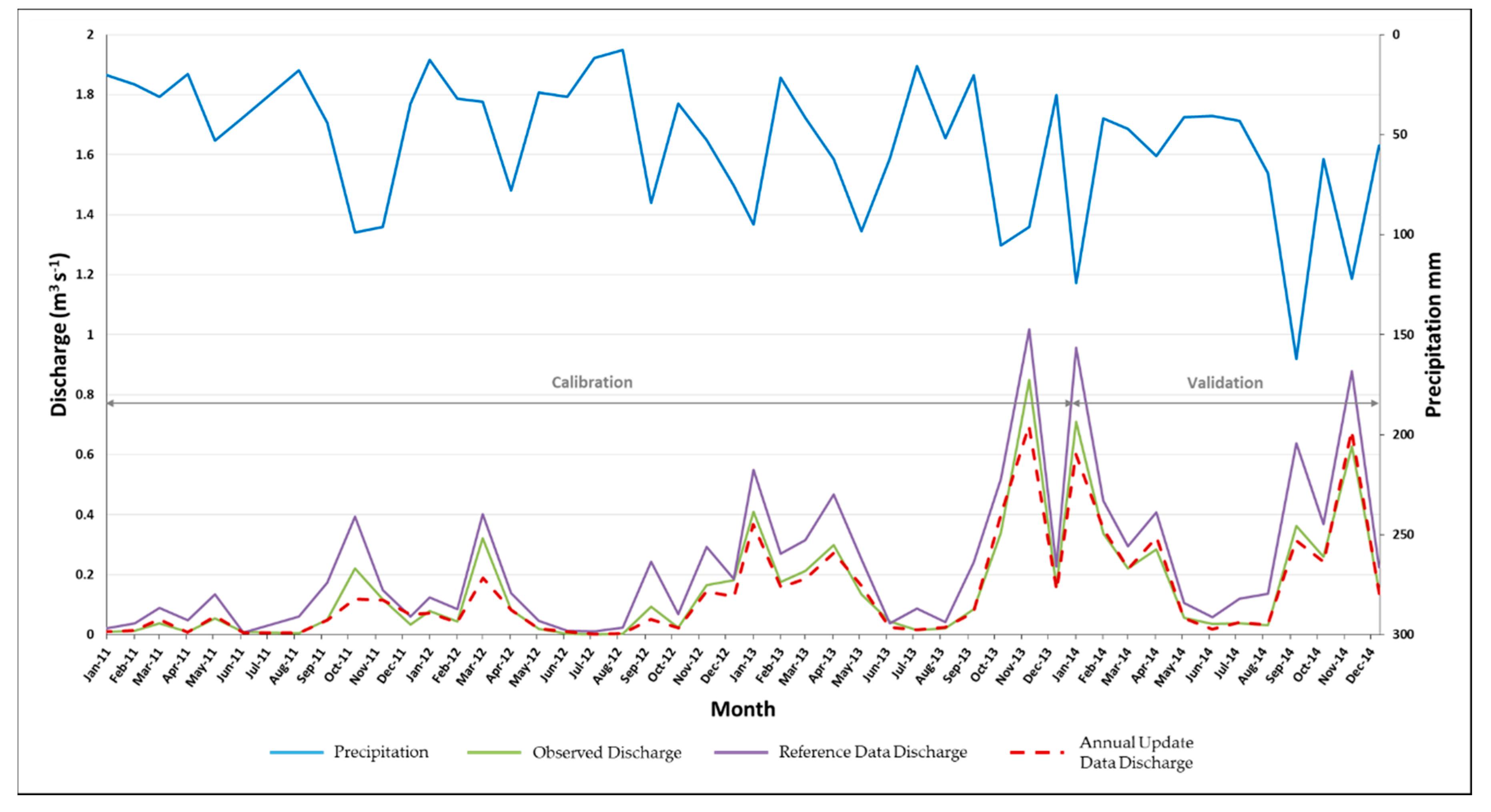
3.2. SWAT Calibration and Validation

As has already mentioned, the SWAT model was calibrated and validated at the inlet of the Lake Zazari where observed discharge load data were available. The performance evaluation of the SWAT model on the basis of monthly discharge is shown in

Table 3. Statistical metrics of calibration and validation phases.

Evaluation Statistics	Calibration		Validation
	Reference Data	Annual Update	Reference Data	Annual Update
R2	0.89	0.95	0.90	0.91
NSE	−0.56	0.31	−0.76	0.30
PBIAS	−58.65	14.2	−48.80	13.5
RSR	1.61	0.70	1.03	0.63

. Moreover, the observed and simulated monthly discharges for the calibration and validation periods are presented in Figure 8. The graphical representation and the statistical results show that the observed and simulated discharge closely match during the simulation period, except for some cases which were mostly underestimated due to high flow events like storms (Oct -11th, Mar -12th, Jul -13th, Jan -14th). Furthermore, the model performance was considered as sufficient due to the strong agreement between discharge and precipitation with only a set of small underestimations during the wet seasons.

The annual updates in LU maps generated by the Sentinel-2 data produced better performance estimates across the time series available for the watershed. Regarding the statistical evaluation the R² (0.95 for calibration and 0.91 for validation) values show very high consistency between the observed and simulated data results. For the PBIAS, we found 14.2 for calibration and 13.5 for validation which are acceptable results. Moreover, the values 0.7 for calibration and 0.63 for validation regarding the RSR showed a satisfactory consistency.

It is well stated that the rainfall -runoff and stream flow are the main driving forces behind the movement of sediment and nitrate through the watershed. Therefore, the appropriate calibration step of the SWAT model regarding the stream flow plays a vital role. It is noteworthy that the lack of a complete time series of nitrate and data of observed sediment did not allow the full calibration and validation for those parameters. At this point, it should be mentioned that a model calibrated, for example, for discharge, may not be adequate for prediction of sediment, or for application to another region, or for application to another time period [36]. However, a lot of research works has been done successfully in the past by calibrating the model with the discharge and simulating sediments [37] or implementing land use change scenarios [38]. In future research, the previous assumption will be considered by using the SWAT-CUP for calibration and validation purposes. The values of the observed and the model simulated stream flow were found to display a satisfactory statistical agreement. The results obtained from the model calibration and evaluation process (Table 3) for both reference and annual update data can be also explained due to the high spatial DEM resolution used in the simulation. Many studies report that DEM resolution is the most critical input for SWAT simulation [9,39,40,41], and, for this reason, in this study, a high spatial resolution of 2 × 2 DEM was used, giving a reliable and accurate stream network of the region of interest and therefore a very good overall watershed delineation.

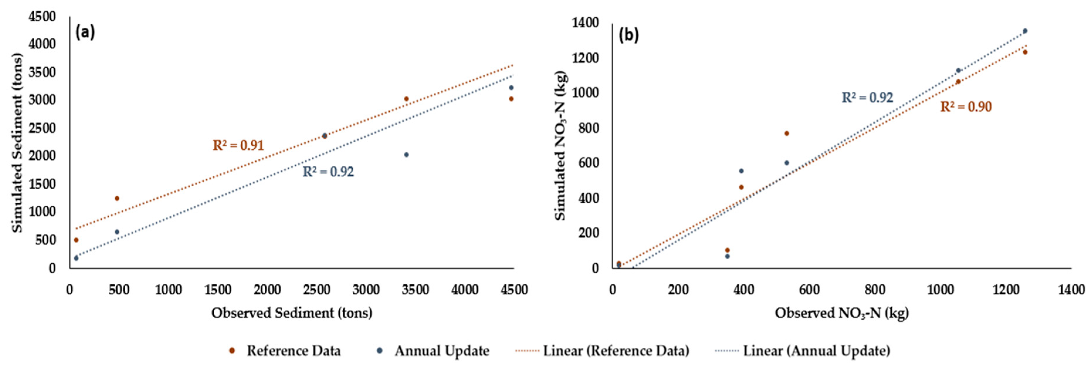
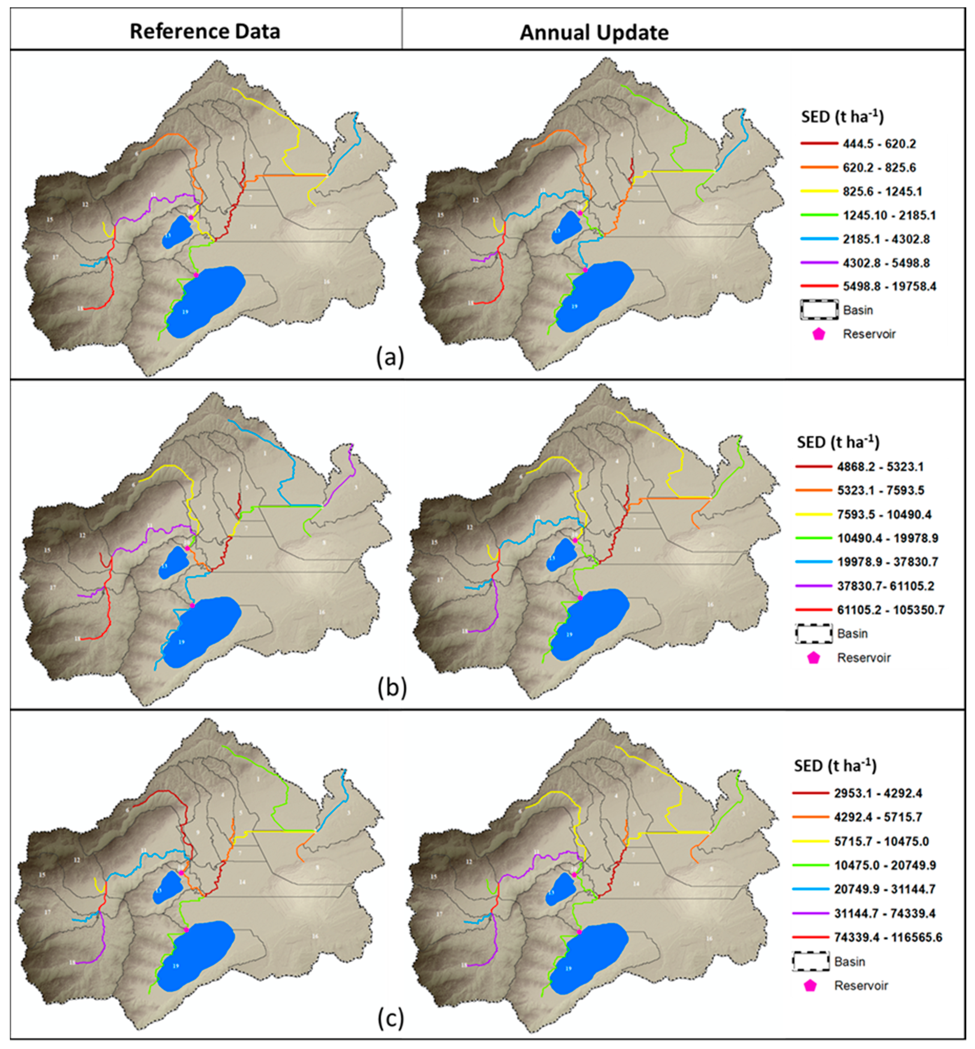
3.3. SWAT Model Simulation Results

Two different simulations were applied in the Zazari -Chimaditida river sub-basin area for assessing the effects of LULC change regarding the concentrations of sediment and nitrate that load in Zazari Lake. The first approach was based on a reference data digital map from 2013 to 2019 and the second one utilizing the annual updates of LU maps for 2017, 2018 and 2019. It should be mentioned that the other inputs such as DEM, soil, climate were kept the same in both simulations.

Considering the first approach, the results of the sum of average annual sediment and nitrate concentration that load to Zazari Lake are 102,597.84 tons and 7356.43 tons, respectively. The sum values regarding the simulation period 2013–2019 vary from 1415.51 to 24,194.68 tons for sediments and 384.07 to 1666.98 Kg for nitrate loads. The maximum values were obtained in 2015 and 2016 for sediments and nitrates, respectively, and the minimum in 2017 for both of the observed parameters. On the other hand, we evaluated the results as derived from the second approach. According to this simulation results, the sum average annual sediments and nitrate concentration that load to Zazari Lake are 106,459.26 tons and 7209.44 tons, respectively. The sum values regarding the total period vary from 1436.52 tons to 24,614.28 tons for sediments and 382.23 to 1674.56 Kg for nitrate loads. In addition, the maximum values were obtained in 2015 and 2016 for sediments and nitrates, respectively, and the minimum in 2017 for both of the observed parameters. In Figure 9, a comparison of the results considering the reference datasets and the annual updates in LU is illustrated for the years 2017, 2018 and 2019.

Comparing the values of the reference dataset with those of the average annual concentrations of sediment and nitrate that load in Zazari Lake, an overall increase of 3.76% in sediments and an overall decrease of 1.94% for nitrates were observed. The comparison results were realistic if we mention the LULC changes in the annual update EO-driven maps for the years 2017, 2018 and 2019.

Moreover, in both nitrates and sediments shown in Figure 10, the integration of annual LU maps in SWAT simulations, within a framework of a hybrid approach, can lead to results with enhanced prediction capabilities. Overall the annual updated LU products increase the R² by 1% and 2% for sediment and nitrates, respectively.

Soil nitrate leaching is greatly influenced by soil and climatic factors as well as agricultural management practices. This results in further deterioration of the surface water bodies as well as ground water reservoirs. For instance, corn crop is particularly demanding in water and sensitive to weed, thereby increasing the pressure on water bodies (intense agricultural practices). On the other hand, alfalfa crop has low demands on water and fertilization. Moreover, the forest areas in general have low water demands, and because of the strong tree root, they greatly impede the transport of sediments. In the light of the above, the inclusion of more hectares under alfalfa cultivation and pastures in conjunction with a significant decrease in corn cultivation areas (Figure 7) may explain the results in nitrates and sediments (Figure 10). Last but not least, the extreme values (max -min) of the concentrations of sediments and nitrates in the lake were found to agree in both simulations as far as the time of observation is concerned and as presented above. Sediments and nitrates are directly related to rainfall, and if one considers that the meteorological data entered in the SWAT model are the same for both simulations, then the extreme values regarding the year are considered reliable. Regarding the study area, the high annual rainfall values were observed in 2015 (814 mm) and 2016 (819 mm), and the minimum in the year 2017 (374 mm).

3.4. Source of the Improvement in Predictions

The introduction of annual update LU products derived from EO data in comparison with a reference static LU map also generated differences in the total number of HRUs that were available for SWAT to model changes from year to year. Considering the Equations (5) and (6) in conjunction with the simulations outputs of the SWAT model for the two approaches, we obtained 284 HRUs for the reference dataset in year 2013 and an increase of 14 HRUs when the updated LU maps (298 HRUs) were integrated. Based on Equation (5), the total HRUs were 894 for the second approach where we integrated LU products that were annually updated. In this context, a difference of 610 HRUs is observed between the total HRUs and the HRUs as recorded for the reference static map. Finally, obtaining the difference between the estimated NSE considering the reference static map and the annually update LU maps, the improvement in the NSE metric was calculated. The same formula was applied to evaluate the SWAT’s improvement in terms of RSR. In light of the above, the results showed a 0.87 and 0.01 higher performance for NSE and RSR, respectively. Our results are in agreement with those obtained in a previous study, where improved predictions in a stream flow were observed due to the utilization of updating land cover maps with EO -based forest change detection products [32].

4. Conclusions and Outlook

In this study, EO imagery data coupled with DL techniques were used in order to improve the performance of a physical process model (SWAT) and predict nitrate and sediments concentrations that load to Zazari Lake located in Northern Greece. In this case, the LULC change plays a vital role regarding sediment and nitrate concentration that can transfer via the watershed’s stream network into the area’s water bodies. The proposed hybrid approach is based on using detailed remote sensing annual maps derived from Sentinel-2, and with the use of a general DL framework to provide a reliable and accurate LULC classification (OA = 79.58% and Kappa = 0.79) of the entire river basin.

The simulations results indicate that the LULC changes affect the final estimations, resulting in an enhanced prediction performance of 1% and 2% for sediments and nitrates, respectively, when the annual land use maps are incorporated into physical -based process model simulations. In this context, a hybrid approach could further contribute to addressing challenges and support a data-centric schemes for informed decision making with regard to environmental and agricultural issues on the river basin scale. The study outcomes are relevant to improve decisions of policy makers, concerning agricultural and natural processes in general. It has strong potential to help the EU’s Common Agricultural Policy to meet its objectives concerning enhanced competitiveness of the agricultural sector and improved sustainability and effectiveness through reduced environmental impacts and utilization of natural resources in more sustainable and highly efficient manners. In future studies, we should prioritize an inferencing system that can be used on a large/regional scale and provide input as per the outcome of the direct payments scheme on specific sustainability performance indicators, such as land degradation, to allow for insightful decision making on a regional and/or national level.

References

1. Simpson, G.B.; Jewitt, G.P.W. The Development of the Water-Energy-Food Nexus as a Framework for Achieving Resource Security: A Review. Front. Environ. Sci. 2019, 7, 8. [Google Scholar] [CrossRef] [Green Version]
2. Giuliani, G.; Chatenoux, B.; Benvenuti, A.; Lacroix, P.; Santoro, M.; Mazzetti, P. Monitoring land degradation at national level using satellite Earth Observation time-series data to support SDG15 – exploring the potential of data cube. Big Earth Data 2020, 4, 3–22. [Google Scholar] [CrossRef] [Green Version]
3. Arnold, J.G.; Fohrer, N. SWAT2000: Current capabilities and research opportunities in applied watershed modelling. Hydrol. Process. 2005, 19, 563–572. [Google Scholar] [CrossRef]
4. Pandey, A.; Himanshu, S.K.; Mishra, S.K.; Singh, V.P. Physically based soil erosion and sediment yield models revisited. Catena 2016, 147, 595–620. [Google Scholar] [CrossRef]
5. Abbaspour, K.C.; Rouholahnejad, E.; Vaghefi, S.; Srinivasan, R.; Yang, H.; Kløve, B. A continental-scale hydrology and water quality model for Europe: Calibration and uncertainty of a high-resolution large-scale SWAT model. J. Hydrol. 2015, 524, 733–752. [Google Scholar] [CrossRef] [Green Version]
6. Garg, K.K.; Bharati, L.; Gaur, A.; George, B.; Acharya, S.; Jella, K.; Narasimhan, B. Spatial mapping of agricultural water productivity using the swat model in Upper Bhima catchment, India. Irrig. Drain. 2012, 61, 60–79. [Google Scholar] [CrossRef] [Green Version]
7. Cai, T.; Li, Q.; Yu, M.; Lu, G.; Cheng, L.; Wei, X. Investigation into the impacts of land-use change on sediment yield characteristics in the upper Huaihe River basin, China. Phys. Chem. Earth 2012, 53–54, 1–9. [Google Scholar] [CrossRef]
8. Memarian, H.; Balasundram, S.K.; Abbaspour, K.C.; Talib, J.B.; Boon Sung, C.T.; Sood, A.M. SWAT-based hydrological modelling of tropical land-use scenarios. Hydrol. Sci. J. 2014, 59, 1808–1829. [Google Scholar] [CrossRef]
9. Chaplot, V.; Saleh, A.; Jaynes, D.B. Effect of the accuracy of spatial rainfall information on the modeling of water, sediment, and NO3-N loads at the watershed level. J. Hydrol. 2005, 312, 223–234. [Google Scholar] [CrossRef]
10. Sorando, R.; Comín, F.A.; Jiménez, J.J.; Sánchez-Pérez, J.M.; Sauvage, S. Water resources and nitrate discharges in relation to agricultural land uses in an intensively irrigated watershed. Sci. Total Environ. 2019, 659, 1293–1306. [Google Scholar] [CrossRef] [PubMed]
11. Himanshu, S.K.; Pandey, A.; Yadav, B.; Gupta, A. Evaluation of best management practices for sediment and nutrient loss control using SWAT model. Soil Tillage Res. 2019, 192, 42–58. [Google Scholar] [CrossRef]
12. Buchhorn, M.; Lesiv, M.; Tsendbazar, N.-E.; Herold, M.; Bertels, L.; Smets, B. Copernicus Global Land Cover Layers—Collection 2. Remote Sens. 2020, 12, 1044. [Google Scholar] [CrossRef] [Green Version]
13. Interdonato, R.; Ienco, D.; Gaetano, R.; Ose, K. DuPLO: A DUal view Point deep Learning architecture for time series classificatiOn. ISPRS J. Photogramm. Remote Sens. 2019, 149, 91–104. [Google Scholar] [CrossRef] [Green Version]
14. Ienco, D.; Interdonato, R.; Gaetano, R.; Ho Tong Minh, D. Combining Sentinel-1 and Sentinel-2 Satellite Image Time Series for land cover mapping via a multi-source deep learning architecture. ISPRS J. Photogramm. Remote Sens. 2019, 158, 11–22. [Google Scholar] [CrossRef]
15. Fisher, J.R.B.; Acosta, E.A.; Dennedy-Frank, P.J.; Kroeger, T.; Boucher, T.M. Impact of satellite imagery spatial resolution on land use classification accuracy and modeled water quality. Remote Sens. Ecol. Conserv. 2018, 4, 137–149. [Google Scholar] [CrossRef]
16. Foteh, R.; Garg, V.; Nikam, B.R.; Khadatare, M.Y.; Aggarwal, S.P.; Kumar, A.S. Reservoir Sedimentation Assessment Through Remote Sensing and Hydrological Modelling. J. Indian Soc. Remote Sens. 2018, 46, 1893–1905. [Google Scholar] [CrossRef]
17. Azimi, S.; Dariane, A.B.; Modanesi, S.; Bauer-Marschallinger, B.; Bindlish, R.; Wagner, W.; Massari, C. Assimilation of Sentinel 1 and SMAP – based satellite soil moisture retrievals into SWAT hydrological model: The impact of satellite revisit time and product spatial resolution on flood simulations in small basins. J. Hydrol. 2020, 581, 124–367. [Google Scholar] [CrossRef]
18. Fallatah, O.A.; Ahmed, M.; Cardace, D.; Boving, T.; Akanda, A.S. Assessment of modern recharge to arid region aquifers using an integrated geophysical, geochemical, and remote sensing approach. J. Hydrol. 2019, 569, 600–611. [Google Scholar] [CrossRef]
19. Kottek, M.; Grieser, J.; Beck, C.; Rudolf, B.; Rubel, F. World Map of the Köppen-Geiger climate classification updated. Meteorol. Zeitschrift 2006, 15, 259–263. [Google Scholar] [CrossRef]
20. Christophoridis, C.; Zervou, S.-K.; Manolidi, K.; Katsiapi, M.; Moustaka-Gouni, M.; Kaloudis, T.; Triantis, T.M.; Hiskia, A. Occurrence and diversity of cyanotoxins in Greek lakes. Sci. Rep. 2018, 8, 17877. [Google Scholar] [CrossRef] [Green Version]
21. Sitokonstantinou, V.; Papoutsis, I.; Kontoes, C.; Lafarga Arnal, A.; Armesto Andrés, A.P.; Garraza Zurbano, J.A. Scalable Parcel-Based Crop Identification Scheme Using Sentinel-2 Data Time-Series for the Monitoring of the Common Agricultural Policy. Remote Sens. 2018, 10, 911. [Google Scholar] [CrossRef] [Green Version]
22. Wang, H.; Zhao, X.; Zhang, X.; Wu, D.; Du, X. Long Time Series Land Cover Classification in China from 1982 to 2015 Based on Bi-LSTM Deep Learning. Remote Sens. 2019, 11, 1639. [Google Scholar] [CrossRef] [Green Version]
23. Arnold, J.G.; Srinivasan, R.; Muttiah, R.S.; Williams, J.R. Large area hydrologic modeling and assessment part I: Model development. J. Am. Water Resour. Assoc. 1998, 34, 73–89. [Google Scholar] [CrossRef]
24. Tripathi, M.P.; Panda, R.K.; Raghuwanshi, N.S. Identification and prioritisation of critical sub-watersheds for soil conservation management using the SWAT model. Biosyst. Eng. 2003, 85, 365–379. [Google Scholar] [CrossRef]
25. Williams, J.R. Sediment-Yield Prediction with Universal Equation Using Runoff Energy Factor. In Present and Prospective Technology for Predicting Sediment Yields and Sources: Proceedings of the Sediment-Yield Workshop; USDA Sedimentation Lab.: Oxford, MS, USA; Oxford, UK, 1975. [Google Scholar]
26. Abbaspour, K.C. SWAT-CUP 2012: SWAT Calibration and Uncertainty Programs—A User Manual. Sci. Technol. 2014. [Google Scholar] [CrossRef]
27. Saltelli, A.; Tarantola, S.; Campolongo, F. Sensitivity analysis as an ingredient of modeling. Stat. Sci. 2000, 15, 377–395. [Google Scholar] [CrossRef]
28. Abbaspour, K.C.; Vejdani, M.; Haghighat, S. SWAT-CUP calibration and uncertainty programs for SWAT. In MODSIM07-Land, Water and Environmental Management: Integrated Systems for Sustainability, Proceedings; SWAT: Christchurch, New Zealand, 2007. [Google Scholar]
29. Moriasi, D.N.; Arnold, J.G.; Van Liew, M.W.; Bingner, R.L.; Harmel, R.D.; Veith, T.L. Veith Model Evaluation Guidelines for Systematic Quantification of Accuracy in Watershed Simulations. Trans. ASABE 2007, 50, 885–900. [Google Scholar] [CrossRef]
30. Santhi, C.; Arnold, J.G.; Williams, J.R.; Dugas, W.A.; Srinivasan, R.; Hauck, L.M. Validation of the SWAT model on a large river basin with point and nonpoint sources. J. Am. Water Resour. Assoc. 2001, 37, 1169–1188. [Google Scholar] [CrossRef]
31. Van Liew, M.W.; Arnold, J.G.; Garbrecht, J.D. Hydrologic simulation on agricultural watersheds: Choosing between two models. Trans. Am. Soc. Agric. Eng. 2003, 46, 1539–1551. [Google Scholar] [CrossRef]
32. Hernandez, A.J.; Healey, S.P.; Huang, H.; Ramsey, R.D. Improved prediction of stream flow based on updating land cover maps with remotely sensed forest change detection. Forests 2018, 9, 317. [Google Scholar] [CrossRef] [Green Version]
33. Killough, B. Overview of the open data cube initiative. In Proceedings of the International Geoscience and Remote Sensing Symposium (IGARSS), Valencia, Spain, 22–27 July 2018; pp. 8629–8632. [Google Scholar]
34. Giuliani, G.; Camara, G.; Killough, B.; Minchin, S. Earth observation open science: Enhancing reproducible science using data cubes. Data 2019, 4, 147. [Google Scholar] [CrossRef] [Green Version]
35. R Development Core Team. R: A Language and Environment for Statistical Computing. Available online: http://cran.univ-paris1.fr/web/packages/dplR/vignettes/intro-dplR.pdf (accessed on 4 July 2020).
36. Abbaspour, K.C.; Vaghefi, S.A.; Srinivasan, R. A guideline for successful calibration and uncertainty analysis for soil and water assessment: A review of papers from the 2016 international SWAT conference. Water 2017, 10, 6. [Google Scholar] [CrossRef] [Green Version]
37. Hallouz, F.; Meddi, M.; Mahé, G.; Alirahmani, S.; Keddar, A. Modeling of discharge and sediment transport through the SWAT model in the basin of Harraza (Northwest of Algeria). Water Sci. 2018, 32, 79–88. [Google Scholar] [CrossRef] [Green Version]
38. Querner, E.P.; Zanen, M.V. Modelling water quantity and quality using SWAT. Alterra Wageningen UR Wageningen 2013, 1, 1–73. [Google Scholar]
39. Bosch, D.D.; Sheridan, J.M.; Batten, H.L.; Arnold, J.G. Evaluation of the SWAT model on a coastal plain agricultural watershed. Trans. Am. Soc. Agric. Eng. 2004, 47, 1493–1506. [Google Scholar] [CrossRef]
40. Cotter, A.S.; Chaubey, I.; Costello, T.A.; Soerens, T.S.; Nelson, M.A. Water quality model output uncertainty as affected by spatial resolution of input data. J. Am. Water Resour. Assoc. 2003, 39, 977–986. [Google Scholar] [CrossRef]
41. Di Luzio, M.; Arnold, J.G.; Srinivasan, R. Effect of GIS data quality on small watershed stream flow and sediment simulations. Hydrol. Process. 2005, 19, 629–650. [Google Scholar] [CrossRef]
Figure 1. Workflow of the proposed hybrid approach. A set of satellite imagery data is fed into a deep learning (DL) algorithm. The land use (LU) maps produced by the DL algorithm are used separately to feed the soil and water assessment tool (SWAT) model.
Ijgi 09 00576 g001
Figure 2. Hydrological catchment of Lakes Zazari-Chimaditida, along with the hydrographic network. The red circle indicates the part of the digital elevation model that has been excluded from the analyses.
Ijgi 09 00576 g002
Figure 3. Zazari-Chimaditida river sub-basin area (a) digital elevation model (DEM) in 3D mode, (b) digital soil map, (c) combined reference land use/land cover (LU/LC) map.
Ijgi 09 00576 g003
Figure 4. The phenological periods of the classification classes along with lines indicating the temporal coverage of the three sets of Sentinel-2 time series data used in the current study. The abbreviations are presented in Table A1.
Ijgi 09 00576 g004
Figure 5. Heat maps representing the confusion matrix of the proposed classification algorithm.
Ijgi 09 00576 g005
Figure 6. Land Cover Maps produced by using the convolutional neural network CNN classification algorithm. Each map indicates the classification at annual basis in the Lakes Zazari-Chimaditida catchment. (a) 2017, (b) 2018 and (c) 2019.
Ijgi 09 00576 g006aIjgi 09 00576 g006b
Figure 7. Land cover changes based on CNN analysis for 2017–2018 and 2018–2019.
Ijgi 09 00576 g007
Figure 8. Comparison of the observed and SWAT simulated discharge for monthly calibration (2011–2013) and validation (2014) at the inlet of the Zazari Lake.
Ijgi 09 00576 g008
Figure 9. Comparison maps for the sub-river basin of Chimaditida and Zazari Lakes of sediment concentration for (a) 2017, (b) 2018 and (c) 2019.
Ijgi 09 00576 g009
Figure 10. Comparison between observed and simulated monthly (second semester 2019) (a) sediment load to Zazari Lake and (b) NO3-N loads to Zazari Lake.
Ijgi 09 00576 g010