Monitoring Forest Change in the Amazon Using Multi-Temporal Remote Sensing Data and Machine Learning Classification on Google Earth Engine


Abstract
:
1. Introduction
2. Materials and Methods
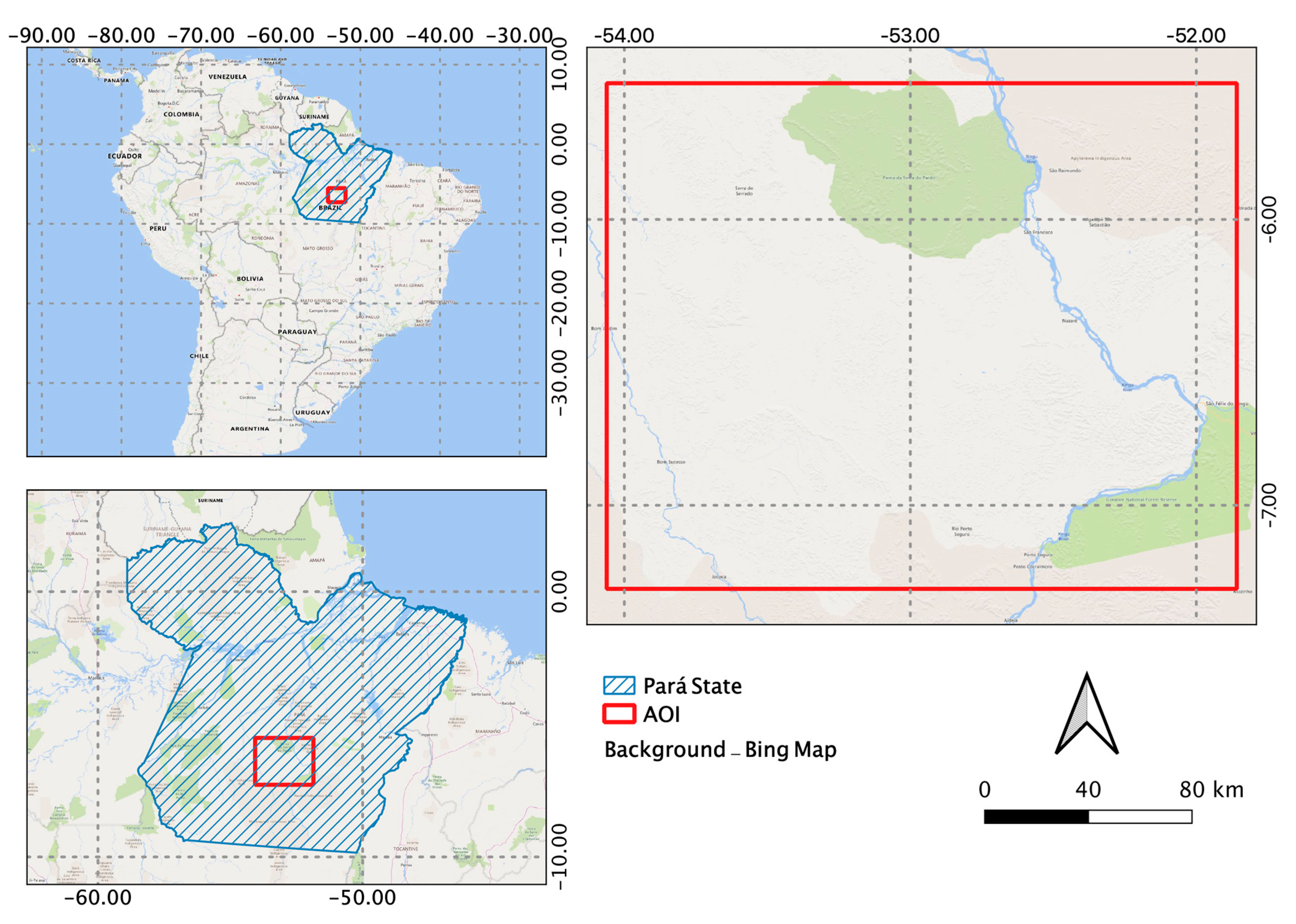
2.1. Study Area
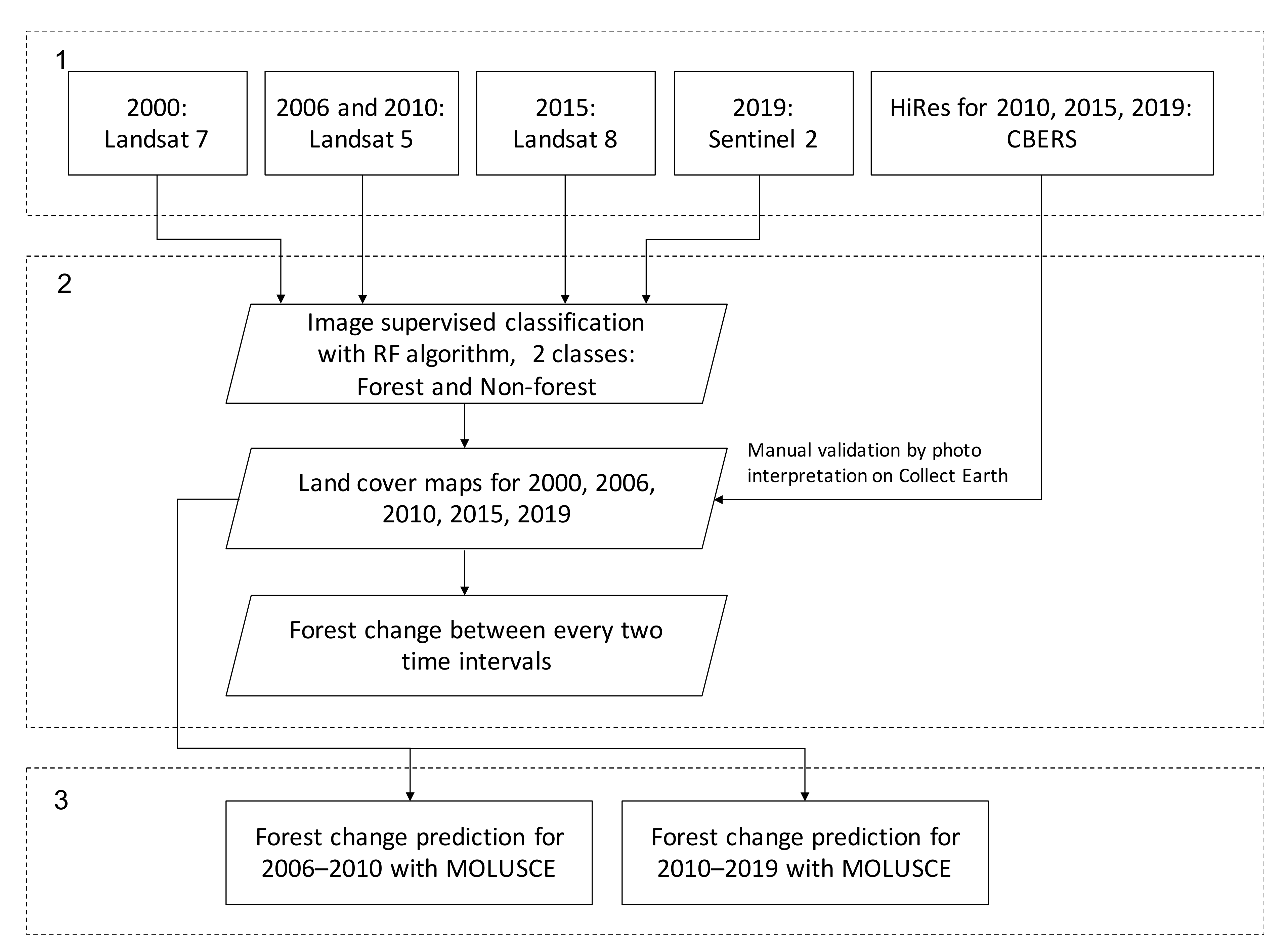
2.2. Data Used
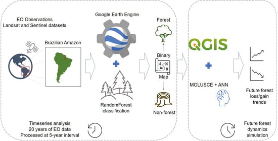
2.3. Classification Method
2.4. Processing Platform
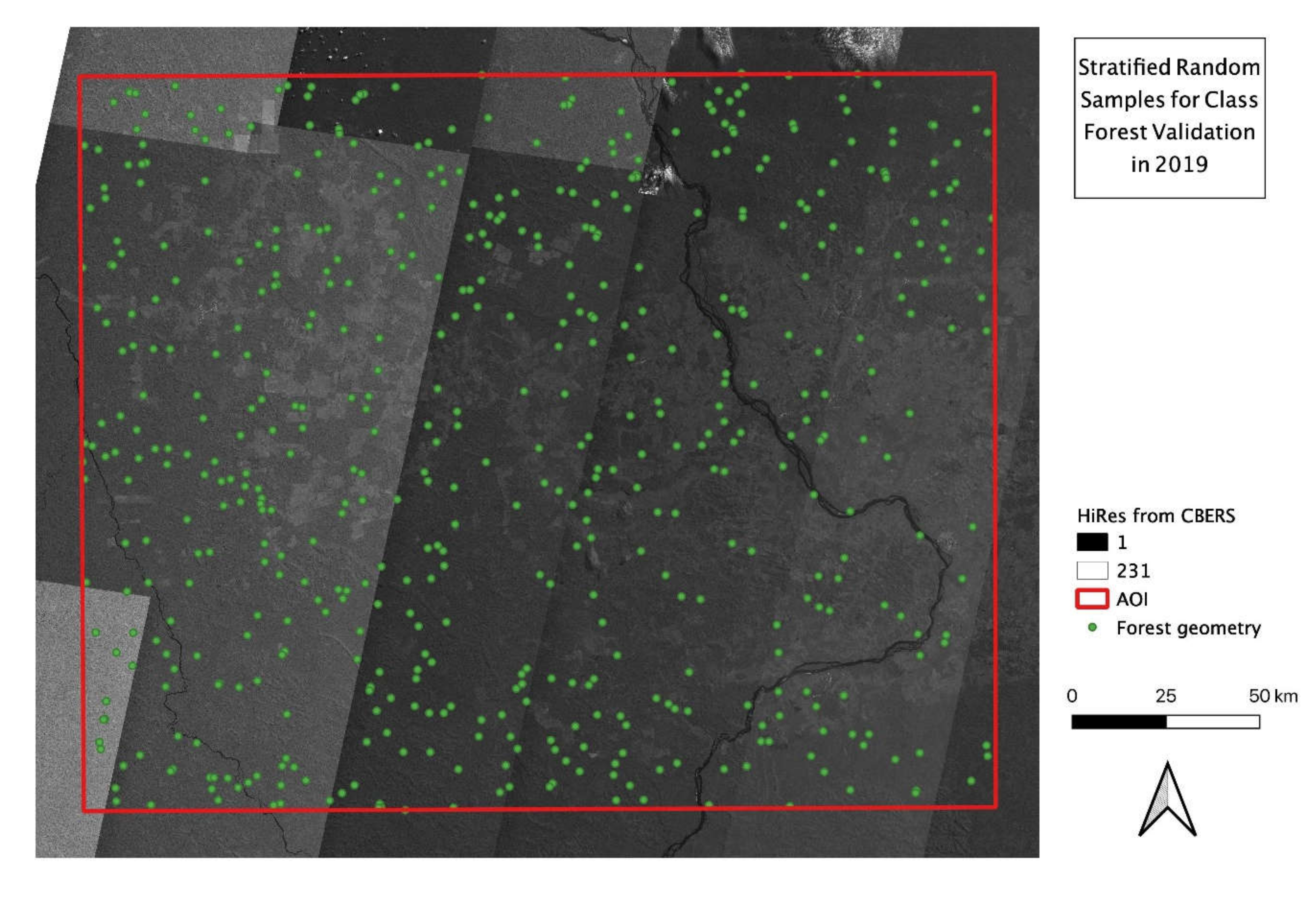
2.5. Validation
2.6. Simulating Forest Evolution
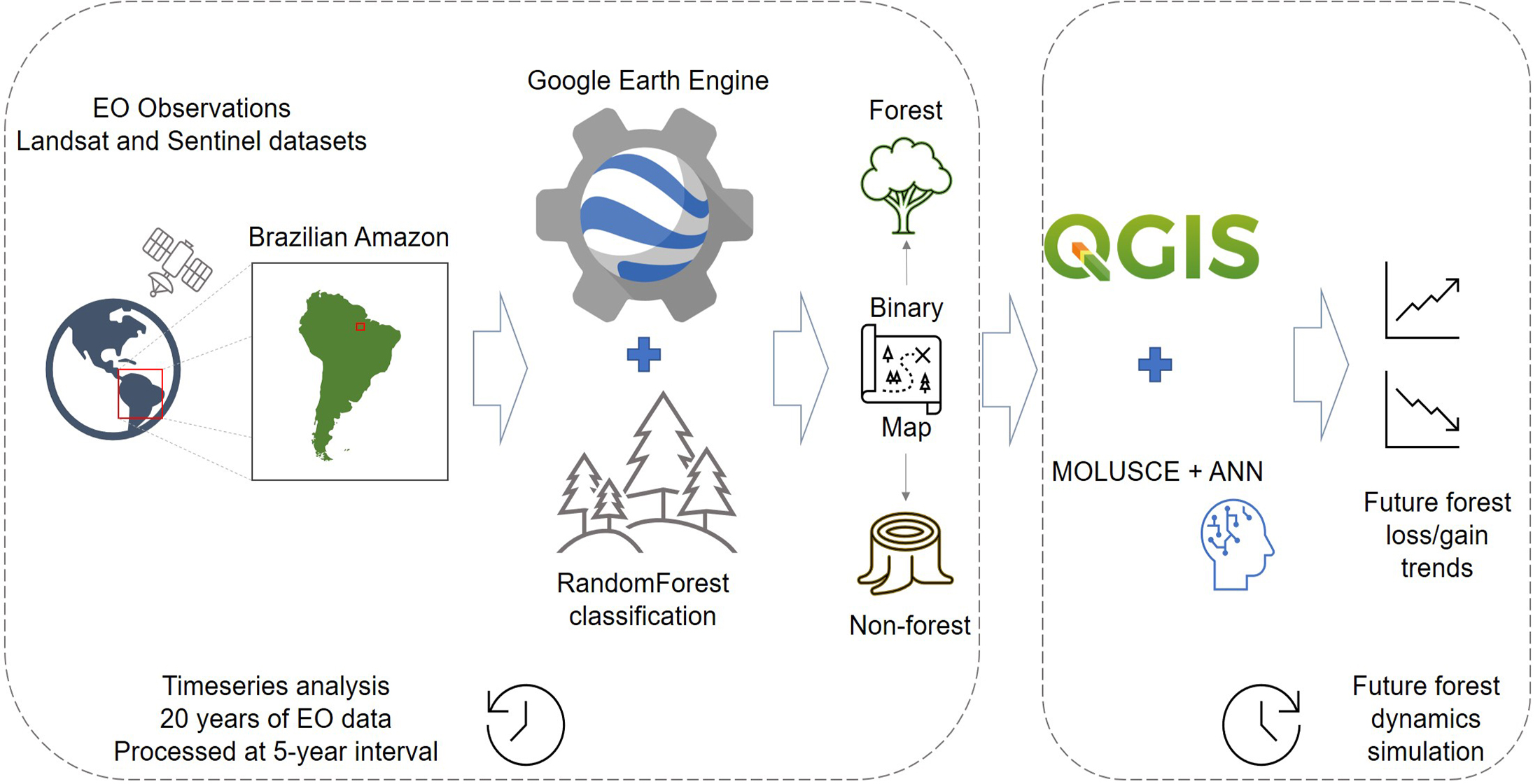
2.7. Workflow
3. Results
3.1. Classifications and Validations
3.1.1. Classification Results
3.1.2. Validation Results
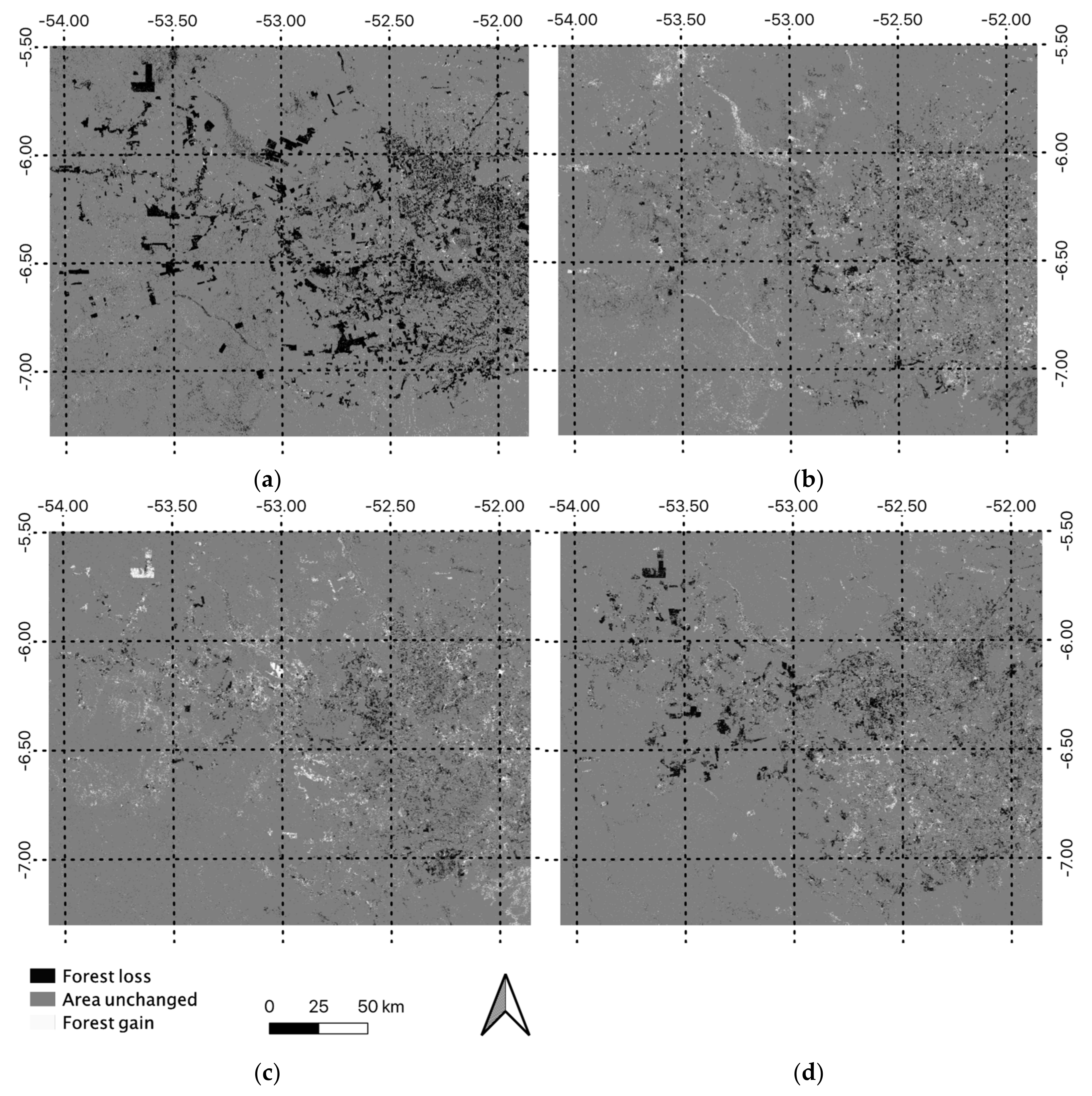
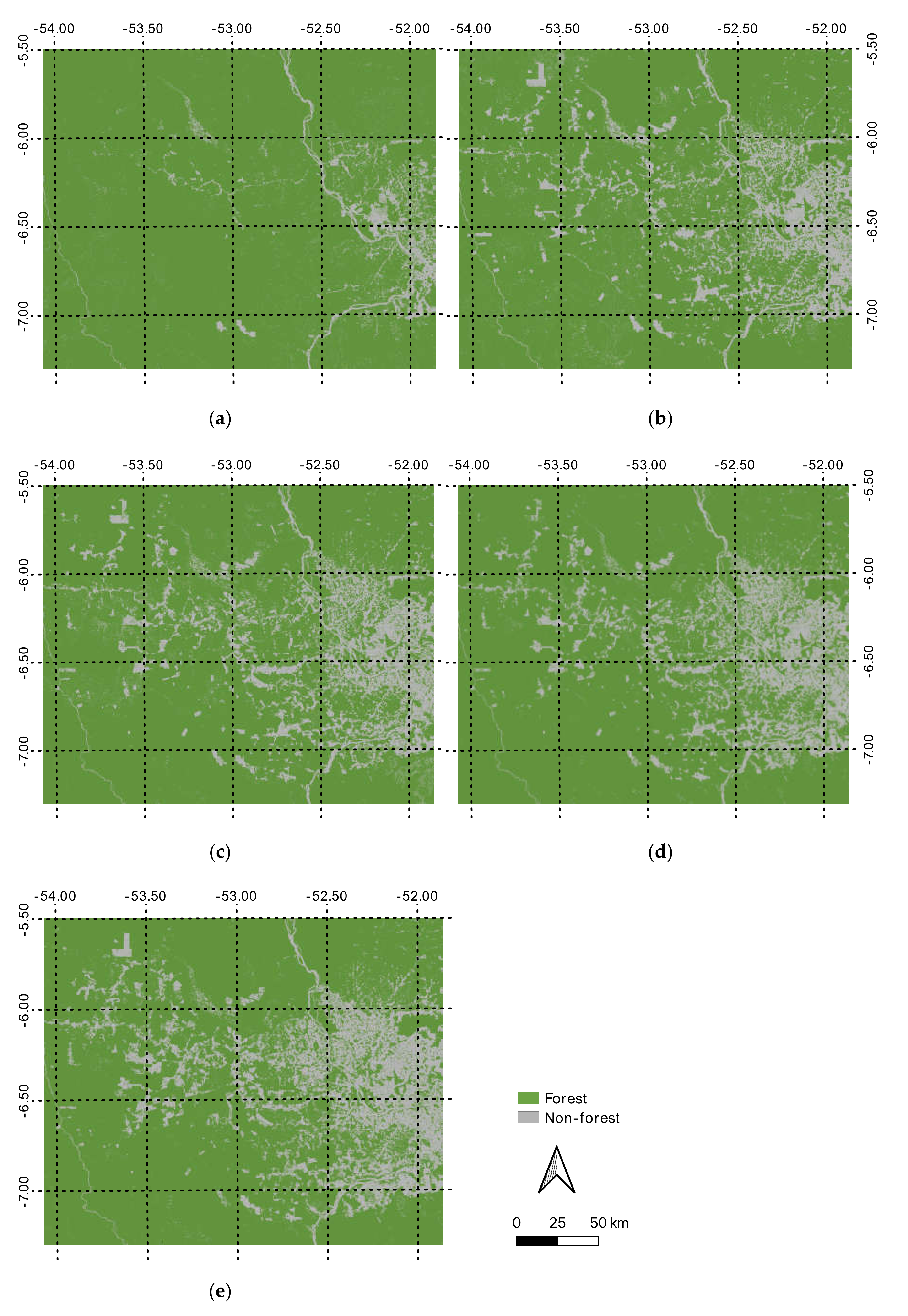
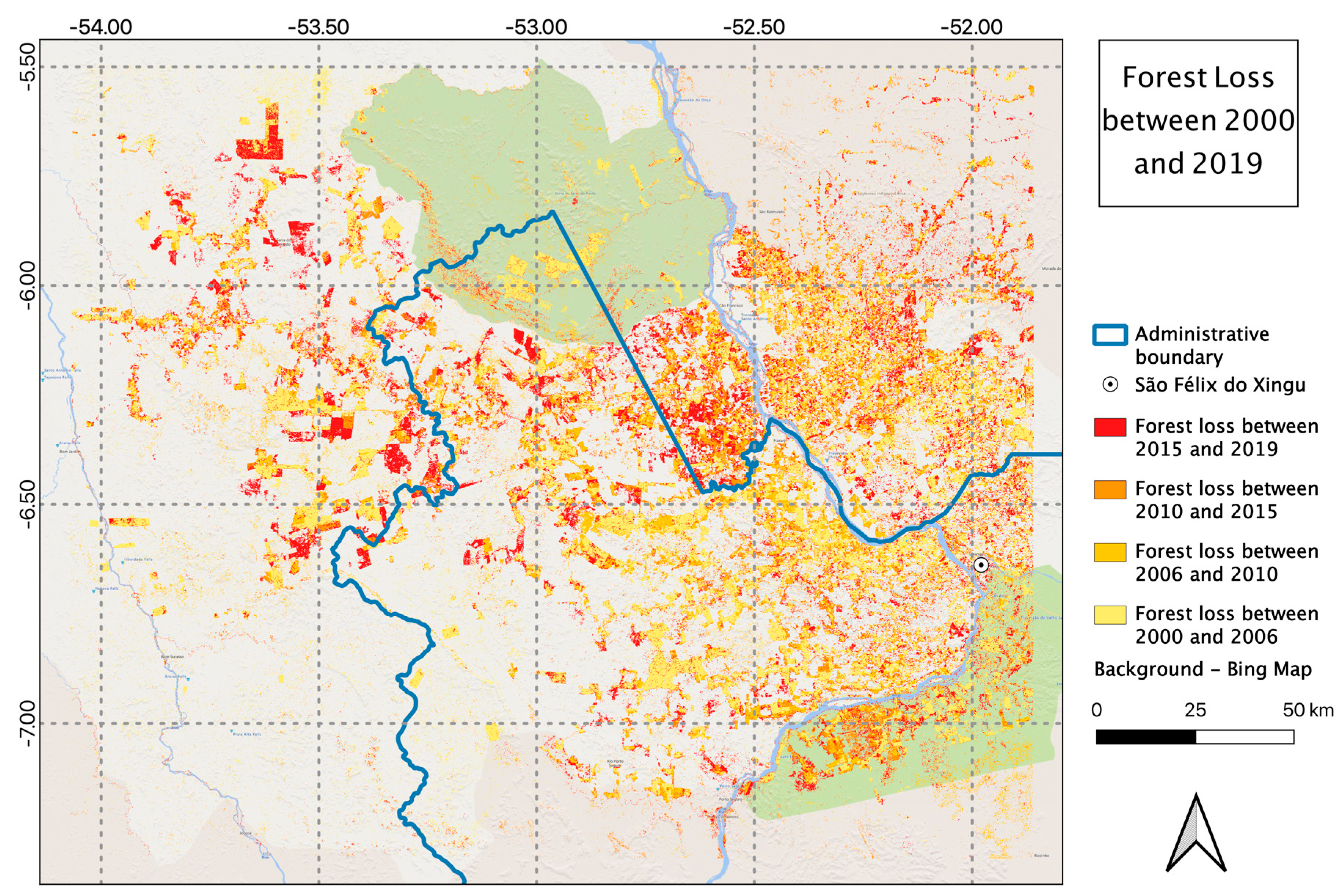
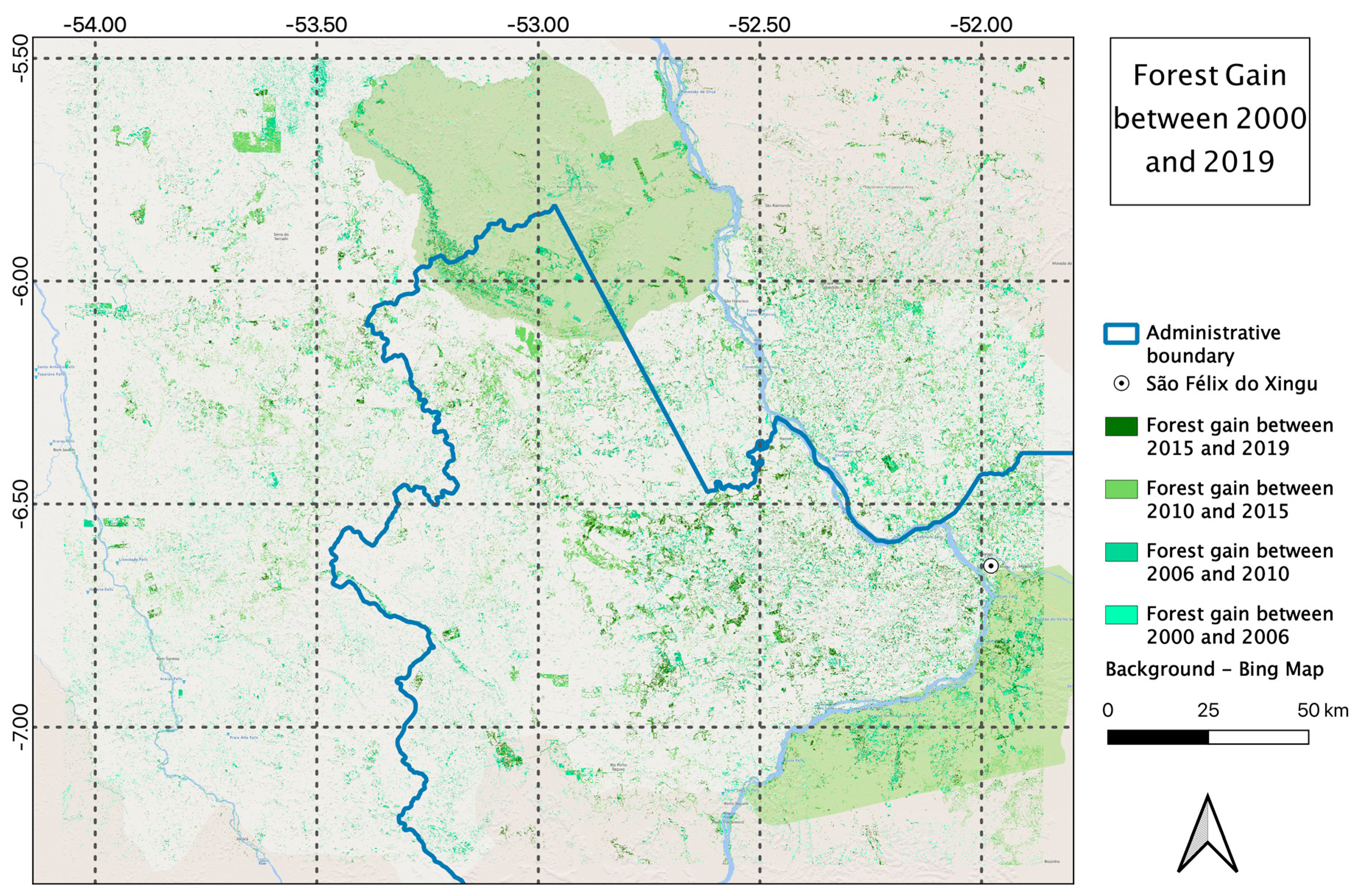
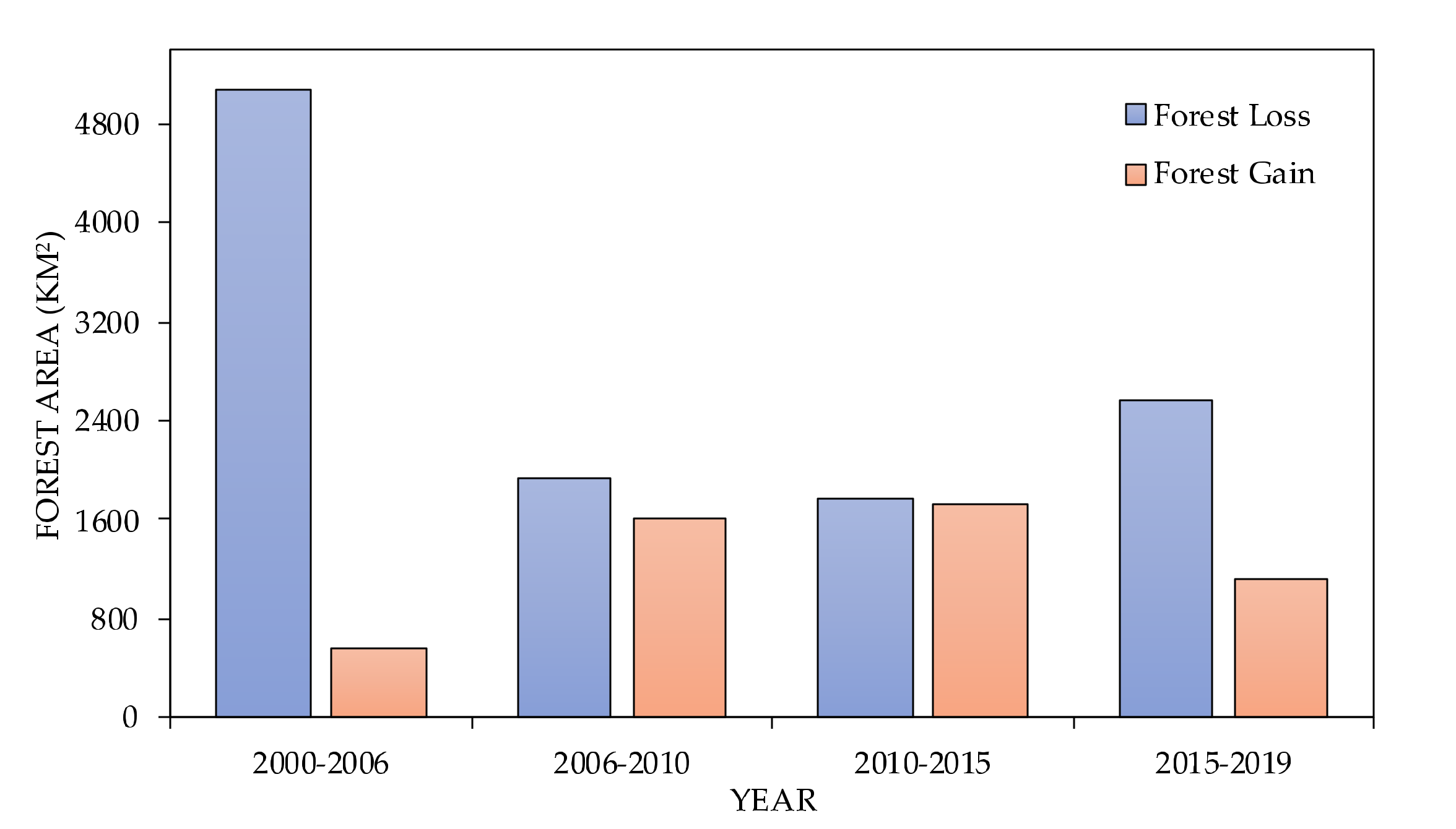
3.1.3. Forest Change
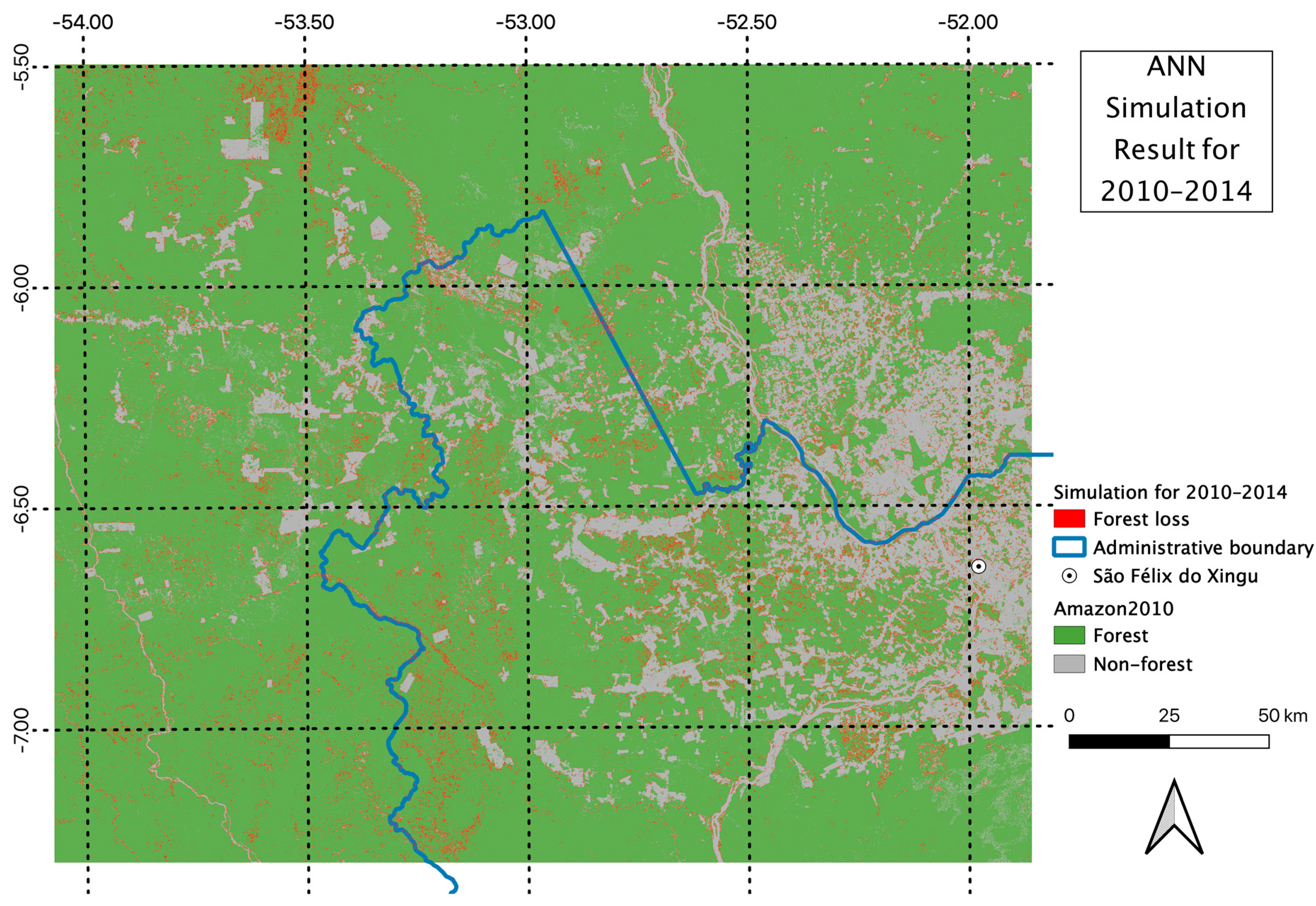
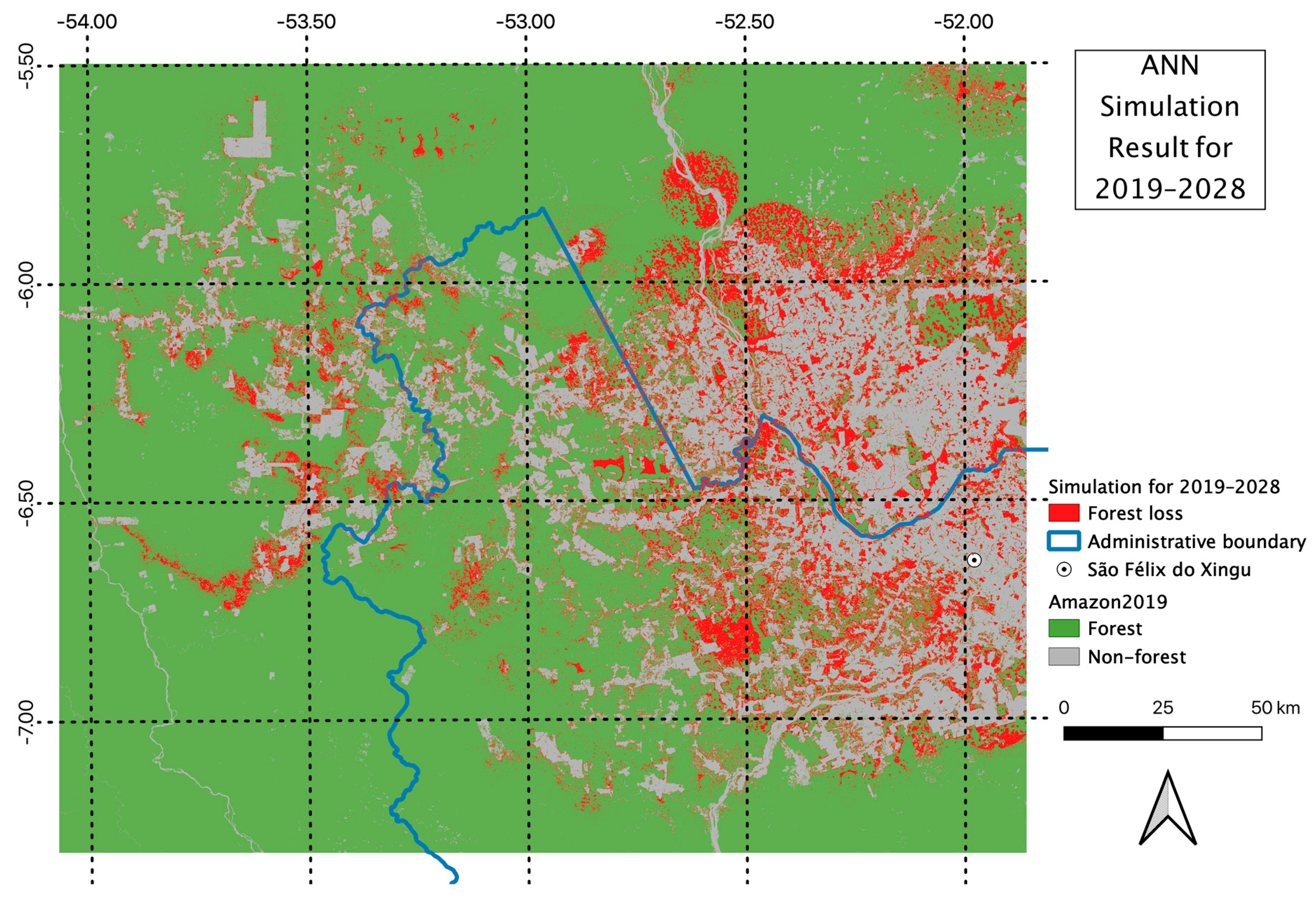
3.2. Simulation Results
4. Discussion
5. Conclusions
Author Contributions
Funding
Conflicts of Interest
References
- Geist, H.J.; Lambin, E.F. What Drives Tropical Deforestation. Glob. Environ. Chang. 2001, 4, 116. [Google Scholar] [CrossRef]
- Allen, J.C.; Barnes, D.F. The Causes of Deforestation in Developing Countries. Ann. Assoc. Am. Geogr. 1985, 75, 163–184. [Google Scholar] [CrossRef]
- Defries, R.S.; Rudel, T.; Uriarte, M.; Hansen, M. Deforestation driven by urban population growth and agricultural trade in the twenty-first century. Nat. Geosci. 2010, 3, 178–181. [Google Scholar] [CrossRef]
- Fearnside, P.M. Potential impacts of climatic change on natural forests and forestry in Brazilian Amazonia. For. Ecol. Manag. 1995, 78, 51–70. [Google Scholar] [CrossRef]
- Loreau, M.; Naeem, S.; Inchausti, P.; Bengtsson, J.; Grime, J.P.; Hector, A.; Hooper, D.U.; Huston, M.A.; Raffaelli, D.; Schmid, B.; et al. Ecology: Biodiversity and ecosystem functioning: Current knowledge and future challenges. Science 2001, 294, 804–808. [Google Scholar] [CrossRef] [PubMed] [Green Version]
- Kavian, A.; Azmoodeh, A.; Solaimani, K. Deforestation effects on soil properties, runoff and erosion in northern Iran. Arab. J. Geosci. 2014, 7, 1941–1950. [Google Scholar] [CrossRef]
- Zheng, F.-L. Effect of Vegetation Changes on Soil Erosion on the Loess Plateau. Pedosphere 2006, 16, 420–427. [Google Scholar] [CrossRef]
- D’Almeida, C.; Vörösmarty, C.J.; Hurtt, G.C.; Marengo, J.A.; Dingman, S.L.; Keim, B.D. The effects of deforestation on the hydrological cycle in Amazonia: A review on scale and resolution. Int. J. Climatol. 2007, 27, 633–647. [Google Scholar] [CrossRef]
- Nobre, C.A.; Sellers, P.J.; Shukla, J. Amazonian Deforestation and Regional Climate Change. J. Clim. 1991, 4, 957–988. [Google Scholar] [CrossRef] [Green Version]
- Fearnside, P.M.; Laurance, W.F. Tropical deforestation and greenhouse-gas emissions. Ecol. Appl. 2004, 14, 982–986. [Google Scholar] [CrossRef]
- Gibbs, H.K.; Herold, M. Tropical deforestation and greenhouse gas emissions. Environ. Res. Lett. 2007, 2, 045021. [Google Scholar] [CrossRef]
- Le Quéré, C.; Raupach, M.R.; Canadell, J.G.; Marland, G.; Bopp, L.; Ciais, P.; Conway, T.J.; Doney, S.C.; Feely, R.A.; Foster, P.; et al. Trends in the sources and sinks of carbon dioxide. Nat. Geosci. 2009, 2, 831–836. [Google Scholar] [CrossRef]
- Fuller, D.O. Tropical forest monitoring and remote sensing: A new era of transparency in forest governance. Singap. J. Trop. Geogr. 2006, 27, 15–29. [Google Scholar] [CrossRef]
- Manning, A.D.; Fischer, J.; Felton, A.; Newell, B.; Steffen, W.; Lindenmayer, D.B. Landscape fluidity—A unifying perspective for understanding and adapting to global change. J. Biogeogr. 2009, 36, 193–199. [Google Scholar] [CrossRef]
- Banskota, A.; Kayastha, N.; Falkowski, M.J.; Wulder, M.A.; Froese, R.E.; White, J.C. Forest Monitoring Using Landsat Time Series Data: A Review. Can. J. Remote Sens. 2014, 40, 362–384. [Google Scholar] [CrossRef]
- Cohen, W.B.; Yang, Z.; Kennedy, R. Detecting trends in forest disturbance and recovery using yearly Landsat time series: 2. TimeSync—Tools for calibration and validation. Remote Sens. Environ. 2010, 114, 2911–2944. [Google Scholar] [CrossRef]
- Fearnside, P.M. Deforestation in Brazilian Amazonia: History, Rates, and Consequences. Conserv. Biol. 2005, 19, 680–688. [Google Scholar] [CrossRef]
- Souza, C.M.; Roberts, D.A.; Monteiro, A.L. Multitemporal analysis of degraded forests in the southern Brazilian Amazon. Earth Interact. 2005, 9, 1–25. [Google Scholar] [CrossRef] [Green Version]
- Fearnside, P. Deforestation of the Brazilian Amazon. In Oxford Research Encyclopedia of Environmental Science; H.Shugart, Ed.; Oxford University Press: Oxford, UK, 2017. [Google Scholar] [CrossRef] [Green Version]
- Brown, D.S.; Brown, J.C.; Brown, C. Land occupations and deforestation in the Brazilian Amazon. Land Use Policy 2016, 54, 331–338. [Google Scholar] [CrossRef]
- Fujisaka, S.; Bell, W.; Thomas, N.; Hurtado, L.; Crawford, E. Slash-and-burn agriculture, conversion to pasture, and deforestation in two Brazilian Amazon colonies. Agric. Ecosyst. Environ. 1996, 59, 115–130. [Google Scholar] [CrossRef]
- Aldrich, S.; Walker, R.; Simmons, C.; Caldas, M.; Perz, S. Contentious Land Change in the Amazon’s Arc of Deforestation. Ann. Assoc. Am. Geogr. 2012, 102, 103–128. [Google Scholar] [CrossRef]
- Müller, H.; Griffiths, P.; Hostert, P. Long-term deforestation dynamics in the Brazilian Amazon—Uncovering historic frontier development along the Cuiabá–Santarém highway. Int. J. Appl. Earth Obs. Geoinf. 2016, 44, 61–69. [Google Scholar] [CrossRef]
- Cabral, A.I.R.; Saito, C.; Pereira, H.; Laques, A.E. Deforestation pattern dynamics in protected areas of the Brazilian Legal Amazon using remote sensing data. Appl. Geogr. 2018, 100, 101–115. [Google Scholar] [CrossRef]
- INPE PRODES—Coordenação-Geral de Observação da Terra. Available online: http://www.obt.inpe.br/OBT/assuntos/programas/amazonia/prodes (accessed on 30 July 2020).
- Duchelle, A.E.; Cromberg, M.; Gebara, M.F.; Guerra, R.; Melo, T.; Larson, A.; Cronkleton, P.; Börner, J.; Sills, E.; Wunder, S.; et al. Linking forest tenure reform, environmental compliance, and incentives: Lessons from redd+ initiatives in the brazilian amazon. World Dev. 2014, 55, 53–67. [Google Scholar] [CrossRef]
- Panta, M.; Kim, K.; Joshi, C. Temporal mapping of deforestation and forest degradation in Nepal: Applications to forest conservation. For. Ecol. Manag. 2008, 256, 1587–1595. [Google Scholar] [CrossRef]
- Shimabukuro, Y.E.; Arai, E.; Duarte, V.; Jorge, A.; dos Santos, E.G.; Gasparini, K.A.C.; Dutra, A.C. Monitoring deforestation and forest degradation using multi-temporal fraction images derived from Landsat sensor data in the Brazilian Amazon. Int. J. Remote Sens. 2019, 40, 5475–5496. [Google Scholar] [CrossRef]
- Liu, X.; Hu, G.; Chen, Y.; Li, X.; Xu, X.; Li, S.; Pei, F.; Wang, S. High-resolution multi-temporal mapping of global urban land using Landsat images based on the Google Earth Engine Platform. Remote Sens. Environ. 2018, 209, 227–239. [Google Scholar] [CrossRef]
- Rodriguez-Galiano, V.F.; Chica-Olmo, M.; Abarca-Hernandez, F.; Atkinson, P.M.; Jeganathan, C. Random Forest classification of Mediterranean land cover using multi-seasonal imagery and multi-seasonal texture. Remote Sens. Environ. 2012, 121, 93–107. [Google Scholar] [CrossRef]
- Pal, M. Random forest classifier for remote sensing classification. Int. J. Remote Sens. 2005, 26, 217–222. [Google Scholar] [CrossRef]
- Gislason, P.O.; Benediktsson, J.A.; Sveinsson, J.R. Random forests for land cover classification. Pattern Recognit. Lett. 2006, 27, 294–300. [Google Scholar] [CrossRef]
- Belgiu, M.; Drăgu, L. Random forest in remote sensing: A review of applications and future directions. ISPRS J. Photogramm. Remote Sens. 2016, 114, 24–31. [Google Scholar] [CrossRef]
- Liu, C.C.; Shieh, M.C.; Ke, M.S.; Wang, K.H. Flood prevention and emergency response system powered by Google Earth Engine. Remote Sens. 2018, 10, 1283. [Google Scholar] [CrossRef] [Green Version]
- Campos-Taberner, M.; Moreno-Martínez, Á.; García-Haro, F.J.; Camps-Valls, G.; Robinson, N.P.; Kattge, J.; Running, S.W. Global estimation of biophysical variables from Google Earth Engine platform. Remote Sens. 2018, 10, 1167. [Google Scholar] [CrossRef] [Green Version]
- He, M.; Kimball, J.S.; Maneta, M.P.; Maxwell, B.D.; Moreno, A.; Beguería, S.; Wu, X. Regional crop gross primary productivity and yield estimation using fused landsat-MODIS data. Remote Sens. 2018, 10, 372. [Google Scholar] [CrossRef] [Green Version]
- Fearnside, P.M. Deforestation in Brazilian Amazonia. In The Earth in Transition: Patterns and Processes of Biotic Impoverishment; Cambridge University Press: Cambridge, UK, 1990; Volume 530, pp. 211–234. [Google Scholar]
- Griffiths, P.; Jakimow, B.; Hostert, P. Reconstructing long term annual deforestation dynamics in Pará and Mato Grosso using the Landsat archive. Remote Sens. Environ. 2018, 216, 497–513. [Google Scholar] [CrossRef]
- Mertens, B.; Poccard-Chapuis, R.; Piketty, M.G.; Lacques, A.E.; Venturieri, A. Crossing spatial analyses and livestock economics to understand deforestation processes in the Brazilian Amazon: The case of São Félix do Xingú in South Pará. Agric. Econ. 2002, 27, 269–294. [Google Scholar]
- Martinez, L.L.; Fiedler, N.C.; Lucatelli, G.J. Analysis of the relationship between deforestation and hotspots. Case study in the municipal districts of Altamira and São Félix do Xingu in the State of Pará. Rev. Arvore 2007, 31, 695–702. [Google Scholar] [CrossRef] [Green Version]
- Jusys, T. Fundamental causes and spatial heterogeneity of deforestation in Legal Amazon. Appl. Geogr. 2016, 75, 188–199. [Google Scholar] [CrossRef]
- TerraBrasilis. Available online: http://terrabrasilis.dpi.inpe.br/app/dashboard/deforestation/biomes/legal_amazon/rates (accessed on 26 July 2020).
- Breiman, L. Random Forests. Mach. Learn. 2001, 45, 5–32. [Google Scholar] [CrossRef] [Green Version]
- Thanh Noi, P.; Kappas, M. Comparison of Random Forest, k-Nearest Neighbor, and Support Vector Machine Classifiers for Land Cover Classification Using Sentinel-2 Imagery. Sensors 2017, 18, 18. [Google Scholar] [CrossRef] [Green Version]
- Hayes, M.M.; Miller, S.N.; Murphy, M.A. High-resolution landcover classification using random forest. Remote Sens. Lett. 2014, 5, 112–121. [Google Scholar] [CrossRef]
- Mather, P.; Tso, B. Classification Methods for Remotely Sensed Data, 2nd ed.; Chemical Rubber Company Press: Boca Raton, FL, USA, 2016; ISBN 9781420090741. [Google Scholar]
- Tso, B.; Mather, P.M. Classification Methods for Remotely Sensed Data, 1st ed.; Taylor & Francis: London, UK, 2001; ISBN 9780203303566. [Google Scholar]
- Ho, T.K. The random subspace method for constructing decision forests. IEEE Trans. Pattern Anal. Mach. Intell. 1998, 20, 832–844. [Google Scholar] [CrossRef] [Green Version]
- Google Earth Engine Platform—Google Earth Engine. Available online: https://earthengine.google.com/platform (accessed on 25 July 2020).
- Shelestov, A.; Lavreniuk, M.; Kussul, N.; Novikov, A.; Skakun, S. Exploring Google earth engine platform for big data processing: Classification of multi-temporal satellite imagery for crop mapping. Front. Earth Sci. 2017, 5, 17. [Google Scholar] [CrossRef] [Green Version]
- Wang, G.; Liu, J.; He, G. A method of spatial mapping and reclassification for high-spatial- resolution remote sensing image classification. Sci. World J. 2013, 2013, 192982. [Google Scholar] [CrossRef] [PubMed]
- Gorelick, N.; Hancher, M.; Dixon, M.; Ilyushchenko, S.; Thau, D.; Moore, R. Google Earth Engine: Planetary-scale geospatial analysis for everyone. Remote Sens. Environ. 2017, 202, 18–27. [Google Scholar] [CrossRef]
- Bey, A.; Díaz, A.S.P.; Maniatis, D.; Marchi, G.; Mollicone, D.; Ricci, S.; Bastin, J.F.; Moore, R.; Federici, S.; Rezende, M.; et al. Collect earth: Land use and land cover assessment through augmented visual interpretation. Remote Sens. 2016, 81, 807. [Google Scholar] [CrossRef] [Green Version]
- FAO Collect Earth: Open Foris. 2018. Available online: http://www.openforis.org/tools/collect-earth.html (accessed on 6 September 2020).
- Stehman, S.V.; Czaplewski, R.L. Design and analysis for thematic map accuracy assessment: Fundamental principles. Remote Sens. Environ. 1998, 64, 331–344. [Google Scholar] [CrossRef]
- Stehman, S.V. Basic probability sampling designs for thematic map accuracy assessment. Int. J. Remote Sens. 1999, 20, 2423–2441. [Google Scholar] [CrossRef]
- Scepan, J. Thematic validation of high-resolution global land-cover data sets. Photogramm. Eng. Remote Sens. 1999, 65, 1051–1060. [Google Scholar]
- Stehman, S.V. Sampling designs for accuracy assessment of land cover. Int. J. Remote Sens. 2009, 30, 5243–5272. [Google Scholar] [CrossRef]
- Olofsson, P.; Foody, G.M.; Herold, M.; Stehman, S.V.; Woodcock, C.E.; Wulder, M.A. Good practices for estimating area and assessing accuracy of land change. Remote Sens. Environ. 2014, 148, 42–57. [Google Scholar] [CrossRef]
- Stadelman, W.J. Contaminants of liquid egg products. In Microbiology of the Avian Egg; Springer: Boston, MA, USA, 1994; pp. 139–151. [Google Scholar]
- Gismondi, M. MOLUSCE—An open source land use change analyst for QGIS. In Proceedings of the OSGeo’s Global Conference for Open Source Geospatial Software. Nottingham, UK, 17–21 September 2013. [Google Scholar]
- Wu, F. A linguistic cellular automata simulation approach for sustainable land development in a fast growing region. Comput. Environ. Urban Syst. 1996, 20, 367–387. [Google Scholar] [CrossRef]
- MOLUSCE—Modules for Land Use Change Evaluation·nextgis/molusce·GitHub. Available online: https://github.com/nextgis/molusce/blob/master/doc/en/QuickHelp.pdf (accessed on 4 September 2020).
- Export OpenStreetMap. Available online: https://www.openstreetmap.org/export#map=6/42.088/12.564 (accessed on 4 September 2020).
- Project MapBiomas—Collection 4.1 of Brazilian Land Cover & Use Map Series. Available online: https://mapbiomas.org (accessed on 6 September 2020).
- Souza, C.M.; Z. Shimbo, J.; Rosa, M.R.; Parente, L.L.; A. Alencar, A.; Rudorff, B.F.T.; Hasenack, H.; Matsumoto, M.; G. Ferreira, L.; Souza-Filho, P.W.M.; et al. Reconstructing Three Decades of Land Use and Land Cover Changes in Brazilian Biomes with Landsat Archive and Earth Engine. Remote Sens. 2020, 12, 735. [Google Scholar] [CrossRef]
- Saito, T.; Rehmsmeier, M. The precision-recall plot is more informative than the ROC plot when evaluating binary classifiers on imbalanced datasets. PLoS ONE 2015, 10, e0118432. [Google Scholar] [CrossRef] [PubMed] [Green Version]
- Yordanov, V.; Brovelli, M.A. Comparing model performance metrics for landslide susceptibility mapping. Int. Arch. Photogramm., Remote Sens. Spat. Inf. Sci. 2020, 43, 1277–1284. [Google Scholar] [CrossRef]
- Xiong, J.; Thenkabail, P.S.; Gumma, M.K.; Teluguntla, P.; Poehnelt, J.; Congalton, R.G.; Yadav, K.; Thau, D. Automated cropland mapping of continental Africa using Google Earth Engine cloud computing. ISPRS J. Photogramm. Remote Sens. 2017, 126, 225–244. [Google Scholar] [CrossRef] [Green Version]
- Midekisa, A.; Holl, F.; Savory, D.J.; Andrade-Pacheco, R.; Gething, P.W.; Bennett, A.; Sturrock, H.J.W. Mapping land cover change over continental Africa using Landsat and Google Earth Engine cloud computing. PLoS ONE 2017, 12, e0184926. [Google Scholar] [CrossRef] [PubMed]
- Hansen, M.C.; Potapov, P.V.; Moore, R.; Hancher, M.; Turubanova, S.A.; Tyukavina, A.; Thau, D.; Stehman, S.V.; Goetz, S.J.; Loveland, T.R.; et al. High-Resolution Global Maps of 21st-Century Forest Cover Change. New Ser. 2013, 342, 850–853. [Google Scholar] [CrossRef] [PubMed] [Green Version]
- Souza, C.M.; Siqueira, J.V.; Sales, M.H.; Fonseca, A.V.; Ribeiro, J.G.; Numata, I.; Cochrane, M.A.; Barber, C.P.; Roberts, D.A.; Barlow, J. Ten-year landsat classification of deforestation and forest degradation in the brazilian amazon. Remote Sens. 2013, 51, 5493. [Google Scholar] [CrossRef] [Green Version]
- Fearnside, P.M. Land-tenure issues as factors in environmental destruction in Brazilian Amazonia: The case of Southern Pará. World Dev. 2001, 29, 1361–1372. [Google Scholar] [CrossRef]
- Fearnside, P.M. Land-use Trends in the Brazilian Amazon Region as Factors in Accelerating Deforestation. Environ. Conserv. 1983, 10, 141–148. [Google Scholar] [CrossRef] [Green Version]
- Reis, E.J.; Blanco, F.A. Causes of Brazilian Amazon Deforestation; Springer: Dordrecht, The Netherlands, 2000; pp. 143–165. [Google Scholar]
- Brazilian Federal Government. Brasil Law of Public Forests Management (Lei de Gestão de Florestas Públicas); Brazilian Federal Government: Brasília, Brazil, 2006; pp. 1–9.
- Lipscomb, M.; Prabakaran, N. Property rights and deforestation: Evidence from the Terra Legal land reform in the Brazilian Amazon. World Dev. 2020, 129, 104854. [Google Scholar] [CrossRef]
- The National REDD+ Strategy. Available online: http://redd.mma.gov.br/en/the-national-redd-strategy (accessed on 26 July 2020).
- REDD+ Initiatives in the Amazon Basin Global Forest Atlas. Available online: https://globalforestatlas.yale.edu/amazon/conservation-initiatives/redd (accessed on 26 July 2020).
- Assunção, J.; Gandour, C.; Rocha, R. Deforestation Slowdown in the Legal Amazon: Prices or Policies? Executive Summary. Clim. Policy Initiat. 2015, 20, 697–722. [Google Scholar] [CrossRef] [Green Version]
- Presidência da república casa civil grupo permanente de trabalho interministerial. Plano de Acao para a Prevencao e Controle do Desmatamento na Amazonia Legal; 2009; p. 156. Available online: http://combateaodesmatamento.mma.gov.br/images/conteudo/PPCDAM_2aFase.compressed.pdf (accessed on 4 September 2020).
- Efforts for Prevention and Control of Deforestation. Available online: http://www.amazonfund.gov.br/en/prevention-control-deforestation (accessed on 19 July 2020).
- Reydon, B.P.; Fernandes, V.B.; Telles, T.S. Land governance as a precondition for decreasing deforestation in the Brazilian Amazon. Land Use Policy 2020, 94, 104313. [Google Scholar] [CrossRef]
- Carvalho, W.D.; Mustin, K.; Hilário, R.R.; Vasconcelos, I.M.; Eilers, V.; Fearnside, P.M. Deforestation control in the Brazilian Amazon: A conservation struggle being lost as agreements and regulations are subverted and bypassed. Perspect. Ecol. Conserv. 2019, 17, 122–130. [Google Scholar] [CrossRef]


| Satellite | Operational (as for 2020) | Year | Spatial Resolution | Bands |
|---|---|---|---|---|
| Landsat 5 | 1984–2012 | 2000 | 30 m | 1(Blue), 2(Green), 3(Red), 4(NIR) |
| Landsat 7 | 1999–Present | 2006 and 2010 | ||
| Landsat 8 | 2013–Present | 2015 | 2(Blue), 3(Green), 4(Red), 5(NIR) | |
| Sentinel-2 | 2015–Present | 2019 | 10 m | 2(Blue), 3(Green), 4(Red), 8(NIR) |
| CBERS 2B | 2007–2010 | 2010 | 2.7 m | Panchromatic |
| CBERS 4 | 2014–Present | 2015 & 2019 | 5 m |
| Reference (HiRe) | User Accuracy | ||||
|---|---|---|---|---|---|
| Forest | Non-forest | ||||
| 2010 | Classified (Landsat) | Forest | 521 | 13 | 0.98 |
| Non-forest | 37 | 496 | 0.93 | ||
| Producer accuracy | 0.93 | 0.97 | |||
| Overall accuracy | 0.95 | ||||
| Kappa | 0.91 | ||||
| Precision | 0.98 | ||||
| Recall | 0.93 | ||||
| AUCPRC | 0.95 | ||||
| 2015 | Classified (Landsat) | Forest | 526 | 8 | 0.99 |
| Non-forest | 36 | 497 | 0.93 | ||
| Producer accuracy | 0.94 | 0.98 | |||
| Overall accuracy | 0.97 | ||||
| Kappa | 0.94 | ||||
| Precision | 0.99 | ||||
| Recall | 0.94 | ||||
| AUCPRC | 0.96 | ||||
| 2019 | Classified (Sentinel) | Forest | 523 | 11 | 0.98 |
| Non-forest | 32 | 501 | 0.94 | ||
| Producer accuracy | 0.94 | 0.98 | |||
| Overall accuracy | 0.97 | ||||
| Kappa | 0.94 | ||||
| Precision | 0.98 | ||||
| Recall | 0.94 | ||||
| AUCPRC | 0.96 | ||||
| Year | Loss (km2)/Gain (km2) | Percentage (Loss/Gain) | Relative Percentage (Loss/Gain) | Cumulative Loss/Gain (km2) |
|---|---|---|---|---|
| 2000–2006 | 5081.90/570.28 | 10.28%/1.15% | ||
| 2006–2010 | 1942.71/1615.15 | 3.93%/3.27% | −61.77%/183.22% | 7024.61/2185.43 |
| 2010–2015 | 1779.41/1731.78 | 3.60%/3.50% | −5.41%/7.22% | 8804.02/3917.21 |
| 2015–2019 | 2569.81/1115.86 | 5.20%/2.26% | 44.42%/−35.57% | 11,373.83/4462.79 |
© 2020 by the authors. Licensee MDPI, Basel, Switzerland. This article is an open access article distributed under the terms and conditions of the Creative Commons Attribution (CC BY) license (http://creativecommons.org/licenses/by/4.0/).
Share and Cite
Brovelli, M.A.; Sun, Y.; Yordanov, V. Monitoring Forest Change in the Amazon Using Multi-Temporal Remote Sensing Data and Machine Learning Classification on Google Earth Engine. ISPRS Int. J. Geo-Inf. 2020, 9, 580. https://0-doi-org.brum.beds.ac.uk/10.3390/ijgi9100580
Brovelli MA, Sun Y, Yordanov V. Monitoring Forest Change in the Amazon Using Multi-Temporal Remote Sensing Data and Machine Learning Classification on Google Earth Engine. ISPRS International Journal of Geo-Information. 2020; 9(10):580. https://0-doi-org.brum.beds.ac.uk/10.3390/ijgi9100580
Chicago/Turabian StyleBrovelli, Maria Antonia, Yaru Sun, and Vasil Yordanov. 2020. "Monitoring Forest Change in the Amazon Using Multi-Temporal Remote Sensing Data and Machine Learning Classification on Google Earth Engine" ISPRS International Journal of Geo-Information 9, no. 10: 580. https://0-doi-org.brum.beds.ac.uk/10.3390/ijgi9100580