Supporting Policy Design for the Diffusion of Cleaner Technologies: A Spatial Empirical Agent-Based Model


Abstract
:1. Introduction
2. Materials and Methods
2.1. Literature Review
2.2. A Mixed Hybrid Agent-Based Model (ABM)
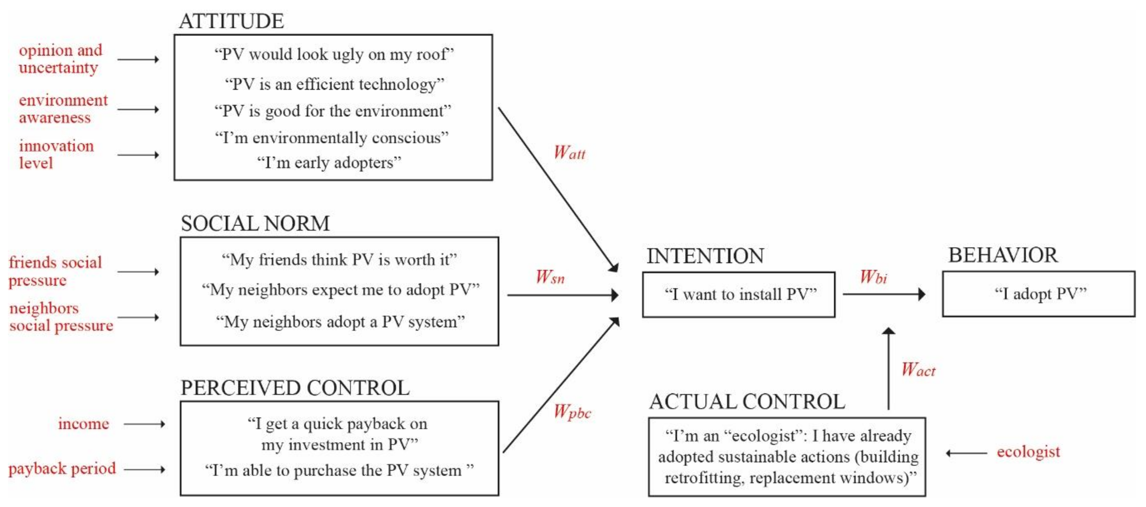
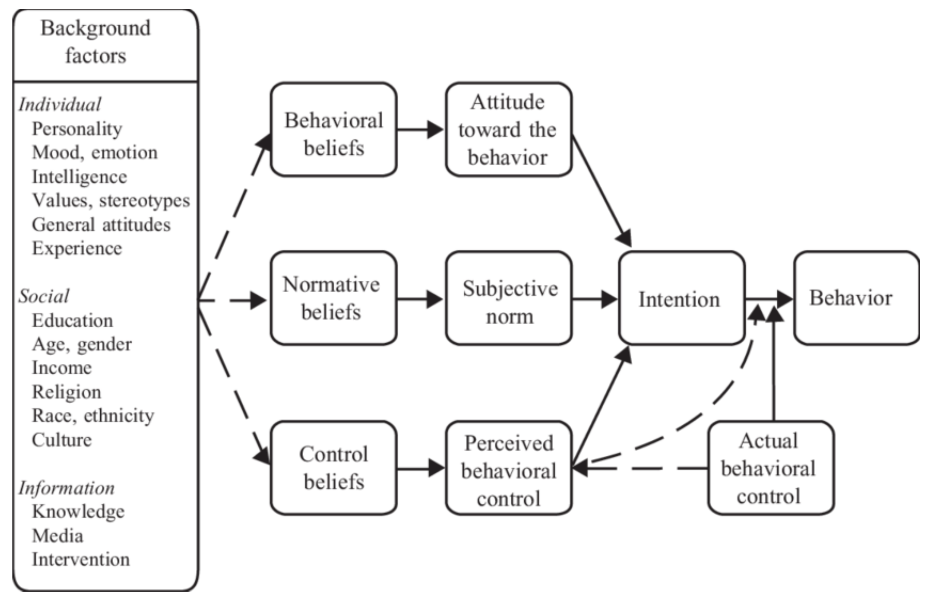
2.2.1. Theory of Planned Behavior
2.2.2. Opinion Formation
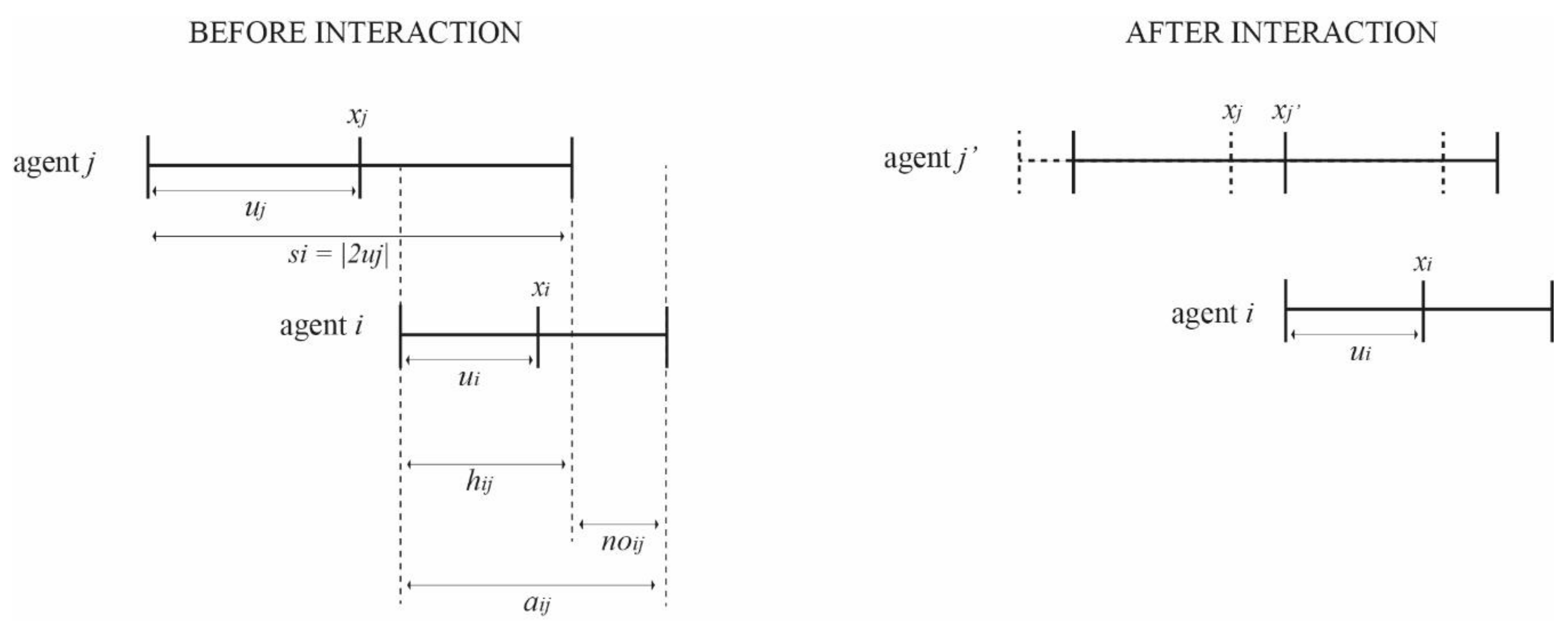
2.2.3. Social Network Theories
3. Application
- Model setup (entities, state and dynamic variables);
- Individual family adoption calculation;
- Policy mix framework.
3.1. Model Implementation and Variables Setting
- The global type refers to all entities responsible for the system-level implementation, such as electricity and policies (for the latter, we have considered both the current Italian regulatory framework and those policies designed by the authors for analyzing the possible increasing adoption of PV technology).
- The technological type is a specific type of global entity related to the characteristics of the energy technology analyzed in our model, i.e., the PV system.
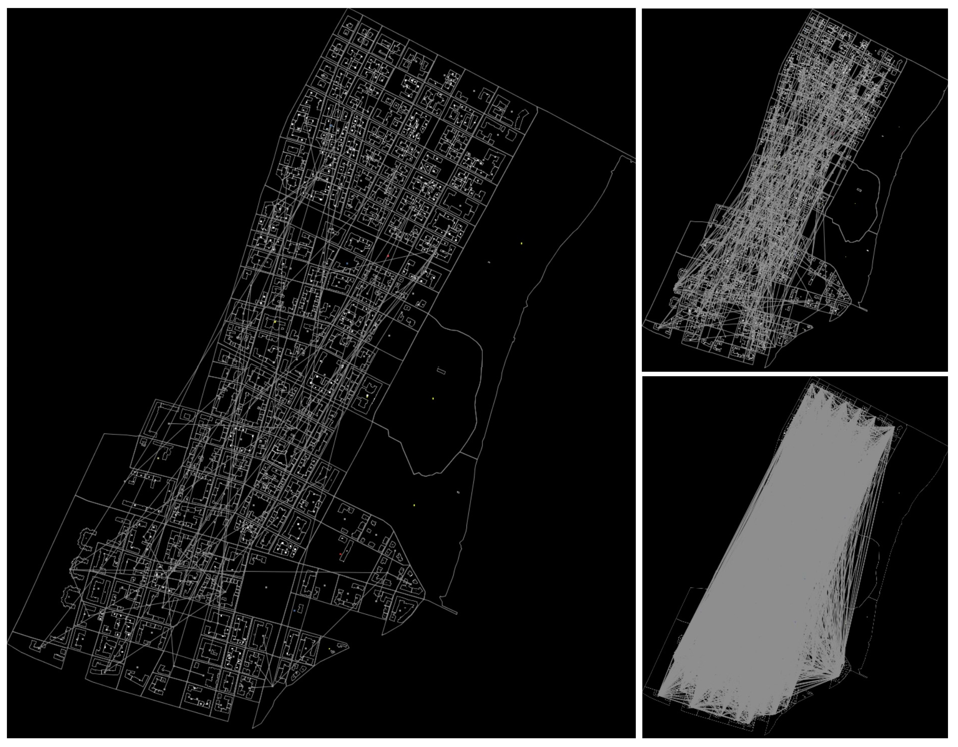
- The environmental type collects those entities which refer to the spatial characterization of the district. In the present research, it was considered only information about the location of buildings and the census block division, since more details are not necessary for our simulation model (such as building age, rooftop surface), even if available from municipality databases. However, these entities contain real-spatial data related to family characteristics and composition. In Netlogo, the building/census block representation was performed thanks to the GIS extension based on raster data performed in QGIS 3.4.14. Each raster has specific information on the family composition, level of instruction, job employment, nationality, and property status (owners or tenants). In this way, in Netlogo, the agents with their specific characteristic contained in the raster were “sprout” from their census blocks. Sprout is a specific command in Netlogo, which mainly refers to the agents sprouting from the related environment (patches).
- The agent type considers the single-family residential households distributed in the district. As described before, some characteristics of each family arise from the raster and represent the real-spatial distribution of specific families in the different census blocks. In this way, potential adopters are individual, heterogeneous agents representing the population of electricity consumers of the district.
- -
- Energy expenditure and energy need were defined based on the family composition. Data on the average energy expenditure for family composition at a national level were provided by ISTAT [51] and these values were simply converted into the energy need of each family as follows: energy need = energy expenditure * 12 months / electricity cost;
- -
- Status, innovation level and income are all static variables which are dependent on different combined features, such as education level, job occupation, number of components and nationality. The status classification was based on the social groups provided by ISTAT in its 2017 Annual Report [52]. The innovation level was assigned to the family based on its status class, which was, in turn, related to the diffusion of innovations classification provided by Rogers’ adopters categories [54]. Finally, the income was assigned as a normal distribution value for each status class. In particular, the ISTAT analysis [52] gives information on the equivalent income and the Gini coefficient of each class. The income was thus obtained by multiplying the latter value for the mean national income (equal to EUR 29,998 in Italy in 2017) and considering, as a standard deviation, the GINI coefficient for the income of the class. The same assumptions for the definition of status, innovation level and income have been made by Bottaccioli et al. (2019) and are synthetized in Table 4;
- -
- Environmental awareness is a static variable of the family which refers to the awareness of environmental problems. This variable represents how much a family is conscious and pro-active in adopting sustainable actions for the environment. This variable adds to the innovation and income level an alternative catalyst in the diffusion of eco-products and sustainable energy technologies (studies on this topic are, for example, [56,57]);
- -
- Opinion and uncertainty are two static variables defined at time 0 of the model, which represent the individual family household’s consideration on the PV technology. These variables, however, can change after interactive communication among the agents during the time flow. Based on the theoretical model of opinion formation and dynamic by Deffuant et al. (2002) [29] and Meadows and Cliff (2012) [53] (see Section 2), the distribution of opinions and uncertainties follow a random-flow distribution, between −1 and 1 for opinion and between 0 and 2 for uncertainty, respectively. In the assignment of uncertainties, it was set 0.1 as a minimum value, in order to avoid problems of values equal to 0.
3.2. Individual Family Adoption Calculation
3.2.1. Attitude Toward the Behavior (att)
- -
- Opinion (opi) is strictly related to the PV technology and, in particular, to the consideration that each agent has on the technology in itself (such “PV would look ugly on my roof?”, “PV is an efficient technology?”) (see for example [21,24]). The definition of agents’ opinions, as mentioned in the Methods, follow the RA theory. Every year, agents create their own networks, following the SWN theory (see Section 2.2.3), as shown in Figure 4. These networks, then, change every 5 years, simulating the variation of relations among people during the years. The assignment of the opinion (as for the uncertainty) did not depend on one or more background factors of the agents, but simply it was assigned to each agent as a random opinion between -1 and 1 (as for uncertainty between 0.1 and 2, where the minimum uncertainty 0 was excluded for avoiding problems in the calculation). As mentioned in the previous section, 1.2% families at time 0 have already adopted the PV; they represented the innovators (or extremists in the model) and, their opinion and uncertainty were set as follows: x >= 0.8 and u = 0.1. For the final formulation of the agent’s attitude, the opinion should be standardized. In the present analysis, an interval standardization was performed:
- -
- Environmental awareness (awenv) is a constant awareness between 0 and 1 (see, for example, [22]), where 0 represents low awareness on environmental problems, whereas 1 is high interest in the environmental issue. As for the opinion and uncertainty, also the environmental awareness was defined with a random distribution, without any dependence on other characteristics of the agent. This variable can change only when an agent was selected as a new ecologist over the lifespan.
- -
- Innovation level (inn) is the last component of the individual attitude of an agent and represents the propensity toward an innovation. This static variable depends on many characteristics, such as lifestyle, habits and personality, and for that reason, in our model, it was assigned to an agent based on their social role [21]. The innovation values vary between 1 to 5, where 1 means a low level of innovation, whereas 5 represents high innovativeness of the agent. For the innovation level, it is necessary to perform the interval standardization before the final calculation of the attitude.
3.2.2. Subjective Norm (sn)
3.2.3. Perceived Behavior Control
3.2.4. Actual Control
3.3. Policy Design
- -
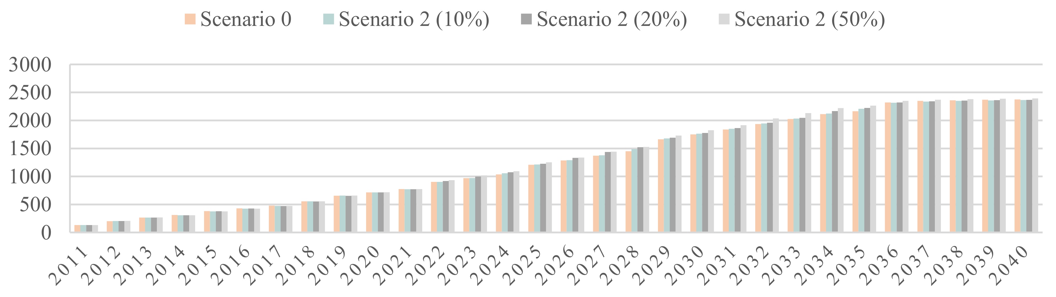
- Scenario 0 represents the state-of-the-art of the actual policy in the Italian context, which consists of the 50% tax relief on the investment cost for the purchase of PVs, deferred for ten years;
- -
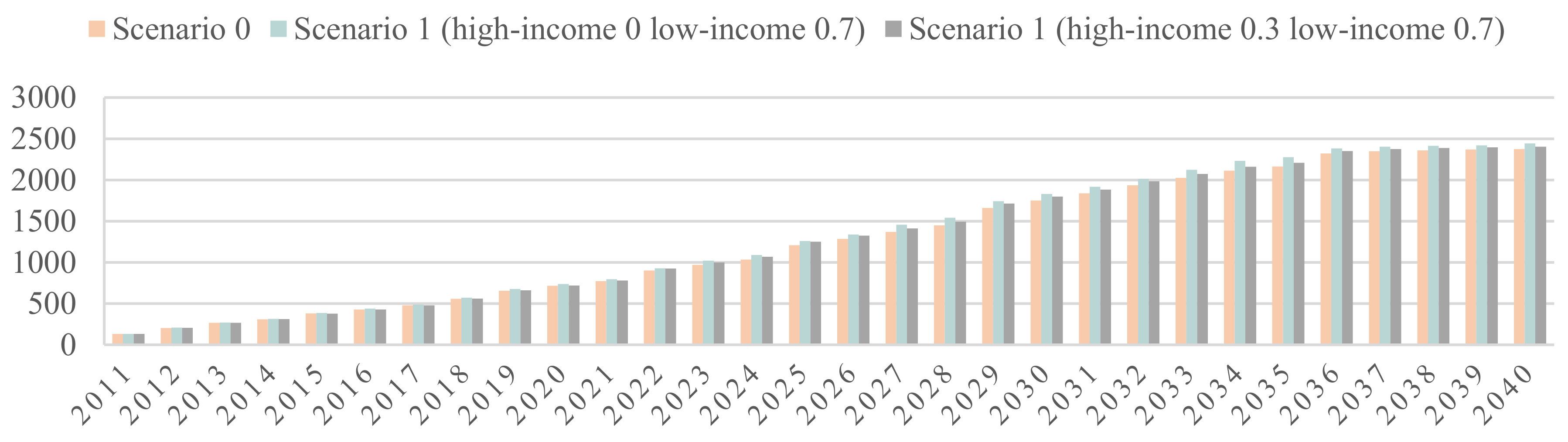
- Scenario 1 considers a different subsidies policy for low-income and high-income classes. Low-income people receive a subsidy equal to the 70% of the investment cost in ten years. For high-income people, two alternatives are tested: the first alternative considers no subsidies and the second one considers a subsidy equal to the 30% of the initial investment;
- -
- Scenario 2 introduces to the actual Italian policy, a discount voucher proposed by PV sellers:; this discount may be obtained by families if in their network there is at least one adopter. Different levels of discount were tested in the model (10%, 20% and 50%);
- -
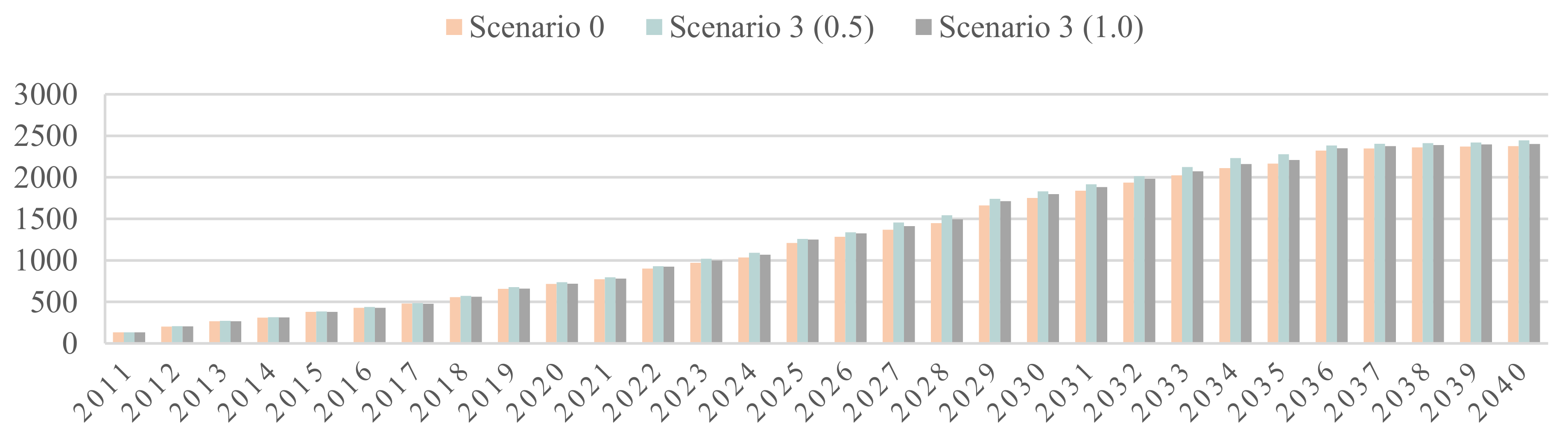
- Scenario 3 provides for an information campaign on environmental issues in order to increase the population awareness over this topic. A medium and a high information diffusion are tested, as a percentage increase in the level of environmental awareness of the individual, equal to 0.5 and 1.0, respectively;
- -
- Scenario 4 considers the development of an information campaign for increasing population awareness over the advantages of adopting the PV system. Additionally, in this case, two levels of information diffusion (medium and high) are considered, equal to 0.5 and 1.0, respectively.
4. Results
5. Discussion and Conclusions
Author Contributions
Funding
Acknowledgments
Conflicts of Interest
References
- Navarro-Yáñez, C.J.; Rodríguez-García, M.J. Urban policies as multi-level policy mixes. The comparative urban portfolio analysis to study the strategies of integral urban development initiatives. Cities 2020, 102, 102716. [Google Scholar] [CrossRef]
- Bottero, M.; D’Alpaos, C.; Dell’Anna, F. Boosting Investments in Buildings Energy Retrofit: The Role of Incentives. In Smart Innovation, Systems and Technologies, Proceedings of the International Symposium on New Metropolitan Perspectives, Reggio Calabria, Italy, 22–25 May 2018; Springer: Cham, Switzerland, 2018; pp. 593–600. [Google Scholar]
- Grubler, A.; Bai, X.; Buettner, T.; Dhakal, S.; Fisk, D.J.; Ichinose, T.; Keirstead, J.E.; Sammer, G.; Satterthwaite, D.; Schulz, N.B.; et al. Global Energy Assessment (GEA). In Urban Energy Systems; Johansson, T.B., Nakicenovic, N., Patwardhan, A., Gomez-Echeverri, L., Eds.; Cambridge University Press: Cambridge, UK, 2012; pp. 1307–1400. [Google Scholar]
- Kourtit, K.; Nijkamp, P. Big data dashboards as smart decision support tools for i-cities—An experiment on stockholm. Land Use Policy 2018, 71, 24–35. [Google Scholar] [CrossRef]
- Byrka, K.; Jedrzejewski, A.; Sznajd-Weron, K.; Weron, R. Difficulty is critical: The importance of social factors in modeling diffusion of green products and practices. Renew. Sust. Energ. Rev. 2016, 62, 723–735. [Google Scholar] [CrossRef] [Green Version]
- D’Alpaos, C.; Bragolusi, P. Multicriteria prioritization of policy instruments in buildings energy retrofit. Valori e Valutazioni 2018, 21, 15–25. [Google Scholar]
- MacAl, C.M.; North, M.J. Tutorial on agent-based modelling and simulation. In Proceedings of the Simulation Winter Conference, Orlando, FL, USA, 4 December 2005. [Google Scholar]
- Huang, Q.; Parker, D.C.; Filatova, T.; Sun, S. A review of urban residential choice models using agent-based modeling. Environ. Plan. B Plan. Des. 2014, 41, 661–689. [Google Scholar] [CrossRef]
- van Gent, W.P.C.; Musterd, S.; Ostendorf, W. Disentangling neighbourhood problems: Area-based interventions in western European cities. Urban Res. Pract. 2009, 21, 53–67. [Google Scholar] [CrossRef]
- Bottero, M.; Caprioli, C.; Cotella, G.; Santangelo, M. Sustainable cities: A reflection on potentialities and limits based on existing eco-districts in Europe. Sustainaility 2019, 11, 5794. [Google Scholar] [CrossRef] [Green Version]
- Luederitz, C.; Lang, D.J.; Von Wehrden, H. A systematic review of guiding principles for sustainable urban neighborhood development. Landsc. Urban Plan. 2013, 118, 40–52. [Google Scholar] [CrossRef]
- Parker, D.C.; Manson, S.M.; Janssen, M.A.; Hoffmann, M.J.; Deadman, P. Multi-agent systems for the simulation of land-use and land-cover change: A review. Ann. Assoc. Am. Geogr. 2003, 93, 314–337. [Google Scholar] [CrossRef] [Green Version]
- Railsback, S.F.; Grimm, V. Agent-Based and Individual-Based Modeling: A Practical Introduction; Princeton University Press: Princeton, NJ, USA, 2011. [Google Scholar]
- Sopha, B.M.; Klöckner, C.A.; Hertwich, E.G. Adoption and diffusion of heating systems in Norway: Coupling agent-based modeling with empirical research. Environ. Innov. Soc. Transit. 2013, 8, 42–61. [Google Scholar] [CrossRef]
- Snape, J.R.; Boait, P.J.; Rylatt, R.M. Will domestic consumers take up the renewable heat incentive? An analysis of the barriers to heat pump adoption using agent-based modelling. Energy Policy 2015, 85, 32–38. [Google Scholar] [CrossRef] [Green Version]
- Kiesling, E.; Günther, M.; Stummer, C.; Wakolbinger, L.M. Agent-based simulation of innovation diffusion: A review. Cent. Eur. J. Oper. Res. 2012, 20, 183–230. [Google Scholar] [CrossRef]
- Zhang, H.; Vorobeychik, Y. Empirically grounded agent-based models of innovation diffusion: A critical review. Artif. Intell. Rev. 2019, 52, 707–741. [Google Scholar] [CrossRef] [Green Version]
- Hesselink, L.X.W.; Chappin, E.J.L. Adoption of energy efficient technologies by households–Barriers, policies and agent-based modelling studies. Renew. Sustain. Energy Rev. 2019, 99, 29–41. [Google Scholar] [CrossRef]
- Haelg, L.; Waelchli, M.; Schmidt, T.S. Supporting energy technology deployment while avoiding unintended technological lock-in: A policy design perspective. Environ. Res. Lett. 2018, 13, 104011. [Google Scholar] [CrossRef] [Green Version]
- Lee, M.; Hong, T. Hybrid agent-based modeling of rooftop solar photovoltaic adoption by integrating the geographic information system and data mining technique. Energy Convers. Manag. 2019, 183, 266–279. [Google Scholar] [CrossRef]
- Schiera, D.S.; Minuto, F.D.; Bottaccioli, L.; Borchiellini, R.; Lanzini, A. Analysis of Rooftop Photovoltaics Diffusion in Energy Community Buildings by a Novel GIS- and Agent-Based Modeling Co-Simulation Platform. IEEE Access 2019, 7, 93404–93432. [Google Scholar] [CrossRef]
- Nuñez-Jimenez, A.; Knoeri, C.; Hoppmann, J.; Hoffmann, V.H. Can designs inspired by control theory keep deployment policies effective and cost-efficient as technology prices fall? Environ. Res. Lett. 2020, 15, 44002. [Google Scholar] [CrossRef]
- Zhao, J.; Mazhari, E.; Celik, N.; Son, Y.J. Hybrid agent-based simulation for policy evaluation of solar power generation systems. Simul. Model. Pract. Theory 2011, 19, 2189–2205. [Google Scholar] [CrossRef]
- Robinson, S.A.; Stringer, M.; Rai, V.; Tondon, A. GIS-integrated agent-based model of residential solar PV diffusion. In Proceedings of the 32nd USAEE/IAEE North American Conference, Anchorage, AK, USA, 28–31 July 2013; pp. 28–31. [Google Scholar]
- Rai, V.; Sigrin, B. Diffusion of environmentally-friendly energy technologies: Buy versus lease differences in residential PV markets. Environ. Res. Lett. 2013, 8, 14022. [Google Scholar] [CrossRef]
- Rai, V.; Robinson, S.A. Agent-based modeling of energy technology adoption: Empirical integration of social, behavioral, economic, and environmental factors. Environ. Model. Softw. 2015, 70, 163–177. [Google Scholar] [CrossRef] [Green Version]
- Clean Energy for all Europeans. Energy Policy Framework: European Commission. Available online: https://ec.europa.eu/energy/topics/energy-strategy-and-energy-union/clean-energy-all-europeans_en?redir=1 (accessed on 23 August 2020).
- Watts, D.; Strogatz, S. Collective dynamics of ‘small-world’networks. Nature 1998, 393, 440–442. [Google Scholar] [CrossRef] [PubMed]
- Deffuant, G.; Amblard, F.; Weisbuch, G.; Faure, T. How can extremism prevail? A study based on the relative agreement interaction model. J. Artif. Soc. Soc. Simul. 2002, 5, 4. [Google Scholar]
- Deffuant, G.; Neau, D.; Amblard, F.; Weisbuch, G. Mixing beliefs among interacting agents. Adv. Complex Syst. 2000, 3, 87–98. [Google Scholar] [CrossRef]
- Ajzen, I. The theory of planned behavior. Organ. Behav. Hum. Decis. Process. 1991, 50, 179–211. [Google Scholar] [CrossRef]
- Perri, C.; Giglio, C.; Corvello, V. Smart users for smart technologies: Investigating the intention to adopt smart energy consumption behaviors. Technol. Forecast. Soc. Chang. 2020, 155, 119991. [Google Scholar] [CrossRef]
- Abreu, J.; Wingartz, N.; Hardy, N. New trends in solar: A comparative study assessing the attitudes towards the adoption of rooftop PV. Energy Policy 2019, 128, 347–363. [Google Scholar] [CrossRef]
- Boeck, P.D.; Rosenberg, S. Hierarchical classes: Model and data analysis. Psychometrika 1988, 53, 361–381. [Google Scholar] [CrossRef]
- Ajzen, I. Constructing a TpB questionnaire: Conceptual and methodological considerations. J. Bus. Psychol. 2002. Available online: http://people.umass.edu/aizen/pdf/tpb.measurement.pdf (accessed on 23 August 2020).
- Galam, S.; Wonczak, S. Dictatorship from majority rule voting. Eur. Phys. J. B 2000, 18, 183–186. [Google Scholar] [CrossRef]
- Krause, U. A discrete nonlinear and non-autonomous model of consensus formation. In Communications in Difference Equations; Elaydi, S., Ladas, G., Popenda, J., Rakowski, J., Eds.; Gordon and Breach Publ.: Amsterdam, The Netherlands, 2000; pp. 227–236. [Google Scholar]
- Dittmer, J.C. Consensus formation under bounded confidence. Nonlinear Anal. Theory Methods Appl. 2001, 47, 4615–4621. [Google Scholar] [CrossRef]
- Hegselmann, R.; Krause, U. Opinion dynamics and bounded confidence models, analysis, and simulation. J. Artif. Soc. Soc. Simul. 2002, 5, 2. [Google Scholar]
- Goles, E.; Martinez, S. Neural and Automata Networks; Kluwer: Dordrecht, The Netherlands, 1990. [Google Scholar]
- Barabási, A.L.; Albert, R. Emergence of scaling in random networks. Science 1999, 286, 509–512. [Google Scholar] [CrossRef] [PubMed] [Green Version]
- De Sola Pool, I.; Milgram, S.; Newcomb, T.; Kochen, M. The Small World; Norwood, N.J., Ed.; Ablex Publ.: New York, NY, USA, 1989. [Google Scholar]
- Milgram, S. The small world problem. Psycology today. Psychology 1967, 2, 60–67. [Google Scholar]
- Guare, J. Six Degrees of Separation: A Play; Vintage: New York, NY, USA, 1990. [Google Scholar]
- Stokstad, E. Sustainable goals from UN under fire. Science 2015, 347, 702–703. [Google Scholar] [CrossRef]
- Tisue, S.; Wilensky, U. NetLogo: Design and implementation of a multi-agent modeling environment. In Proceedings of the Conference on Social Dynamics: Interaction, Reflexivity and Emergence, Chicago, IL, USA, 7–9 October 2004. [Google Scholar]
- Gestore Servizi Energetici: Rapporto Statistico Solare Fotovoltaico. Available online: https://www.gse.it/documenti_site/Documenti%20GSE/Rapporti%20statistici/Solare%20Fotovoltaico%20-%20Rapporto%20Statistico%202018.pdf (accessed on 23 August 2020).
- Eurostat: Electricity Prices by Type of User. Available online: https://ec.europa.eu/eurostat/tgm/table.do?tab=table&init=1&language=en&pcode=ten00117&plugin=1 (accessed on 23 August 2020).
- Dipartimento Attività Produttive: Lettera h, Articolo 16-bis del TUIR. Available online: https://www.brocardi.it/testo-unico-imposte-redditi/titolo-i/capo-i/art16.html?q=16+tuir&area=codici (accessed on 23 August 2020).
- ISTAT: Basi Territoriali e Variabili Censuarie. Available online: https://www.istat.it/it/archivio/104317 (accessed on 23 August 2020).
- ISTAT: Spese per Consumi. Available online: http://dati.istat.it/Index.aspx?DataSetCode=DCCV_SPEMEFAM (accessed on 28 September 2020).
- ISTAT: Rapporto Annuale 2017. Available online: https://www4.istat.it/it/archivio/199318 (accessed on 23 August 2020).
- Meadows, M.; Cliff, D. Reexamining the relative agreement model of opinion dynamics. J. Artif. Soc. Soc. Simul. 2012, 15, 4. [Google Scholar] [CrossRef] [Green Version]
- Rogers, E.M. The Diffusion of Innovations, 5th ed.; Free Press: New York, NY, USA, 2003. [Google Scholar]
- De Paoli, O.; Ricupero, M. Sistemi Solari Fotovoltaici e Termici. Strumenti per il Progettista; CELID: Torino, Italy, 2006. [Google Scholar]
- Mokha, A.K. Impact of Green Marketing Tools on Consumer Buying Behaviour. Asian J. Manag. 2018, 9, 168–174. [Google Scholar] [CrossRef]
- Paul, J.; Modi, A.; Patel, J. Predicting green product consumption using theory of planned behavior and reasoned action. J. Retail. Consum. Serv. 2016, 29, 123–134. [Google Scholar] [CrossRef]
- ISTAT: Popolazione e Ambiente: Preoccupazioni e Comportamenti dei Cittadini in Campo Ambientale. Available online: https://www4.istat.it/it/files/2015/12/Popolazione-e-ambiente.pdf?title=Popolazione+e+ambiente+-+22/dic/2015+-+Testo+integrale.pdf (accessed on 23 August 2020).
- Weiss, J.; Dunkelberg, E.; Vogelpohl, T. Improving policy instruments to better tap into homeowner refurbishment potential: Lessons learned from a case study in Germany. Energy Policy 2012, 44, 406–415. [Google Scholar] [CrossRef]
- Friege, J. Increasing homeowners’ insulation activity in Germany: An empirically grounded agent-based model analysis. Energy Build. 2016, 128, 756–771. [Google Scholar] [CrossRef]
- Friege, J.; Chappin, E. Modelling decisions on energy-efficient renovations: A review. Renew. Sustain. Energy Rev. 2014, 39, 196–208. [Google Scholar] [CrossRef] [Green Version]
- Anable, J.; Lane, B.; Kelay, T. An Evidence Base Review of Public Attitudes to Climate Change and Transport Behaviour; The Department for Transport: London, UK, 2006.
- Müller-Eie, D.; Bjørnø, L. The implementation of urban sustainability strategies: Theoretical and methodological implications for researching behaviour change. Int. J. Sustain. Dev. Plan. 2017, 12, 894–907. [Google Scholar] [CrossRef] [Green Version]


| Authors | Behavior Model 1 | Time 2 –Timeframe | Scale | Model Purpose | Policy | Variables | Geographic Information System (GIS) | Agents Initialization | Data Validation |
|---|---|---|---|---|---|---|---|---|---|
| Bottaccioli et al. (2019) [21] | TPB + RA + SWN | Q—20 years | District/ household | Policy design | (1to1) actual Italian regulatory framework vs. (1toM) joint self-consumption citizen (Clean Energy package [27]) |
| Yes, block scale | Italian statistics characteristics | Sensitivity of the attributes |
| Lee and Hong 2019 [20] | LR/PL + peer effect | Y—9 years | District/ household | Diffusion study | - |
| Yes, block scale | Census block data | Empirical data-driven behavioral rules of rooftop solar PV adoption |
| Nuñez-Jimenez et al. (2020) [22] | TF/UF + peer effects | Y—6 years | State | Policy evaluation | Adjusting incentives:
|
| No | Electricity consumers in Germany | Calibration of the attributes (historical cumulative installations between 1992 and 2016) |
| Rai and Robinson 2015 [26] | TPB (partial) + RA | Q—6 years | State/ household | Policy design |
|
| Yes, distribution with linear regression and results (city-level median) |
| Calibration of the attributes (empirical adoption levels between 2008 and 2013) |
| Rai and Sigrin 2013 [25] | FE | Y—25 years | State | Financial decision-process of consumers | - |
| No | Homogeneous (income, age, degree) | 5 Scenarios on electricity and PV system |
| Robinson et al. (2013) [24] | TPB + RA + SWN | Q | District/ household | Diffusion study | - |
| Yes, block scale | Social, economic, demographic and behavioral attributes of Austin (Texas) population (not more specified) | Calibration of the attributes based on historical data of adoption (2005–2008) |
| Zhao et al. 2011 [23] | TF | M—21 years | Region | Policy evaluation | Two incentives (Investment Credit Tax and Feed-in Tariff) |
| No | U.S. Census Bureau | Sensitivity on the attributes and real statistical data |
| Authors | Behavior Model | Time–Timeframe | Scale | Model Purpose | Policy | Variables | GIS | Agents Initialization | Data Validation |
|---|---|---|---|---|---|---|---|---|---|
| Our model | TPB + RA + SWN | Y—30 years | District | Policy design |
|
| Yes, block scale |
| Calibration of the attributes based on historical data of adoption (2011–2019) and sensitivity of the attributes |
| G/E/A/T 1 | Entities | Static Variables | Dynamic Variables | Setting | Source |
|---|---|---|---|---|---|
| G | electricity | electricity cost | median electricity cost in Italy | Eurostat database [48] | |
| G | electricity | electricity increment cost rate | −8% per year | GSE [47] | |
| G | policy | subsidies per kW | 0.5% of investment cost per 10 years | 2020 Italian Budget Law [49] | |
| E | census block | family distribution | number of families and their characteristics (family composition, level of instruction, job employment, nationality, and owners or tenants) | census block—municipality of Turin database 1:1000 (shp) + ISTAT census variables at census block [50] | |
| E | buildings | family distribution | number of families | building—municipality of Turin database 1:1000 (shp) | |
| A | family | number of components | 1–6 components | ISTAT census variables at the census block | |
| A | family | energy expenditure | median energy expenditure for n of components | ISTAT energy expenditure based on the number of family components [51] | |
| A | family | energy need | energy expenditure × 12 months/electricity cost | ||
| A | family | property status | n of property and rent families | ISTAT census variables at the census block | |
| A | family | employment/ unemployment | n of households employed and unemployed | ISTAT census variables at the census block | |
| A | family | nationality | n of foreign citizens | ISTAT census variables at the census block | |
| A | family | education level | illiterate, literate, primary school, secondary school, graduation | ISTAT census variables at the census block | |
| A | family | status | from 1 to 9 | [21,52]—Family classification for social group | |
| A | family | income | normal distribution based on equivalent income per each class × mean income of household (standard deviation based on the class Gini coefficient) | [21,52]—Family classification for social group | |
| A | family | PV adoption | true or false | ||
| A | family | opinion | opinion after interaction | random between −1 and 1 | [29,53] |
| A | family | uncertainty | uncertainty after interaction | random between 0.1 and 2 | [29,53] |
| A | family | environmental awareness | random between 0 and 1 | ||
| A | family | innovation level | 1–5 (based on the status) | [21,54] | |
| T | PV system | PV power | 3 kW | ||
| T | PV cost | EUR 2000 per kW | |||
| T | PV decreased rate cost | -0.08 per year | Italian trend 2 | ||
| T | reduction efficiency | 0.6 per year | De Paoli et al. [55] | ||
| T | maintenance and operational cost (O&M cost) | EUR 35 × kWh per year | Italian trend 3 | ||
| T | O&M increment cost rate | 0.02 | Italian trend 3 |
| ISTAT Social Group | Status | Roger’s Adopters Categories | Innovation Level | ISTAT Equivalent Income | ISTAT GINI Coefficient | Income |
|---|---|---|---|---|---|---|
| Ruling class (RC) | 9 | Innovators, Early adopters | 5 | 1.694 | 0.283 | Normal distribution: Equivalent income × National median income Standard deviation: Gini coefficient × National median income] |
| Clerk household (CH) | 8 | Early adopters | 4 | 1.323 | 0.257 | |
| Young blue collars (YB) | 7 | Early adopters, Early majority | 4 | 1.135 | 0.232 | |
| Silver pensioners (SP) | 6 | Early majority | 3 | 0.965 | 0.246 | |
| Low-income Italian households (LI) | 5 | Early majority, Late majority | 3 | 0.934 | 0.226 | |
| Lonely old ladies and young unemployed (LY) | 4 | Late majority | 3 | 0.804 | 0.324 | |
| Traditional provincial households (TP) | 3 | Late majority, Laggards | 2 | 0.758 | 0.282 | |
| Retired blue collars (RB) | 2 | Laggards | 2 | 0.707 | 0.290 | |
| Low income with foreigners (LF) | 1 | Laggards | 1 | 0.606 | 0.283 |
| 2011 | 2012 | 2013 | 2014 | 2015 | 2016 | 2017 | 2018 | 2019 | |
|---|---|---|---|---|---|---|---|---|---|
| PV adoption in Italy | 160,963 | 335,358 | 485,406 | 596,355 | 648,196 | 687,759 | 732,053 | 774,014 | 822,301 |
| PV adoption in the Metropolitan City Turin | 4293 | 8762 | 12,529 | 15,280 | 16,556 | 17,526 | 18,611 | 19,636 | 20,813 |
| % residential | 81% | ||||||||
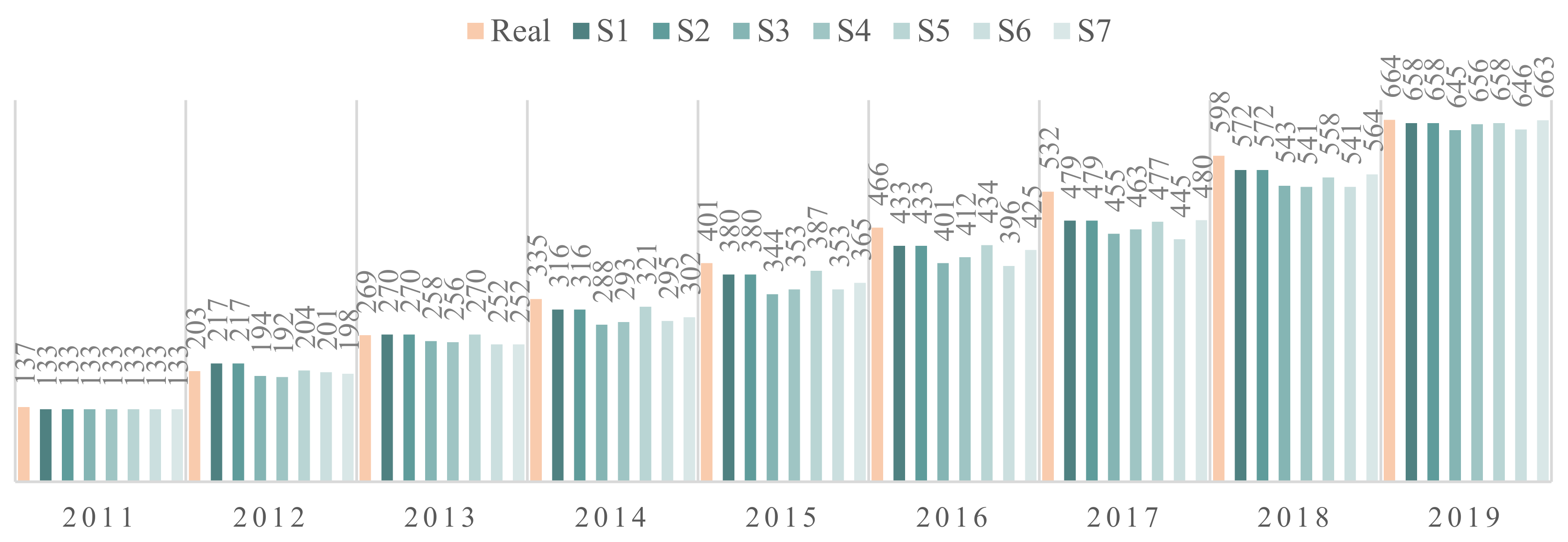
| % PV in San Salvario | 137 | 280 | 400 | 488 | 528 | 559 | 594 | 627 | 664 |
| % PV in San Salvario—omogeneous distribution per year | 137 | 203 | 269 | 335 | 401 | 466 | 532 | 598 | 664 |
| Static Variables | Dynamic Variables | Description |
|---|---|---|
| Property status | After the formation of the families with all their characteristics in the neighborhood, the model excludes all families with a rental contract, because these families cannot decide on adoption. This means that for every simulation run, the families excluded can, to some extent, change the configuration of the possible adopters. | |
| Opinion and uncertainty | These two variables are assigned with a random distribution whenever the model starts to run the simulation. | |
| Environmental awareness | Same as before, the number of ecologists at the beginning of the simulation, and every year, was the same. | |
| Attitude toward the behavior | Since this attribute depends on opinion and environmental awareness, the initial configuration of those variables affects the results of the attitude toward the behavior. | |
| Social norm | Since this attribute depends on opinion, environmental awareness and attitude toward the behavior, the initial configuration of those variables and attributes affects the results of the social norm. | |
| Interactions network | Interactions among agents followed SWN, choosing randomly a fixed number of agents (e.g., 6) inside and outside the radius selected (20 m). The model implemented asked agents to change their network every 5 years. This does not mean that an agent changes his/her opinion, attitude and social norm after five years; in fact, during this timeframe, agents are influenced also by the neighborhood as a whole, and this influence can also change opinion, attitude and norm in the network. |
© 2020 by the authors. Licensee MDPI, Basel, Switzerland. This article is an open access article distributed under the terms and conditions of the Creative Commons Attribution (CC BY) license (http://creativecommons.org/licenses/by/4.0/).
Share and Cite
Caprioli, C.; Bottero, M.; De Angelis, E. Supporting Policy Design for the Diffusion of Cleaner Technologies: A Spatial Empirical Agent-Based Model. ISPRS Int. J. Geo-Inf. 2020, 9, 581. https://0-doi-org.brum.beds.ac.uk/10.3390/ijgi9100581
Caprioli C, Bottero M, De Angelis E. Supporting Policy Design for the Diffusion of Cleaner Technologies: A Spatial Empirical Agent-Based Model. ISPRS International Journal of Geo-Information. 2020; 9(10):581. https://0-doi-org.brum.beds.ac.uk/10.3390/ijgi9100581
Chicago/Turabian StyleCaprioli, Caterina, Marta Bottero, and Elena De Angelis. 2020. "Supporting Policy Design for the Diffusion of Cleaner Technologies: A Spatial Empirical Agent-Based Model" ISPRS International Journal of Geo-Information 9, no. 10: 581. https://0-doi-org.brum.beds.ac.uk/10.3390/ijgi9100581