PolySimp: A Tool for Polygon Simplification Based on the Underlying Scaling Hierarchy


1
Research Institute for Smart Cities, School of Architecture and Urban Planning, Shenzhen University, Shenzhen 518060, China
2
Key Laboratory of Urban Land Resources Monitoring and Simulation, MNR, Shenzhen 518060, China
*
Author to whom correspondence should be addressed.
ISPRS Int. J. Geo-Inf. 2020, 9(10), 594; https://0-doi-org.brum.beds.ac.uk/10.3390/ijgi9100594
Submission received: 1 September 2020
/
Revised: 9 October 2020
/
Accepted: 9 October 2020
/
Published: 10 October 2020
(This article belongs to the Special Issue Geographic Complexity: Concepts, Theories, and Practices)
Abstract
:Map generalization is a process of reducing the contents of a map or data to properly show a geographic feature(s) at a smaller extent. Over the past few years, the fractal way of thinking has emerged as a new paradigm for map generalization. A geographic feature can be deemed as a fractal given the perspective of scaling, as its rough, irregular, and unsmooth shape inherently holds a striking scaling hierarchy of far more small elements than large ones. The pattern of far more small things than large ones is a de facto heavy tailed distribution. In this paper, we apply the scaling hierarchy for map generalization to polygonal features. To do this, we firstly revisit the scaling hierarchy of a classic fractal: the Koch Snowflake. We then review previous work that used the Douglas–Peuker algorithm, which identifies characteristic points on a line to derive three types of measures that are long-tailed distributed: the baseline length (d), the perpendicular distance to the baseline (x), and the area formed by x and d (area). More importantly, we extend the usage of the three measures to other most popular cartographical generalization methods; i.e., the bend simplify method, Visvalingam–Whyatt method, and hierarchical decomposition method, each of which decomposes any polygon into a set of bends, triangles, or convex hulls as basic geometric units for simplification. The different levels of details of the polygon can then be derived by recursively selecting the head part of geometric units and omitting the tail part using head/tail breaks, which is a new classification scheme for data with a heavy-tailed distribution. Since there are currently few tools with which to readily conduct the polygon simplification from such a fractal perspective, we have developed PolySimp, a tool that integrates the mentioned four algorithms for polygon simplification based on its underlying scaling hierarchy. The British coastline was selected to demonstrate the tool’s usefulness. The developed tool can be expected to showcase the applicability of fractal way of thinking and contribute to the development of map generalization.
1. Introduction
Dealing with global issues such environment, climate, and epidemiology for policy or decision making related to spatial planning and sustainable development requires geospatial information involving all types of geographic features at any level of details. In geographic information science, the term map generalization has been coined to address this need [1,2,3,4]. Simply put, map generalization keeps the major essential parts of the source data or a map at different levels of detail, thus excluding elements with less vital characteristics [5,6]. In other words, the purpose of generalization is to reduce the contents or complexity of a map or data to properly show the geographic feature(s) to a smaller extent. The generalization relates closely to the map scale, which refers to the ratio between the measurement on the map and the one in reality [7]. As the scale decreases, it is unavoidable to simplify and/or eliminate some geographic objects to make the map features discernible.
The generalization of a geographic object can be understood as the reduction of its geometric elements (e.g., points, lines, and polygons). The easiest way to conduct the simplification is removing points at a specified interval (i.e., every nth point; [8]); however, it may often fail to maintain the essential shape as it neglects the object’s global shape and neighboring relationships between its containing geometric elements. In order to keep as much as the original shape at coarser levels, related studies in the past several decades made great contributions from various perspectives, including smallest visible objects [9], effective area [10], topological consistency [11], deviation angles and error bands [12], shape curvature [13], multi-agent systems (AGENT project; [14,15]), and mathematical solutions such as a conjugate-gradient method [16], a Fourier-based approximation [17], etc. The accumulated repository of simplification methods and algorithms offer useful solutions to retain the core shape upon different criteria, but they seldom connect effectively simplified results with map scales.
In recent years, fractal geometry [18] has been proposed as the new paradigm for map generalization. Normant and Tricot [19] designed a convex-hull-based algorithm for line simplification while keeping the fractal dimension for different scales. Lam [20] pointed out that fractals could characterize the spatial patterns and effectively represent the relationships between geographic features and scales. Jiang et al. [5] developed a universal rule for map generalization that is totally within the fractal-geometric thinking. The rule is universal because there are far more small things than large ones globally over the geographic space and across different scales. This fact of an imbalanced ratio between large and small things—also known as the fractal nature of geographic features—has been formulated as scaling law [21,22,23]. Inspired by inherent fractal structure and scaling statistics of geographic features, Jiang [24] proposed that a large-scale map and its small-scale map have a recursive or nested relationship, and the ratio between the large and small map scales should be determined by the scaling ratio. In this connection, fractal nature, or scaling law could, to a certain degree, lead to a better guidance of the map generalization than Töpfer’s radical law [25], with respect to what needs to be generalized and the extent to which it can be generalized.
To characterize the fractal nature of geographic features, a new classification scheme called head/tail breaks [26] and its induced metric, the ht-index [27] can be effectively used to obtain the scaling hierarchy of numerous smallest, very few largest, and some in between the smallest and the largest (see more details in Section 2.2 and Appendix A). The scaling hierarchy derived from head/tail breaks can lead to automated map generalization from a single fine-grained map feature to a series of coarser-grained ones. Based on a series of previous studies, mapping practices, or map generalization in particular, can be considered to be head/tail breaks processes applied to geographic features or data. These kinds of thinking have received increased attention in the literature (e.g., [28,29,30,31,32]). However, given that fractal geometric thinking, especially linking with a map feature’s own scaling hierarchy, is still relatively new for map generalization, the practical difficulty is the lack of a tool to facilitate the computation of related fractal metrics that can guide the map generalization process.
The present work aims to develop such a tool, to advance the application of fractal-geometric thinking to the map generalization practices. The contributions of this paper can be described in terms of its three main aspects: (1) we introduced the geometric measures used in the previous study [5] to another three most popular polygon simplification algorithms; (2) we found out the fractal pattern of a polygonal feature is ubiquitous across selected algorithms, represented by the scaling statistics of geometric measures of all types; and (3) the developed tool (PolySimp) can make it possible to derive automatically a multiscale representation of a single polygonal feature based on head/tail breaks and its induced ht-index.
The rest of this paper is organized as follows. Section 2 reviews the related polygon simplification methods and illustrates the application of scaling hierarchy therein. Section 3 introduces the PolySimp tool regarding its user interface, functionality, and algorithmic consideration. In Section 4, the simplification of the British coastline is conducted using introduced algorithms and comparisons between different algorithms and geometric measures are made. The discussion is presented in Section 5, following with the conclusion in Section 6.
2. Methods
2.1. Related Algorithms for Polygon Simplification
The tool focuses on the polygon simplification, which is one of the major branches in the field of map generalization. As defined in the GIS literature [33], polygon simplification deals with the graphic symbology, leading to a simplification process of a polygonal feature that results in a multiscale spatial representation [34]. According to documentations of ArcGIS software [35] (ESRI 2020) and open-sourced platforms such as CartAGen [36,37], the geometric unit of a polygonal feature to be simplified is categorized by its points, bends, and other areal units (such as triangles and convex hulls), respectively.
The most common point-removal algorithm is probably the Douglas–Peucker (DP) algorithm [38], which can effectively maintain the essential shape of a polyline by finding and keeping the characteristic points while removing other unimportant ones. This algorithm runs in a recursive manner. Starting with a segment by linking two ends of a polyline, it detects the point with the maximum distance to that segment. If the distance is smaller than a given threshold, the points between the ends of the segment will be eliminated. If not, it keeps the furthest point and connects it with each segment’s end and repeats the previous steps on the newly created segments. The algorithm stops when all detected maximum distances are less than the given threshold. The DP algorithm can be applied by partitioning a polygon into two parts (left and right or up and down). One way to objectively partition a polygon is to use the segment linking the most distant point pair, such as the diagonal line of a rectangle. In this way, each part of a polygon can be processed as a polyline on which the DP algorithm can apply.
Evolved from point-removal approach, Visvalingam and Whyatt [10] put forward a triangle-based method (VW) to conduct the simplification. Each triangle is corresponding to a vertex and its two immediate neighbors, so that the importance of a vertex can be measured by the size of its pertaining triangle. The polygon simplification process is, therefore, iteratively removing those trivial vertices (small triangles). This method was further improved by using the triangle’s flatness, skewness, and convexity [39]. Later, Wang and Müller [40] proposed the bend simplify (BS) algorithm that defines bends as basic units for polyline/polygon simplification to better keep a polyline/polygon’s cartographic shape. Simply put, a line/polygon is made of numerous bends, each of which is composed of a set of consecutive points with the same sign of inflection angles. The following simplification process then becomes the recursive elimination of bends whose geometric characteristics are of little importance.
Another areal-unit-based algorithm is the hierarchical decomposition of a polygon (HD; [41]). It decomposes a polygon object into a set of minimum bounding rectangles or convex hulls. The algorithm also works in a recursive way. At each iteration, it constructs a convex hull for each polygon component, then extracts the subtraction/difference between the polygon component and its convex counterpart and uses it in the next iteration until the polygon component is small enough or its convex degree is larger than a preset threshold. Finally, all derived convex hulls are stored in a tree structure and marked with a corresponding iteration number. Based on the structured basic geometries, we can derive the original polygon using the following equation:
where k is the iteration number and is the convex hull set at iteration k.
The hierarchical decomposition algorithm provides a progressive transmission of a polygon object. According to the equation, it can obtain a polygon object at different levels of detail by adding or subtracting a convex hull set at related iteration. Note that the present study considered only a convex hull for further illustration.
2.2. Polygon Simplification Using Its Inherent Scaling Hierarchy
This study relied on the head/tail breaks method to conduct the generalization based on a polygonal feature’s scaling hierarchy. Head/tail breaks were initially developed as a classification method for data with a heavy-tailed distribution [26]. Given data with a heavy-tailed distribution, the arithmetic mean split up the data into the head (the small percentage with values above the mean, for example, <40 percent) and the tail (the large percentage with values below the mean). In this way, it recursively separated the head part into a new head and tail until the notion of far more smaller values than large ones was violated. The number of times that the head/tail division can be applied, plus 1, is the ht-index [27]. In other words, the ht-index indicates the number of times the scaling pattern of far more small elements than large ones recurs, thus capturing the data’s scaling hierarchy. In sum, data with a heavy-tailed distribution inherently possesses a scaling hierarchy, which equals the value of the ht-index: the number of recurring patterns of far more small things than large ones within the data.
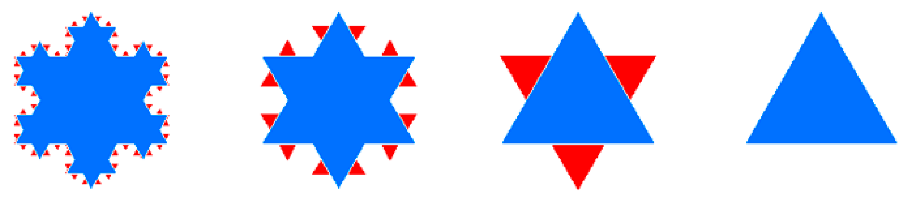
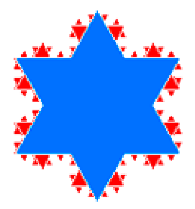
With the scaling hierarchy, the map generalization can be conducted using the head/tail breaks by recursively selecting the head part as the generalized result in the next level until the head part is no longer heavy-tailed [5]. It is simply because the head is self-similar to the whole data set that possesses a strikingly scaling hierarchy. Let us use the Koch snowflake to illustrate how head/tail breaks work for polygon simplification. Figure 1 shows the original snowflake, which contains 64 equilateral triangles of different sizes. More specifically, there were 48, 12, 3, and 1 triangle(s), with edge lengths of 1/27, 1/9, 1/3, and 1, respectively. The edge length of each triangle obviously followed a heavy-tailed distribution. Therefore, we could conduct the polygon simplification using head/tail breaks based on the edge length. The first mean is = 0.08, which split the triangles into 16 triangles above and 48 triangles below . Thus, those 16 triangles represent the head part (16/64 = 0.25, <40%) and were selected to be the first generalized result (Figure 1). The rest could be done in the same manner. The second mean = 0.21 helped to obtain a further simplified result consisting of the new head with four triangles (Figure 1). Finally, there was only one triangle above the third mean = 0.5, which was the last simplified result (Figure 1). It could be observed that the three levels of generalization were derived during the head/tail breaks process, which was consistent with the scaling hierarchy of all triangles.
As the above example shows, head/tail breaks offered an effective and straightforward way of simplifying a polygon object that bears the scaling hierarchy. However, the Koch snowflake is just a mathematical model under fractal thinking rather than a real polygon. The question then arises of how we can detect such a scaling pattern of an ordinary polygon whose scaling hierarchy is much more difficult to perceive than the Koch snowflake. Here we introduced three geometric measures: x, d, and the area of any polygon object relying on the aforementioned two algorithms.
Prior studies (e.g., [5,42]) have proposed the mentioned three measures based on the DP algorithm. As Figure 2a shows, x is the distance of the furthest point C from the segment linking two ends of a polyline (AF); d is the length of segment AF; and area equals the area of triangle ACF (x*d/2). In this study, we computed those three measures for VW, BS, and HD methods too, according to their own types of areal simplifying units. Taking the HD method as an example, as we know that the polygon will be decomposed into a set of convex hulls, the three measures can then be defined as Figure 2b illustrates: x is the furthest point C from the longest edge of a convex hull (AE); d is the length of longest edge AE; and area is the area of the convex hull ABCDE.
All three measures of four algorithms are derived in a recursive manner. Jiang et al. [5] showed that the measures x and x/d based on the DP method exhibit a heavy-tailed distribution. Thus, all the three measures of the DP method applying on the polygon feature are with a clear scaling hierarchy. For the other three algorithms, the size of the derived areal simplifying unit tends to be long-tailed distributed as well (see Figure A1 in Appendix A). Here we used the HD method again to exemplify: given that the original polygon was complex enough, the areas of all obtained convex hulls inevitably had scaling hierarchy, as do the other two measures since they were highly correlated with area. For a more intuitive description, the Koch snowflake was used again as a working example.
Figure 3 shows the decompositions of the Koch snowflake according to Equation (1). The process stops at Iteration 2 as all the polygon components are in the shape of triangles, the convex degree of which is 1. In total, there were 67 convex hulls. It can be clearly seen that there were more small convex hulls than large ones. If we apply head/tail breaks on the area of these convex hulls, it can be found that the scaling pattern recurs twice. Note that the Koch snowflake was far less complex than a cartographic polygon, which normally had more than 10 iterations. In this regard, we could detect the scaling pattern of decomposed convex hulls of a polygon object through x, d, and area based on the HD algorithm. This principle also works for VW and BS methods.
3. Development of a Software Tool: PolySimp
There are currently few tools with which to readily conduct the polygon simplification using four algorithms from the fractal perspective. To address this issue, we developed a software tool (referred to as PolySimp) in this study to facilitate the computation of introduced three measures and the implementation of generalization (Figure 4). The software tool was implemented with Microsoft Visual Studio 2010 with Tools for Universal Windows Apps. The generalization function was carried out by ArcEngine data types and interfaces of NET Framework 4.0. The software tool is designed to perform the following functions. The first is an input function. The tool should be capable of (a) loading a polygonal data and (b) presenting results to the inbuilt map viewer. The data files can be prepared in a format of Shapefile, which is the mostly widely used format in the current GIS environment. The second function is the output function, which is to generate the polygon simplification result based on the selected criteria; that is, the algorithm, the type of measure, and the level of detail to be generalized. When the generalization is completed, the result is shown in the second panel on the right-hand side. This software tool can be found in the Supplementary Materials.
As for algorithmic considerations, the software tool conducts polygon simplification by applying the head/tail breaks method to each of the three metrics, respectively. The flow charts in Figure 5 present the entire procedure of how the tool implements the functions. Given a series of the values for each of the three measures (x, d, and area) via four algorithms, we firstly generated those simplifying units; i.e., points, bends, triangles, or convex hulls. For the areal units, we made sure that the derived simplifying units were at the finest level for the sake of scaling hierarchy computation. As VW can associate each triangle with each point, we set only the rules for BS and HD algorithms: for BS, we detected the bend as long as the sign of inflection angle changed, so that the smallest bend could be a triangle; for HD, we set the stop condition on decomposing a polygon whereby every decomposed polygon component must be exactly convex, regardless of how small it is. Then, we kept those simplifying units whose values larger than the mean (in the head part), removing those with values smaller than the mean (in the tail). We believed that they were the critical part of a polygon and recursively keeping them could help to maintain the core shape at different levels. The process was continuous until the head part was no longer the minority (>40%); the head part recalculated every time a simplified polygon was generated. Note that when integrating the convex hulls in the head part using the HD method, whether a convex hull is added or subtracted depends on its iteration number (see Equation (1)).
4. Case Study and Analysis
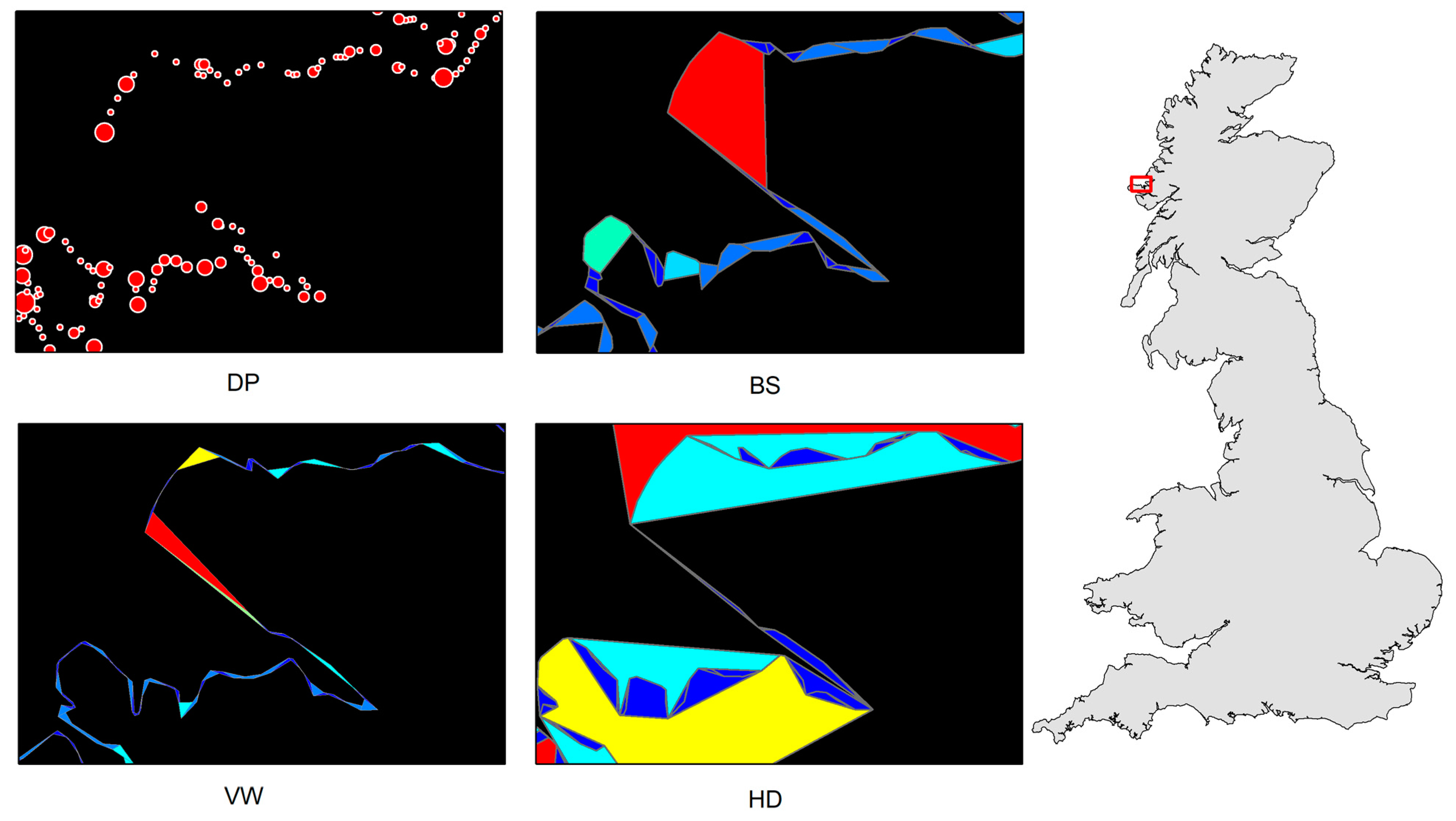
The British coastline was selected as a case study to illustrate how PolySimp works. As the shape of the British coastline (in part or in whole) has been widely used as case studies for DP, BS, and VW, we used it to demonstrate how the scaling hierarchy can be applied for polygon simplification and make comparisons accordingly. We derived the scaling hierarchies out of DP, BS, VW, and HD with better source data that contained 23,601 vertices (approximately 10 times more than the one used by [5]) using PolySimp. Both numbers of simplifying units for DP and VW were 23,601, which was consistent with the number of vertices; for BS and HD, there were 10,883 bends and 10,639 convex hulls, respectively (Figure 6). Table 1 shows the average running time of each level of detail between different simplification methods. It is worth noting that deriving convex hulls and reconstructing the simplified polygon for the HD algorithm was more costly than the other three, since it requires many polygon union/difference operations. After experimenting with the source data by calculating the three parameters of those simplifying units for each algorithm, we did the scaling analysis and found that all of them bore at least four scaling hierarchical levels, meaning that the pattern of far more small measures than large ones recurred no fewer than three times (Table 2). In other words, we observed a universal fractal or scaling pattern of the polygonal feature across four simplifying algorithms.
The scaling hierarchical levels correspond with levels of detail of the coastline. The top five levels of simplified polygons from four algorithms are presented in Figure 7. Due to different types of geometric units, the number of source vertices retained at each level differs dramatically from one algorithm to another (Table 3). To be specific, the BS method maintains the most points (on average, almost 45% of points are kept at each level), followed by VW (36%), HD (35%), and DP (23%). For each algorithm, it should be stressed that the number of points dropped more sharply if we used area to control the generalization, leading to the fewest levels of details. In contrast, using parameter x can generate most levels. Not only the number of points, but also do the generalized shapes differ between each other. Despite the simplified results at the fifth level, the polygonal-unit-based methods (especially VW and HD) can help to maintain a smoother and more natural shape than the point-unit-based algorithm (DP).
5. Discussion
To demonstrate the polygon simplification tool based on the underlying scaling hierarchy, we applied the tool on the British coastline. The study brought the predefined three geometric measures—x, d, and area—from the DP method to the other three methods; i.e., VW, BS, and HD methods, respectively. Each of the three measures in four algorithms is heavy-tailed distributed. Such a scaling pattern implies that the fractal nature does not exist only in the mathematical models (such as the Koch snowflake), but also in a geographic feature. With the fat-tailed statistics, head/tail breaks can be used as a powerful tool for deriving the inherent scaling hierarchy and help to partition the bends, triangles, and convex hulls into the heads and tails in a recursive manner. Those areal elements in the head are considered critical components of the polygon and then selected for further operations. Consequently, we found that most of the simplified shapes are acceptable at top several levels, which supports the usefulness of fractal-geometric thinking on cartographic generalization. Based on the findings, we further discussed the results and insights we obtained from this study.
For a more in-depth investigation, we computed the area (S), the perimeter (P), and the shape factor (P/S) for each simplified result. Figure 8 shows how they change respectively regarding each algorithm with different parameters. With three types of computed metrics (S, P, and P/S), we could measure and compare the performance of different simplification methods guided by the underlying scaling hierarchy. Ideally, the curve of each metric would be flat at each level of detail, meaning that the simplified polygon shapes are maintained to the maximum extent of the original one. In other words, a steep curve could indicate an unpleasant distortion (e.g., level 3 of the DP method in Figure 7c and Figure 8c). In general, we could observe from Figure 8 that VW and HD methods could capture a more essential shape across different levels than DP and BS, irrespective of the metric type. It should be noted that the metric curve of BS appeared to be flatter than that of VW or HD in some cases (e.g., Figure 8i); however, the simplified result at each level using the BS method kept many more points (about 50%) than that using either VW or HD (Table 3). In this connection, BS was less efficient. On the opposite, the large slopes of the metric curves of DP may often be caused by the dramatic drop of points. Therefore, we conjectured that the results of VW and HD algorithms achieved a good balance between the number of characteristic points and the core shape of the polygon, leading to a better performance in this study.
Based on the comparison of the results, the shapes of such a complicated boundary are best maintained using the VW and HD methods with x, even at the last level. Area turns out to be the worst parameter in this regard because it leads to fewer levels of details and improper shapes (Figure 7 and Figure 8). Presumably, area works as x times d so it weakens the effect of any single measure. To explain why, we again used the Koch snowflake. Figure 1 shows that the generalization process is guided by d, and it would be the same result if using x. However, using the area will result in a different series of generalization since more triangles will be eliminated in the first recursion (Figure 9); this explains why the number of vertices dropped more significantly than the other two measures. As x is a better parameter than d, we conjectured that the height captured more characteristics of an irregular geometry than its longest edge. This warrants further study.
It deserves to be mentioned that all algorithms work in a recursive way. The process of each algorithm can be denoted as a tree structure, of which a node represents a critical point or an areal element of a polygonal feature. Despite the node difference, the tree structures between two algorithms are also fundamentally different. The tree from the DP algorithm is a binary tree [43], since a line feature is split iteratively into two parts by the furthest point and two ends of the base segment. Thus, each node can have at most two children. Other algorithms, however, produce a N-ary tree without such a restriction, for that the number of children of each parent node is dependent on how many bends, triangles or concave parts belong to the node. In this respect, the areal-unit-based simplifying algorithms generate a less rigid and more organic tree than the point-based one, which is more in line with the complex structure of a geographic object that is naturally formulated. Therefore, the simplification results from VW and HD are more natural and smoother than that from DP.
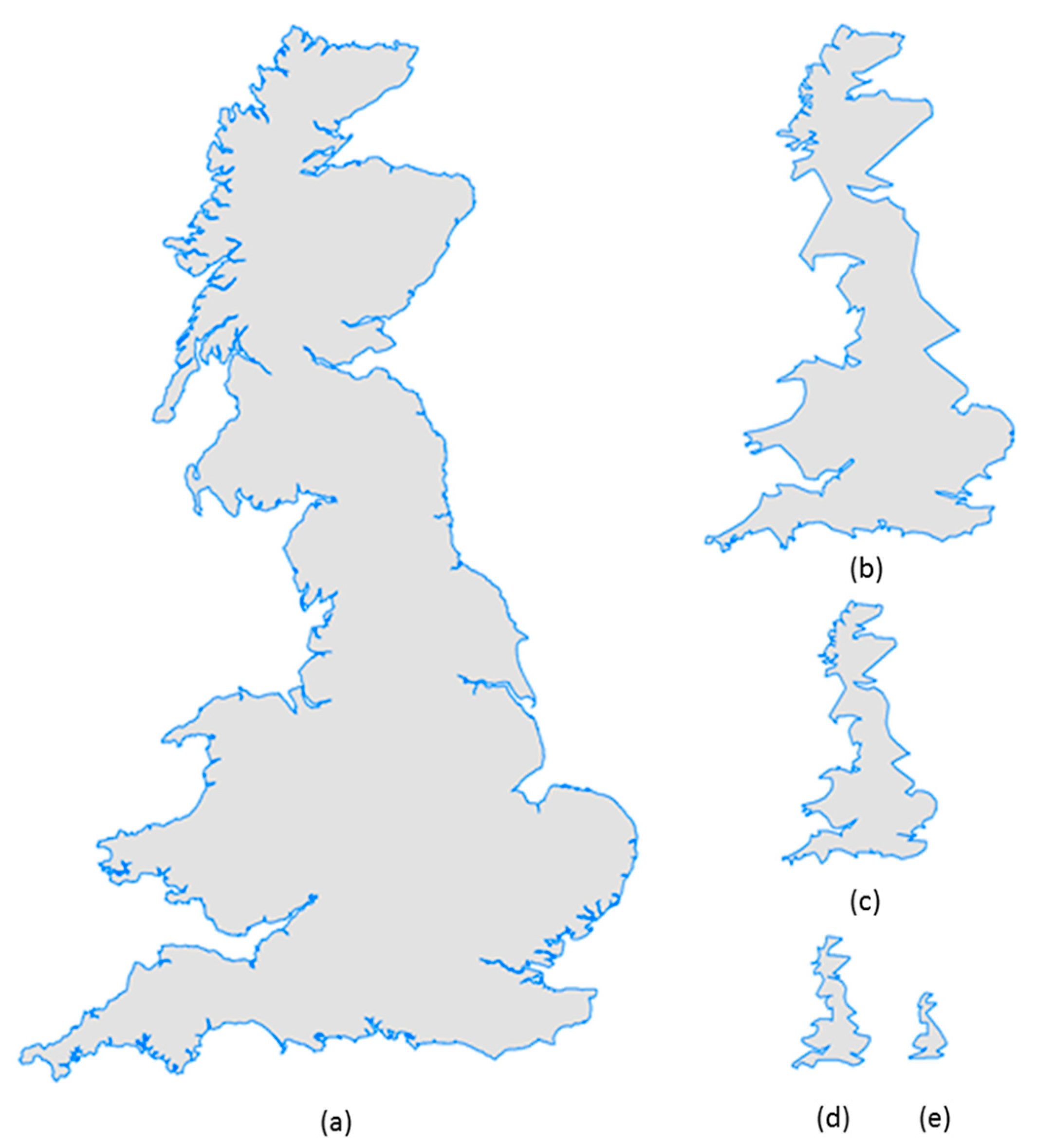
Using the proposed approach, the simplified results can automatically serve as a multiscale representation because each level of detail can be retained in a smaller scale map recursively. Consider the example of the British coastline that is generalized using the HD method with x; we calculated the scaling ratio of this example using the exponent of x of all convex hulls of the original polygon data. The exponent value was 1.91 so the scaling ratio could be approximately set to 1/2. It should be noted that the idea originated from MapGen [44]. Figure 10 shows the resulting map series, from which we could see that the simplified result at each level fit well with the decrease of scale. In this connection, we further confirm that the fractal-geometric thinking leads us to an objective mapping or map generalization [24], wherein no preset value or threshold is given to control the generalization process. Namely, the generalization of a polygonal feature can be done through its inherent scaling hierarchy, and the scaling ratio of the map series, objectively obtained from the long-tailed distribution of geometric measures (e.g., the power law exponent), can be used to properly map the simplified results. Thus, we believe that the fractal nature of a geographic feature itself provides an effective reference and, more importantly, a new way of thinking and conducting map generalization.
6. Conclusions
Geographic features are inherently fractal. The scaling hierarchy endogenously possessed by a fractal can naturally describe the different levels of details of a shape and can thereby effectively guide the cartographic generalization. In this paper, we implemented PolySimp to derive the scaling hierarchy based on four well-known algorithms: DP, BS, VW, and HD, and conducted the polygon simplification accordingly. We extended the previous study by introducing the predefined three geometric measures of DP to the other three algorithms. As results, the software tool could facilitate the computation of those metrics and use them for obtaining a multiscale representation of a polygonal feature. Apart from the generalization, we found that computed measures could also be used to characterize a polygonal feature as a fractal through its underlying scaling hierarchies. We hope this software tool will showcase the applicability of fractal way of thinking and contribute to the development of map generalization.
Some issues require further research. In this work, although PolySimp can generalize a single polygon into a series of lower level details, the applicability of the tool to multi-polygon simplification, especially for those polygons with a shared boundary, was not considered yet. This will be further improved in order to not only maintain the core shape of a polygon, but also to retain its topology consistency. Moreover, we envisioned only a multiscale representation of a two-dimensional polygon. It would be very promising in future to use PolySimp to compute the scaling hierarchy of a three-dimensional polygon and conduct the cartographic generalization accordingly by applying head/tail breaks.
Supplementary Materials
The executable program and sample data are available online at: https://github.com/dingmartin/PolySimp.
Author Contributions
Conceptualization, Ding Ma; Data curation, Wei Zhu; Formal analysis, Ding Ma and Ye Zheng; Funding acquisition, Ding Ma and Zhigang Zhao; Methodology, Ding Ma and Wei Zhu; Supervision, Renzhong Guo and Zhigang Zhao; Visualization, Wei Zhu; Writing—original draft, Ding Ma; Writing—review & editing, Zhigang Zhao. All authors have read and agreed to the published version of the manuscript.
Funding
This research was funded by the China Postdoctoral Science Foundation [Grant No. 2019M663038], and the Open Fund of the Key Laboratory of Urban Land Resources Monitoring and Simulation, MNR [Grant No. KF-2018-03-036].
Conflicts of Interest
The authors declare no conflict of interest.
Appendix A. The Scaling Hierarchy of Geometric Units Derived from DP, BS, and VW Algorithms
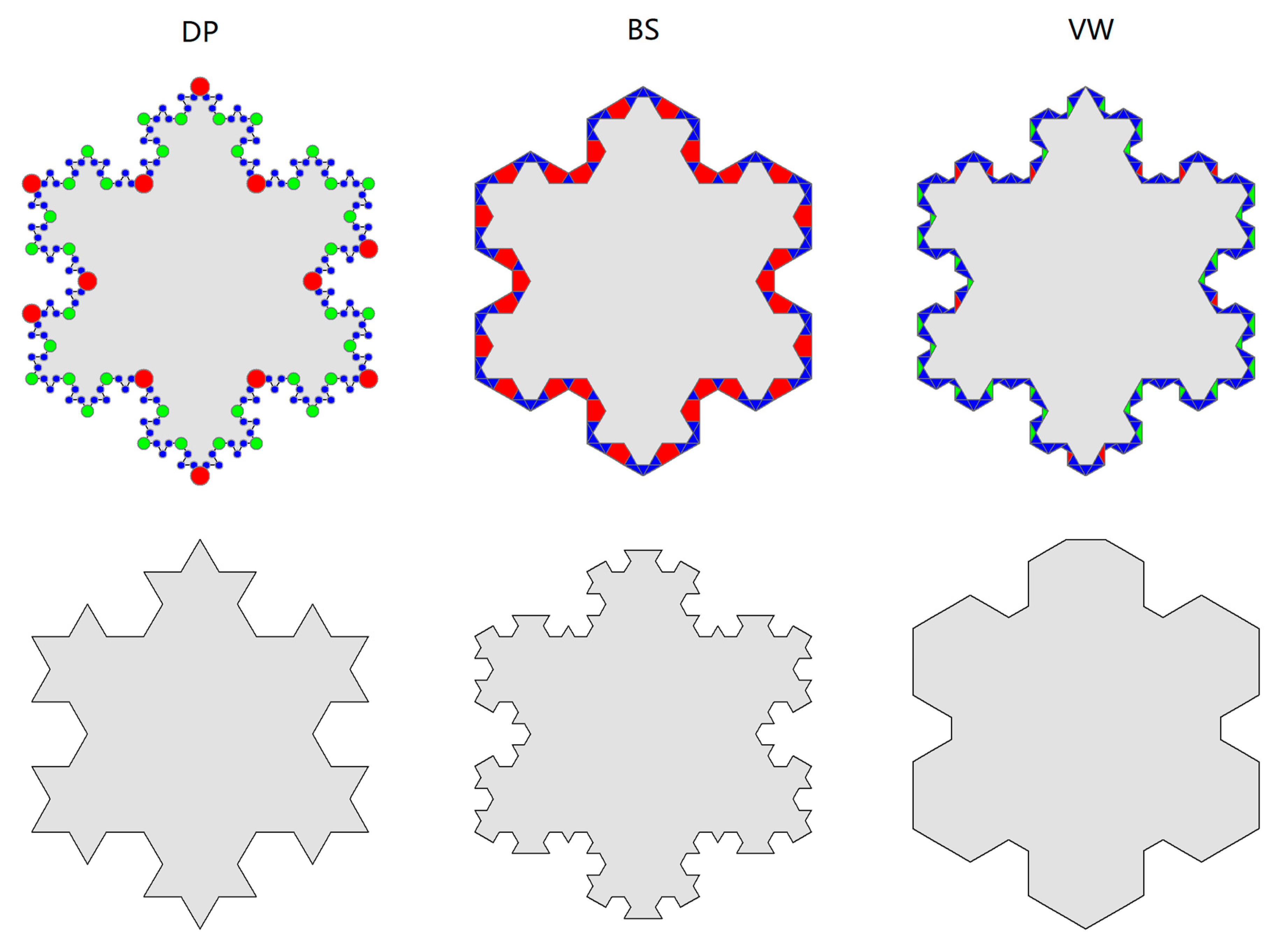
This appendix supplements Section 2.2 by illustrating the scaling pattern of geometric units of a classic fractal—Koch Snowflake. Three types of geometric elements (i.e., characteristic points, bends, and triangles) are derived respectively from DP, BS, and VW methods. Figure A1 shows the scaling hierarchical levels for each type of geometric element with respect to parameter x, wherein the number of levels for DP is three, for BS is two, and for VW is three. Hence, we can spot similar scaling patterns of far more smalls than larges across three methods. Those “larges”—geometric elements in red or green—represent the most essential part and can thus constitute the shape of the snowflake at a coarser level.
Figure A1.
(Color online) The illustration of simplifying geometric units among DP, BS, and VW algorithms using Koch snowflake and the generalization result at the first level. (Note: The size of each type of simplifying units, such as points, triangles, and bends, holds the underlying scaling hierarchy that includes a great many smalls (in blue), a few larges (in red), and some in between (in green), all of which can be used for the guidance of cartographical generalization).

References
- Buttenfield, B.P.; McMaster, R.B. Map Generalization: Making Rules for Knowledge Representation; Longman Group: London, UK, 1991. [Google Scholar]
- Mackaness, W.A.; Ruas, A.; Sarjakoski, L.T. Generalisation of Geographic Information: Cartographic Modelling and Applications; Elsevier: Amsterdam, The Netherlands, 2007. [Google Scholar]
- Stoter, J.; Post, M.; van Altena, V.; Nijhuis, R.; Bruns, B. Fully automated generalization of a 1:50k map from 1:10k data. Cartogr. Geogr. Inf. Sci. 2014, 41, 1–13. [Google Scholar] [CrossRef]
- Burghardt, D.; Duchêne, C.; Mackaness, W. Abstracting Geographic Information in a Data Rich World: Methodologies and Applications of Map Generalisation; Springer: Berlin, Germany, 2014. [Google Scholar]
- Jiang, B.; Liu, X.; Jia, T. Scaling of geographic space as a universal rule for map generalization. Ann. Assoc. Am. Geogr. 2013, 103, 844–855. [Google Scholar] [CrossRef] [Green Version]
- Weibel, R.; Jones, C.B. Computational Perspectives on Map Generalization. GeoInformatica 1998, 2, 307–315. [Google Scholar] [CrossRef]
- McMaster, R.B.; Usery, E.L. A Research Agenda for Geographic Information Science; CRC Press: London, UK, 2005. [Google Scholar]
- Tobler, W.R. Numerical Map Generalization; Department of Geography, University of Michigan: Ann Arbour, MI, USA, 1966. [Google Scholar]
- Li, Z.; Openshaw, S. Algorithms for automated line generalization1 based on a natural principle of objective generalization. Int. J. Geogr. Inf. Syst. 1992, 6, 373–389. [Google Scholar] [CrossRef]
- Visvalingam, M.; Whyatt, J.D. Line generalization by repeated elimination of points. Cartogr. J. 1992, 30, 46–51. [Google Scholar] [CrossRef]
- Saalfeld, A. Topologically consistent line simplification with the Douglas-Peucker algorithm. Cartogr. Geogr. Inf. Sci. 1999, 26, 7–18. [Google Scholar] [CrossRef]
- Gökgöz, T.; Sen, A.; Memduhoglu, A.; Hacar, M. A new algorithm for cartographic simplification of streams and lakes using deviation angles and error bands. ISPRS Int. J. Geo-Inf. 2015, 4, 2185–2204. [Google Scholar] [CrossRef] [Green Version]
- Kolanowski, B.; Augustyniak, J.; Latos, D. Cartographic Line Generalization Based on Radius of Curvature Analysis. ISPRS Int. J. Geo-Inf. 2018, 7, 477. [Google Scholar] [CrossRef] [Green Version]
- Ruas, A. Modèle de Généralisation de Données Géographiques à Base de Contraintes et D’autonomie. Ph.D. Thesis, Université Marne La Vallée, Marne La Vallée, France, 1999. [Google Scholar]
- Touya, G.; Duchêne, C.; Taillandier, P.; Gaffuri, J.; Ruas, A.; Renard, J. Multi-Agents Systems for Cartographic Generalization: Feedback from Past and On-going Research. Technical Report; LaSTIG, équipe COGIT. hal-01682131; IGN (Institut National de l’Information Géographique et Forestière): Saint-Mandé, France, 2018; Available online: https://hal.archives-ouvertes.fr/hal-01682131/document (accessed on 6 October 2020).
- Harrie, L.; Sarjakoski, T. Simultaneous Graphic Generalization of Vector Data Sets. GeoInformatica 2002, 6, 233–261. [Google Scholar] [CrossRef]
- Zahn, C.T.; Roskies, R.Z. Fourier descriptors for plane closed curves. IEEE Trans. Comput. 1972, C-21, 269–281. [Google Scholar] [CrossRef]
- Mandelbrot, B. The Fractal Geometry of Nature; W. H. Freeman and Co.: New York, NY, USA, 1982. [Google Scholar]
- Normant, F.; Tricot, C. Fractal simplification of lines using convex hulls. Geogr. Anal. 1993, 25, 118–129. [Google Scholar] [CrossRef]
- Lam, N.S.N. Fractals and scale in environmental assessment and monitoring. In Scale and Geographic Inquiry; Sheppard, E., McMaster, R.B., Eds.; Blackwell Publishing: Oxford, UK, 2004; pp. 23–40. [Google Scholar]
- Batty, M.; Longley, P.; Fotheringham, S. Urban growth and form: Scaling, fractal geometry, and diffusion-limited aggregation. Environ. Plan. A Econ. Space 1989, 21, 1447–1472. [Google Scholar] [CrossRef]
- Batty, M.; Longley, P. Fractal Cities: A Geometry of Form and Function; Academic Press: London, UK, 1994. [Google Scholar]
- Bettencourt, L.M.A.; Lobo, J.; Helbing, D.; Kühnert, C.; West, G.B. Growth, innovation, scaling, and the pace of life in cities. Proc. Natl. Acad. Sci. USA 2007, 104, 7301–7306. [Google Scholar] [CrossRef] [PubMed] [Green Version]
- Jiang, B. The fractal nature of maps and mapping. Int. J. Geogr. Inf. Sci. 2015, 29, 159–174. [Google Scholar] [CrossRef] [Green Version]
- Töpfer, F.; Pillewizer, W. The principles of selection. Cartogr. J. 1966, 3, 10–16. [Google Scholar] [CrossRef]
- Jiang, B. Head/tail breaks: A new classification scheme for data with a heavy-tailed distribution. Prof. Geogr. 2013, 65, 482–494. [Google Scholar] [CrossRef]
- Jiang, B.; Yin, J. Ht-index for quantifying the fractal or scaling structure of geographic features. Ann. Assoc. Am. Geogr. 2014, 104, 530–541. [Google Scholar] [CrossRef]
- Long, Y.; Shen, Y.; Jin, X.B. Mapping block-level urban areas for all Chinese cities. Ann. Am. Assoc. Geogr. 2016, 106, 96–113. [Google Scholar] [CrossRef] [Green Version]
- Long, Y. Redefining Chinese city system with emerging new data. Appl. Geogr. 2016, 75, 36–48. [Google Scholar] [CrossRef]
- Gao, P.C.; Liu, Z.; Xie, M.H.; Tian, K.; Liu, G. CRG index: A more sensitive ht-index for enabling dynamic views of geographic features. Prof. Geogr. 2016, 68, 533–545. [Google Scholar] [CrossRef]
- Gao, P.C.; Liu, Z.; Tian, K.; Liu, G. Characterizing traffic conditions from the perspective of spatial-temporal heterogeneity. ISPRS Int. J. Geo-Inf. 2016, 5, 34. [Google Scholar] [CrossRef] [Green Version]
- Liu, P.; Xiao, T.; Xiao, J.; Ai, T. A multi-scale representation model of polyline based on head/tail breaks. Int. J. Geogr. Inf. Sci. 2020. [Google Scholar] [CrossRef]
- Müller, J.C.; Lagrange, J.P.; Weibel, R. GIS and Generalization: Methodology and Practice; Taylor & Francis: London, UK, 1995. [Google Scholar]
- Li, Z. Algorithmic Foundation of Multi-Scale Spatial Representation; CRC Press: London, UK, 2007. [Google Scholar]
- ESRI. How Simplify Line and Simplify Polygon Work. Available online: https://desktop.arcgis.com/en/arcmap/latest/tools/cartography-toolbox/simplify-polygon.htm (accessed on 15 July 2020).
- Touya, G.; Lokhat, I.; Duchêne, C. CartAGen: An Open Source Research Platform for Map Generalization. In Proceedings of the International Cartographic Conference 2019, Tokyo, Japan, 15–20 July 2019; pp. 1–9. [Google Scholar]
- CartAGen. Line Simplification Algorithms. 2020. Available online: https://ignf.github.io/CartAGen/docs/algorithms.html (accessed on 6 October 2020).
- Douglas, D.; Peucker, T. Algorithms for the reduction of the number of points required to represent a digitized line or its caricature. Can. Cartogr. 1973, 10, 112–122. [Google Scholar] [CrossRef] [Green Version]
- Zhou, S.; Christopher, B.J. Shape-Aware Line Generalisation with Weighted Effective Area. In Developments in Spatial DataHandling, Proceedings of the 11th International Symposium on Spatial Handling, Zurich, Switzerland; Fisher, P.F., Ed.; Springer-Verlag: Berlin/Heidelberg, Germany, 2005; pp. 369–380. [Google Scholar]
- Wang, Z.; Müller, J.C. Line Generalization Based on Analysis of Shape Characteristics. Cartog. Geogr. Inf. Syst. 1998, 25, 3–15. [Google Scholar] [CrossRef]
- Ai, T.; Li, Z.; Liu, Y. Progressive transmission of vector data based on changes accumulation model. In Developments in Spatial Data Handling; Springer-Verlag: Heidelberg, Germany, 2005; pp. 85–96. [Google Scholar]
- Ma, D.; Jiang, B. A smooth curve as a fractal under the third definition. Cartographica 2018, 53, 203–210. [Google Scholar] [CrossRef] [Green Version]
- Sester, M.; Brenner, C. A vocabulary for a multiscale process description for fast transmission and continuous visualization of spatial data. Comput. Geosci. 2009, 35, 2177–2184. [Google Scholar] [CrossRef]
- Jiang, B. Methods, Apparatus and Computer Program for Automatically Deriving Small-Scale Maps. U.S. Patent WO 2018/116134, PCT/IB2017/058073, 28 June 2018. [Google Scholar]
Figure 1.
(Color online) The simplification process of the Koch snowflake guided by head/tail breaks. (Note: The blue polygons in each panel denote the head parts, whereas the red triangles represent the tail part, which needed to be eliminated progressively for generalization purpose).
Figure 1.
(Color online) The simplification process of the Koch snowflake guided by head/tail breaks. (Note: The blue polygons in each panel denote the head parts, whereas the red triangles represent the tail part, which needed to be eliminated progressively for generalization purpose).

Figure 2.
(Color online) Illustration of geometric measures for the (a) point-based simplifying unit (e.g., Douglas–Peucker (DP) algorithm) and (b) areal-based unit (e.g., bend simplify (BS) and hierarchical decomposition of a polygon (HD) algorithm).
Figure 2.
(Color online) Illustration of geometric measures for the (a) point-based simplifying unit (e.g., Douglas–Peucker (DP) algorithm) and (b) areal-based unit (e.g., bend simplify (BS) and hierarchical decomposition of a polygon (HD) algorithm).
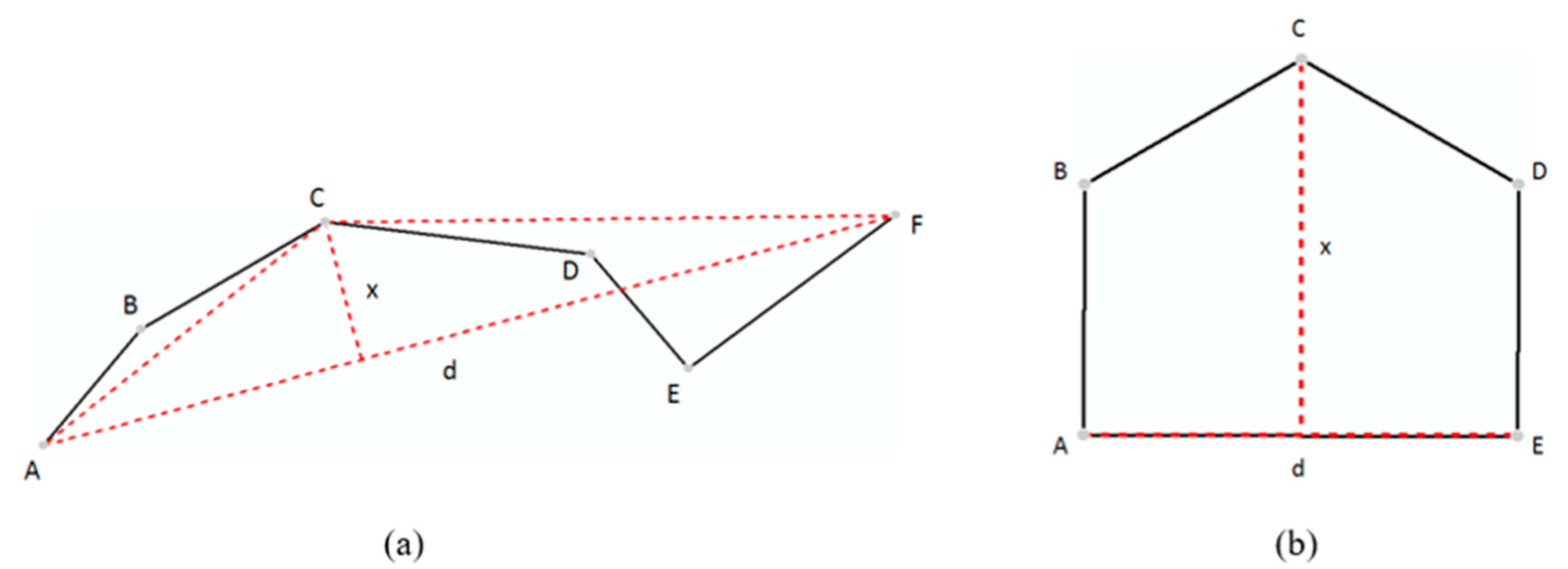
Figure 3.
(Color online) Illustration of the HD algorithm using the Koch snowflake as a working example. Note that the size of derived convex hulls holds a striking scaling hierarchy of far more small ones than large ones.
Figure 3.
(Color online) Illustration of the HD algorithm using the Koch snowflake as a working example. Note that the size of derived convex hulls holds a striking scaling hierarchy of far more small ones than large ones.
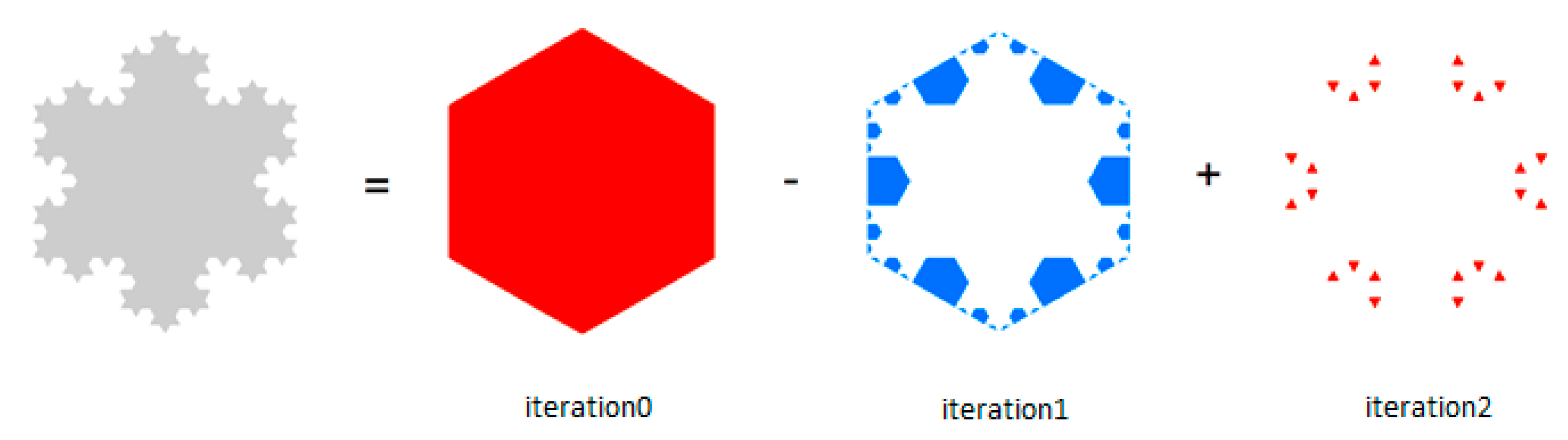
Figure 4.
The tool for easily conducting cartographical simplification of polygonal features based on its inherent scaling hierarchies.
Figure 4.
The tool for easily conducting cartographical simplification of polygonal features based on its inherent scaling hierarchies.
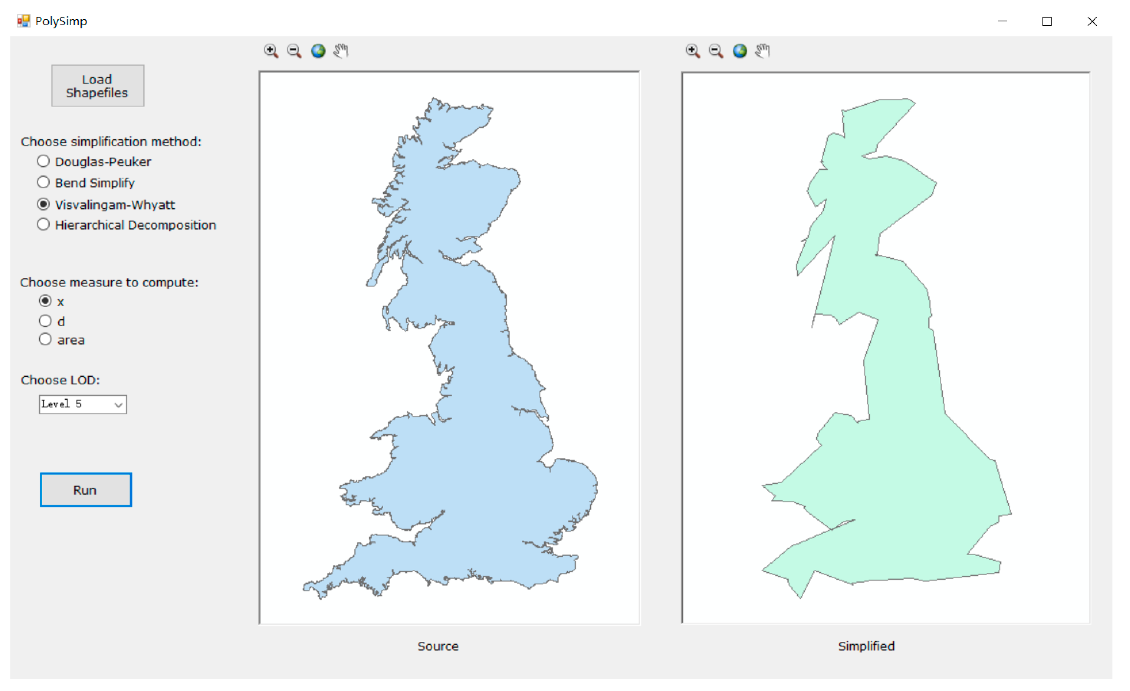
Figure 5.
Flow chart for conducting polygon simplification based on head/tail breaks for each algorithm.
Figure 5.
Flow chart for conducting polygon simplification based on head/tail breaks for each algorithm.
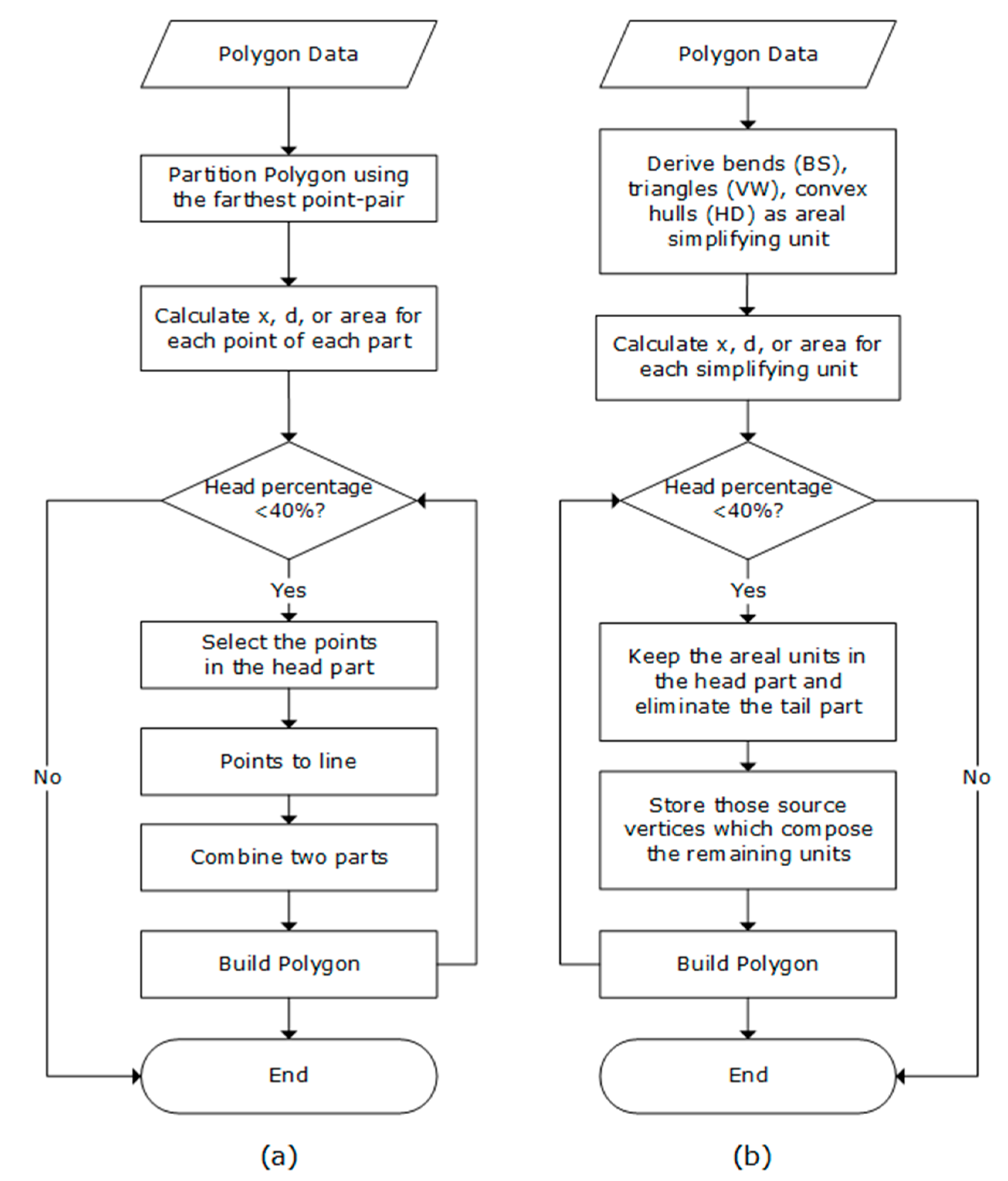
Figure 6.
(Color online) Basic geometric units of a part of the British coastline (referring to the red box in the right panel) for each polygon simplification algorithm derived by PolySimp. (Note: Panels on the left show a clear scaling hierarchy of far more small ones than large ones, represented by either dot size or patch color).

Figure 7.
(Color online) The simplified results of the British coastline at different levels of details through four algorithms in terms of the polygonal shape based on x (a), d (b), and area (c); and the corresponding number of points (d) respectively.
Figure 7.
(Color online) The simplified results of the British coastline at different levels of details through four algorithms in terms of the polygonal shape based on x (a), d (b), and area (c); and the corresponding number of points (d) respectively.
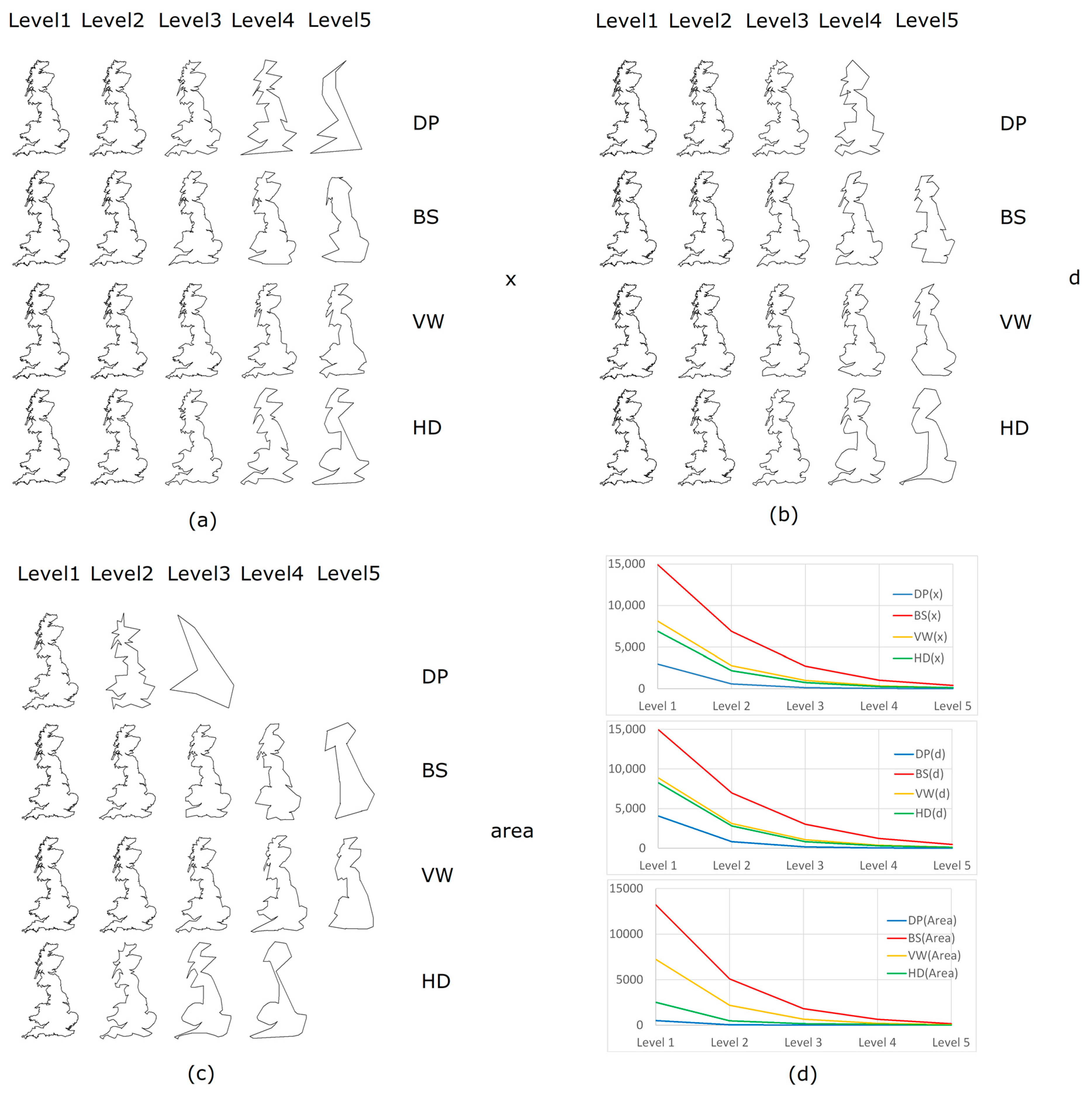
Figure 8.
(Color Online) The shape variation of simplified results of the British coastline at five levels of details, indicated by the polygon’s area (Panels a–c), perimeter (Panels e–g), and shape factor (Panels h–j).
Figure 8.
(Color Online) The shape variation of simplified results of the British coastline at five levels of details, indicated by the polygon’s area (Panels a–c), perimeter (Panels e–g), and shape factor (Panels h–j).
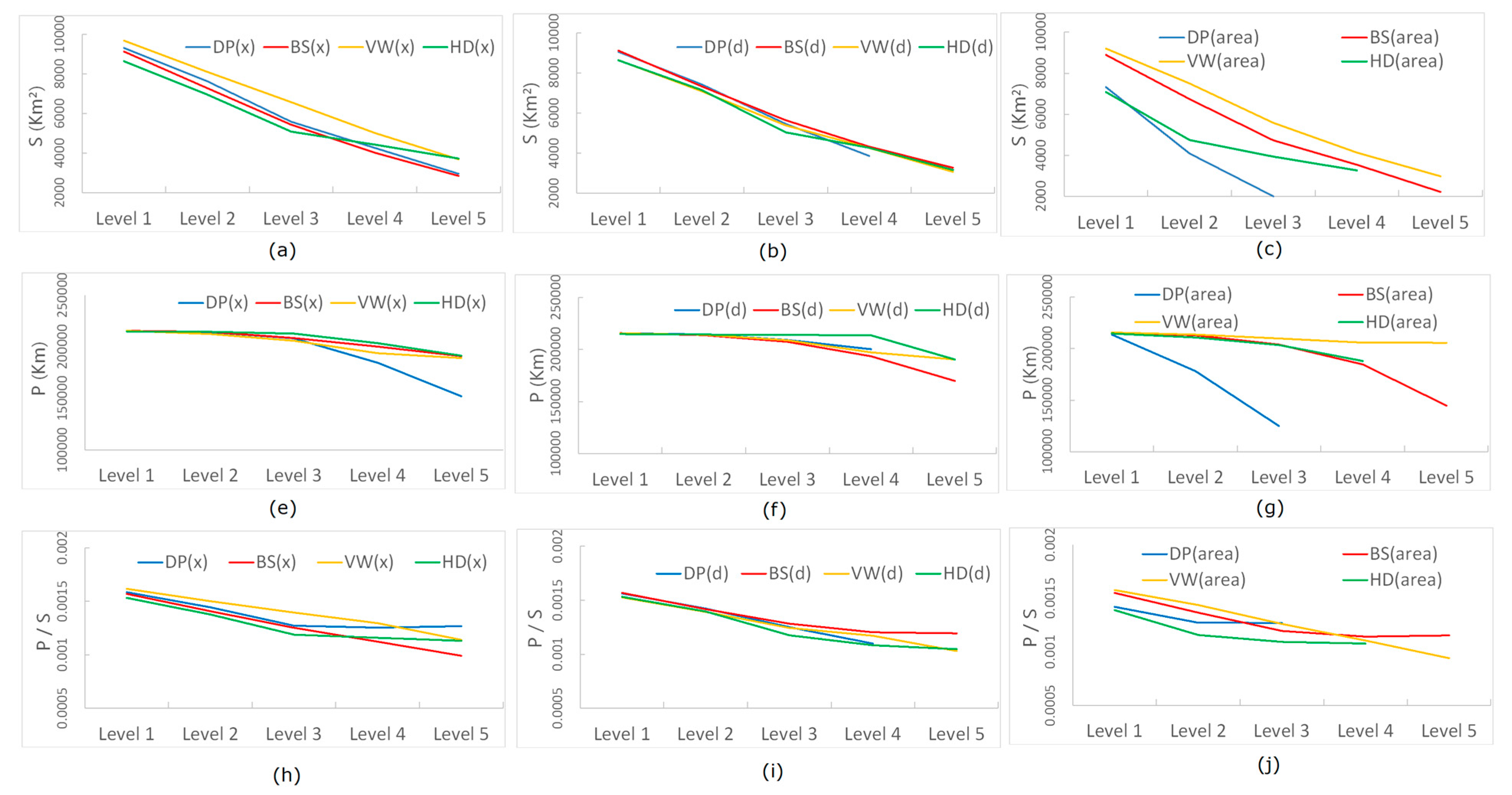
Figure 9.
(Color online) The first iteration of the simplification process of the Koch snowflake guided by area (note: Red triangles are the tail part that needs to be eliminated at the first level).
Figure 9.
(Color online) The first iteration of the simplification process of the Koch snowflake guided by area (note: Red triangles are the tail part that needs to be eliminated at the first level).

Figure 10.
(Color online) A multiscale representation with the scaling ratio of 1/2 of the simplified result from level 1 to 5 (Panels a–e) of the British coastline using the HD algorithm.
Figure 10.
(Color online) A multiscale representation with the scaling ratio of 1/2 of the simplified result from level 1 to 5 (Panels a–e) of the British coastline using the HD algorithm.

Table 1.
Average running times (in seconds) required to simplify the British coastline at a single level by different methods using PolySimp. (Note: Configurations of computer used to perform experiments. Operating system: Windows 10 x64; CPU: Intel® CoreTM i7-9700U @ 3.60 GHz; RAM: 16.00 GB).
Table 1.
Average running times (in seconds) required to simplify the British coastline at a single level by different methods using PolySimp. (Note: Configurations of computer used to perform experiments. Operating system: Windows 10 x64; CPU: Intel® CoreTM i7-9700U @ 3.60 GHz; RAM: 16.00 GB).
| DP | BS | VW | HD | |
|---|---|---|---|---|
| Time (x) | 1.06 | 4.32 | 0.25 | 103.92 |
| Time (d) | 1.12 | 4.43 | 0.19 | 75.67 |
| Time(area) | 1.08 | 4.31 | 0.24 | 34.83 |
Table 2.
Ht-index of three parameters for each algorithm on the source data of the British coastline. (Note: 40% as threshold for the head/tail breaks process).
Table 2.
Ht-index of three parameters for each algorithm on the source data of the British coastline. (Note: 40% as threshold for the head/tail breaks process).
| DP | BS | VW | HD | |
|---|---|---|---|---|
| Ht (x) | 6 | 9 | 10 | 6 |
| Ht (d) | 5 | 6 | 8 | 7 |
| Ht (area) | 4 | 6 | 7 | 5 |
Table 3.
Point numbers at the top 5 levels according to parameters x, d, and area through DP, BS, VW, and HD algorithms, respectively (Note: # = number, NA = not available).
Table 3.
Point numbers at the top 5 levels according to parameters x, d, and area through DP, BS, VW, and HD algorithms, respectively (Note: # = number, NA = not available).
| Level 1 | Level 2 | Level 3 | Level 4 | Level 5 | |
|---|---|---|---|---|---|
| #Pt(x)-DP | 2969 | 583 | 133 | 34 | 12 |
| #Pt(d)-DP | 4074 | 829 | 173 | 45 | NA |
| #Pt(area)-DP | 505 | 48 | 10 | NA | NA |
| #Pt(x)-BS | 14,913 | 6883 | 2706 | 1023 | 395 |
| #Pt(d)-BS | 14,957 | 6970 | 3037 | 1238 | 485 |
| #Pt(area)-BS | 13,234 | 5086 | 1816 | 638 | 159 |
| #Pt(x)-VW | 8112 | 2762 | 990 | 346 | 119 |
| #Pt(d)-VW | 8866 | 3124 | 1078 | 378 | 124 |
| #Pt(area)-VW | 7233 | 2178 | 661 | 192 | 62 |
| #Pt(x)-HD | 6899 | 2162 | 743 | 260 | 127 |
| #Pt(d)-HD | 8262 | 2814 | 827 | 311 | 112 |
| #Pt(area)-HD | 2509 | 483 | 159 | 91 | NA |
© 2020 by the authors. Licensee MDPI, Basel, Switzerland. This article is an open access article distributed under the terms and conditions of the Creative Commons Attribution (CC BY) license (http://creativecommons.org/licenses/by/4.0/).
Share and Cite
MDPI and ACS Style
Ma, D.; Zhao, Z.; Zheng, Y.; Guo, R.; Zhu, W. PolySimp: A Tool for Polygon Simplification Based on the Underlying Scaling Hierarchy. ISPRS Int. J. Geo-Inf. 2020, 9, 594. https://0-doi-org.brum.beds.ac.uk/10.3390/ijgi9100594
AMA Style
Ma D, Zhao Z, Zheng Y, Guo R, Zhu W. PolySimp: A Tool for Polygon Simplification Based on the Underlying Scaling Hierarchy. ISPRS International Journal of Geo-Information. 2020; 9(10):594. https://0-doi-org.brum.beds.ac.uk/10.3390/ijgi9100594
Chicago/Turabian StyleMa, Ding, Zhigang Zhao, Ye Zheng, Renzhong Guo, and Wei Zhu. 2020. "PolySimp: A Tool for Polygon Simplification Based on the Underlying Scaling Hierarchy" ISPRS International Journal of Geo-Information 9, no. 10: 594. https://0-doi-org.brum.beds.ac.uk/10.3390/ijgi9100594
Note that from the first issue of 2016, this journal uses article numbers instead of page numbers. See further details here.