Article

Hierarchical Instance Recognition of Individual Roadside Trees in Environmentally Complex Urban Areas from UAV Laser Scanning Point Clouds

1
Key Laboratory of Virtual Geographic Environment, Ministry of Education, Nanjing Normal University, Nanjing 210093, China
2
Jiangsu Center for Collaborative Innovation in Geographical Information Resource Development and Application, Nanjing 210023, China
3
State Key Laboratory Cultivation Base of Geographical Environment Evolution, Nanjing Normal University, Nanjing 210093, China
4
Key Laboratory of Urban Land Resources Monitoring and Simulation, Ministry of Natural Resources, Shenzhen 518034, China
5
State Key Laboratory of Information Engineering in Surveying, Mapping, and Remote Sensing, Wuhan University, Wuhan 430072, China
*
Author to whom correspondence should be addressed.
ISPRS Int. J. Geo-Inf. 2020, 9(10), 595; https://0-doi-org.brum.beds.ac.uk/10.3390/ijgi9100595
Submission received: 7 September 2020 / Revised: 27 September 2020 / Accepted: 4 October 2020 / Published: 10 October 2020
(This article belongs to the Special Issue Advanced Research Based on Multi-Dimensional Point Cloud Analysis)

Abstract

:
Individual tree segmentation is essential for many applications in city management and urban ecology. Light Detection and Ranging (LiDAR) system acquires accurate point clouds in a fast and environmentally-friendly manner, which enables single tree detection. However, the large number of object categories and occlusion from nearby objects in complex environment pose great challenges in urban tree inventory, resulting in omission or commission errors. Therefore, this paper addresses these challenges and increases the accuracy of individual tree segmentation by proposing an automated method for instance recognition urban roadside trees. The proposed algorithm was implemented of unmanned aerial vehicles laser scanning (UAV-LS) data. First, an improved filtering algorithm was developed to identify ground and non-ground points. Second, we extracted tree-like objects via labeling on non-ground points using a deep learning model with a few smaller modifications. Unlike only concentrating on the global features in previous method, the proposed method revises a pointwise semantic learning network to capture both the global and local information at multiple scales, significantly avoiding the information loss in local neighborhoods and reducing useless convolutional computations. Afterwards, the semantic representation is fed into a graph-structured optimization model, which obtains globally optimal classification results by constructing a weighted indirect graph and solving the optimization problem with graph-cuts. The segmented tree points were extracted and consolidated through a series of operations, and they were finally recognized by combining graph embedding learning with a structure-aware loss function and a supervoxel-based normalized cut segmentation method. Experimental results on two public datasets demonstrated that our framework achieved better performance in terms of classification accuracy and recognition ratio of tree.

1. Introduction

According to research of the United Nations Commission on Sustainable Development (CSD), around 70% of the world’s population is expected to live in cities by 2050 [1]. Rapid urbanization may cause a series of urban environmental problems that humanity urgently needs to face, such as global warming, poor air quality, urban floods, urban heat island effect, and noise [2]. Urban trees provide people with a beautiful and comfortable living environment, which can alleviate various environmental problems mentioned above. As a significant requirement of smart cities, roadside trees inventory is crucial in urban environmental construction. However, urban trees inventories in many cities are regularly inaccurate and incomplete due to financial problems. According to a survey conducted by the United Nations Board of Auditors (UNBoA), less than 20% of the cities in the United States have information on urban tree inventories, only a few European countries have management plans for urban forests, and many of Chinese cities lack the strategies and funding for urban tree inventories [3]. Consequently, it is imminent to carry out research related to urban trees inventories.
Extraction and segmentation of roadside trees is the basis of urban tree inventories and plays a key role in various applications, including distribution of urban trees, carbon storage capacity of trees, and post-disaster damage. The isolated trees can be utilized to explore urban microclimate and loss of trees after a typhoon; thereby providing comprehensive and accurate information for urban tree planting and management. With the rapid development of technology, traditional methods of manually measuring trees have gradually been replaced by machine measurements. Besides, images-based methods for the urban tree inventory face plenty of challenges including the limited image resolution, sensitivity to weather conditions, and difficulties of geo-registration. Recently, the rapid development of LiDAR technology makes it possible to acquire massive 3D geospatial information for the trees in urban scenes. Research on tree has entered a new era [4,5].
As we all know, forest inventory (the same goes for urban tree inventory) requires accurate individual tree structural attributes. Thus, the instance segmentation of roadside trees is the important part of urban green space management. Numerous research methods focused on trees recognition have been developed in recent years. To fully take advantages of the well-developed image-processing algorithms in tree crowns delineation, the height variation of canopy height model (CHM) is employed to find treetops. According to the statement of [6], the CHM-based tree detection algorithms (such as watershed analysis [7], spatial wavelet analysis [8], and template matching [9]) are fast and efficient but the existing problems are also obvious: it changes the shape of the tree crown to a certain extent, reducing the original data information thanks to a variety of canopy sizes.
Some studies directly segmented individual trees on original point clouds since the increased spatial resolution of ALS (airborne laser scanning) point cloud. A portion of existing point-based clustering methods [10,11,12,13,14] have been widely used for individual tree segmentation. Compared with CHM-based methods, point-based clustering methods prove to be robust to various types of trees and greatly improve computational efficiency and require no prior knowledge of the shapes and sizes of tree crowns. Nevertheless, for the above methods directly work on LiDAR data, there are three unavoidable problems: (1) serious omission errors caused by the complexity of urban areas (such as the spatial heterogeneity of urban forests) [15]; (2) commission errors caused by the diverse structure and irregular shape of urban trees [16]; (3) suppressed trees (which have less information) and small trees (which are blended with or located below tall trees) are difficult extracted and segmented due to mobile laser scanning systems hard to penetrate the dense forest canopy [17].
Urban regions are a mosaic of kinds of objects, which will lower the efficiency and feasibility of LiDAR data processing [18]. Thus, compared with the ALS point cloud, mobile laser scanning (MLS) and terrestrial laser scanning (TLS) data are used less in urban trees inventory. In this paper, the data acquired by UAV-based mobile LiDAR system is applied to detect and segment individual trees, aiming at automated urban roadside tree inventory. Our work is divided into two parts: tree-like objects extraction based on the point cloud labeling using pointwise semantic learning network, and individual roadside trees recognition based on a novel graph convolutional neural network.
Urban roadside trees extraction and recognition is a long-standing, yet still active topic. The research on roadside trees from point cloud in urban areas is relatively less than that of forestry resource inventory. In addition, the LiDAR data collected in the forest area mainly consist of tree, while the urban scene contains various artifacts, which increases the complexity of tree segmentation task. As regard to trees extraction, existing work can be further divided into two types: geometric rule-based and semantic labeling-based methods.
Geometric rule-based methods generally detect and extract trees from environmentally complex scenes using geometric attributes [19] such as tree shape, cylindrical trunk shape, points distribution, etc. They can be divided into three classes: the clustering [20], region growing [21], and density threshold-based method [22]. All of the above methods performed well in their own research areas. However, they are basically difficult to extract trees from large-scale scenes of dense mixed objects in urban areas, because the heavy computing costs required for local geometric features. Specifically, most rule-based works are traditional and not competitive in speed and accuracy.
In recent years, a series of deep learning methods are tried to apply to 3D semantic segmentation [23]. Note that deep learning based semantic segmentation of point clouds in outdoor scenes often includes category of trees, this work is beneficial to complete the task of tree segmentation from laser scanning data. The most direct way to exploit deep learning on the LiDAR point cloud classification is to first convert the 3D points to regular collections of 2D images in various ways. Semantic segmentation is then performed through a mature deep neural network (DNN) in the image field, and finally transfer the image segmentation result back to the point cloud [24,25,26]. However, these models cause spatial information loss and induce quantization errors in the conversion process [27]. Another feasible method is to extend 2D convolution to 3D convolutional neural network (3D CNN). Most researchers develop the professional model to transform point clouds to 3D voxels, followed by a 3D CNN that predicts the semantic label based on the occupancy grid [28]. However, 3D volumetric grids entail substantial memory consumption and computational cost.
To overcome the shortcomings of the above two methods, some work directly employs deep learning models on raw point clouds. However, CNNs can handle only regular input format. Direct application of standard CNNs to unordered and unstructured point clouds is infeasible. In terms of this, the pioneering work PointNet [29] propose to learn per-point features using shared multi-layer perceptron (MLP) and global features using symmetrical pooling functions. Based on PointNet, a series of point-based networks have been proposed recently [23]. Overall, these methods can be roughly divided into pointwise MLP methods [30,31,32,33], point convolution methods [34,35,36,37], RNN (Recurrent Neural Network)-based methods [38,39,40,41], and graph-based methods [42,43,44,45]. To summarize, most of the existing deep learning-related methods that only focus on either global or local statistical information, result in a performance reduction in representativeness and descriptiveness. In addition, some of above models employ standard convolution kernels with regular receptive fields, which neglect the structural connections between points and fail to account for varying point density.
Our method follows an idea similar to the point convolution methods, however, instead of only focusing on the single features and ignore other relationships between individual points in PointNet-derived deep learning models, we propose a point-wise semantic learning network to acquire both global and local information of each point, avoiding the information loss in local neighborhoods and reducing useless convolutional computations.
To improve the segmentation accuracy and efficiency simultaneously, we propose a deep learning approach designed for recognizing individual trees from UAV-LS data. The non-ground points are identified and acquired; subsequently, a revised point-wise convolution algorithm is proposed to extract trees from non-ground points firstly; a graph-structured optimization algorithm is then performed to obtain optimal classification results; finally, a novel approach called 3D graph embedding learning with a structure-aware loss function is introduced for individual roadside trees segmentation. To the best of our knowledge, this paper is the earlier application of deep learning based instance segmentation method [46] to segment individual trees from ALS point clouds. We aim to obtain satisfactory segmentation results by utilizing deep learning while substantially reducing the impact of scene complexity.
The main contributions of our approach include the following three aspects:
(i) Presentation of the urban scene understanding and the approach of roadside tree recognition from the input of the UAV-LS data to the tree segmentation.
(ii) Improved classification of large-scale 3D unordered points without voxelizing by using pointwise semantic learning network. Most of the parameters in the network are learned, and thus the intensive parameter tuning cost is significantly reduced.
(iii) Effective aggregation of multi-level information (geometric information, discriminative embedding information, and information from neighbors) and elimination of quantization errors caused by regular voxelization by using graph convolutional neural network combining structure-aware loss function with the attention-based k-nearest neighbor.

2. Materials and Methods

As shown in Figure 1, our method consists of four main steps: (1) Ground removal (2.1). Raw data is divided into ground and non-ground points by an improved filtering algorithm. (2) Roadside trees objects detection (2.2). Roadside trees objects are obtained through deep learning approaches based on the revised PointNet network on non-ground points. (3) Labeling refinement (2.3). A graph-structured optimization algorithm is performed to achieve spatial smoothing of the initial semantic labeling results. (4) Recognition of individual roadside trees (2.4). Roadside trees objects are segmented by a deep learning based method from point cloud of the given categories. The details of each step of our method are as follows.

2.1. Ground Removal by Improved Progressive TIN Densification Filtering

Because of the scan mode of Aerial LiDAR systems, ground points take up a great portion of the entire scene. Such a great deal of ground points not only enlarge the searching regions for extracting non-ground objects, but also increase the spatial complexities and slow the processing speed. Therefore, removing ground points from a variety of scenes is a preliminary but crucial step. To reduce the quantity of the data to be handled and consider terrain fluctuations in a large scene, we develop an improved progressive triangulated irregular network (TIN) densification (IPTD) filtering algorithm, which can rapidly and effectively distinguish ground points from non-ground points, particularly structurally complex regions.
In existing filtering algorithms, the morphological filtering algorithm [47] obtains non-ground points while retaining the terrain details; the progressive densification method [48] has gained popularity owing to its robustness and effectiveness in segmenting ground points, however, it has inadequacies when dealing with topographically and environmentally complex regions and tends to remove ground points on steep regions and flatten the terrain. To obtain better filtering performance for complex urban areas, we investigate the feasibility of improving progressive TIN densification filtering of point clouds. Compared with previous work [49,50], the enhancements of the proposed IPTD filtering algorithm encompasses three aspects. (1) Potential ground seed points are obtained through extended local minimum for the grids containing points and the nearest neighbor was adopted to interpolate the elevations of grids without points instead of using the lowest points in user-defined grids. (2) Accurate ground seed points are acquired by judging the elevation difference in the neighborhood of the local thin plate spline interpolation by the given threshold. This operation provides more ground seed points that are generally evenly distributed. (3) Before upward densification, downward densification is performed to promote the ability of the proposed algorithm in coping with slope variations. Lastly, the ground points are extracted by iteratively densifying ground seed points, the remaining points are taken as non-ground points. Figure 2 shows an example of the point cloud before and after ground removal, where the colors represent elevation variations.

2.2. Detection of Tree-Like Structures via Pointwise Classification on Non-Ground Points

As a significant requirement of urban tree inventory, labeling input data with the category of tree is fundamental in exploiting the informative values for the instance segmentation of trees. The problem has been extensively researched. Some unified approaches combine handcrafted features in a heuristic manner but fails to capture high-level semantic structures. The segmented points generated by deep-learning methods are often corrupted with noise and outliers due to the unorganized distribution and uneven point density, which are inevitable in complex urban environments. It is a challenge to effectively and automatically recognize individual trees in environmentally complex urban regions from such data. To solve this problem, we revise an existing deep-learning architecture to directly process unstructured point clouds and implement a point-wise semantic learning network.
PointNet has revolutionized how we think about processing point clouds as it offers a learnable structured representation for 3D semantic segmentation tasks. However, the local features of point clouds cannot be effectively robustly learned, limiting its ability to recognize the object of interest in complex scenes. The proposed architecture is similar to PointNet with a few small modifications, i.e., features are computed from local regions instead of the entire point cloud, which makes the estimation of local information more accurate. We propose an improved 3D semantic segmentation network based on pointwise KNN (k-th nearest neighbor) search method, which has unique advantage that extract multi-level features. The proposed network takes local features of a query point from local region composed of neighbors set as its new features and establishes connections between multiple layers by adding skip connections to strengthen the learning ability of local features.
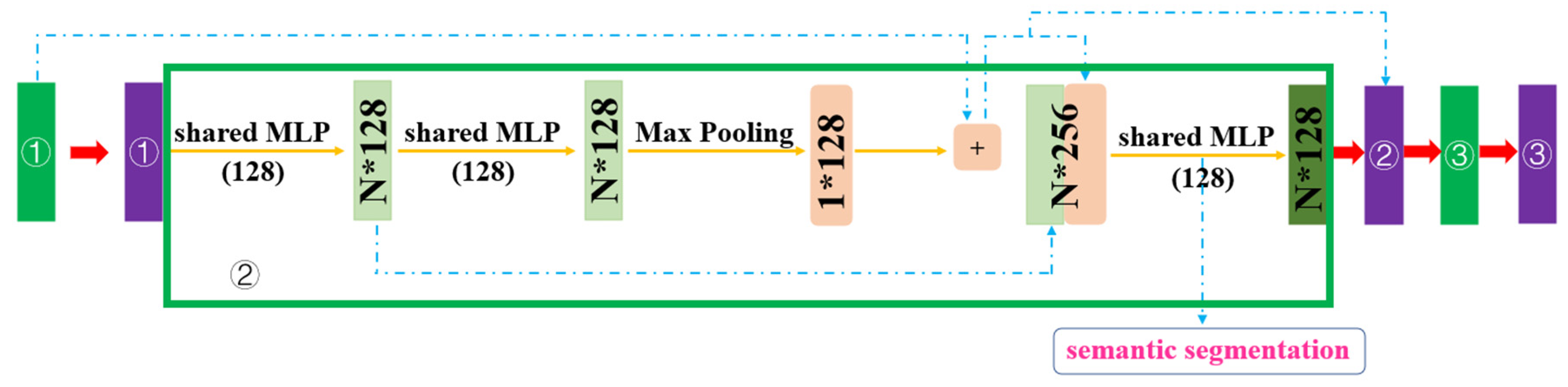
In this section, we further present the theoretical and logical principles of the proposed network for urban object segmentation from non-ground points of ALS data in details. Considering that the descriptiveness of differences between points from low-dimensional initial features is far from satisfactory and the richness of point features is good for local feature extraction, we first enhance the discriminability of point features and then obtain local information in the new feature space. The proposed network mainly contains two modules: (1) implementing optimized PointNet by KNN, which is used to extract more powerful local information in the high-dimensional feature space; (2) semantically segmenting large-scale point cloud using the global and local features. The architecture of the proposed method is summarized in Figure 3.
Our detailed and complete feature learning network is illustrated in 
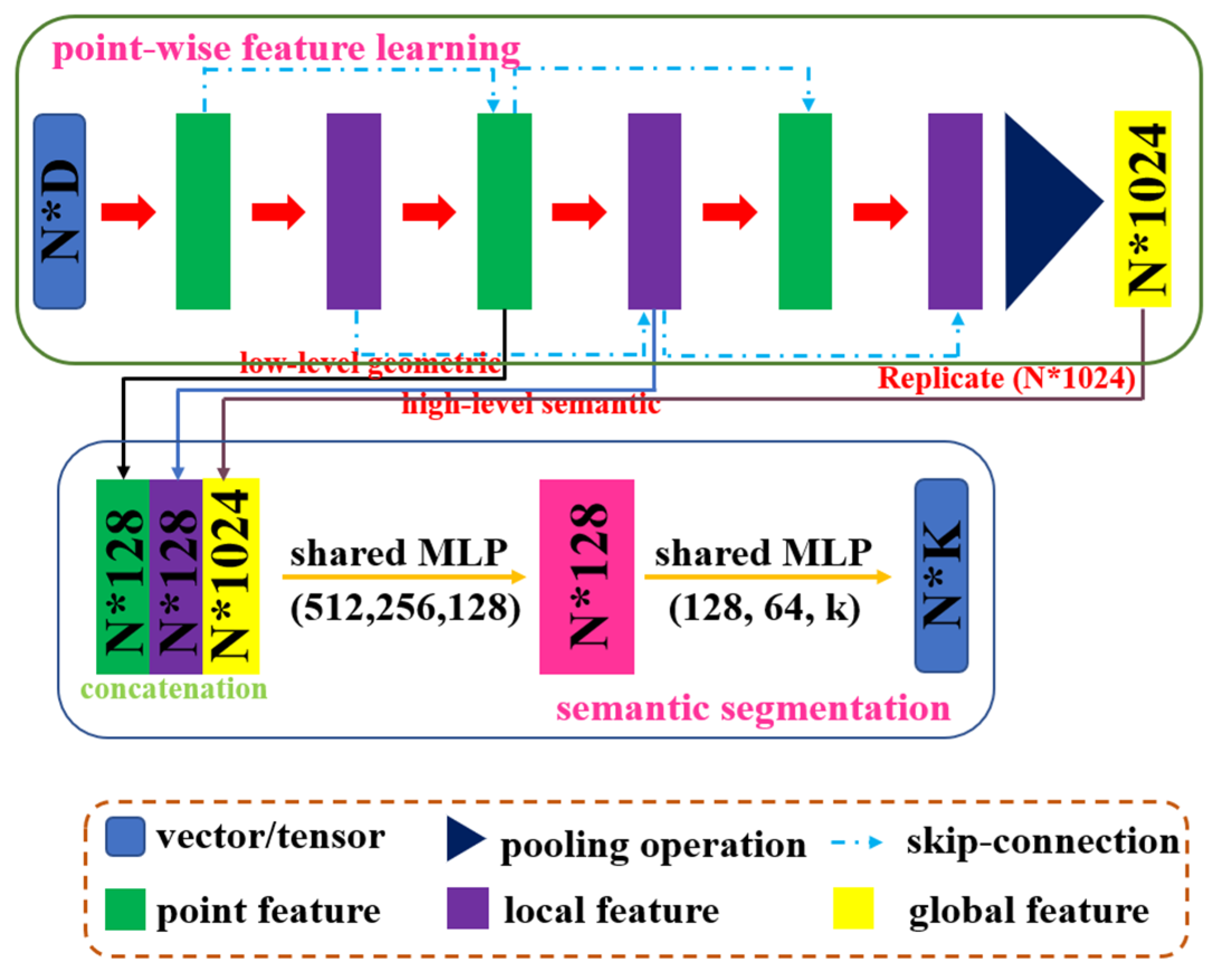
Figure 3, the green part, which consists of two key modules: sub-module of point feature extraction based on PointNet and sub-module of local feature extraction in the high-dimensional feature space.

2.2.1. Sub-Module of Point Feature Extraction

The module is designed to obtain richer point cloud high-dimensional features by using feature extraction operations many times. For the whole pipeline, we directly use simplified PointNet as our backbone network. Our network takes a point cloud of size N × D as input, then encodes it into a N × 128 shaped matrix using the shared Multi-Layer Perceptron (MLP) [29]. After max pooling, the dimension of the global feature of point cloud is 128. Finally, the global features are duplicated N times and concatenates point feature into a feature vector. This vector is then input into the MLP to obtain a novel N × 128 shaped feature vector, which is fed into the following module to acquire the local attributes.
In general, the feature learning network mainly uses three sub-modules of point feature extraction with the same principle. In other words, we perform three repeated feature extractions. We pass and fuse the features of different layers through the connection, for extracting and fusing richer high-level features. The feature learning network illustrated in Figure 4 is composes with two components including a simplified PointNet and connection channels.

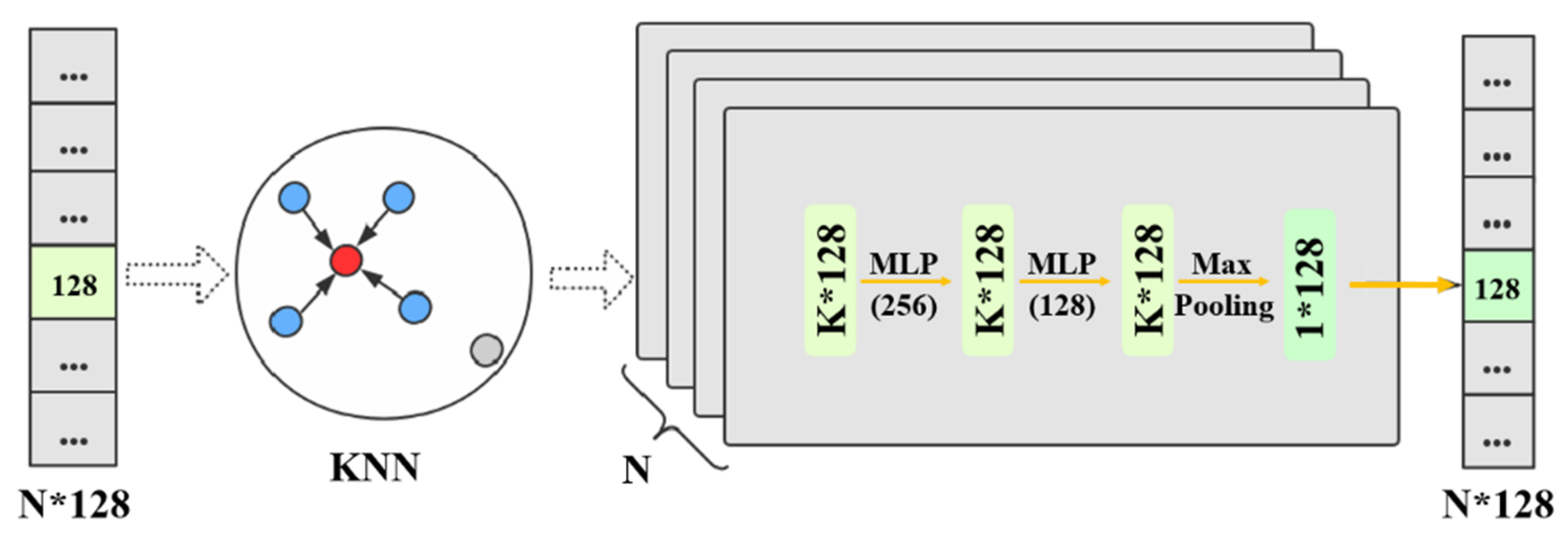
2.2.2. Sub-Module of Local Feature Extraction

The features of points belonging to the same semantic category are similar, this module aims to reduce the feature distance between similar points and increase the discriminability of different point clouds. The output from the above module forms a N × 128 tensor with low-level information. To get sufficient expressive power to transform each point feature into a higher-dimensional feature, a fully connected layer is added to the KNN module. We first transform the original points P to a canonical pose by a STN (spatial transformer network) [51], and then search for the K nearest neighbors on the spatially invariant points P ˜ for each query point p ˜ n . The point-to-point set KNN search is defined as follows:
p ˜ n ,   k = K N N ( p ˜ n | ( P ˜ p ˜ n ) )
where p ˜ n ,   k represents the k-th nearest neighbor of the query point p ˜ n .
In the feature space of the input data, we search for K neighboring points with the smallest feature distance from the query point. The pseudocode of the KNN module, which shows the details of the feature space search algorithm based on KNN, is presented in Appendix A.
The feature learning network contains three local feature extraction sub-modules with identical structures. At a certain level, each module is a process of point cloud features learning within the local neighborhood. Therefore, this paper completes the task of learning within the multi-levels local neighborhoods by repeatedly applying sub-module of local feature extraction three times. The detailed processing of this module is shown in Figure 5. The local feature extraction module based on feature space extracts local features at one level. By applying this module multiple times, the receptive field of operation can be expanded, it is equivalent to extracting multiple local features at different levels, which is beneficial to extract more and richer point cloud features.

2.2.3. Semantic Segmentation Module and Loss Function

The semantic segmentation component concatenates the three output vectors (low-level point feature vector, high-level local feature vector, and global feature vector) into a 1280-dimensional feature vector. This vector is gradually reduced in dimensionality by directly using MLP and then fed into the Softmax layers to acquire the final segmentation result, which consists of N × M scores for each of the N points and each of the M semantic categories.
To minimize model errors during training, the loss function of our network consists of semantic segmentation loss s e m and contrastive loss p a i r :
= s e m + p a i r
where s e m is defined with the classical and off-the-shelf softmax cross entropy loss function, which is formulated as follows:
s e m = i = 1 N g i log e i j e j
where g i denotes the one-hot label of i-th training sample, N denotes the batch size, and e i / j e j is the softmax prediction score vector.
As for the contrastive loss, it is expressed by a discriminative function based on the assumption that the features of points belonging to the same semantic category are similar. Feature distance and point labels are metrics to measure the dissimilarity between two points. Therefore, in the training process, the proposed network minimizes the feature similarity difference between the points of the same label, and expands the feature difference between two points belonging to different object labels in the feature space. Specifically, the contrastive loss function is defined as follows:
p a i r = 1 2 N × n = 1 N y d 2 + ( 1 y ) × m a x ( m a r g i n d ,   0 ) 2
where d represents the Euclidean distance of two points feature, N is the number of points, and margin is a preset threshold, which is a metric to measure the discrimination between two points. y is a binary function that indicates whether two points belong to the same category. y equals 1 if two points belong to the same object:
p a i r = 1 2 N × n = 1 N d 2
In this case, if the feature distance between the two points is small, the model is more suitable and the loss p a i r is smaller. If two points do not belong to the same category, then y = 0:
p a i r = 1 2 N × n = 1 N m a x ( m a r g i n d ,   0 ) 2
If the feature distance between two points is greater than the m a r g i n , it means that the two points do not affect each other, and the loss p a i r is 0. If the feature distance of the two points is less than the m a r g i n , it means that the loss p a i r increases with the decrease of the feature distance, then the current model is not suitable and needs to be retrained.
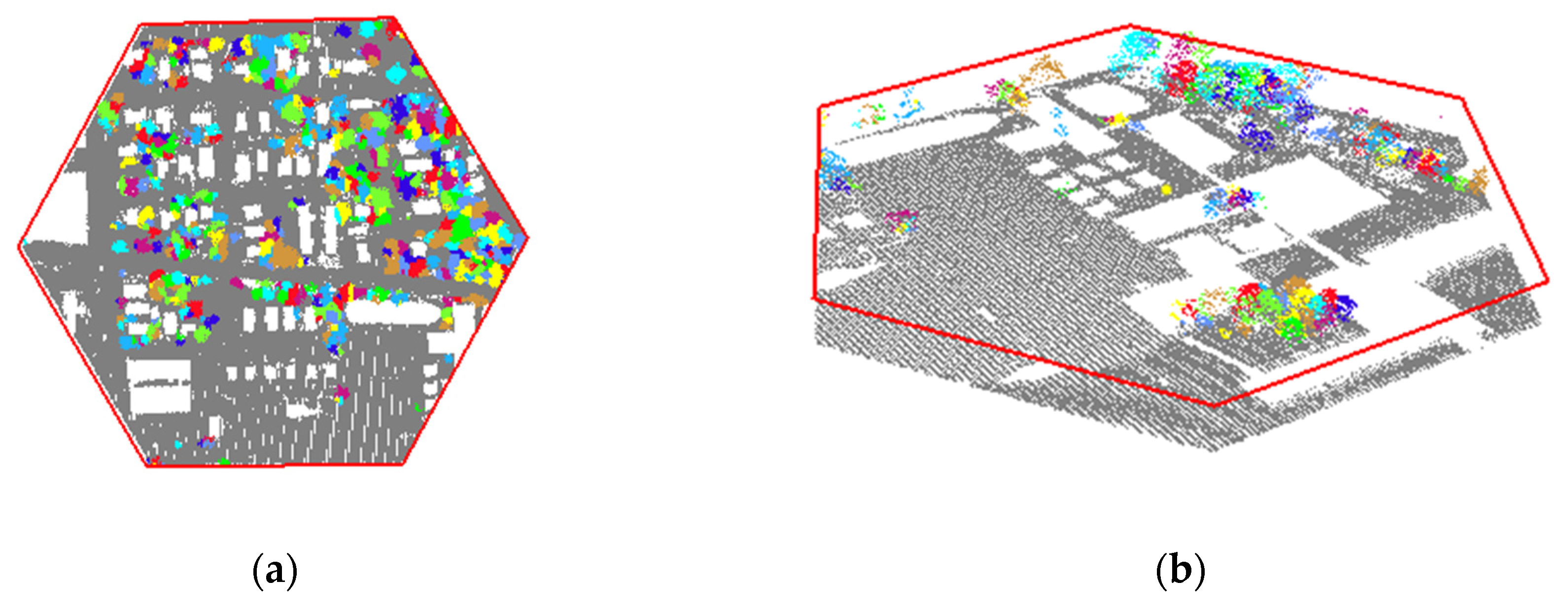
The point-wise semantic label is determined based on the prediction score vector after minimizing the loss function. Finally, the semantic segmentation maps the initial point cloud features to new high-level feature spaces. Namely, points of the same semantic category are clustered together, while the different classes are separated in the semantic feature space.

2.3. Graph-Structured Optimization for Classification Refinement

The proposed method exists a few local errors in the result of point-wise semantic learning network. For instance, a tree without canopy is misclassified as others or a pole mixed with tree is misclassified as a tree. Considering the object tree in the classification result as input in last step, instance segmentation of trees, these inaccurate labels may have undesirable consequences. Therefore, we can optimize the initial results and further obtain locally smoothed results with a probabilistic model. It is obvious that the wrong labels can be revised by their local context, as advocated in [52]. We model spatial correlations by applying a graph structure to ensure the consistency of point-wise label prediction, in other words, the labeling refinement can be converted into a graph-structured problem.
The first step is construction of the graph to structure the objective functional, the graphical model is constructed by the undirected adjacency graph G = { V , E } , where V = { v i } represents the nodes and a set of edges E = { e i j } encode spatial relationship of adjacent points with weights w. In graph G, for a central vertex v, we define its ten KNN neighbor according to the minimum number of edges from the other vertex v i to v. With respect to the edge weights w [ 0 ,   1 ] , the spatial distance, difference of normal vector angles and similarity are adopted for estimating weights. Furthermore, let p = { p 1 , , p N } denote a set of the points, let C = { c 1 , , c m } be a set of labels (in this paper, m is determined by the number of labels in the dataset), let Ψ = { Ψ | i = 1 , , N } represent a set of feature variables of points, and let L = { l = ( l 1 , , l N ) | l i C ,   i = 1 , , N } denote all possible label configurations [53]. To achieve global optimization using the constructed graph, we then formalize the optimal label configuration as an energy function minimization problem, and it is defined by following equation:
E ( L ) =   E d a t a ( L ) + λ E s m o o t h ( L )
where unary potential term E d a t a ( L ) quantitatively measures the disagreement between the possible label configuration L and the observed data, while smooth potential term E s m o o t h keeps smoothness and consistency between predictions, and λ is a weight coefficient used to balance the influence between the unary potential and the local smoothness.
With this configuration, the regularization process of the initial semantic segmentation will be performed to ensure labels locally continuous and globally optimal. In the proposed framework, the two terms have different definitions in the abovementioned energy functions. Consequently, the form of unary potential E d a t a ( L ) is typically:
E d a t a ( L ) = i V ϕ i ( l i )
where ϕ i ( l i ) measures how well label l i fits the feature variables Ψ i of given observed data and enforces the influence of the labels. As for the urban region, the same objects have similar features, while different objects have distinct features. The term ϕ i ( l i ) = log P ( l i ) is derived from the predicted probability P ( l i ) output from the point-wise classification. The higher the category posterior probability, the smaller the unary potential.
The second term in Equation (7) suppresses the “salt and pepper” effect and demonstrates the penalty to assign labels to a couple of 3D points, and is thus judged by E s m o o t h ( L ) = { i ,   j } E ψ i , j ( l i , l j ) = { i ,   j } E μ ( l i , l j ) p = 1 P ω p k ( f i , f j ) [54]. More specifically, μ ( l i , l j ) = 1 if l i l j or 0 otherwise, k represents the Gaussian kernel relying on extracted features f which is determined by the XYZ and intensity values of the points i and j, and ω p indicates constant coefficients. Two Gaussian kernels [55,56] are chosen as follows:
ω b e ( c o o r d i n a t e i c o o r d i n a t e j 2 2 θ α 2 intensity i intensity j 2 2 θ β 2 ) + ω s e ( c o o r d i n a t e i c o o r d i n a t e j 2 2 θ γ 2 )
where, ω b is the weight of the bilateral kernel, ω s is the weight of the spatial kernel, θ α , θ β and θ γ are three predefined hyperparameters.
While the regularization coefficient λ is estimated as follows:
λ = e d i j 2 δ 2
where d i j is the distance between points i and j, and δ is the expectation of all neighboring distances.
Accordingly, the optimal label prediction L * is the solution of minimization energy function with the following structure:
L * a r g min l C i V ϕ i ( l i ) + λ { i ,   j } E ψ i , j ( l i , l j )
Although accurate minimization is intractable, the minimization problem is easily and appropriately solved by a graph-cut algorithm using the α -expansion [57,58]. With a few graph-cut iterations, we can effectively and quickly find an approximate solution for optimizing multi-label energies. The labeling cost is not considered since graph-based optimization can effectively leverage the prediction and confidence, as well as semantic label assignment between two similar points in each region. The optimized results could be automatically adaptive to the underlying urban scenes without the predefined features for some uncertain objects.

2.4. Segmentation of Individual Roadside Trees with Deep Metric Learning

After the class 
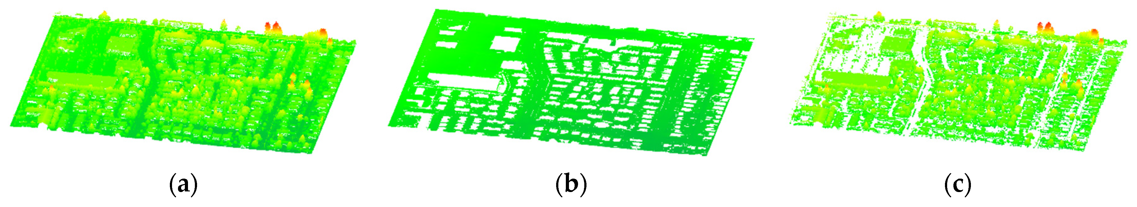
tree is determined, the label-based segmentation method is used to extract the tree points. As tree crowns are often clumped and connected together, it is vital to determine the points of individual trees by correctly isolating tree crown points of each trunk. Instance recognition of trees in environmentally complex urban areas is a challenge due to the poor-quality data. To overcome this problem, the quality of the segmented tree data is first enhanced through recovering the missing regions and removing the noise, outliers. We extend the previously proposed method in [59,60], and seek self-similar points to denoise them simultaneously using graph Laplacian regularization. Inspired by the algorithm of [61], we exploit an edge preserving smoothing algorithm using local neighborhood information to recover the regions with missing data. Delineation of individual trees from points after quality correction is then performed.
To automatically extract each tree crown points, a novel end-to-end architecture is applied to individual tree segmentation, which combines structure-aware loss function and attention-based k nearest neighbor (KNN). The proposed framework is summarized in 
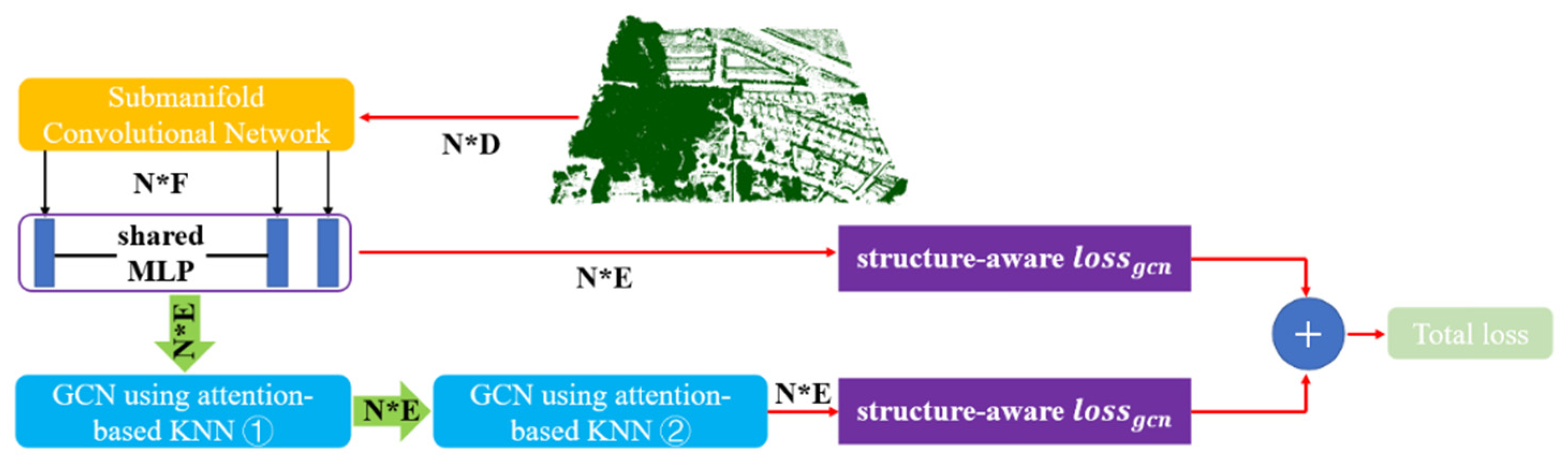
Figure 6, we elaborate on the three main components of our proposed network, including the submanifold convolutional network, the structure-aware loss function and the graph convolutional network (GCN), respectively. We firstly generate initial embeddings for each point by the submanifold sparse convolutional network. Inspired by the work of [62], we obtain discriminative embeddings for each tree from the LiDAR points based on the structure-aware loss function, which considers both the geometric and the embedding information. In order to achieve refined embeddings, we develop an attention-based graph convolutional neural network that aims to automatically choose and aggregate information from neighbors. Finally, to get segmentation of individual roadside trees, we employ a simple improved normalized cut segmentation algorithm to cluster refined embeddings.
Specifically, we directly use the architecture of the submanifold convolutional network (SCN) as our first component by borrowing from [63]. In our experiment, we use two backbone networks, including an UNet-like architecture (with smaller capacity and faster speed) and a ResNet-like architecture (with larger capacity and slower speed). In this section, we mainly describe the last two components of our proposed method for instance segmentation of trees. In the metric learning, the points within the same tree have similar embeddings while points from different trees are apart in the embedding space. Considering points within each tree do not only have embedding features but also have geometric relations, we hope that the final results will more discriminative by combining structure information with embedding features. Some commonly used metrics (e.g., cosine distance) for measuring the similarity between embeddings may cause the learning process and the post-process more difficult as kinds of reason. To make embedding discriminative enough, the Euclidean distance chosen to measure the similarity between embeddings after many test experiments. After measuring the similarity between embeddings, we obtain discriminative embeddings for each tree by a structure-aware loss function. Our loss function is consisted of the following two items:
s t r u c t u r e = 1 N i = 1 N i i n t r a + 1 N ( N 1 ) i = 1 N j = 1 , j i N i j i n t e r
where N is the total number of the tree in the entire scene. The first item i i n t r a aims to minimize the distance between embeddings within the same tree. As shown in Equation (13), the overall feature of a tree can be described by a mean embedding.
i i n t r a = j = 1 n i 1 1 + e s d i , j [ e d i , j α ] + 2
where α denotes a threshold for penalizing large embedding distance, n i is the point number of the ith tree. s d i , j is the coordinate of the jth point within the ith tree, which measures the spatial distance between the jth point and the geometric center μ s d , i of the ith tree; e d i , j is the embedding of the jth point within the ith tree, which measures the embedding distance between the jth point and the mean embedding μ e d , i . Further explanation, s d i , j and e d i , j are then represented as Equations (14) and (15), respectively.
s d i , j = s d j μ s d , i = s d j 1 n i j = 1 n i s d i , j
e d i , j = e d j μ e d , i = s d j 1 n i j = 1 n i e d i , j
On the other hand, the second item i j i n t e r is commonly used to make points from different trees discriminative. Specifically,
i j i n t e r = [ β μ s d , i μ s d , j ] + 2
where β denotes a threshold for the distance between mean embeddings. After repeated experiments, α and β is set 0.7 and 1.5 respectively.
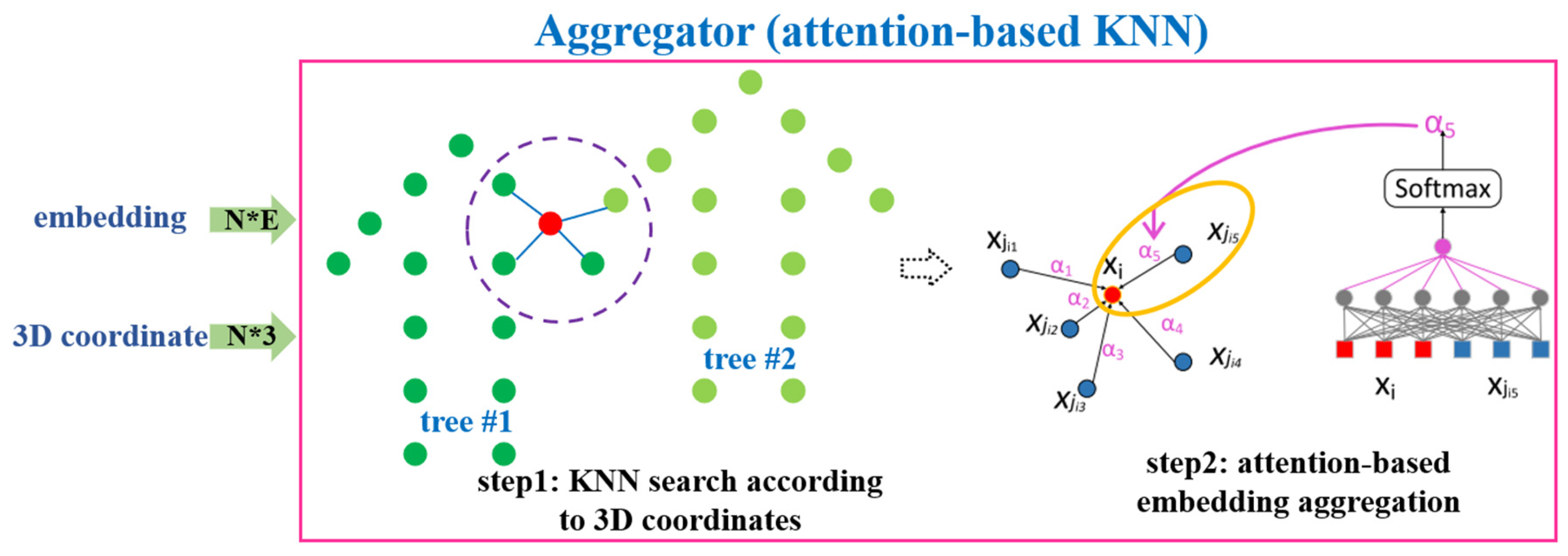
To achieve the goal that is to generate similar embeddings within the same tree and discriminative embeddings between different trees, KNN algorithm is applied to improve the local consistency of embeddings and aggregate information from surrounding points for a certain point. However, it is unfortunate that some wrong information brought by KNN will be harmful for embeddings. It is more obvious that a point near the edge of a certain tree may aggregates information from another trees. Instead of the standard KNN aggregation ( x i a g g r e g a t e ), an attention-based KNN is developed for embedding aggregation ( x i a g g r e g a t e ), which can assign different weights for different neighbors. The transform process can be formalized as follows:
x i a g g r e g a t e = 1 k m = 1 k x j i m x i a g g r e g a t e = m = 1 k α m x j i m
where the input embeddings of point clouds are denoted by X = { x 1 , , x n } R F , { x j i 1 , , x j i k } are the k nearest neighbors of x i according to their spatial positions, and α m is the attention weight for each neighbor and the normalization of the softmax function.
Figure 7 is the illustration of attention-based KNN which is the aggregator of our proposed graph convolutional neural network containing two steps. In step 1, for each input point, k nearest neighbors are searched according to the spatial coordinate. Different weights are assigned to different neighbors in step 2. The output of the aggregator is the weighted average of the embeddings of k neighbors. In general, aggregator in the form of attention-based KNN is a natural and meaningful operation for 3D points and allows the network to learn different importance for different neighbors.
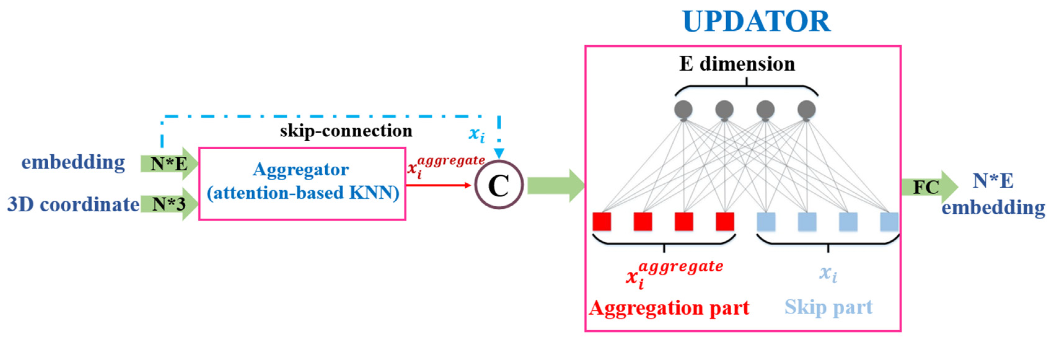
In the previous research, the GCN is normally composed of two parts: the aggregator and the updator (illustrated in Figure 8). As explained above, the aggregator is to gather information from neighbors using the proposed attention-based KNN. To update the aggregated information by mapping embeddings into a new feature space, a simple fully connected layer without bias is used as the updator. The operation is formalized as follows:
x i u p d a t e = [ x i , x i a g g r e g a t e ] W ,
where W R 2 F × F is a trainable parameter of the updator.
A portion of GCNs describe the relation using the laplacian matrix and the eigen-decomposition, which require huge computing cost (complexity O ( n 2 ) ). In contrast to previous GCNs, the main spotlight of our spatial GCN is that the attention-based KNN is used as the aggregator. In other word, the KNN (complexity O (n × k)) is used to describe the relation. It is quite vital for GCN to be applied to the original data. Last but not least, the proposed network will be easily trained end-to-end and uses the ADAM optimizer with constant learning rate 0.001. During implementation, we firstly pretrain the backbone network to obtain a pretrained segmentation model, then train the whole tree segmentation network based on the pretrained model, which can save time when conducting multiple experiments.
The spatially independent trees are quickly and effectively separated, but the overlapping or adjacent trees are difficult to isolate. Several previous researches reduced omission errors by a certain graph-cut algorithm, which enhanced accuracy but increased computational complexity. To further segment those objects containing more than one object, a supervoxel-based normalized cut segmentation method is developed. The mixed objects are firstly partitioned into homogeneous supervoxels with approximately equal resolution using the existing over-segmentation algorithm proposed in [64], which can preserve the boundary of object much better than others. Then, consider a complete weighted graph G(V, E) constructed from the given supervoxels according to their spatial neighbors, where the vertices V are represented by the center of supervoxels, and edges E are connected between each pair of adjacent supervoxels. The meaningful weight assigned to the edge is adopted for measuring the similarity between a pair of supervoxels connected by the edge and is calculated by the geometric information associated with the supervoxels as follows:
ω i j = { e x p ( ( D i j X Y ) 2 σ X Y 2 ) e x p ( ( D i j Z ) 2 σ Z 2 ) e x p ( ( G i j m a x ) 2 σ G ) , D i j X Y r X Y 0 , D i j X Y > r X Y
where D i j X Y and D i j Z are the horizontal and vertical distance between supervoxels i and j, respectively. σ X Y , σ Z and σ G indicate the standard deviations of D i j X Y , D i j Z and G i j m a x , respectively. r X Y is a distance threshold for determining the maximal valid distance between two supervoxels in the horizontal plane. G i j m a x is expressed as
G i j m a x = m a x ( D X Y ( i ,   t r e e T o p ) , D X Y ( j ,   t r e e T o p ) )
where D X Y ( i ,   t r e e T o p ) and D X Y ( j ,   t r e e T o p ) denote the horizontal distance between supervoxels i, j and the top of nearest tree.
Specifically, the similarity between two supervoxels is measured by considering their distance in the horizontal plane and their relative horizontal and vertical distributions. By such a definition, we partition the complete weighted graph G into two disjoint groups A and B by normalized cut segmentation method, which maximizes the similarity within each group ( A B = ) and the dissimilarity between two groups ( A B = V ). According to [65], the corresponding cost function is defined as
N c u t ( A , B ) = c u t ( A , B ) a s s o c ( A , V ) + c u t ( A , B ) a s s o c ( B , V )
where c u t ( A , B ) = i A , i B ω i j denotes the sum of the weights on the edges connecting groups A and B; a s s o c ( A , V ) = i A , i V ω i j and a s s o c ( B , V ) = i B , i V ω i j denote the sum of the weights on the edges falling in group A and B, respectively.
The process of dividing the weighted graph G into two separate groups A and B is regarded as the minimization of N c u t ( A , B ) . Since minimization problem is NP-hard, the proposed method relies on the approximation strategy, which achieves fairly good results in terms of solution quality and speed. Then the minimization of N c u t ( A , B ) is obtained by solving the corresponding generalized eigenvalue problem
( D W ) y = λ D y
where W(i, j) = ω i j , and D is a diagonal matrix, whose ith row records the sum of the weights on the edges associated with supervoxel i
D ( i , j ) = { m V ω i m ,   i f   i = j 0 , o t h e r w i s e
We introduce a parameter z denoted as D 1 2 y , thus, the Equation (22) is represented as D 1 2 ( D W ) D 1 2 z = λ z . From the basic principle of the Rayleigh quotient, it can be known that solving the minimum value problem of N c u t ( A , B ) is converted into solving the second minimum eigenvector of the feature system, and the best division result of normalized segmentation is obtained.
z = a r g min z T z 0 = 0 z T D 1 2 ( D W ) D 1 2 z z T z y = a r g min y T D y 0 = 0 y T ( D W ) y y T D y
where { λ = 0 ,   z 0 = D 1 2 I } is the small solution of the abovementioned feature system, y 0 = I is the smallest feature vector.
Based on the normalized cut principle, the overlapping objects are divided into two segments by employing a threshold to the eigenvector associated with the second smallest eigenvalue. Since elements of the second smallest eigenvector generally appear as continuous real values, a separation point needs to be introduced to bisect, usually 0 or the median of the eigenvector elements is used as the separation point. In order to minimize N c u t ( A , B ) , heuristic method [66] is used to find the optimal separation point. The elevation information plays a significant role in aerial LiDAR data processing, we finally adopt an elevation-attention module [67] which directly applies the per-point elevation information to improve segmentation results.

3. Results

A brief description about the experimental data is first given in this section. Then, we qualitatively and quantitatively analyze the performance of the results derived from the proposed method, respectively.

3.1. Data Description

We assess the performance of our approach using the following two public datasets: 2019 IEEE Geoscience and Remote Sensing Society (GRSS) Data Fusion Contest 3D point cloud classification challenge (DFC 3D) [68] and Dayton Annotated LiDAR Earth Scan (DALES) [69] dataset. The DFC 3D is an aerial LiDAR dataset, which is collected by the IEEE GRSS and covers approximately 100 km2 over parts of Southern United States, provided in ASCII text files. Considering the difference in category definition, we investigate six predefined semantic classes, namely, ground, tree, building, water, elevated road/bridge and unlabeled points. The XYZ and intensity are used as the inputs in our experiments. Scenes from three different types areas are provided on the IEEE GRSS 3D labeling website: two scenes with 10 files are employed as the training set and the other one scene with 6 files are used as the test set.
The DALES dataset is also composed of ALS data acquired with a Riegl LiDAR system flown with a mean flying height of about 1000 m above some Canadian cities. As a new large-scale ALS dataset, it spans 10 km2 of area and eight object categories with over 0.5 billion labeled points. The dataset is randomly split into two regions, namely training set and testing set with roughly a 70/30 percentage split, respectively.

3.2. Classification Performances

We quantitatively assess the classification performance of the proposed approach in terms of the following evaluation metrics [70]: precision, recall, F1 score, overall accuracy (OA), and average F1 score (AvgF1). Among them, the first three metrics are specifically applied to assess the performance on each single class, whereas overall accuracy and average F1 score are used to evaluate the performance on the whole test set. To test the performance of the improved network based on pointwise KNN search, the comparisons between the results with the original PointNet is conducted. Furthermore, to validate the feasibility of the graph-structured optimization designed for labeling refinement, the comparisons between the results with and without smoothing is conducted. Here, Table 1 and Table 2 list the final classification results on the DFC 3D dataset and the DALES dataset, respectively. More specifically, we finally achieved the precision of 87.0%, recall of 91.2%, and F1 score of 89.1% for labeling the tree class on the DFC 3D dataset, and an IoU of 94.1% for tree category on the DALES dataset.

3.2.1. Comparison between PointNet and Our Method

For the point-wise semantic segmentation, the feature learning of ALS data is a fundamental problem that directly affects the results of urban scene understanding. To validate the classification performance of the proposed network, we compared the results obtained by extracting more powerful local information using an optimized PointNet by KNN to those by extracting global features directly from the original PointNet. The classification results of original and optimized PointNet on the DFC 3D dataset are presented as a comparison in Table 3. The proposed network can largely improve the performance of classification with an increase of 10.7% in OA and a 19.9% increment in AvgF1. Additionally, the precision, recall, and F1 of tree show remarkable increase by 0.7%, 11.6%, 6.1%, respectively, indicating that the proposed strategy can produce higher accuracy, especially for the tree object extraction. The possible explanation is that the induction of multi-scale local information can provide better representation, especially in improving object integrity. Figure 9 presents the visualization of the classification results on DFC 3D dataset, it can be seen that the use of optimized PointNet procedure provides good initial result, which shows the efficacy of the proposed network in providing informative features.

3.2.2. Effectiveness of Labeling Smoothing Using Graph-Structured Optimization

There exists a small number of wrongly labeled points in the outputs, which can be corrected in the labeling smoothing by contextual information. In order to evaluate the usefulness of graph based-optimization, a regularization framework was tested for obtaining spatially smooth semantic labelling of UAV-LS data from a pointwise classification. Here, Table 4 lists the initial and optimized results of semantic segmentation, it can be seen that the overall performance does not show considerable improvements, the implementation of label smoothing improves the OA by 0.2%, but the influence of classification optimization is clear in some specific classes such as trees. Figure 10 shows the detailed visual illustration, which indicates an improvement in both smoothness and classification performance. As aforementioned, although wrongly classified points of most urban scenes are correctly labeled through a powerful deep learning method, the change in the statistic of the classification accuracies not seems apparent. This can be attributed to the reason that our strategy has already provided global and local properties with high quality, especially the implementation of the pointwise KNN search strategy.

3.2.3. Comparison with Other Published Methods

Additionally, we implemented several 3D semantic segmentation approaches to make a fair comparison using the above-mentioned two public dataset; such a comparison can reveal that the proposed method can outperform other classic methods.
After illustrating the effectiveness, we compare the proposed method with other published high-accuracy methods that have available codes using the DFC 3D dataset, including DANCE-Net [71] and GA-Conv [67]. The DANCE-Net method [71] classified the ALS data by introducing a density-aware convolution module which uses the point-wise density to reweight the learnable weights of convolution kernels and further developing a multi-scale CNN model to perform per-point semantic labeling. In GA-Conv method [67], whose strategy is similar to that of the DANCE-Net [71], approximating convolution on unevenly distributed 3D point sets with a geometry-attentional network consisting of geometry-aware convolution, dense hierarchical architecture and elevation-attention module to embed the three characteristics effectively, which can be trained in an end-to-end manner. Furthermore, compared to the aforementioned methods, the proposed method that also operates directly on point clouds, ranks second among three strategies, with OA value that are 5.1% higher than those of GA-Conv [67]. Table 5 displays a comparison of the classification accuracy with the aforementioned evaluation metrics among three different methods. Compared to DANCE-Net [71], we achieve a lower OA; however, we provide improved performance in classifying tree that produce a higher accuracy.
To further investigate the versatility of the proposed method on large-scale ALS datasets, we also obtained the pointwise classification results on the DALES dataset. We follow the evaluation metrics of similar large-scale LiDAR point cloud benchmarks and use the mean IoU and the OA as our main evaluation metrics. The per class IoU is first defined as Equation (25), the mean IoU is simply the mean across all eight categories, excluding the unknown category, of the form as Equation (26), and the OA can be calculated as Equation (27). For further evaluation, the proposed method was compared to previous published methods (we selected only algorithms that have published results and available codes, including PointNet++ [30], ShellNet [72], and Superpoint Graphs [42]). Quantitative comparison results on the DALES dataset are listed in Table 6, showing that the proposed network achieves better classification performance in terms of OA and mean IoU score than the other models. Specifically, the proposed model obtains state-of-the-art extraction performance for the trees. The notably strong performance of our architecture on trees with an IoU of 94.1%, over 2% higher than other networks is likely due to the difference between the proposed architecture and other methods, is that we did not rely on the selection of a fixed number of points within a search radius. This method of batch selection makes it possible to select a wide enough neighborhood to adequately get information while also having enough points to identify small objects.
I o U i = c i i c i i + j i c i j + k i c k i
I o U ¯ = i = 1 N I o U i N
O A = i = 1 N c i i j = 1 N k = 1 N c j k

3.3. Segmentation Performances of Individual Trees

3.3.1. Roadside Trees Segmentation

Figure 11 and Figure 12 illustrate the roadside trees segmentation results for the selected point clouds test data 1, test data 2 from DFC 3D dataset, respectively. Figure 11a and Figure 12a indicate the two selected scenes, colored by the elevation of each point. After ground points removed by the IPTD filtering algorithm, the road facilities were semantically recognized from the non-ground points. Figure 11b and Figure 12b show the object recognition results dotted in different colors, where gray, red, orange, green and blue points represent points from ground, buildings, water, trees and others respectively. Figure 11c and Figure 12c show roadside trees extraction outcomes, where tree is drawn in green and ground is dotted in gray. Figure 11d and Figure 12d show roadside trees instance segmentation outcomes, dotted in different color. Just like Figure 11 and Figure 12, Figure 13a–d and Figure 14a–d show the visualized results of each step of our method on the DALES dataset. More details of the individual roadside tree segmentation result are shown in Figure 15, Figure 15a is the segmentation outcomes for small trees and Figure 15b is segmentation outcomes for incomplete trees. It can be seen that the trees are well detected if they are not seriously overlaid, implying that the proposed method provides good performance in instance recognizing roadside trees, even small and incomplete objects.

3.3.2. Evaluation of the Proposed Method

We ran the tree segmentation algorithm in Python and compared the result with the reference trees. In this study, the performance of the proposed individual tree segmentation method on these two ALS datasets is evaluated by the following metrics [6]: segmentation accuracy (AC), omission error (OM) and commission error (COM). AC is the rate of trees correctly detected; OM is the rate of undetected trees, and COM is the rate of falsely detected trees.
AC = se/ref
OM = use/ref
COM = fse/ref
where de is the number of trees correctly segmented, ude is the number of unsegmented trees, fde is the number of trees falsely segmented and ref is the number of reference trees.
Table 7 shows the segmentation accuracy, omission error and commission error of individual tree segmentation from these two datasets. Our method achieves good results in segmenting roadside trees with an average AC, OM and COM of (86.8%, 13.2%, 9.5%) for the two datasets. Three metrics decline slightly with the sharp increasing scene complexity.

3.3.3. Comparative Studies

To evaluate the effectiveness of the instance segmentation of tree, we designed a group of experiments and compared it with other three methods, including Li’s method [73], ForestMetrics [74], and treeseg [75] in terms of segmentation accuracy, omission error, and commission error for recognizing roadside trees, as listed in Table 8. We apply the same data to evaluate the proposed method and other methods in this paper.
Li et al. [73] adopted a top-to-bottom region-growing method for tree segmentation in coniferous forests. However, the performance of the algorithm is not ideal when applied to urban roadside trees. ForestMetrics [74] mainly detects trunks and delineates individual trees from ALS to be well suited for trees with crowns of structurally complex shapes by a new bottom-up algorithm. Although ForestMetrics achieved a good tree segmentation performance with the AC, OM, and COM values of 85.9%, 14.1%, and 11.8%, respectively. Unfortunately, it fails to deal with extended and irregular tree shapes, especially if the canopy border is not correctly depicted. The data-driven approach, treeseg [75], utilizes generic point cloud processing techniques including Euclidean clustering, principal component analysis, region-based segmentation, shape fitting, and connectivity testing. The open-source approach to automate tree segmentation task, which uses few a priori assumptions of tree architecture, achieved worse segmentation accuracies with the AC, OM, and COM values of 80.9%, 19.1%, and 13.2%, respectively.
The proposed method employs an attention-based GCN which can automatically choose and aggregate information from neighbors, and a structure-aware loss function for tree segmentation to improve the geometric and the embedding information distinctiveness for individual tree. The proposed method also develops a novel and effective supervoxel-based normalized cut segmentation method, improving segmentation performance for incomplete and small trees. Thus, we have better accuracy of tree segmentation than those of Li’s method [73], ForestMetrics [74], and treeseg [75].

4. Conclusions

To address the complicated problem of classifying large-scale scenes and segmenting individual roadside trees objects, we proposed a complete workflow from airborne LiDAR data in environmentally complex urban areas, including (1) an improving progressive TIN densification filtering algorithm is applied to remove ground points, (2) a deep learning framework that integrates a point feature learning network, and a local feature learning network for the efficient semantic parsing of large-scale UAV-LS data, (3) a graph-structured optimization model to ensure the consistency of point-wise label prediction, (4) a simple yet novel method employing graph embedding learning with a structure-aware loss function and supervoxel-based normalized cut segmentation for isolating individual roadside trees. Our approach was evaluated by estimating accuracy on two publicly accessible ALS datasets, resulting in a satisfactory detection and segmentation of tree points from connected and clumped objects.
The experimental results demonstrate that our method provides a powerful solution to segment individual trees from urban UAV-LS data in terms of accuracy and correctness. It performed better than several classic 3D semantic segmentation methods and individual tree segmentation methods in terms of detection and segmentation accuracy. The proposed approach only utilizes 3D coordinates and intensity of point clouds and does not require any supplementary information, and is also robust to detect and segment roadside tree objects in overlapped region. The instance segmentation of tree from UAV-LS data also lay a good foundation for accurately calculating the structure metrics of trees and classification of species of urban trees, providing a good database for environmental impact assessment, biomass estimation, and tree risks management. In the future, we will test the proposed method on more large-scale road environment to build a complete roadside tree objects database for planning and management of urban forests.

Author Contributions

Conceptualization, Yongjun Wang, Tengping Jiang and Jing Liu; data curation, Yongjun Wang and Tengping Jiang; formal analysis, Tengping Jiang, Jing Liu and Xiaorui Li; funding acquisition, Yongjun Wang; investigation, Tengping Jiang and Chong Liang; methodology, Yongjun Wang and Tengping Jiang; project administration, Yongjun Wang; resources, Yongjun Wang and Chong Liang; software, Tengping Jiang; supervision, Yongjun Wang and Jing Liu; Validation, Xiaorui Li; visualization, Tengping Jiang and Xiaorui Li; writing—original draft, Yongjun Wang, Tengping Jiang and Jing Liu; writing—review and editing, Yongjun Wang, Tengping Jiang and Jing Liu. All authors have read and agreed to the published version of the manuscript.

Funding

This research described in this paper was jointly funded by the National Natural Science Foundation of China under Grant 41771439, the National Key Research and Development Program of China under Grant 2016YFB0502304, the Postgraduate Research and Practice Innovation Program of Jiangsu Province under Grant KYCX18_1206 and the Open Fund of Key Laboratory of Urban Land Resources Monitoring and Simulation, Ministry of Natural Resources under Grant KF-2018-03-070.

Acknowledgments

Special thanks to some open source projects, e.g., ForestMetrics and treeseg, they gave us great and valuable inspiration. Thanks to the visualization service provided by the LiDAR360 developed by Green Valley.

Conflicts of Interest

The authors declare no conflict of interest.

Appendix A

Algorithm A1: KNN-based local feature extraction
Input: point cloud P, D = { p 1 , p 2 , ,   p n   } , the dimension of each point is d;
Output: point cloud P, D = { p 1 , p 2 , ,   p n   } , the dimension of each point is d;
Parameter:K for KNN search
Step 1: The calculation of the feature distance between any pair of points.
Initialization: Define the similarity matrix S n × n between point pairs.
For i = 1, 2, …, n do
  The calculation of the Euclidean distance S i j = x i x j 2 F of the feature space between point x i and individual points x j (1 j n);
End For
Step 2: Select K neighboring points of each query point.
Initialization: Define the K-nearest neighbor matrix E N × K of each point and each local neighborhood feature matrix E N × d , where d is the feature dimension.
For i = 1, 2, …, n do
  Extract the distance vector S i = { S i 1 , S i 2 , ,   S i n   } between point x i and other points;
  Sort the vector S i from small to large, and select the top K elements, E i K = [ e 1 ,   e 2 , ,   e n ] ;
  Extract the d-dimensional local features F i = M A X { h ( x i ) , h ( x e 1 ) , h ( x e 2 ) , , h ( x e k ) } (where h is MLP) of point x i and K neighboring regions using MLP and max pooling layers;
End For
Step 3: Update the feature of each query point.
For i = 1, 2, …, n do
  For point x i , update the feature of the given point as x i = F i .
End For

References

  1. Roy, S.; Byrne, J.; Pickering, C. A systematic quantitative review of urban tree benefits, costs, and assessment methods across cities in different climatic zones. Urban For. Urban Green. 2012, 11, 351–363. [Google Scholar] [CrossRef] [Green Version]
  2. Islam, M.N.; Rahman, K.S.; Bahar, M.M.; Habib, M.A.; Ando, K.; Hattori, N. Pollution attenuation by roadside greenbelt in and around urban areas. Urban For. Urban Green. 2012, 11, 460–464. [Google Scholar] [CrossRef]
  3. Chen, Y.; Wang, S.; Li, J.; Ma, L.; Wu, R.; Luo, Z.; Wang, C. Rapid Urban Roadside Tree Inventory Using a Mobile Laser Scanning System. IEEE J. Sel. Top. Appl. Earth Observ. Remote Sens. 2019, 12, 3690–3700. [Google Scholar] [CrossRef]
  4. Ian, S.; Nikhil, N.; Carlo, R.; Raphäel, P. Green streets—Quantifying and mapping urban trees with street-level imagery and computer vision. Landsc. Urban Plan. 2017, 165, 93–101. [Google Scholar]
  5. Xu, Z.; Shen, X.; Cao, L.; Nicholas, C.; Tristan, G.; Zhong, T.; Zhao, W.; Sun, Q.; Ba, S.; Zhang, Z.; et al. Tree species classification using UAS-based digital aerial photogrammetry point clouds and multispectral imageries in subtropical natural forests. Int. J. Appl. Earth Obs. Geoinf. 2020, 92, 102173. [Google Scholar] [CrossRef]
  6. Yan, W.; Guan, H.; Cao, L.; Yu, Y.; Li, C.; Lu, J. A Self-Adaptive Mean Shift Tree-Segmentation Method Using UAV LiDAR Data. Remote Sens. 2020, 12, 515. [Google Scholar] [CrossRef] [Green Version]
  7. Yang, J.; Kang, Z.; Cheng, S.; Yang, Z.; Akwensi, P.H. An Individual Tree Segmentation Method Based on Watershed Algorithm and Three-Dimensional Spatial Distribution Analysis from Airborne LiDAR Point Clouds. IEEE J. Sel. Top. Appl. Earth Observ. Remote Sens. 2020, 13, 1055–1067. [Google Scholar] [CrossRef]
  8. Falkowski, M.J.; Smith, A.M.S.; Gessler, P.E.; Hudak, A.T.; Vierling, L.A.; Evans, J.S. The influence of conifer forest canopy cover on the accuracy of two individual tree measurement algorithms using lidar data. Can. J. Remote Sens. 2008, 34, S338–S350. [Google Scholar] [CrossRef]
  9. Lähivaara, T.; Seppänen, A.; Kaipio, J.P.; Vauhkonen, J.; Korhonen, L.; Tokola, T.; Maltamo, M. Bayesian Approach to Tree Detection Based on Airborne Laser Scanning Data. IEEE Trans. Geosci. Remote Sens. 2014, 52, 2690–2699. [Google Scholar] [CrossRef]
  10. Chen, Q.; Baldocchi, D.; Gong, P.; Kelly, M. Isolating Individual Trees in a Savanna Woodland Using Small Footprint Lidar Data. Photogramm. Eng. Remote Sens. 2006, 72, 923–932. [Google Scholar] [CrossRef] [Green Version]
  11. Vauhkonen, J.; Ene, L.; Gupta, S.; Heinzel, J.; Holmgren, J.; Pitkanen, J.; Solberg, S.; Wang, Y.; Weinacker, H.; Hauglin, K.M.; et al. Comparative testing of single-tree detection algorithms under different types of forest. Forestry 2011, 85, 27–40. [Google Scholar] [CrossRef] [Green Version]
  12. Polewski, P.; Yao, W.; Heurich, M.; Krzystek, P.; Stilla, U. Detection of fallen trees in ALS point clouds using a Normalized Cut approach trained by simulation. ISPRS J. Photogramm. Remote Sens. 2015, 105, 252–271. [Google Scholar] [CrossRef]
  13. Yang, B.; Dai, W.; Dong, Z.; Liu, Y. Automatic Forest Mapping at Individual Tree Levels from Terrestrial Laser Scanning Point Clouds with a Hierarchical Minimum Cut Method. Remote Sens. 2016, 8, 372. [Google Scholar] [CrossRef] [Green Version]
  14. Ferraz, A.; Bretar, F.; Jacquemoud, S.; Gonçalves, G.; Pereira, L.; Tomé, M.; Soares, P. 3D mapping of a multi-layered Mediterranean forest using ALS data. Remote Sens. Environ. 2012, 121, 210–223. [Google Scholar] [CrossRef]
  15. Zhen, Z.; Quackenbush, L.J.; Zhang, L. Trends in Automatic Individual Tree Crown Detection and Delineation—Evolution of LiDAR Data. Remote Sens. 2016, 8, 333. [Google Scholar] [CrossRef] [Green Version]
  16. Liu, L.; Lim, S.; Shen, X.; Yebra, M. A hybrid method for segmenting individual trees from airborne lidar data. Comput. Electron. Agric. 2019, 163, 104871. [Google Scholar] [CrossRef]
  17. Yan, W.; Guan, H.; Cao, L.; Yu, Y.; Gao, S.; Lu, J. An Automated Hierarchical Approach for Three-Dimensional Segmentation of Single Trees Using UAV LiDAR Data. Remote Sens. 2018, 10, 1999. [Google Scholar] [CrossRef] [Green Version]
  18. Li, S.; Zhou, C.; Wang, S.; Gao, S.; Liu, Z. Spatial Heterogeneity in the Determinants of Urban Form: An Analysis of Chinese Cities with a GWR Approach. Sustainability 2019, 11, 479. [Google Scholar] [CrossRef] [Green Version]
  19. Yang, B.; Dong, Z.; Zhao, G.; Dai, W. Hierarchical extraction of urban objects from mobile laser scanning data. ISPRS J. Photogramm. Remote Sens. 2015, 99, 45–57. [Google Scholar] [CrossRef]
  20. Xu, S.; Xu, S.S.; Ye, N.; Zhu, F. Automatic extraction of street trees’ nonphotosynthetic components from MLS data. Int. J. Appl. Earth Observ. Geoinf. 2018, 69, 64–77. [Google Scholar] [CrossRef]
  21. Babahajiani, P.; Fan, L.; Kämäräinen, J.K.; Gabbouj, M. Urban 3D segmentation and modelling from street view images and LiDAR point clouds. Mach. Vis. Appl. 2017, 28, 679–694. [Google Scholar] [CrossRef]
  22. Weinmann, M.; Weinmann, M.; Mallet, C.; Brédif, M. A Classification-Segmentation Framework for the Detection of Individual Trees in Dense MMS Point Cloud Data Acquired in Urban Areas. Remote Sens. 2017, 9, 277. [Google Scholar] [CrossRef] [Green Version]
  23. Guo, Y.; Wang, H.; Hu, Q.; Liu, H.; Liu, L.; Bennamoun, M. Deep Learning for 3D Point Clouds: A Survey. IEEE Trans. Pattern Anal. Mach. Intell. 2020. [Google Scholar] [CrossRef] [PubMed]
  24. Yang, Z.; Jiang, W.; Xu, B.; Zhu, Q.; Jiang, S.; Huang, W. A convolutional neural network-based 3D semantic labeling method for ALS point clouds. Remote Sens. 2017, 9, 936. [Google Scholar] [CrossRef] [Green Version]
  25. Yang, Z.; Tan, B.; Pei, H.; Jiang, W. Segmentation and multi-scale convolutional neural network-based classification of airborne laser scanner data. Sensors 2018, 10, 3347. [Google Scholar] [CrossRef] [Green Version]
  26. Zhao, R.; Pang, M.; Wang, J. Classifying airborne LiDAR point clouds via deep features learned by a multi-scale convolutional neural network. Int. J. Geog. Inf. Sci. 2018, 32, 960–979. [Google Scholar] [CrossRef]
  27. Te, G.; Hu, W.; Guo, Z.; Zheng, A. RGCNN: Regularized graph CNN for point cloud segmentation. In Proceedings of the ACM International Conference on Multimedia (MM), Seoul, Korea, 22–26 October 2018; pp. 746–754. [Google Scholar]
  28. Maturana, D.; Scherer, S. VoxNet: A 3D convolutional neural network for real-time object recognition. In Proceedings of the IEEE/RSJ International Conference on Intelligent Robots and Systems (IROS), Hamburg, Germany, 28 September–2 October 2015; pp. 922–928. [Google Scholar]
  29. Qi, C.R.; Su, H.; Mo, K.; Guibas, L.J. PointNet: Deep learning on point sets for 3D classification and segmentation. In Proceedings of the IEEE Conference on Computer Vision and Pattern Recognition (CVPR), Honolulu, HI, USA, 25–30 July 2017; pp. 652–660. [Google Scholar]
  30. Qi, C.R.; Yi, L.; Su, H.; Guibas, L.J. PointNet++: Deep hierarchical feature learning on point sets in a metric space. In Proceedings of the Neural Information Processing Systems (NIPS), Long Beach, CA, USA, 3–9 December 2017. [Google Scholar]
  31. Zhao, H.; Jiang, L.; Fu, C.W.; Jia, J. PointWeb: Enhancing local neighborhood features for point cloud processing. In Proceedings of the IEEE Conference on Computer Vision and Pattern Recognition (CVPR), Long Beach, CA, USA, 16–20 June 2019; pp. 5565–5573. [Google Scholar]
  32. Vaswani, A.; Shazeer, N.; Parmar, N.; Uszkoreit, J.; Jones, L.; Gomez, A.N.; Kaiser, Ł.; Polosukhin, I. Attention is all you need. In Proceedings of the Neural Information Processing Systems (NIPS), Long Beach, CA, USA, 3–9 December 2017. [Google Scholar]
  33. Zhao, C.; Zhou, W.; Lu, L.; Zhao, Q. Pooling scores of neighboring points for improved 3D point cloud segmentation. In Proceedings of the IEEE International Conference on Image Processing (ICIP), Taipei, Taiwan, China, 22–25 September 2019; pp. 1475–1479. [Google Scholar]
  34. Wang, S.; Suo, S.; Ma, W.C.; Pokrovsky, A.; Urtasun, R. Deep parametric continuous convolutional neural networks. In Proceedings of the IEEE Conference on Computer Vision and Pattern Recognition (CVPR), Salt Lake City, UT, USA, 18–22 June 2018; pp. 2589–2597. [Google Scholar]
  35. Thomas, H.; Qi, C.R.; Deschaud, J.E.; Marcotegui, B.; Goulette, F.; Guibas, L.J. KPConv: Flexible and deformable convolution for point clouds. In Proceedings of the IEEE International Conference on Computer Vision (ICCV), Seoul, Korea, 27 October–3 November 2019; pp. 6411–6420. [Google Scholar]
  36. Hua, B.S.; Tran, M.K.; Yeung, S.K. Pointwise convolutional neural networks. In Proceedings of the IEEE Conference on Computer Vision and Pattern Recognition (CVPR), Salt Lake City, UT, USA, 18–22 June 2018; pp. 984–993. [Google Scholar]
  37. Engelmann, F.; Kontogianni, T.; Leibe, B. Dilated point convolutions: On the receptive field of point convolutions. In Proceedings of the IEEE International Conference on Robotics and Automation (ICRA), Paris, France, 31 May–4 June 2020. [Google Scholar]
  38. Huang, Q.; Wang, W.; Neumann, U. Recurrent slice networks for 3D segmentation of point clouds. In Proceedings of the IEEE Conference on Computer Vision and Pattern Recognition (CVPR), Salt Lake City, UT, USA, 18–22 June 2018; pp. 2626–2635. [Google Scholar]
  39. Engelmann, F.; Kontogianni, T.; Hermans, A.; Leibe, B. Exploring spatial context for 3D semantic segmentation of point clouds. In Proceedings of the IEEE International Conference on Computer Vision (ICCV), Venice, Italy, 22–27 October 2017; pp. 716–724. [Google Scholar]
  40. Ye, X.; Li, J.; Huang, H.; Du, L.; Zhang, X. 3D recurrent neural networks with context fusion for point cloud semantic segmentation. In Proceedings of the European Conference on Computer Vision (ECCV), Munich, Germany, 8–14 September 2018; pp. 403–417. [Google Scholar]
  41. Liu, F.; Li, S.; Zhang, L.; Zhou, C.; Ye, R.; Wang, Y.; Lu, J. 3DCNN-DQN-RNN: A deep reinforcement learning framework for semantic parsing of large-scale 3D point clouds. In Proceedings of the IEEE International Conference on Computer Vision (ICCV), Venice, Italy, 22–27 October 2017; pp. 5678–5687. [Google Scholar]
  42. Landrieu, L.; Simonovsky, M. Large-scale point cloud semantic segmentation with superpoint graphs. In Proceedings of the IEEE Conference on Computer Vision and Pattern Recognition (CVPR), Salt Lake City, UT, USA, 18–22 June 2018; pp. 4558–4567. [Google Scholar]
  43. Liang, Z.; Yang, M.; Deng, L.; Wang, C.; Wang, B. Hierarchical Depthwise Graph Convolutional Neural Network for 3D Semantic Segmentation of Point Clouds. In Proceedings of the IEEE International Conference on Robotics and Automation (ICRA), Montreal, QC, Canada, 20–24 May 2019; pp. 8152–8158. [Google Scholar]
  44. Wang, L.; Huang, Y.; Hou, Y.; Zhang, S.; Shan, J. Graph Attention Convolution for Point Cloud Semantic Segmentation. In Proceedings of the IEEE Conference on Computer Vision and Pattern Recognition (CVPR), Long Beach, CA, USA, 16–20 June 2019; pp. 10288–10297. [Google Scholar]
  45. Li, Y.; Ma, L.; Zhong, Z.; Cao, D.; Li, J. TGNet: Geometric Graph CNN on 3D Point Cloud Segmentation. IEEE Trans. Geosci. Remote Sens. 2020, 58, 3588–3600. [Google Scholar] [CrossRef]
  46. Wang, X.; Liu, S.; Shen, X.; Shen, C.; Jia, J. Associatively segmenting instances and semantics in point clouds. In Proceedings of the IEEE Conference on Computer Vision and Pattern Recognition (CVPR), Long Beach, CA, USA, 16–20 June 2019; pp. 4096–4105. [Google Scholar]
  47. Zhang, K.; Chen, S.C.; Whitman, D.; Shyu, M.L.; Yan, J.; Zhang, C. A progressive morphological filter for removing nonground measurements from airborne LIDAR data. IEEE Trans. Geosci. Remote Sens. 2003, 41, 872–882. [Google Scholar] [CrossRef] [Green Version]
  48. Lin, X.; Zhang, J. Segmentation-based filtering of airborne LiDAR point clouds by progressive densification of terrain segments. Remote Sens. 2014, 6, 1294–1326. [Google Scholar] [CrossRef] [Green Version]
  49. Zhao, Q.; Guo, Q.; Su, Y.; Xue, B. Improved progressive TIN densification filtering algorithm for airborne LiDAR data in forested areas. ISPRS J. Photogramm. Remote Sens. 2016, 117, 79–91. [Google Scholar] [CrossRef] [Green Version]
  50. Zhang, W.; Qi, J.; Wan, P.; Wang, H.; Xie, D.; Wang, X.; Yan, G. An Easy-to-Use Airborne LiDAR Data Filtering Method Based on Cloth Simulation. Remote Sens. 2016, 8, 501. [Google Scholar] [CrossRef]
  51. Zhang, D.; He, F.; Tu, Z.; Zou, L.; Chen, Y. Pointwise Geometric and Semantic Learning Network on 3D Point Clouds. Integr. Comput. Aided Eng. 2020, 27, 57–75. [Google Scholar] [CrossRef]
  52. Wang, Y.; Jiang, T.; Yu, M.; Tao, S.; Sun, J.; Liu, S. Semantic-Based Building Extraction from LiDAR Point Clouds Using Contexts and Optimization in Complex Environment. Sensors 2020, 20, 3386. [Google Scholar] [CrossRef] [PubMed]
  53. Kang, Z.; Yang, J. A probabilistic graphical model for the classification of mobile LiDAR point clouds. ISPRS J. Photogramm. Remote Sens. 2018, 143, 108–123. [Google Scholar] [CrossRef]
  54. Qin, N.; Hu, X.; Wang, P.; Shan, J.; Li, Y. Semantic Labeling of ALS Point Cloud via Learning Voxel and Pixel Representations. IEEE Geosci. Remote Sens. Lett. 2020, 17, 859–863. [Google Scholar] [CrossRef]
  55. Wang, P.; Liu, Y.; Guo, Y.; Sun, C.; Tong, X. O-CNN: Octree-based convolutional neural networks for 3D shape analysis. ACM Trans. Graph. 2017, 36, 72. [Google Scholar] [CrossRef]
  56. Krähenbühl, P.; Koltun, V. Parameter learning and convergent inference for dense random fields. In Proceedings of the International Conference on Machine Learning (ICML), Atlanta, GA, USA, 16–21 June 2013; pp. 513–521. [Google Scholar]
  57. Kolmogorov, V.; Zabih, R. What energy functions can be minimized via graph cuts? IEEE Trans. Pattern Anal. Mach. Intell. 2004, 26, 147–159. [Google Scholar] [CrossRef] [Green Version]
  58. Xu, Y.; Ye, Z.; Yao, W.; Huang, R.; Tong, X.; Hoegner, L.; Stilla, U. Classification of LiDAR Point Clouds Using Supervoxel-Based Detrended Feature and Perception-Weighted Graphical Model. IEEE J. Sel. Top. Appl. Earth Observ. Remote Sens. 2020, 13, 72–88. [Google Scholar] [CrossRef]
  59. Zeng, J.; Cheung, G.; Ng, M.; Pang, J.; Yang, C. 3D Point Cloud Denoising using Graph Laplacian Regularization of a Low Dimensional Manifold Model. IEEE Trans. Image Process. 2020, 29, 3474–3489. [Google Scholar] [CrossRef] [Green Version]
  60. Osher, S.; Shi, Z.; Zhu, W. Low dimensional manifold model for image processing. SIAM J. Imaging Sci. 2017, 10, 1669–1690. [Google Scholar] [CrossRef]
  61. Huang, H.; Wu, S.; Gong, M.; Or, D.; Ascher, U. Edge-aware point set resampling. ACM Trans. Graph. 2013, 32, 9–21. [Google Scholar] [CrossRef]
  62. Liang, Z.; Yang, M.; Li, H.; Wang, C. 3D Instance Embedding Learning with a Structure-Aware Loss Function for Point Cloud Segmentation. IEEE Robot. Autom. Lett. 2020, 5, 4915–4922. [Google Scholar] [CrossRef]
  63. Graham, B.; Engelcke, M.; Maaten, L. 3d semantic segmentation with submanifold sparse convolutional networks. In Proceedings of the IEEE Conference on Computer Vision and Pattern Recognition (CVPR), Salt Lake City, UT, USA, 18–22 June 2018; pp. 9224–9232. [Google Scholar]
  64. Lin, Y.; Wang, C.; Zhai, D.; Li, W.; Li, J. Toward better boundary preserved supervoxel segmentation for 3D point clouds. ISPRS J. Photogramm. Remote Sens. 2018, 143, 39–47. [Google Scholar] [CrossRef]
  65. Yu, Y.; Li, J.; Guan, H.; Wang, C. Automated Extraction of Urban Road Facilities using Mobile Laser Scanning Data. IEEE Trans. Intell. Transp. Syst. 2015, 16, 2167–2181. [Google Scholar] [CrossRef]
  66. Reitberger, J.; Schnorr, C.; Krzystek, P.; Stilla, U. 3D segmentation of single trees exploiting full waveform LIDAR data. ISPRS J. Photogramm. Remote Sens. 2009, 64, 561–574. [Google Scholar] [CrossRef]
  67. Li, W.; Wang, F.; Xia, G. A geometry-attentional network for ALS point cloud classification. ISPRS J. Photogramm. Remote Sens. 2020, 164, 26–40. [Google Scholar] [CrossRef]
  68. LeSaux, B.; Yokoya, N.; Haensch, R.; Brown, M. 2019 IEEE GRSS data fusion contest: Large-scale semantic 3d reconstruction [technical committees]. IEEE Geosci. Remote Sens. Mag. 2019, 7, 33–36. [Google Scholar] [CrossRef]
  69. Varney, N.; Asari, V.K.; Graehling, Q. DALES: A Large-Scale Aerial LiDAR Data Set for Semantic Segmentation. Available online: https://arxiv.org/abs/2004.11985 (accessed on 1 June 2020).
  70. Huang, R.; Xu, Y.; Hong, D.; Yao, W.; Ghamisi, P.; Stilla, U. Deep point embedding for urban classification using ALS point clouds: A new perspective from local to global. ISPRS J. Photogramm. Remote Sens. 2020, 163, 62–81. [Google Scholar] [CrossRef]
  71. Li, X.; Wang, L.; Wang, M.; Wen, C.; Fang, Y. DANCE-NET: Density-aware convolution networks with context encoding for airborne LiDAR point cloud classification. ISPRS J. Photogramm. Remote Sens. 2020, 166, 128–139. [Google Scholar] [CrossRef]
  72. Zhang, Z.; Hua, B.; Yeung, S.K. ShellNet: Efficient point cloud convolutional neural networks using concentric shells statistics. In Proceedings of the IEEE International Conference on Computer Vision (ICCV), Seoul, Korea, 27 October–3 November 2019; pp. 1607–1616. [Google Scholar]
  73. Li, W.; Guo, Q.; Jakubowski, M.K.; Kelly, M. A New Method for Segmenting Individual Trees from the Lidar Point Cloud. Photogramm. Eng. Remote Sens. 2012, 78, 75–84. [Google Scholar] [CrossRef] [Green Version]
  74. Shendryk, I.; Broich, M.; Tulbure, M.G.; Alexandrov, S.V. Bottom-up delineation of individual trees from full-waveform airborne laser scans in a structurally complex eucalypt forest. Remote Sens. Environ. 2016, 173, 69–83. [Google Scholar] [CrossRef]
  75. Burt, A.; Disney, M.; Calders, K. Extracting individual trees from lidar point clouds using treeseg. Methods Ecol. Evolut. 2019, 10, 438–445. [Google Scholar] [CrossRef] [Green Version]
Figure 1. Pipeline of the proposed method.
Ijgi 09 00595 g001
Figure 2. The example of the filtering result. (a) Raw point cloud; (b) Ground points; (c) Non-ground points after ground removal.
Ijgi 09 00595 g002
Figure 3. The proposed point-wise semantic learning network architecture.
Ijgi 09 00595 g003
Figure 4. Illustration of the structure of the point feature extraction module.
Ijgi 09 00595 g004
Figure 5. Illustration of the structure of the local feature extraction module.
Ijgi 09 00595 g005
Figure 6. Illustration of the whole network architecture for individual tree segmentation. N is the number of points. F is the dimension of the backbone (submanifold convolutional network) output. E is the dimension of the instance embedding. The over-segmentation algorithm is used to cluster the instance embeddings during the inference.
Ijgi 09 00595 g006
Figure 7. Illustration of the aggregator using attention-based KNN.
Ijgi 09 00595 g007
Figure 8. Illustration of the updator part. The skip connection is used to concatenate the output of the aggregator and the input embedding together. Finally, a fully connected (FC) layer follows to update and get the refined output embedding.
Ijgi 09 00595 g008
Figure 9. Classification results of the DFC 3D dataset. (a) the classification result with PointNet; (b) the classification result with the proposed model; (c) the ground truth.
Ijgi 09 00595 g009
Figure 10. Detailed classification results of a certain selected area. (a) the initial classification result; (b) the smoothed classification result; (c) the ground truth.
Ijgi 09 00595 g010
Figure 11. Detailed results from selected area 1 of DFC 3D dataset. (a) the original point clouds; (b) the classification result; (c) the roadside trees extraction; (d) the roadside trees segmentation.
Ijgi 09 00595 g011
Figure 12. Detailed results from selected area 2 of DFC 3D dataset. (a) the original point clouds; (b) the classification result; (c) the roadside trees extraction; (d) the roadside trees segmentation.
Ijgi 09 00595 g012
Figure 13. Detailed results from selected area 1 of DALES dataset. (a) the original point clouds; (b) the classification result; (c) the roadside trees extraction; (d) the roadside trees segmentation.
Ijgi 09 00595 g013
Figure 14. Detailed results from selected area 2 of DALES dataset. (a) the original point clouds; (b) the classification result; (c) the roadside trees extraction; (d) the roadside trees segmentation.
Ijgi 09 00595 g014
Figure 15. Details of the roadside trees recognition outcomes: (a) small trees; (b) incomplete tree.
Ijgi 09 00595 g015
Table 1. Performance of classification results of our model with optimization using DFC 3D dataset. We report the precision, recall, and F1 score for each category in the first 3 columns as well as the OA and Avg F1 in the last two columns (All values are in %).
MetricsGroundBuildingsWaterOthersTreeOAAvg F1
precision94.592.890.765.787.091.182.9
recall96.195.632.483.191.2
F1 score95.394.249.286.989.1
Table 2. Overview of the proposed method on the DALES data set. We report the overall accuracy, mean IoU and per class IoU, for each category (All values are in %).
GroundBuildingsCarsTrucksPolesLinesFencesTreeOAMean
95.895.286.354.243.692.458.994.194.672.6
Table 3. Performance of our model and PointNet on the DFC 3D dataset. We report the precision (p), recall (r), and F1 score for tree category in the first 3 columns as well as the overall accuracy (OA) and average F1 score (Avg F1) in the last two columns (All values are in %).
MethodTree (p)Tree (r)Tree (F1)OAAvg F1
PointNet84.578.481.479.160.5
Ours (initial)85.290.087.589.880.4
Table 4. Comparison of the initial and smoothed classification results using DFC 3D dataset. We report the precision (p), recall (r), and F1 score for tree category in the first 3 columns as well as the OA and Avg F1 in the last two columns (All values are in %).
MethodTree (p)Tree (r)Tree (F1)OAAvg F1
Initial85.290.087.589.880.4
Smoothed87.091.289.191.182.9
Table 5. Quantitative comparison between our model and other methods on the DFC 3D dataset. We report the precision (p), recall (r), and F1 score for tree category in the first 3 columns as well as the overall accuracy (OA) and average F1 score (Avg F1) in the last two columns. The boldface text indicates the best performance (All values are in %).
MethodTree (p)Tree (r)Tree (F1)OAAvg F1
DANCE-Net87.489.987.093.878.0
GA-Conv78.693.085.886.074.7
Ours87.091.289.191.182.9
Table 6. Quantitative comparison between our model and other methods on the DALES 3D dataset. We report the overall accuracy, mean IoU and per IoU for tree category. Our model outperforms all other methods on the DALES dataset. We also note that all methods had a large variance between object categories. The boldface text indicates the best performance (All values are in %).
MethodTree (IoU)OAMean IoU
PointNet++81.985.763.1
ShellNet88.493.269.4
SuperPoint91.594.070.2
Ours94.194.672.6
Table 7. Individual tree segmentation results of the DFC 3D and DALES datasets using our method (All values are in %).
DatasetACOMCOM
DFC 3D85.114.910.2
DALES87.512.58.9
average86.813.29.5
Table 8. Comparison of tree segmentation performance among four different approaches (All values are in %).
MethodACOMCOM
Li [73]83.515.510.9
ForestMetrics85.914.111.8
treeseg80.919.113.2
Ours86.813.29.5

