Spatial and Temporal Patterns in Volunteer Data Contribution Activities: A Case Study of eBird


Department of Geography and the Environment, College of Natural Sciences and Mathematics, University of Denver, CO 80208, USA
ISPRS Int. J. Geo-Inf. 2020, 9(10), 597; https://0-doi-org.brum.beds.ac.uk/10.3390/ijgi9100597
Submission received: 2 September 2020
/
Revised: 6 October 2020
/
Accepted: 9 October 2020
/
Published: 11 October 2020
(This article belongs to the Special Issue Citizen Science and Geospatial Capacity Building)
Abstract
:Volunteered geographic information (VGI) has great potential to reveal spatial and temporal dynamics of geographic phenomena. However, a variety of potential biases in VGI are recognized, many of which root from volunteer data contribution activities. Examining patterns in volunteer data contribution activities helps understand the biases. Using eBird as a case study, this study investigates spatial and temporal patterns in data contribution activities of eBird contributors. eBird sampling efforts are biased in space and time. Most sampling efforts are concentrated in areas of denser populations and/or better accessibility, with the most intensively sampled areas being in proximity to big cities in developed regions of the world. Reported bird species are also spatially biased towards areas where more sampling efforts occur. Temporally, eBird sampling efforts and reported bird species are increasing over the years, with significant monthly fluctuations and notably more data reported on weekends. Such trends are driven by the expansion of eBird and characteristics of bird species and observers. The fitness of use of VGI should be assessed in the context of applications by examining spatial, temporal and other biases. Action may need to be taken to account for the biases so that robust inferences can be made from VGI observations.
1. Introduction
Empowered by the ubiquitous geospatial technologies such as global navigation satellite system trackers and location-aware smart phones, many ordinary citizens are now acting as human sensors and voluntarily contributing geo-referenced ground observations regarding a broad array of natural and social phenomena. Such geospatial data contributed by citizen volunteers are collectively referred to as volunteered geographic information (VGI) [1]. The most prominent VGI initiative is OpenStreetMap (OSM) [2], a platform on which volunteers compile map data (e.g., detailed streets, roads, points of interest etc.) for much of the world. eBird, a popular citizen science project [3,4], is yet another VGI platform where birdwatchers around the world contribute and share geo-referenced birding records on a daily basis. Data from such VGI platforms has been widely used, for example, to support land management, network modeling and routing [5], and biodiversity conservation and research [3,6].
VGI has a great potential for revealing spatial and temporal dynamics of the geographic phenomena under observation [7,8]. However, VGI data quality issues have long been under scrutiny and, particularly, a variety of potential biases in VGI are recognized [3,9,10,11,12,13,14,15]. In order to draw robust inferences from VGI, such biases need to be understood and properly accounted for in VGI data analyses [16,17,18]. Some of the biases (e.g., observer and taxonomic biases) can be attributed to volunteer contributors’ background (e.g., social, demographic and economic status, level of expertise); others are deeply rooted in their data contribution activities [3,19,20]. For example, individual volunteers have their own interests or motivations and often determine where and when to conduct observations at their own will, having no intent to coordinate sampling efforts with each other nor to follow any designed sampling scheme (e.g., stratified random sampling). As such, volunteer data contribution is often biased in space and time, which leads to biased spatial and temporal coverage in VGI observations. Examining spatial and temporal patterns in volunteer data contribution activities improves understanding of the spatial and temporal biases embedded in VGI. Such investigation in turn sheds light upon devising methods for bias mitigation to improve the reliability of inferences made from VGI [17,18]. It also helps identify any spatial and temporal observation gaps within VGI datasets toward which future sampling efforts can be directed.
A few studies have examined patterns in volunteer data contribution activities in various projects, and some consistent patterns exist. With respect to contributor variability, a relatively small share of volunteers often contribute most of the data whilst a large portion of contributors are ephemeral [19,21,22,23], which is a phenomenon of participation inequality consistently observed across online communities that is characterized by Zipf’s law and the 90-10-1 rule [24,25,26]. Regarding temporal variability, volunteer data contributions are very uneven across time [21]. For instance, most contributions to OSM were made during the afternoon and evening hours and more contributions were made on Sundays [22]. Twitter users tweet the most around 13:00–1400 and 20:00–21:00 throughout the week while Flickr users are more active during weekends and most photos are taken during the afternoon hours [23]. In terms of spatial variability, most geographic areas have few contributors and contributions and most contributions tend to cluster in major cities with high population density [23,27]. As for identifying the pattern-shaping factors, Bittner [28] identified social biases in data contributions to OSM and Wikimapia in Jerusalem, Israel. Boakes et al. [19] revealed species abundance, ease of identification and tree height were positively related to the number of records that contributed to three biodiversity citizen science projects in the Greater London area. Based on a study using data from four citizen science projects in Denmark, Geldmann et al. [29] suggested distance to roads, human population density and land cover can be used to account for spatial bias in volunteer sampling efforts. Li et al. [23] discovered that well-educated people in the occupations of management, business, science, and arts are more likely to be involved in the generation of georeferenced tweets on Twitter and photos on Flickr. Although these studies examined patterns in volunteer data contribution through an array of lenses, few have investigated the patterns along the spatial and temporal dimensions at the same time (except [23]). More research is also in need for modeling and understanding how various factors may shape volunteer data contribution patterns.
This study aims to thoroughly examine the spatial and temporal patterns in volunteer data contribution activities among eBird contributors. eBird was launched by the Cornell Lab of Ornithology and the National Audubon Society in 2002 and has become the world’s largest biodiversity-related citizen science project [3,30]. eBird data are freely accessible to anyone and have been used to support conservation decisions and help inform bird research worldwide [30]. Using the eBird mobile application or website, birders can upload information regarding when, where, and how they conduct birding and fill out a checklist of the birds seen and heard. As of 31 December 2019, over a half-million eBird contributors had collectively contributed over 50 million geo-referenced sampling events (i.e., checklists) containing more than 700 million bird observations on over 10,000 bird species across 253 countries and territories around the world [31].
The data contribution patterns in eBird have been examined through spatial or temporal profiling. For example, researchers profiled the number of submitted observations and checklists over the years 2003–2013 by month [3,6,32]. Yet, there lacks temporal profiling at finer granularity. In assessing global survey completeness of eBird data, La Sorte and Somveille [33] visualized the number of checklists, the number of species, and survey completeness (calculated by day, week, and month) based on data accumulated during 2002–2018 within equal-area hexagon cells that are 49,811 km2 in area at the finest spatial resolution. It is a rather coarse spatial resolution to reveal spatial patterns at finer spatial scales. Many of these results (except [33]) have been outdated given the fast-growing capacity of eBird. For instance, from 1 January 2015 through 31 December 2019, over 33 million new sampling events (~ 62% of the total) and 450 million new bird observations (~64% of the total) were submitted to eBird, and the cumulative number of contributors more than doubled [31]. The eBird website (ebird.org) provides interactive grid cell maps (~20 km resolution) showing the spatial distribution of the number of observed bird species and species relative frequency [34]. Such visualizations help understand trends in species distributions. However, they are not very useful for revealing the spatial and temporal patterns in birder’s data contribution activities (i.e., sampling efforts). In summary, an up-to-date, wholistic spatial and temporal profiling of the eBird data at finer spatial and temporal resolutions, and modeling effects of factors in shaping sampling efforts are much needed to better understand the status quo of data contribution patterns in VGI projects such as eBird and beyond.
This study reports a comprehensive profiling of eBird data to discover the spatial and temporal patterns in volunteer data contribution activities. Discovering the patterns helps understand spatial and temporal biases and thus informs better data use. It can also reveal spatial and temporal gaps in existing sampling efforts; birders may direct future birding efforts to under-observed regions and/or time periods to improve eBird data coverage. Besides, the effects of environmental and cultural factors in shaping the spatial pattern of volunteer sampling efforts is explored in this study through spatially explicit modeling. The modeling provisions quantitative information on spatial variation of sampling efforts, which may be incorporated into other modeling process (e.g., species distribution modeling) for explicitly accounting for spatial bias to improve modeling performance [29].
2. Materials and Methods
2.1. eBird Data
eBird data (version: July 2020) were requested and downloaded from the eBird website (ebird.org), and records with an observation date before or on 31 December 2019 were used for analysis in this study. The dataset contains sampling event data and bird observation data [31]. Essentially, sampling event data have records regarding where (latitude, longitude), when (observation date) and by whom (identified by observer id) each birding session (identified by sampling event identifier) was conducted. These records reflect birder’s sampling efforts. Bird observation data contain information on the observed bird species (identified by species scientific name) and their count estimates, among others, during each birding session. A bird observation can be related to a sampling event base on a common sampling event identifier present in both records.
eBird data were pre-processed, parsed and loaded into PostgreSQL/PostGIS, a free and open-source object-relational database with geospatial capabilities (postgis.net). As of 31 December 2019, a cumulative total of 548,365 eBird contributors (observers) had contributed 53,837,394 sampling events containing 716,876,356 bird observations on 10,379 bird species in 253 countries and territories around the world. The distribution of eBird data across the countries and territories is highly skewed (Table 1). The countries and territories with the 10 largest numbers of sampling events account for 89.9% of sampling events and 84.6% of sampling locations world-wide.
2.2. Visualizing Spatial and Temporal Patterns
The spatial and temporal patterns in data contribution activities of eBird contributors were examined by visualizing results of spatial and temporal queries and analyses on the eBird data. SQL (standard query language) queries were used to obtain summary statistics regarding sampling events, observers, and reported bird species. The first two statistics reflect sampling efforts of eBird contributors, whilst the third indicates observed diversity of bird species.
The above summary statistics were aggregated and mapped on a grid of 0.25° latitude × 0.25° longitude cells (~28 km × 28 km at the equator) across the globe to visualize spatial patterns. Temporal patterns were visualized by aggregating and plotting the summary statistics over time periods of various granularities (year, month, day of week). These visualizations together provide a wholistic view of the spatial and temporal patterns in the volunteer data contribution activities of eBird contributors.
2.3. Modeling Sampling Efforts
The above spatial and temporal visualizations, although useful to uncover spatial and temporal patterns in volunteer data contribution activities, provide little insights on the underlying drivers shaping the patterns. To this end, spatial modeling was conducted to identify and quantify the effects of environmental and cultural factors in shaping the current spatial patterns in sampling efforts of eBird contributors. The Maxent approach (Section 2.3.3) was adopted to model the spatial pattern in eBird sampling efforts based on sampling locations in the most recent full year of 2019 (Section 2.3.1) and covariate data characterizing environmental and cultural factors (Section 2.3.2).
2.3.1. Sampling Efforts
There were 2,131,692 geographically unique eBird sampling locations world-wide in 2019 (Figure 1). These sampling locations represent volunteer sampling efforts in a most recent full-year cycle. Note that locations on the sea represent observations made from ships.
2.3.2. Covariates
A set of five covariates representing environmental and cultural factors was used for modeling the spatial pattern in eBird sampling efforts. According to analyses of data from four citizen science projects in Denmark [29], land cover, population density and road density often are the major variables that determine spatial bias in citizen science. These covariates are indicators of vegetation/land use condition, human activity intensity and infrastructure. In addition, the country-level United Nations Human Development Index (HDI), a summary measure of average achievement in key dimensions of human development including life expectancy, years of education and gross national income per capita [35], was used in modeling because birding as a recreational activity is more often conducted by highly educated citizens with higher annual income [36]. Although the covariates are often correlated, each of them does contain a certain amount of independent information. Moreover, the Maxent modeling method used in this study (Section 2.3.3) does not require uncorrelated variables to achieve good model performance.
Besides, given that eBird is a global project with contributors from all over the world submitting data through either the eBird mobile app or website, contributor’s knowledge of the written language in which the app or website is available could also play a role in determining the large-scale spatial bias in eBird data. Specifically, as of August 2015, the eBird mobile app is only available in five languages including Spanish, French, Chinese (Traditional), German, and English [37], although more languages have been added since then. The language in which the app and website is available may impact where and who would use them for contributing data to eBird. Therefore, a country-level official language map was used as an additional cultural variable in modeling the spatial pattern in eBird sampling efforts. Note that although spoken languages often have ambiguous geographic boundaries, official languages have much more clearly delineated boundaries (e.g., political boundaries). Moreover, official languages, often including both the spoken and written components, are widely taught in a country’s school system.
A consensus world land cover dataset compiled by the EarthEnv project [38] was downloaded from here [39]. Population density map projected for 2020 produced by NASA’s Socioeconomic Data and Applications Center [40] was downloaded from here [41]. Road density data compiled by the Global Roads Inventory Project [42] were downloaded from here [43]. The road density was for all roads (highways, primary roads, secondary roads, tertiary roads, and local roads). The most recent release of 2018 HDI data [35] with HDI values for all United Nations member countries [35] were downloaded from here [44]. The country-level official language map compiled by CIA World Factbook, University of Groningen was downloaded through a web feature service here [45]. It contains the first, second and third (if any) official languages of each country. In this study, countries were categorized based on the ordered list of official languages. Land cover, population density, and road density data are in raster format at a spatial resolution of 30 arc seconds (about 1 km at the equator). The vector-format HDI map and language map were rasterized to the same spatial resolution as the other covariates (Figure 2).
Frequency distributions of the sampling locations on the covariates were plotted against their respective background frequency distributions (distributions of all covariate values across the world) (Figure 3). The background distribution of the official language covariate was computed as per-language percentages of the 2019 world population at the country level (population data were obtained here [46]). The background distribution of HDI was computed as frequency distribution of the country-level HDI values weighted by the population of each country in 2019. Relative frequencies of land cover type, population density and road density were computed as area percentage. The frequency distributions show that the sampling intensity of eBird contributors is higher in areas of cultivated and managed vegetation and in urban/built-up areas. Although only about 40% of the sampling locations are in areas with population density above 100 persons/km2, this is a high percentage considering the background distribution. About 75% of the sampling locations are in areas with road density greater than 250 m/km. Approximately 65% of the sampling locations are in countries where English is the official language (e.g., U.S. and U.K.) and another 10% in countries where Spanish is the official language. Finally, 80% of the sampling locations are in well-developed countries with HDI greater than 0.9. All indicate biases in sampling efforts along dimensions of the environmental and cultural factors.
2.3.3. Modeling Method
The Maxent (maximum entropy) approach [47] was adopted to model the spatial pattern in eBird sampling efforts. Maxent is a general-purpose machine-learning method for making predictions or inferences from incomplete information and it has been widely used in various application domains, for example, modeling species distribution based on species “presence-only” data (e.g., occurrence locations) [47] and modeling geographic distribution of tourists from the locations tourists visited [48]. Maxent is well suited for modeling eBird sampling efforts as birding locations are also “presence-only” data. A conceptual overview of the Maxent method is provided below (readers interested in the mathematical details are referred to [47]).
Maxent estimates a probability distribution over a geographic area consisting of discrete raster cells (probability surface) based on two inputs: localities indicating the occurrences of a target event and covariate data layers characterizing the environmental factors that affect the event’s occurrences. The probability of the event occurring at a cell is a function of the in-situ environmental conditions. The probability distribution is determined following the maximum entropy principle. That is, the distribution should be as close to a uniform distribution as possible while conforming to constraints embedded in the event occurrence localities. For example, expectation of the distribution on environmental variables should be close to the empirical averages observed at the occurrence localities. Maxent has been widely applied in various domains such as for modeling species geographic distribution [47] and for predicting geographic distribution of tourists [48].
In this study, eBird sampling locations (i.e., occurrence localities) and raster data layer of the four environmental and cultural covariates were input to Maxent to estimate the probability of a location being sampled by birders (sampling probability). The Maxent software version 3.4.0 [49] was used in this study. Most parameter settings of Maxent were kept to the defaults (e.g., auto feature, cloglog output format) as they have been fine-tuned on a large dataset and are supposed to work well in general [50]. Changes were made on four parameters. First, samples (eBird sampling locations) were not added to background as the author observed adding samples to background would greatly degrade model performance because the large number of sampling locations when added to background would severely bias background. Second, the number of background points was set to 500,000 (the default is 10,000) given the large study area (i.e., world continents and islands) from which random background points are selected. Third, the maximum number of iterations was changed from the default 500 iterations to 2,000 iterations to ensure the optimization procedure converges. Fourth, Maxent by default removes sample locations that are within the same raster cell of the covariates. This default setting was changed such that only duplicate locations with identical geographic coordinates were removed. Since the duplicates are removed by the model, information regarding repeated visits of the same location was not considered in the modeling process. The model thus effectively models the probability of the occurrence of at least one sampling event at a location, which is different to modeling the total spatial bias in eBird sampling efforts, as some sites/locations have many sampling events. After removing out-of-extent locations and duplicate locations, the number of eBird sampling locations was reduced to n = 1,920,182. Half of the locations (n = 960,091) were used for model training and the other half were used as test data for evaluating model performance.
Maxent model performance was evaluated by computing AUC (the area under the curve) of the predicted sampling probability map based on sampling locations in the test data and randomly selected background locations [50]. The AUC, a threshold-independent model performance measure, is the probability that the predicted sampling probability at a randomly chosen location will be higher than that at a randomly chosen background location [47]. The AUC ranges from 0 to 1, with AUC = 1 indicating perfect model performance, AUC = 0.5 indicating performance comparable to a random model, and AUC < 0.5 indicating worse-than-random model performance.
3. Results
3.1. Spatial and Temporal Patterns
3.1.1. Sampling Events
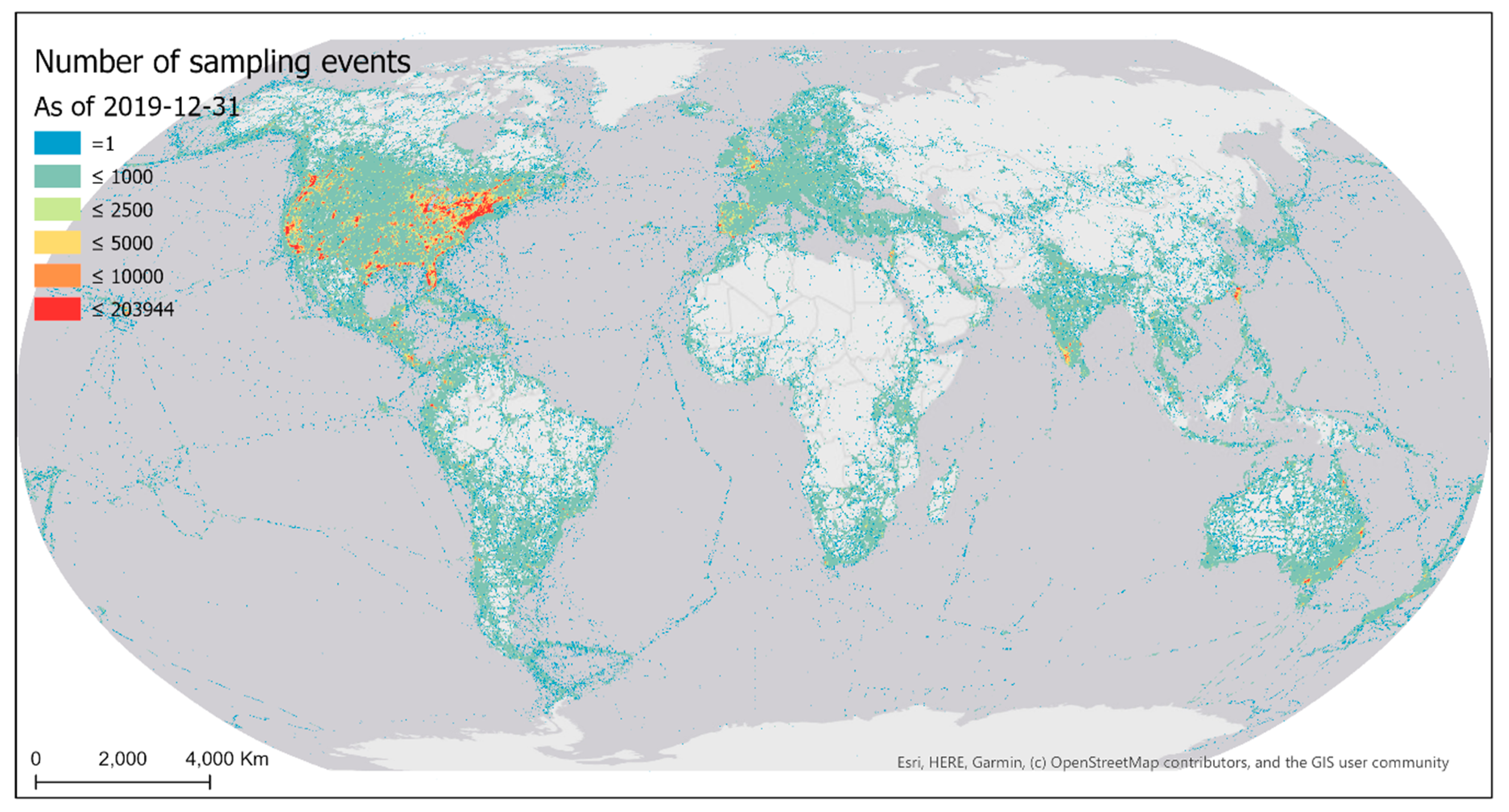
Sampling events conducted by eBird contributors were highly biased over the geographic space (Figure 4). Much of the world has not yet been sampled by eBirders. Among the grid cells that have been sampled, half have fewer than nine sampling events within a cell. Sampled areas are mostly developed regions of the world with better accessibility (e.g., higher road density). The most intensively sampled areas are in proximity to big cities of the world.
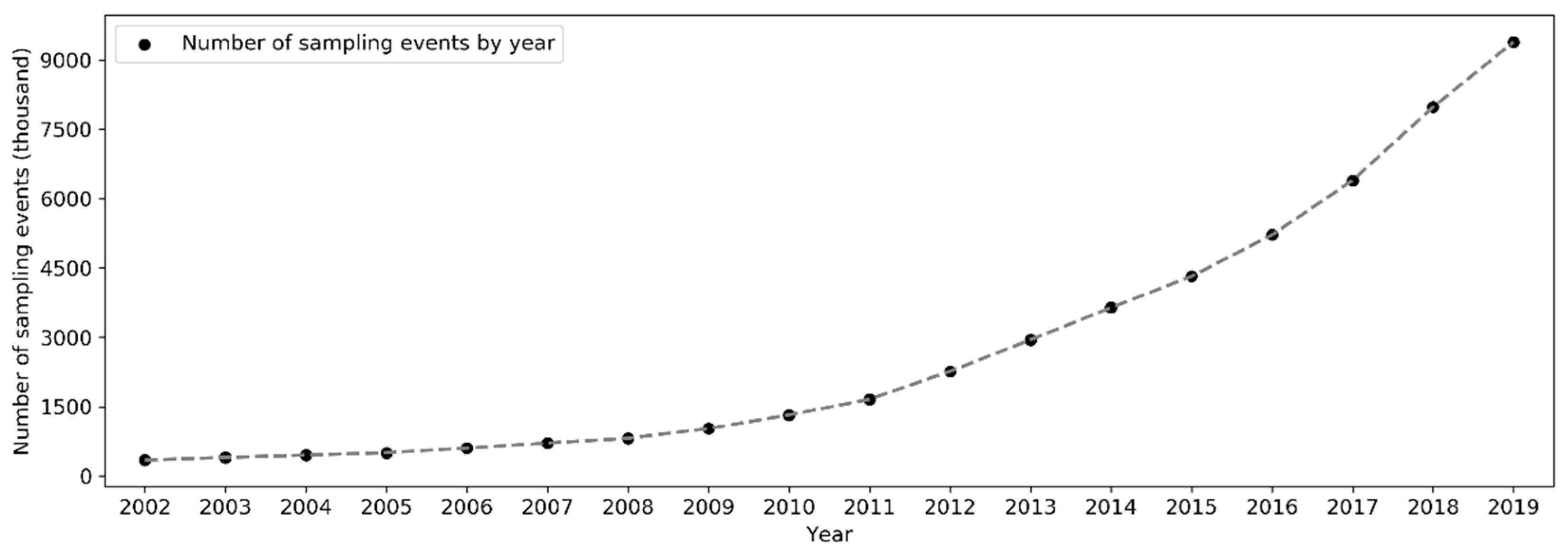
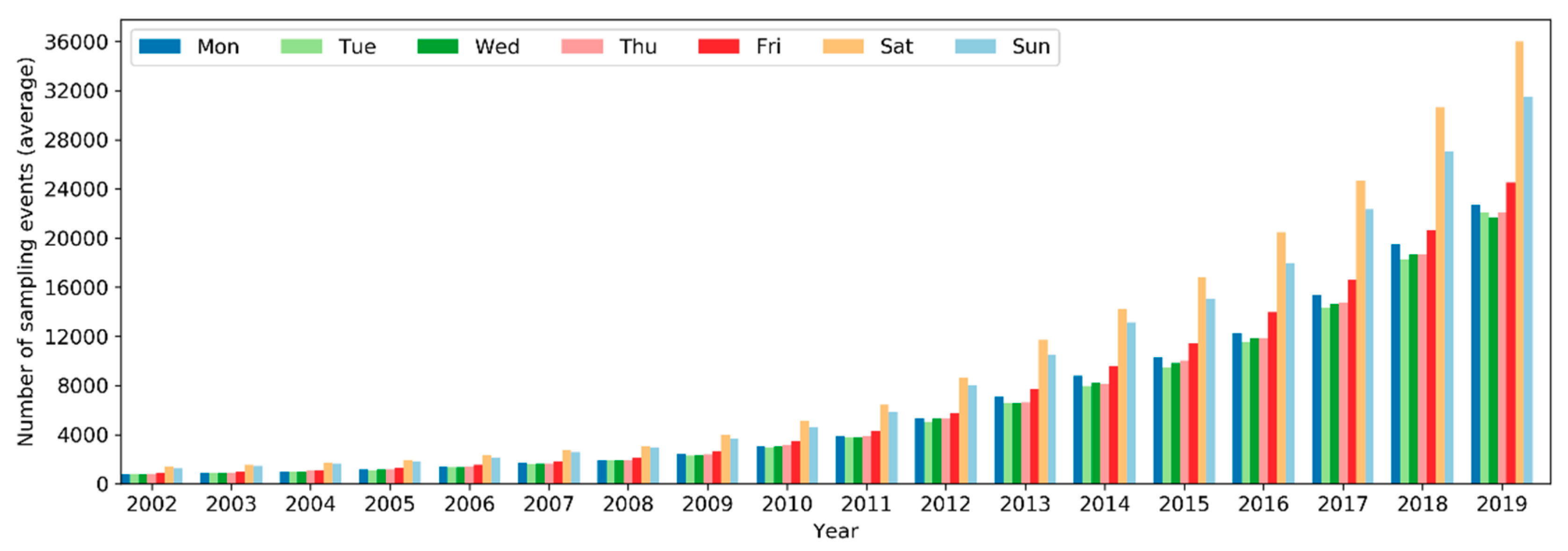
On a yearly basis, the total number of sampling events has been increasing exponentially (i.e., at a faster pace) since 2002 (Figure 5). Over the months of the years 2002–2019, the number of sampling events in the northern hemisphere increased starting from March or April and peaked in May (Figure 6). Sampling efforts then significantly decreased and reached the lowest in July or August. In the southern hemisphere, sampling events were the fewest in May or June and the most in October or November. The overall number of sampling events across the world followed a monthly trend similar to that in the northern hemisphere. Over the days of the week through the years (Figure 7), there were more sampling events on weekends than on weekdays.
The number of species reported across sampling events is skewed (Figure 8). On average, 13 species were reported in each sampling event. Yet, no more than nine species were reported in half of the sampling events. About 15.5% of the sampling events reported only a single species, 36.1% reported 2–10 species, 37.5% reported 10–30 species, and 10.6% reported 30 species or more.
There are sampling events associated with very large number of species. After checking records in the database, it was found there are n = 29 events with 300 or more observed species, and n = 480 events with 200 or more species (statistics obtained based on bird observations reviewed and approved by eBird). Most (n = 349) of the events have associated trip comments providing contextual information, although some are not in English. Overall, many of these events with large number of species are not ‘regular’ birding events. For example, some events are (1) compilations of birding records over prolonged birding periods (e.g., days or weeks), (2) records imported from publications, (3) birding events involving groups of birders who submitted records in a single record, (4) special birding events such as field guide, and (5) Big Day birding events where birders aimed to find as many birds as possible in a single day. Nonetheless, such birding events are not expected to have a significant impact on the reported statistics in this article (e.g., average number of species per event), given the very large sample size (n = 53,837,394 events in total).
3.1.2. Observers
The spatial distribution pattern of eBird contributors (observers) over the 0.25° latitude × 0.25° longitude grid cells (Figure 9) was similar to that of the sampling events. Among the grid cells that have been covered by observers, half of the cells have fewer than four contributing observers.
The number of active observers (observers who contributed at least one sampling event) has been increasing exponentially since 2002 (Figure 10). Notably, there was a significant boost in the number of observers in 2013. Over the months of the years (Figure 11), the highest peak in the number of active observers in the northern hemisphere occurred often in May, but since 2013 there was another peak in February. In the southern hemisphere, birders were most active in October or November, but since 2015 there was another peak in May (see Section 4.2.2 for possible explanations). The overall number of active observers across the world followed a monthly trend similar to that in the northern hemisphere. Over the days of the week (Figure 12), there were more active observers on weekends than on weekdays.
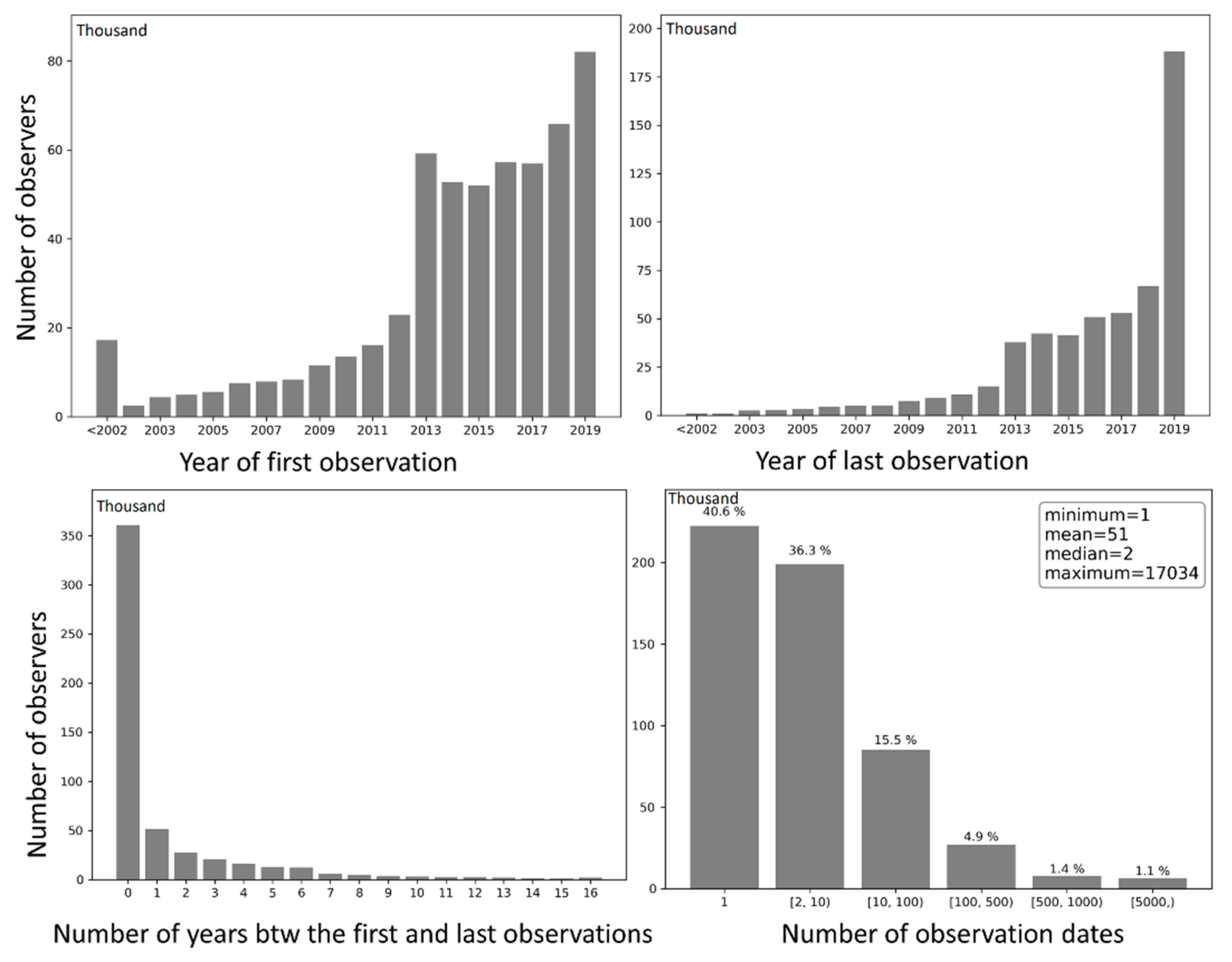
Observers were grouped by (1) the year in which they submitted the first observation to eBird, (2) the year in which they submitted the last observation, (3) the number of years between the first and last observations, and (4) the number of days with observations (Figure 13). Grouping results of (1) and (2) reflect the number of observers entering and exiting eBird each year (except for 2019), respectively. Over the years, the number of entering and exiting observers both increased approximately exponentially. There was a sharp rise in the number of observers entering eBird in 2013, followed by a slight decrease and plateau during 2014–2017, and a modest increase in 2018 and another significant leap in 2019. Grouping results of (3) and (4) reveal the temporal span of birding activities of the observers in units of year and day, respectively. About 67.9% of the observers contributed data only in a single year, 9.7% contributed in two consecutive years, 5.2% contributed in three consecutive years, and 17.2% contributed in four or more consecutive years. Speaking of the number of days with observation, 40.6% of the observers contributed observations on a single day, 36.3% contributed on 2–10 days, and 23.1% contributed on 10 or more days. Such patterns in contributors span over time are consistent with the life cycle of contributors in collaborative online communities [51].
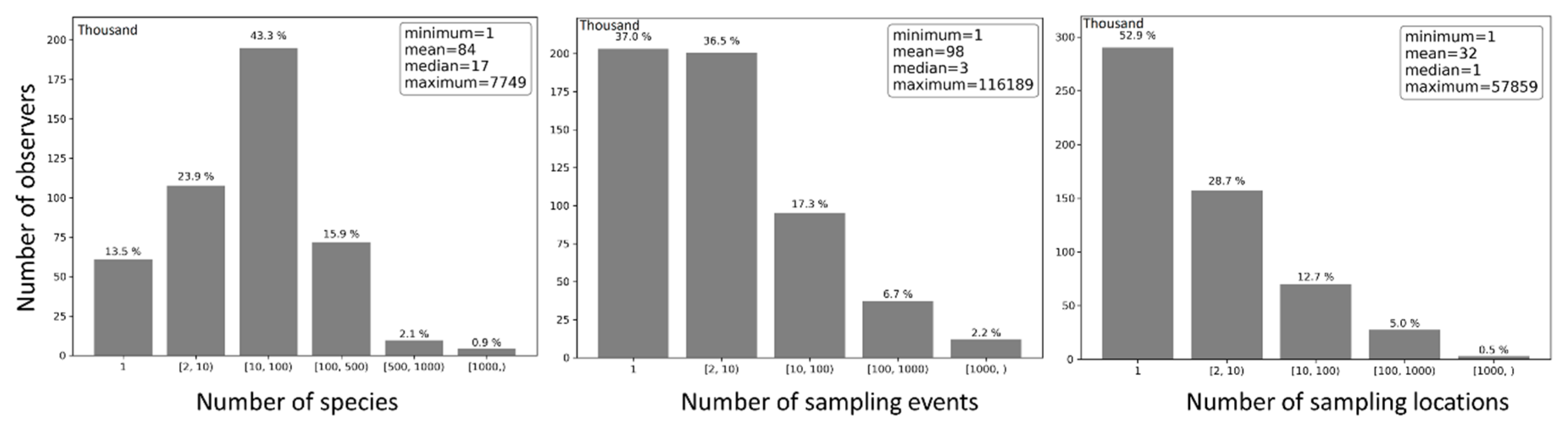
On average, each observer contributed 98 sampling events, sampled 32 locations, and reported 84 species (Figure 14). Nonetheless, half of the observers contributed no more than three sampling events, sampled only one location, and reported no more than 17 species. About 37% of the observers contributed just one sampling events, 53.8% contributed 2–100 sampling events, and 9.2% contributed 100 or more sampling events. Approximately 52.9% of the observers sampled only one location, 41.4% sampled 2–100 locations, and 5.7% sampled 100 or more locations. Roughly 13.5% of the observers reported only one species, 67.2% reported 2–100 species, and 19.3% reported 100 or more species.
3.1.3. Bird Species
The distribution of bird species reported by eBird contributors is also highly skewed and spatially biased (Figure 15). Many parts of the world still do not have any bird species reported because of the lack of sampling efforts in those areas (Section 3.1.1). Among the grid cells with bird observations, half of them have a number of reported bird species below 42.
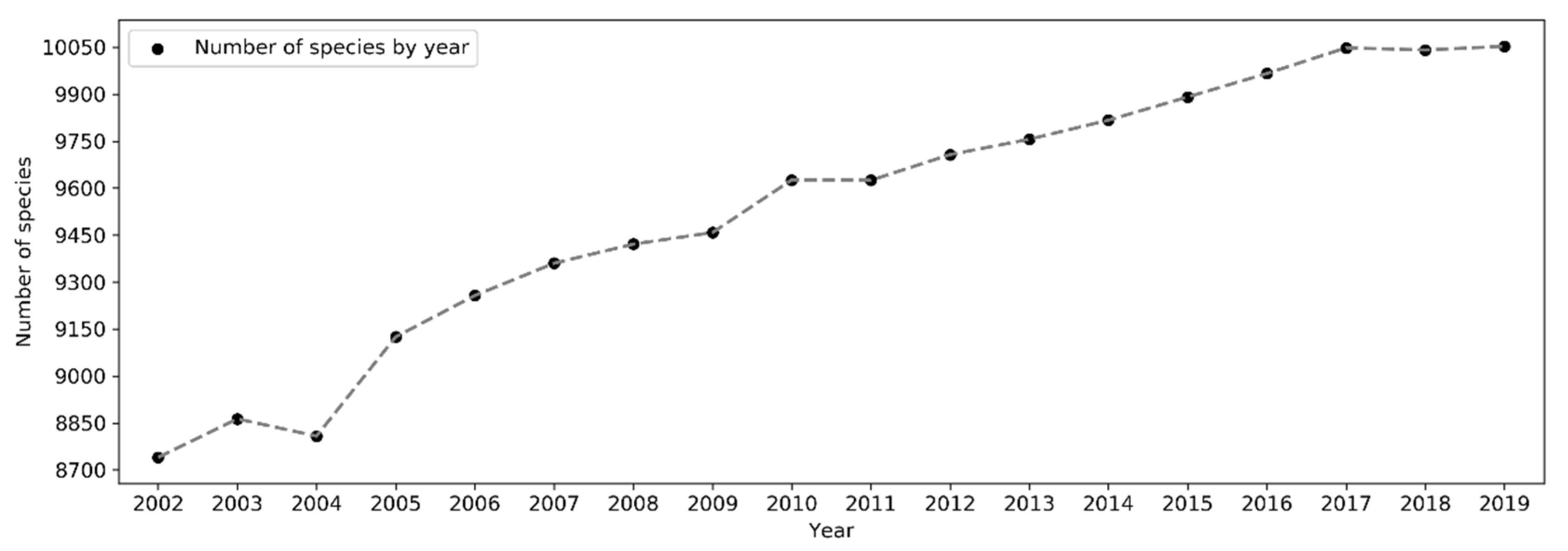
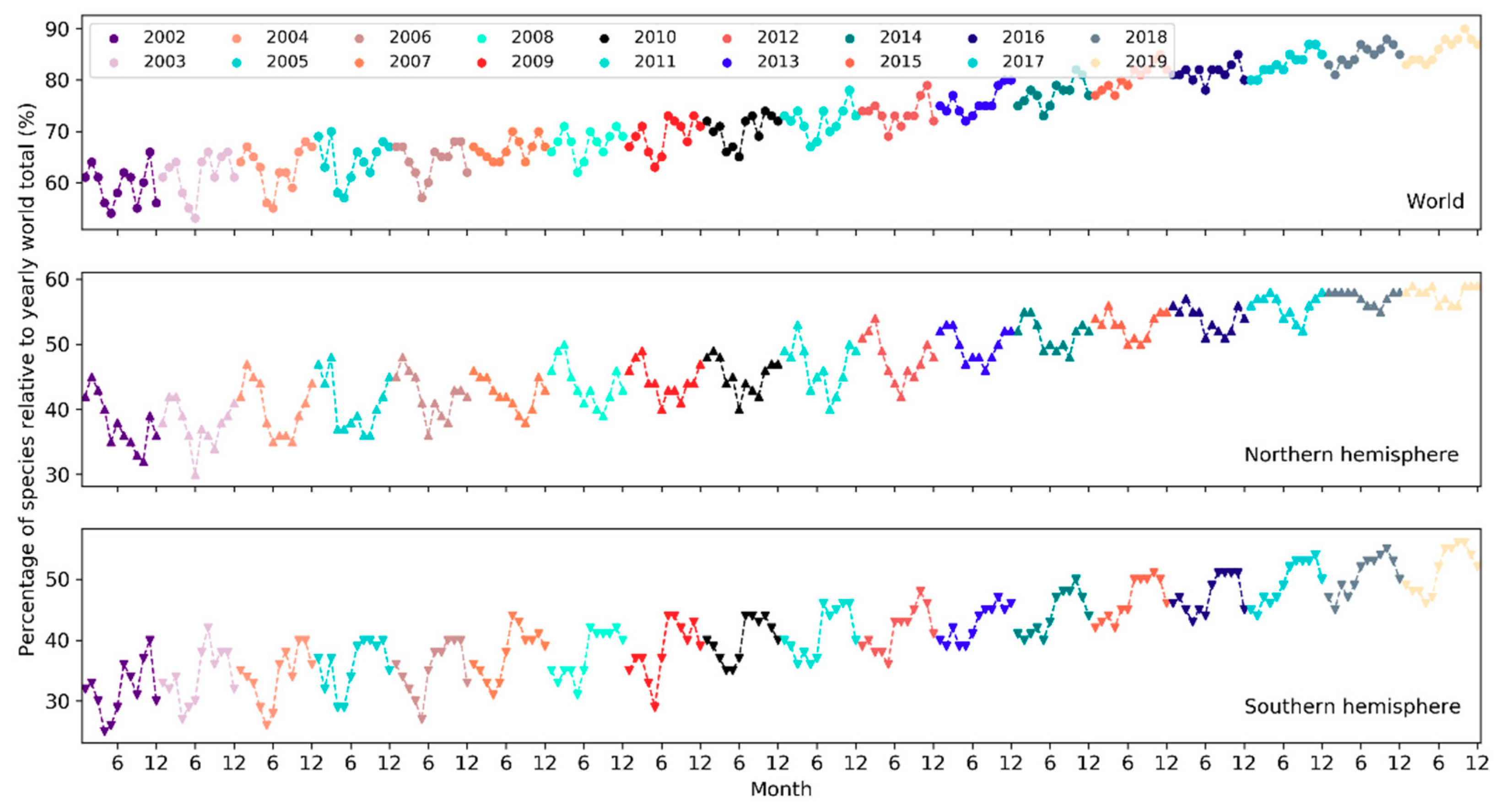
The total number of species reported to eBird in a single year has been increasing in a linear fashion since 2002 but plateaued starting 2017 (Figure 16). From 2002 to 2019, the number of reported bird species increased from 8,740 to 10,053 (~15% increase). There was a sharp rise in 2005 and yet another jump around 2010. A larger number of species were observed in November–March in the northern hemisphere whilst in July–November in the southern hemisphere (Figure 17). The overall number of reported species often peaked in October or November. Over the days of the week (Figure 18), a larger number of species were reported on weekends than on weekdays.
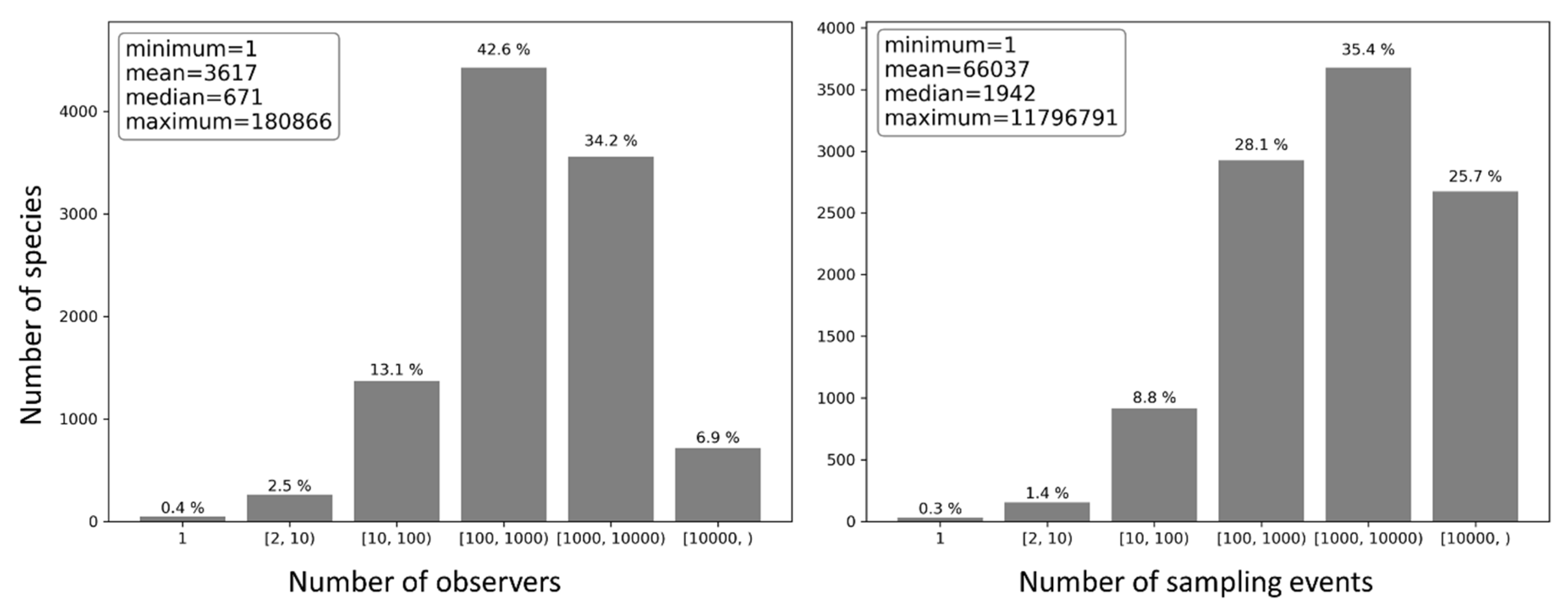
For each bird species present in the eBird database, the number of observers who reported the species and the number of sampling events in which the species was reported were counted (Figure 19). Half of the species were reported by no more than 671 observers and in no more than 1942 sampling events; on average, each bird species was reported by 3617 observers and in 66,037 sampling events, suggesting overall highly repetitive species observations. Only 0.4% of the species were reported by a single observer and 0.3% in a single sampling event, whilst about 83.7% of the species were reported by over 100 observers and 89.2% in over 100 sampling events.
3.2. Modeling Sampling Efforts
3.2.1. Analysis of Variable Importance
According to estimates of percent contributions of the environmental and cultural variables to the model provided in Maxent output (Table 2), road density and official language seem to be the two most important factors that contributed to the Maxent model. Land cover and HDI have much less contribution, and population density has very little contribution to the model. Permutation importance for each variable is the resulting drop in training AUC (normalized to percentages) when the values of that variable on training sampling and background locations are randomly permuted and the model is trained on the permuted data. Training AUC would drop the most when HDI values are permuted, followed by official language. Permutation on the other three variables would result in little drop in training AUC. It suggests that HDI and official language are important controlling factors determining birders’ sampling locations at large spatial scales (e.g., country-level).
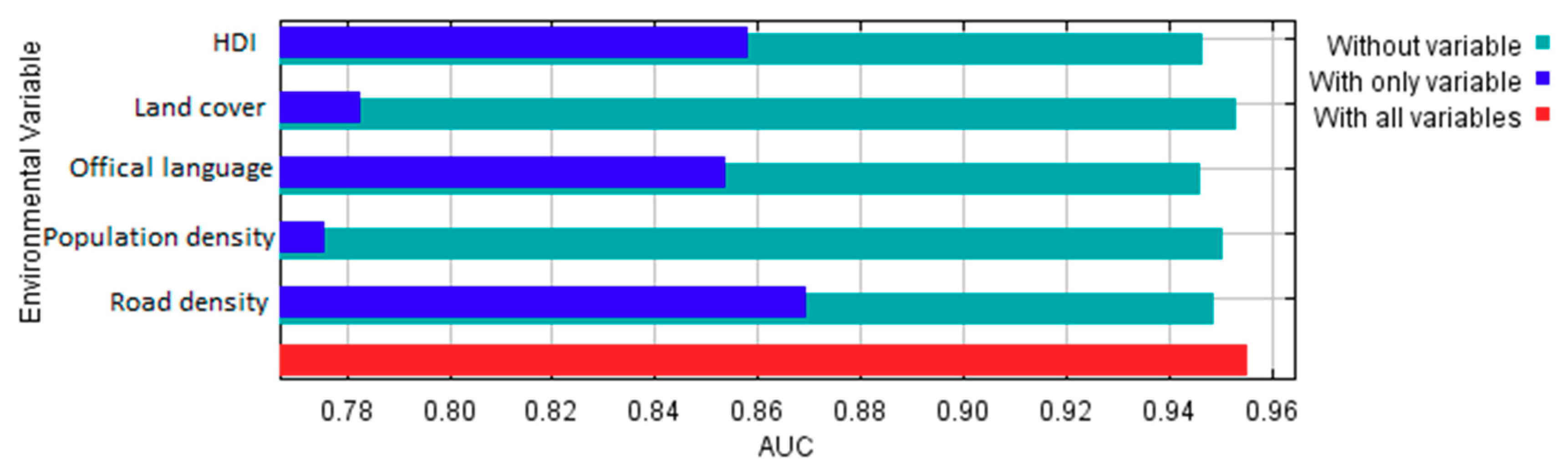
Moreover, based on the results of the jackknife test of variable importance (Figure 20), the variable with highest test AUC when used in isolation is road density, which therefore appears to have the most useful information by itself. By this standard, HDI and official language have slightly less useful information, and land cover and population have the least useful information. The variable that decreases test AUC the most when it is omitted is official language, which therefore appears to have the most information that is not present in the other variables. Nevertheless, the decreases in test AUC when omitting each variable is rather slight, meaning that using any four variables would result in model performance (as measured by the test AUC) very close to that of all five variables. Yet, variable contribution and variable importance should be interpreted with caution when the predictor variables are correlated. In this case, for example, there exist positive correlations between population density and road density at the raster cell level (Pearson’s r = 0.48, p < 0.001) and between HDI and mean road density at the country level (Pearson’s r = 0.27, p < 0.001).
3.2.2. Modeled Sampling Probability
The map of sampling probability of eBird contributors (i.e., probability of the occurrence of at least one sampling event) modeled and predicted using the Maxent method (with all five covariates) is shown in Figure 21. The AUC computed for the probability map based on the held-out test data is 0.955, indicating an excellent model performance. That is, the model generally predicts higher sampling probability values at sampling locations in the test data than at randomly selected background locations. Across the globe, English and Spanish-speaking countries have the highest modeled sampling probability. Other European countries and some countries in Asia also have higher modeled sampling probability. Interestingly, most countries with high modeled sampling probability are highly developed countries in the world. There exists much spatial variation in the modeled sampling probability within each country. For example, higher sampling probability was modeled in southern parts of Canada and the east half and west coast of the United States, particularly in the vicinity of big cities. In Australia, the highest sampling probability was found on the east and southeast coasts, especially in the vicinity of big cities. These areas and/or cities are where most population reside and most infrastructure (e.g., roads) have been built.
4. Discussion
4.1. Spatial Patterns in eBird Data
Existing eBird sampling efforts (sampling events and observers) were mostly concentrated in areas of denser populations and/or better accessibility (e.g., higher road density), with the most intensively sampled areas being in proximity to big cities in developed regions of the world (Figure 4 and Figure 9). Such spatial bias highlights significant disparities in the birding activities of eBird contributors across developed and under-developed regions. Due to the spatially biased sampling efforts, the number of reported bird species was also spatially biased towards areas where more sampling efforts occur (Figure 15). Despite the extensive geographic coverage of eBird data, there are gaps in the sampling efforts of eBird contributors. Many parts of the world still have not been sampled, such as central Africa, the Amazon, and Siberia.
Some reasons underlying the spatial patterns in sampling efforts of eBird contributors are related to characteristics of the social and physical environment. Maxent modeling of sampling efforts with the selected covariates was intended to unveil some of such effects. As revealed by the results of variable importance analysis (Section 3.2.1), among the factors considered, official language, road density and HDI could help explain much of the spatial variability in sampling efforts of eBird contributors across the world. Official language and HDI seem to determine spatial bias in sampling efforts at large spatial scales (e.g., country-level). English and Spanish-speaking countries have been sampled more intensively by eBird contributors (Figure 3). The eBird website and mobile app are available in only a few languages. Language advantage may have encouraged participation of certain birder populations, but it is also a barrier that may have prevented other birders from contributing to eBird. A large proportion (~ 80%) of the sampling locations are found in well-developed countries with high HDI values (above 0.9) (Figure 3), indicating that birdwatching as a recreational activity is more often conducted by citizens in well-developed countries. Road density may determine spatial bias in sampling efforts at smaller spatial scales (e.g., within countries). A large proportion of sampling locations are in areas of high road density. In contrast, areas with little or no sampling efforts (e.g., central Africa, the Amazons, and Siberia) are geographic areas with very limited accessibility.
However, one should not expect the covariates considered in the modeling to explain all spatial variabilities in eBird sampling efforts, as in fact many more factors may play a role (and thus modeling using other covariates may lead to more meaningful results). For example, the limited number of eBird observations in some countries can be explained also by the use of other local platforms for birdwatching, such as the official birding exchange platform in Switzerland [52], which is available also in Italian, French and German languages or the more general iNaturalist platform [53]. In developed European countries, the lack of observations to eBird is due to the use of such alternative platforms, instead of a simple language barrier. Whereas in African countries there are different reasons other than language and infrastructure for low reporting on eBird, e.g., civil and military conflicts [54].
Other reasons underlying local spatial patterns in the observations may be related to the characteristics of the observation target, i.e., bird species rarity and richness, etc. (see [55] and references therein). Birders go birdwatching with the hope to see birds. Therefore, where birding activities are conducted depends on where birds occur. If birders have prior knowledge of where (geographic area) birds prefer, they will be inclined to look for birds in such areas. The eBird mobile app and website, based on existing observations in the database, produce a “hotspots” map showing areas of rich bird species and species maps showing relative frequency of individual species. Many eBird contributors would probably use such maps as guides when deciding where to watch birds, which may help improve birding efficiency (e.g., see more birds in a birding session). However, this may also reinforce existing spatial bias in sampling efforts because the “hotspots” map is based on data resulted from spatially-biased sampling efforts.
4.2. Temporal Patterns in eBird Data
Possible reasons underlying the temporal patterns in eBird data across the years, months, and days of the week are discussed in the following three sub-sections.
4.2.1. Patterns across the Years
Over the years, sampling events and observers have been increasing exponentially since 2002 (Figure 5 and Figure 10). This is a trend consistent across many large-scale online communities, and such rises are generally related to information and communication technology advancements, infrastructures development, etc. [22,56]. Specifically to eBird, several developments in the history of the eBird project may have contributed to the accelerated rise of volunteer data contribution activities, for example, the release of birder-engaging tools in mid-2005 [32]; expansion of eBird to include New Zealand in 2008 and later to cover the whole world in 2010 [57]; the released mobile app called “BirdLog”, which was the first and only app that made it possible for birders to record and submit information to eBird in the field [58]; the release of the eBird mobile app [58] and the Merlin mobile app for bird identification in 2014 [59]; and the release of the eBird mobile app supporting multiple languages in 2015 [37]. The significant boost in the number of observers from 2012–2013 (Figure 10 and Figure 13) may be attributed to the release of the “BirdLog” mobile app in 2012.
Despite the exponential increase in sampling efforts, the number of species reported to eBird increased only in a linear fashion over the years (Figure 16), suggesting that the marginal increase in the number of new species reported to eBird is disproportionately less significant compared to the huge amount of additional sampling efforts brought by new observers. The significant increases in the number of reported species in 2005 and in 2010 may be due to the release of birder-engaging tools in 2005 and the expansion of eBird to a global coverage in 2010, respectively.
4.2.2. Patterns across the Months
Over the months, temporal trends in sampling events, observers and reported bird species differ across the northern and southern hemispheres (Figure 6, Figure 11 and Figure 17). In the northern hemisphere, the number of sampling events, observers and reported bird species all peaked in May. This may be because in this hemisphere the breeding season of many birds begin in May and many birders go for birdwatching more intensively during that season (e.g., the North American Breeding Bird Survey). There was another higher peak in February among observers since 2013. It may be explained by (1) many birders across the world participate in the Great (Global) Backyard Bird Count (GBBC) every February [60]; (2) the “BirdLog” mobile birding app released in 2012 made recording and submitting data directly in the field possible [58], which may have helped engage more birders in GBBC. More species were reported in and around winter months during November–March. Given that sampling efforts in terms of the number of active birders and the number of sampling events were not as intensive in winter months, the larger number of reported bird species may be an indicator of highly “efficient” winter birding activities of a smaller group of skilled birders who could identify many bird species. For example, Christmas Bird Count occurs December 14 to January 5 every year, mostly in U.S. and Canada. There were no December or January spikes in the number of active birders nor in the number of sampling events (Figure 6 and Figure 11). It may be that the birders who participated in Christmas Bird Count may already have been active in other periods. Only 0.2–0.5% of the sampling events in each year during 2002–2019 mentioned “Christmas Bird Count” (or its variants) in the trip comments. However, CBC participants may have contributed to the large number of species reported in December and January (Figure 17).
Peaks in the southern hemisphere fell into different months than in the north but generally followed similar seasonal treads. For example, sampling efforts (sampling events, observers) increased starting from May or June until October or November (Figure 6 and Figure 11), a period encompassing the breeding season of birds in the southern hemisphere. More species were also reported over this period (Figure 17). The number of active birders often peak in October or November, but since 2015 there was another peak in May and the October peak became much higher than the numbers in November and December, which may be due to the yearly Global Big Day event in May [61] and the October Big Day event [62] organized by eBird to engage more birders in birding. Yet, since most of the contributors are ephemeral one-time contributors submitting only a single record, such events (e.g., Big Day, Great Backyard Bird) may only boost participation over the limited timeframes of the events. Increases in the overall participation are more related to other developments (e.g., the release of “BirdLog” in 2012).
The timing of bird migration may also help explain the monthly fluctuations. Many birders often wait for migration seasons to go out and look for migrant birds. In the northern hemisphere, for example, the increases in the number of sampling events, active birders and species in March–April and in September–October correspond to the typical Spring migration arrival and Fall departure timeline, respectively.
Globally, temporal patterns in sampling efforts over the months are similar to those in the northern hemisphere, which had an order of magnitude more sampling events and observers compared to the southern hemisphere, and thus, was driving the patterns in the overall sampling efforts across the globe. The number of reported species has a comparable magnitude across the two hemispheres but followed “opposite” trends over the months due to the opposite seasonality in the two hemispheres.
4.2.3. Patterns across the Days of the Week
Over the days of a week, more observers were active on weekends than on weekdays, reporting a larger number of sampling events and more species. This pattern is consistent across the years (Figure 7, Figure 12 and Figure 18). It could be attributed to the fact that birdwatching is just a hobby to many people, some of whom may take a break from routine life and work responsibilities on weekends and thus can spend more time on birding.
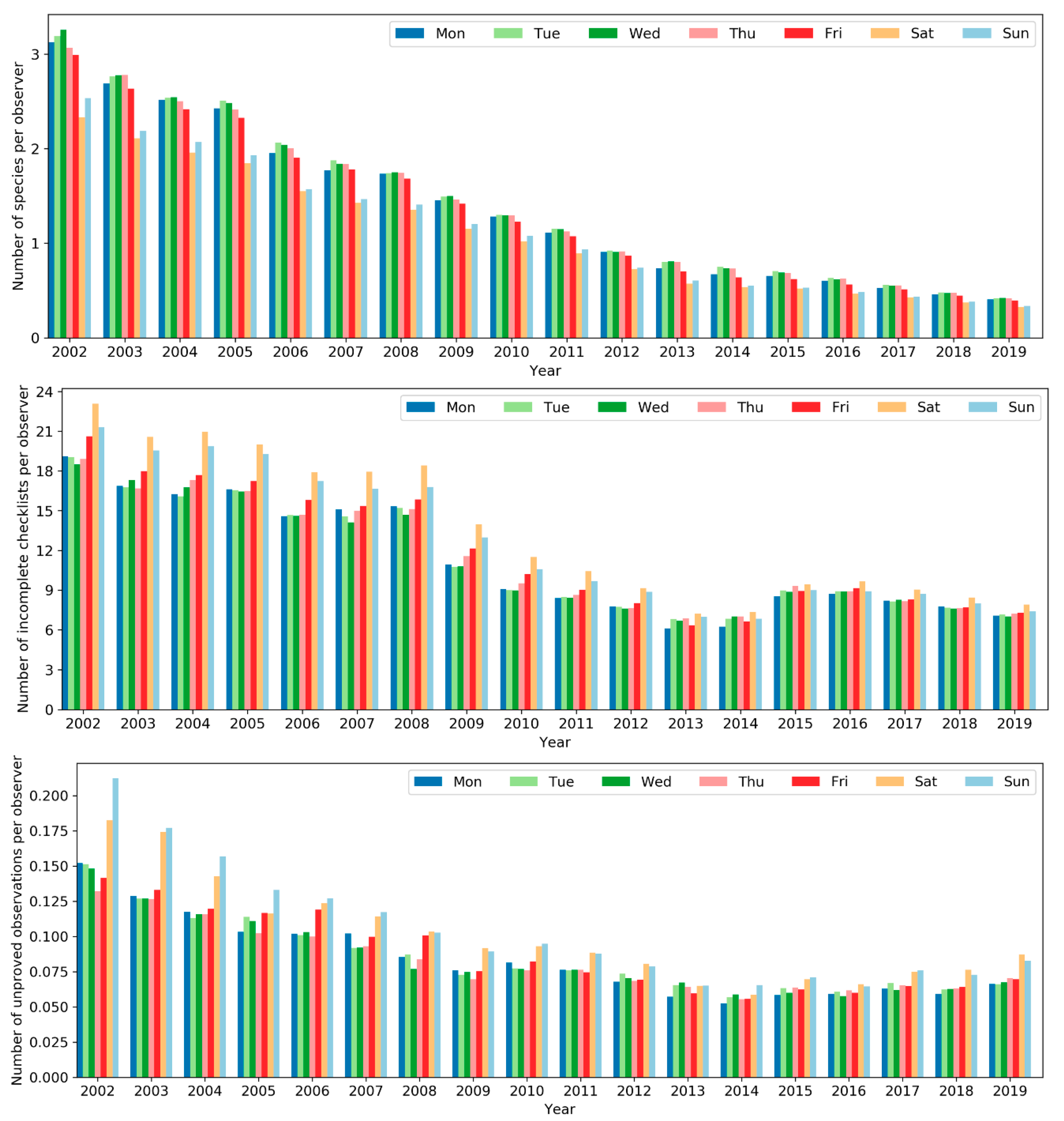
However, the level of expertise of the birders who were active on weekends and the quality of their data submissions was notably different from those active on weekdays (Figure 22). The average number of species per observer, an indicator of the level of birding expertise, was lower among birders active on weekends. Moreover, the number of incomplete checklists (i.e., not all species were identified and reported) and unapproved observations per observer, two indicators of data quality, were both higher among birders active on weekends. The evidence suggests birders who were active on weekdays were of an overall higher level of expertise and data contributed by them were of higher quality. This might be due to the fac that a larger number of novice birders tend to go birding only on weekends while expert birder may conduct birding on weekdays besides weekends.
4.3. Biases in VGI and Their Implications
Several forms of biases exist in VGI due to the characteristics of volunteer data contribution activities. When utilizing VGI, one should assess the fitness of use of VGI in the context of particular applications by examining the extent of the biases, their potential impacts, and possible methods to account for the biases.
4.3.1. Spatial Bias
Spatial bias is often intrinsic to the sampling efforts of volunteer data contributors. Unlike traditional geographic sampling where sampling locations are designed following a certain spatial sampling scheme (e.g., stratified random sampling), individual volunteers choose sampling locations (i.e., where to conduct observations) largely at their own will in ad hoc or opportunistic manners, without coordinating sampling efforts with other volunteers [18]. As a result, volunteer sampling efforts often concentrate in more accessible areas (Figure 4) and such sampling efforts are subject to spatial bias. In some cases, volunteers do make their decisions regarding where to sample based on where others have sampled. For example, eBird contributors may consult the “hotspots” map and species distribution maps provided by eBird [34] and accordingly select “hotspots” (areas with larger number of reported bird species) for birding. This, however, may reinforce existing spatial bias in sampling efforts, as areas with higher sampling intensity get sampled repeatedly (over-sampled) while areas with lower sampling intensity remain under-sampled.
Geographic data contributed by volunteers, when using geographic samples for analysis and modeling, need to be representative so properties of the underlying population can be inferred from the sample with satisfactory accuracy. The representativeness of geographic samples collected through traditional spatial sampling protocols is often ensured by following a rigorous sampling scheme such that sampling locations properly cover the environmental gradients in the geographic area of interest [63]. However, due to spatial bias in volunteer sampling efforts, the sampling locations may not have a good coverage over the environmental gradients, which impedes the representativeness of volunteer-contributed geographic samples [64]. For instance, more occurrence locations of a bird species in urban areas as reflected in the eBird database do not necessarily mean the species actually prefer urban habitats; it may be that there were simply not sufficient sampling efforts in non-urban habitats to discover the species. When the occurrence locations are used to predict species distribution, e.g., through species distribution modeling, such spatial bias needs to be accounted for in order to improve modeling and prediction accuracy [8,16,17,55,65,66,67].
4.3.2. Temporal Bias
Temporal bias also exists in volunteer sampling efforts, potentially at multiple temporal granularities. As profiling of the eBird data shows, sampling efforts and reported bird species are increasing over the years, with significant monthly fluctuations and notably more contributions on weekends. When observations from VGI are used to analyze temporal changes of geographic phenomena, such temporal bias should be accounted for [15]. For instance, the increasing number of bird species reported to eBird (Figure 16) does not mean increasing bird diversity on Earth. The increase is basically attributed to the increase in sampling efforts. As another example, although in the northern hemisphere there are a larger number of bird species reported to eBird in May than in September, one cannot definitively conclude that more bird species are present in May; there are simply not as many sampling efforts in September, and thus, the comparison would not be meaningful without disentangling the effects of the uneven sampling efforts. In fact, when eBird observations are used for modeling and predicting species geographic distribution, temporal variations in sampling efforts are often controlled for by selecting only observations within certain periods of roughly uniform sampling efforts [8,17].
4.3.3. Contributor Bias
Volunteer contributors are of various levels of skill in contributing data, and skill level of the same contributor may change over time. For example, the varied levels of expertise among eBird contributors may well be reflected in the number of active days they report observations (Figure 13) and in the number of reported sampling events, sampling locations and bird species (Figure 14). Many observers are ephemeral one-time contributors submitting only a single record. Only a small portion of the contributor are experts who tend to actively contribute large quantities of data over the long term [51]. In fact, when counting birds, there exist both between-observer differences [68] and within-observer differences (i.e., a change in ability to count birds of a given species after an observer’s first year experience) [69].
Such observer bias may need to be accounted for when using VGI data in analyses. For instance, [70] reveal that for low-density populations, using data contributed by novice and experienced observers together may lead to erroneous site occupancy models. Other studies have found that observation skills of volunteer contributors can be estimated using species accumulation curves [71] and incorporating observer quality as a covariable to account for observer differences [68]; removing an observer’s first year of observation [69] improves population trends estimation, and incorporating estimates of observer expertise in occupancy model improves species distributions from citizen science data [72].
4.3.4. Observation Bias
Bias also exists regarding the observation target. While some targets are easy to observe and identify, others may be more challenging. As a result, volunteer observations may be biased towards the easy targets in data volume. Common species may be reported repeatedly in many sampling events and by many observers, while only few records of rare and elusive species may be reported. Another complication is that observers may have their respective preferences on what to observe and report. Expert birders may be only interested in reporting rare species while ignoring common species. Such observation bias in VGI may deserve treatment in certain VGI applications. In fact, eBird let users report whether a checklist (i.e., sampling event) includes all species they could detect and identify (“complete” checklist). This makes it possible to filter the checklists to use only complete ones in analysis and modeling and thus enables analysts to move away from the reporting preference issue mentioned above [73]. eBird encourages observers to submit complete checklists, and a high proportion (~75%) of the submitted checklists in eBird database are complete.
5. Conclusions
Using eBird as an example, this study explores spatial and temporal patterns in volunteer data contribution activities. The sampling efforts of eBird contributors are biased in space and time. Most sampling efforts are concentrated in areas of denser populations and/or better accessibility, with the most intensively sampled areas being in proximity to big cities in developed regions of the world. Due to the spatially biased sampling efforts, reported bird species are also spatially biased towards areas where more sampling efforts occur. Temporally, eBird sampling efforts and reported bird species are increasing over the years, with significant monthly fluctuations and notably more data reported on weekends. Such trends are driven by continued development of the eBird project and by characteristics of both the bird species (e.g., breeding season) and the observers (e.g., more birding on weekends). Other forms of biases also exist in volunteer data contribution activities (e.g., contributor bias, observation bias). The fitness of use of VGI in the context of particular applications should be evaluated by examining the extent of the spatial, temporal and other biases and their potential impacts. In many cases, the biases need to be accounted for such that reliable inferences can be made from VGI observations.
Funding
This research was funded by Microsoft AI for Earth—Azure Compute Credit Grants.
Acknowledgments
This study was supported by the Faculty Start-up Funds and the Faculty Research Fund at the University of Denver. The author thanks the many eBird contributors for their efforts of contributing birding records to eBird, the Cornell Lab of Ornithology for making eBird data open and freely available, and Alison Johnston (Research Associate at eBird) and the anonymous reviewers for their constructive comments that helped improve this manuscript.
Conflicts of Interest
The authors declare no conflict of interest.
References
- Goodchild, M.F. Citizens as sensors: The world of volunteered geography. GeoJournal 2007, 69, 211–221. [Google Scholar] [CrossRef]
- Haklay, M.; Weber, P. OpenStreetMap: User-generated street maps. IEEE Pervasive Comput. 2008, 7, 12–18. [Google Scholar] [CrossRef]
- Sullivan, B.L.; Wood, C.L.; Iliff, M.J.; Bonney, R.E.; Fink, D.; Kelling, S. eBird: A citizen-based bird observation network in the biological sciences. Biol. Conserv. 2009, 142, 2282–2292. [Google Scholar] [CrossRef]
- Wood, C.; Sullivan, B.; Iliff, M.; Fink, D.; Kelling, S. eBird: Engaging birders in science and conservation. PLoS Biol. 2011, 9, e1001220. [Google Scholar] [CrossRef] [PubMed]
- Arsanjani, J.J.; Zipf, A.; Mooney, P.; Helbich, M. OpenStreetMap in GIScience: Experiences, Research, and Applications; Springer: Berlin/Heidelberg, Germany, 2015; ISBN 3319142801. [Google Scholar]
- Sullivan, B.L.; Aycrigg, J.L.; Barry, J.H.; Bonney, R.E.; Bruns, N.; Cooper, C.B.; Damoulas, T.; Dhondt, A.A.; Dietterich, T.; Farnsworth, A.; et al. The eBird enterprise: An integrated approach to development and application of citizen science. Biol. Conserv. 2014, 169, 31–40. [Google Scholar] [CrossRef]
- Sachdeva, S.; McCaffrey, S.; Locke, D. Social media approaches to modeling wildfire smoke dispersion: Spatiotemporal and social scientific investigations. Inf. Commun. Soc. 2017, 20, 1146–1161. [Google Scholar] [CrossRef]
- Fink, D.; Hochachka, W.M.; Zuckerberg, B.; Winkler, D.W.; Shaby, B.; Munson, M.A.; Hooker, G.; Riedewald, M.; Sheldon, D.; Kelling, S. Spatiotemporal exploratory models for broad-scale survey data. Ecol. Appl. 2010, 20, 2131–2147. [Google Scholar] [CrossRef] [PubMed]
- Malik, M.M.; Lamba, H.; Nakos, C.; Pfeffer, J. Population Bias in Geotagged Tweets. In Proceedings of the Nineth International AAAI Conference on Web and Social Media, Oxford, UK, 26–29 May 2015; pp. 18–27. [Google Scholar]
- Brown, G. A review of sampling effects and response bias in Internet participatory mapping (PPGIS/PGIS/VGI). Trans. GIS 2017, 21, 39–56. [Google Scholar] [CrossRef]
- Hecht, B.; Stephens, M. A tale of cities: Urban biases in volunteered geographic information. In Proceedings of the Eighth International Conference on Web and Social Media (ICWSM), Ann Arbor, MI, USA, 1–4 June 2014; pp. 197–205. [Google Scholar]
- Zhang, Y.; Li, X.; Wang, A.; Bao, T.; Tian, S. Density and diversity of OpenStreetMap road networks in China. J. Urban Manag. 2015, 4, 135–146. [Google Scholar] [CrossRef]
- Yang, A.; Fan, H.; Jing, N.; Sun, Y.; Zipf, A. Temporal Analysis on Contribution Inequality in OpenStreetMap: A Comparative Study for Four Countries. ISPRS Int. J. Geo-Inf. 2016, 5, 5. [Google Scholar] [CrossRef]
- Basiri, A.; Haklay, M.; Foody, G.; Mooney, P. Crowdsourced geospatial data quality: Challenges and future directions. Int. J. Geogr. Inf. Sci. 2019, 33, 1588–1593. [Google Scholar] [CrossRef]
- Boakes, E.H.; McGowan, P.J.K.; Fuller, R.A.; Ding, C.; Clark, N.E.; O’Connor, K.; Mace, G.M. Distorted views of biodiversity: Spatial and temporal bias in species occurrence data. PLoS Biol. 2010, 8, e1000385. [Google Scholar] [CrossRef] [PubMed]
- Zhang, G. Enhancing VGI application semantics by accounting for spatial bias. Big Earth Data 2019, 3, 255–268. [Google Scholar] [CrossRef]
- Zhang, G.; Zhu, A.-X. A representativeness directed approach to spatial bias mitigation in VGI for predictive mapping. Int. J. Geogr. Inf. Sci. 2019, 33, 1873–1893. [Google Scholar] [CrossRef]
- Zhu, A.-X.; Zhang, G.; Wang, W.; Xiao, W.; Huang, Z.-P.; Dunzhu, G.-S.; Ren, G.; Qin, C.-Z.; Yang, L.; Pei, T.; et al. A citizen data-based approach to predictive mapping of spatial variation of natural phenomena. Int. J. Geogr. Inf. Sci. 2015, 29, 1864–1886. [Google Scholar] [CrossRef]
- Boakes, E.H.; Gliozzo, G.; Seymour, V.; Harvey, M.; Smith, C.; Roy, D.B.; Haklay, M. Patterns of contribution to citizen science biodiversity projects increase understanding of volunteers’ recording behaviour. Sci. Rep. 2016, 6, 1–11. [Google Scholar] [CrossRef] [PubMed]
- Antoniou, V.; Skopeliti, A. Measures and indicators of VGI quality: An overview. ISPRS Ann. Photogramm. Remote Sens. Spat. Inf. Sci. 2015, II-3/W5, 345–351. [Google Scholar] [CrossRef]
- Sauermanna, H.; Franzonib, C. Crowd science user contribution patterns and their implications. Proc. Natl. Acad. Sci. USA 2015, 112, 679–684. [Google Scholar] [CrossRef]
- Neis, P.; Zipf, A. Analyzing the contributor activity of a volunteered geographic information project-The case of OpenStreetMap. ISPRS Int. J. Geo-Inf. 2012, 1, 146–165. [Google Scholar] [CrossRef]
- Li, L.; Goodchild, M.F.; Xu, B. Spatial, temporal, and socioeconomic patterns in the use of Twitter and Flickr. Cartogr. Geogr. Inf. Sci. 2013, 40, 61–77. [Google Scholar] [CrossRef]
- Nielsen, J. The 90-9-1 Rule for Participation Inequality in Social Media and Online Communities. 2006. Available online: https://www.nngroup.com/articles/participation-inequality (accessed on 1 October 2020).
- Haklay, M.E. Why is Participation Inequality Important? Ubiquity Press: London, UK, 2016. [Google Scholar]
- Carron-Arthur, B.; Cunningham, J.A.; Griffiths, K.M. Describing the distribution of engagement in an Internet support group by post frequency: A comparison of the 90-9-1 Principle and Zipf’s Law. Internet Interv. 2014, 1, 165–168. [Google Scholar] [CrossRef]
- Girres, J.-F.; Touya, G. Quality assessment of the French OpenStreetMap dataset. Trans. GIS 2010, 14, 435–459. [Google Scholar] [CrossRef]
- Bittner, C. Diversity in volunteered geographic information: Comparing OpenStreetMap and Wikimapia in Jerusalem. GeoJournal 2017, 82, 887–906. [Google Scholar] [CrossRef]
- Geldmann, J.; Heilmann-Clausen, J.; Holm, T.E.; Levinsky, I.; Markussen, B.; Olsen, K.; Rahbek, C.; Tøttrup, A.P. What determines spatial bias in citizen science? Exploring four recording schemes with different proficiency requirements. Divers. Distrib. 2016, 22, 1139–1149. [Google Scholar] [CrossRef]
- Audubon. Cornell Lab of Orithnology about eBird. Available online: https://ebird.org/about (accessed on 17 September 2019).
- eBird. eBird Basic Dataset Metadata (v1.12). 2019. Available online: https://ebird.org/science/download-ebird-data-products (accessed on 17 September 2019).
- Kelling, S.; Lagoze, C.; Wong, W.-K.; Yu, J.; Damoulas, T.; Gerbracht, J.; Fink, D.; Gomes, C. eBird: A Human/Computer Learning Network to Improve Biodiversity Conservation and Research. AI Mag. 2013, 34, 10–20. [Google Scholar] [CrossRef]
- La Sorte, F.A.; Somveille, M. Survey completeness of a global citizen-science database of bird occurrence. Ecography 2020, 43, 34–43. [Google Scholar] [CrossRef]
- eBird. Explore Hotspots-eBird. Available online: https://ebird.org/hotspots (accessed on 17 September 2019).
- UNDP. Human Development Indices and Indicators: 2018 Statistical Update; UNDP: New York, NY, USA, 2018. [Google Scholar]
- USFWS. Birding in the United States: A Demographic and Economic Analysis Addendum to the 2011 National Survey of Fishing, Hunting, and Wildlife-Associated Recreation; U.S. Fish and Wildlife Service: Washington, DC, USA, 2013. Available online: https://digitalmedia.fws.gov/digital/collection/document/id/1874/ (accessed on 1 October 2020).
- eBird. Mobile Now Available in 5 Languages. Available online: https://ebird.org/news/mobiletranslation/ (accessed on 20 March 2020).
- Tuanmu, M.N.; Jetz, W. A global 1-km consensus land-cover product for biodiversity and ecosystem modelling. Glob. Ecol. Biogeogr. 2014, 23, 1031–1045. [Google Scholar] [CrossRef]
- Global 1-km Consensus Land Cover. Available online: http://www.earthenv.org/landcover (accessed on 15 June 2020).
- Center for International Earth Science Information Network—CIESIN—Columbia University. Gridded Population of the World, Version 4 (GPWv4): Population Density, Revision 11. 2018. Available online: https://data.nasa.gov/dataset/Gridded-Population-of-the-World-Version-4-GPWv4-Po/w4yu-b8bh (accessed on 15 June 2020).
- Population Density, v4.11 (2000, 2005, 2010, 2015, 2020). Available online: https://sedac.ciesin.columbia.edu/data/set/gpw-v4-population-density-rev11 (accessed on 15 June 2020).
- Meijer, J.R.; Huijbregts, M.A.J.; Schotten, K.C.G.J.; Schipper, A.M. Global patterns of current and future road infrastructure. Environ. Res. Lett. 2018, 13, 064006. [Google Scholar] [CrossRef]
- GRIP Global Roads Database. Available online: https://www.globio.info/download-grip-dataset (accessed on 15 June 2020).
- Human Development Data (1990–2018). Available online: http://hdr.undp.org/en/data (accessed on 1 October 2020).
- An Overview of All the Official Languages Spoken per Country. Available online: http://www.arcgis.com/home/item.html?id=5c6ec52c374249a781aede5802994c95 (accessed on 15 June 2020).
- 2020 World Population by Country. Available online: https://worldpopulationreview.com/ (accessed on 15 June 2020).
- Phillips, S.J.; Anderson, R.P.; Schapire, R.E. Maximum entropy modeling of species geographic distributions. Ecol. Model. 2006, 190, 231–259. [Google Scholar] [CrossRef]
- Yan, Y.; Kuo, C.; Feng, C.; Huang, W.; Fan, H. Coupling maximum entropy modeling with geotagged social media data to determine the geographic distribution of tourists. Int. J. Geogr. Inf. Sci. 2018, 32, 1699–1736. [Google Scholar] [CrossRef]
- Phillips, S.J.; Dudík, M.; Schapire, R.E. Maxent Software for Modeling Species Niches and Distributions, (Version 3.4.1). 2019. Available online: https://biodiversityinformatics.amnh.org/open_source/maxent (accessed on 1 March 2019).
- Phillips, S.J.; Dudík, M. Modeling of species distributions with Maxent: New extensions and a comprehensive evaluation. Ecography 2008, 31, 161–175. [Google Scholar] [CrossRef]
- Bégin, D.; Devillers, R.; Roche, S. The life cycle of contributors in collaborative online communities-the case of OpenStreetMap. Int. J. Geogr. Inf. Sci. 2018, 32, 1611–1630. [Google Scholar] [CrossRef]
- Welcome to ornitho.ch. Available online: https://www.ornitho.ch/ (accessed on 1 October 2020).
- iNaturalist. Available online: https://www.inaturalist.org/ (accessed on 1 October 2020).
- Conflict Is Still Africa’s Biggest Challenge in 2020. Available online: https://reliefweb.int/report/world/conflict-still-africa-s-biggest-challenge-2020 (accessed on 1 October 2020).
- Johnston, A.; Moran, N.; Musgrove, A.; Fink, D.; Baillie, S.R. Estimating species distributions from spatially biased citizen science data. Ecol. Model. 2020, 422, 108927. [Google Scholar] [CrossRef]
- Newman, G.; Graham, J.; Crall, A.; Laituri, M. The art and science of multi-scale citizen science support. Ecol. Inform. 2011, 6, 217–227. [Google Scholar] [CrossRef]
- Wikipedia eBird. Available online: https://en.wikipedia.org/wiki/EBird (accessed on 17 July 2020).
- eBird Mobile App for iOS Now Available! Available online: https://ebird.org/news/ebird_mobile_ios1 (accessed on 1 October 2020).
- Cornell Lab of Orinithology Merlin. Available online: https://merlin.allaboutbirds.org/the-story/ (accessed on 21 July 2020).
- Great (Global) Backyard Bird Count This Weekend! Available online: https://ebird.org/news/great-global-backyard-bird-count-this-weekend/ (accessed on 3 October 2020).
- Global Big Day—9 May 2020. Available online: https://ebird.org/news/global-big-day-9-may-2020 (accessed on 21 July 2020).
- October Big Day—19 October 2019. Available online: https://ebird.org/news/october-big-day-19-october-2019 (accessed on 21 July 2020).
- Jensen, R.R.; Shumway, J.M. Sampling our world. In Research Methods in Geography: A Critical Introduction; Gomez, B., Jones, J.P., III, Eds.; John Wiley & Sons: Hoboken, NJ, USA, 2010; pp. 77–90. [Google Scholar]
- Zhang, G.; Zhu, A.-X. The representativeness and spatial bias of volunteered geographic information: A review. Ann. GIS 2018, 24, 151–162. [Google Scholar] [CrossRef]
- Pardo, I.; Pata, M.P.; Gómez, D.; García, M.B. A novel method to handle the effect of uneven sampling effort in biodiversity databases. PLoS ONE 2013, 8, e52786. [Google Scholar] [CrossRef]
- Stolar, J.; Nielsen, S.E. Accounting for spatially biased sampling effort in presence-only species distribution modelling. Divers. Distrib. 2015, 21, 595–608. [Google Scholar] [CrossRef]
- Robinson, O.J.; Ruiz-Gutierrez, V.; Fink, D. Correcting for bias in distribution modelling for rare species using citizen science data. Divers. Distrib. 2018, 24, 460–472. [Google Scholar] [CrossRef]
- Sauer, J.R.; Peterjohn, B.G.; Link, W.A. Observer differences in the North American Breeding Bird Survey. Auk 1994, 111, 50–62. [Google Scholar] [CrossRef]
- Kendall, W.L.; Peterjohn, B.G.; Sauer, J.R.; Url, S. First-time observer effects in the North American Breeding Bird Survey. Auk 1996, 113, 823–829. [Google Scholar] [CrossRef]
- Fitzpatrick, M.C.; Preisser, E.L.; Ellison, A.M.; Elkinton, J.S. Observer bias and the detection of low-density populations. Ecol. Appl. 2009, 19, 1673–1679. [Google Scholar] [CrossRef] [PubMed]
- Kelling, S.; Johnston, A.; Hochachka, W.M.; Iliff, M.; Fink, D.; Gerbracht, J.; Lagoze, C.; La Sorte, F.A.; Moore, T.; Wiggins, A.; et al. Can Observation Skills of Citizen Scientists Be Estimated Using Species Accumulation Curves? PLoS ONE 2015, 10, e0139600. [Google Scholar] [CrossRef] [PubMed]
- Johnston, A.; Fink, D.; Hochachka, W.M.; Kelling, S. Estimates of observer expertise improve species distributions from citizen science data. Methods Ecol. Evol. 2018, 9, 88–97. [Google Scholar] [CrossRef]
- Johnston, A.; Hochachka, W.; Strimas-Mackey, M.; Ruiz Gutierrez, V.; Robinson, O.; Auer, T.; Kelling, S.; Fink, D. Analytical guidelines to increase the value of citizen science data: Using eBird data to estimate species occurrence. bioRxiv 2020. Available online: https://www.biorxiv.org/content/10.1101/574392v3.full.pdf (accessed on 15 June 2020).
Figure 1.
Spatial distribution of eBird sampling locations in 2019.

Figure 2.
Covariates used for modeling the spatial pattern in sampling efforts of eBird contributors.
Figure 2.
Covariates used for modeling the spatial pattern in sampling efforts of eBird contributors.
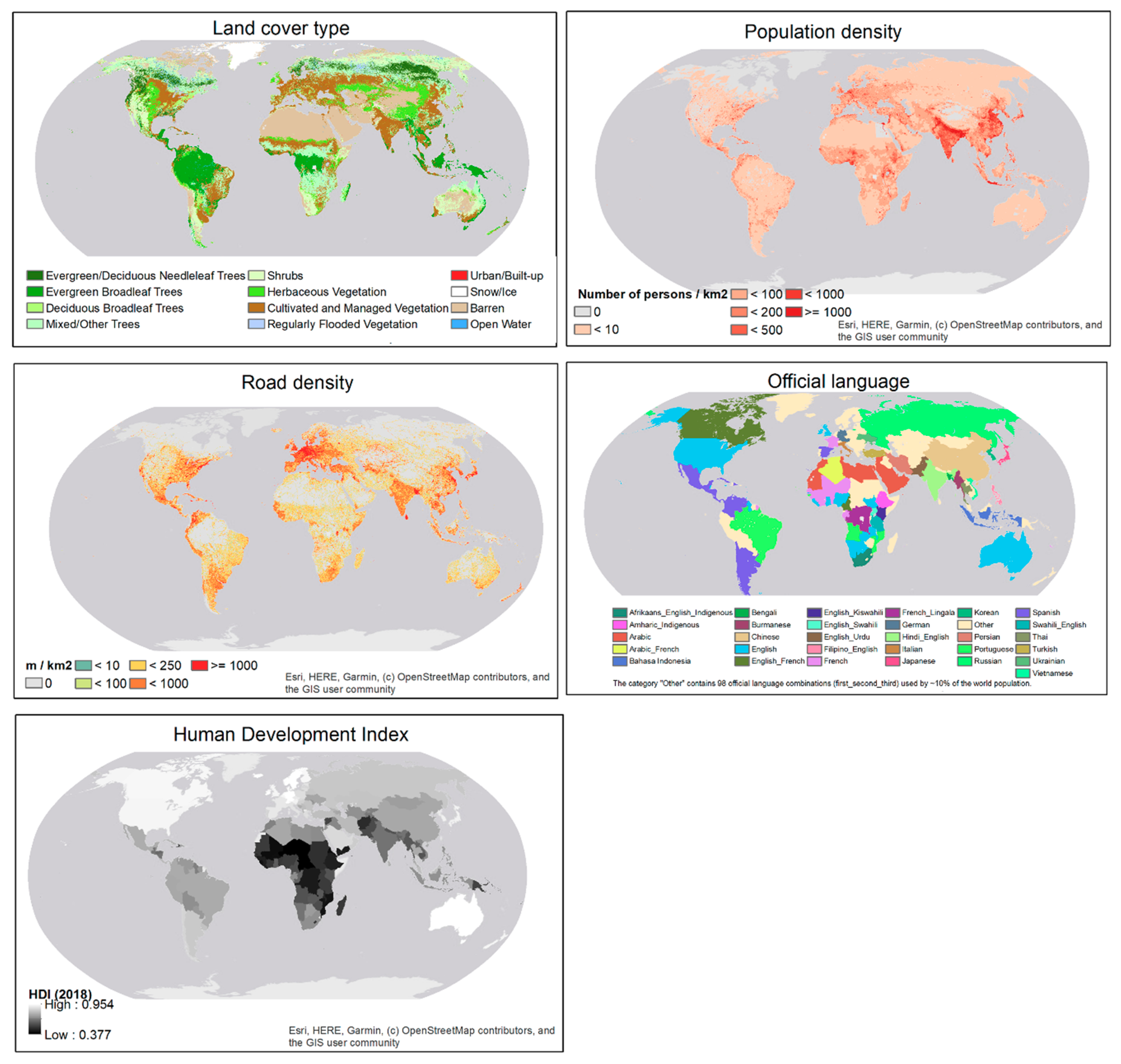
Figure 3.
Frequency distribution of sampling locations and of the world on the covariates.
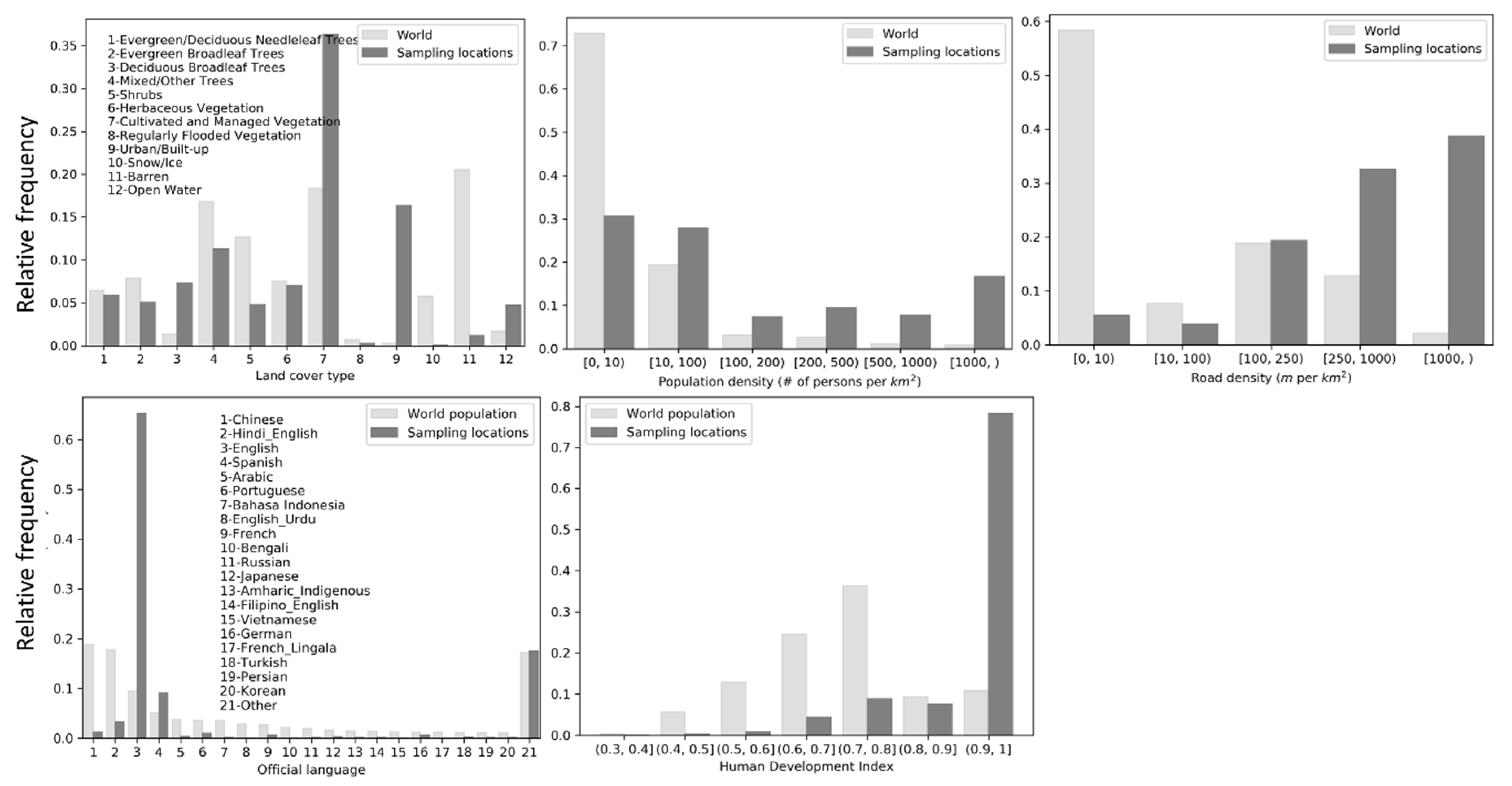
Figure 4.
The number of cumulative eBird sampling events as of 31 December 2019 mapped over 0.25° latitude × 0.25° longitude grid cells. Intervals were determined loosely following quartile classification method.
Figure 4.
The number of cumulative eBird sampling events as of 31 December 2019 mapped over 0.25° latitude × 0.25° longitude grid cells. Intervals were determined loosely following quartile classification method.

Figure 5.
Number of sampling events in each year (2002–2019).

Figure 6.
Percentage of sampling events in each month relative to the yearly total number of events.
Figure 6.
Percentage of sampling events in each month relative to the yearly total number of events.
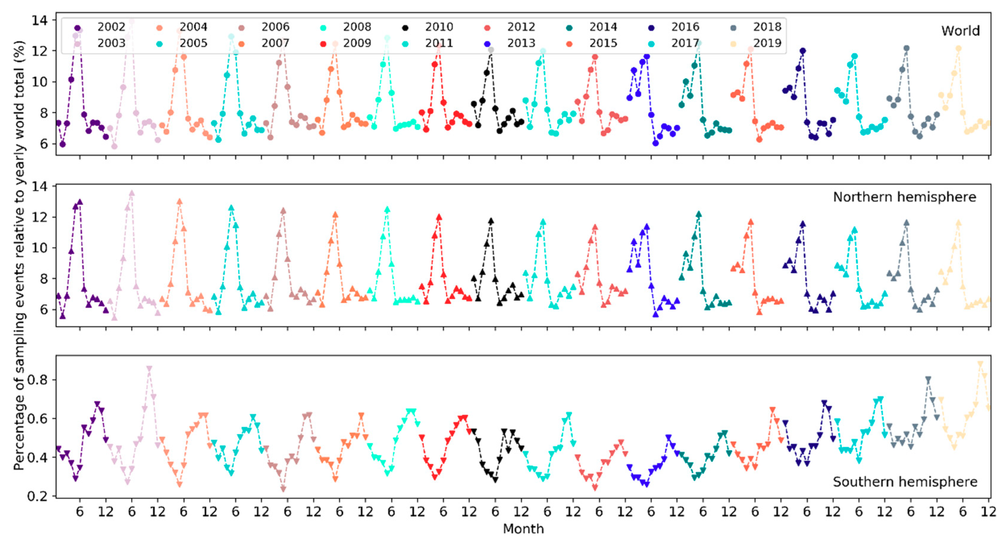
Figure 7.
Average number of sampling events on each day of the week over the years.

Figure 8.
Frequency distribution of sampling events by the number of reported species.
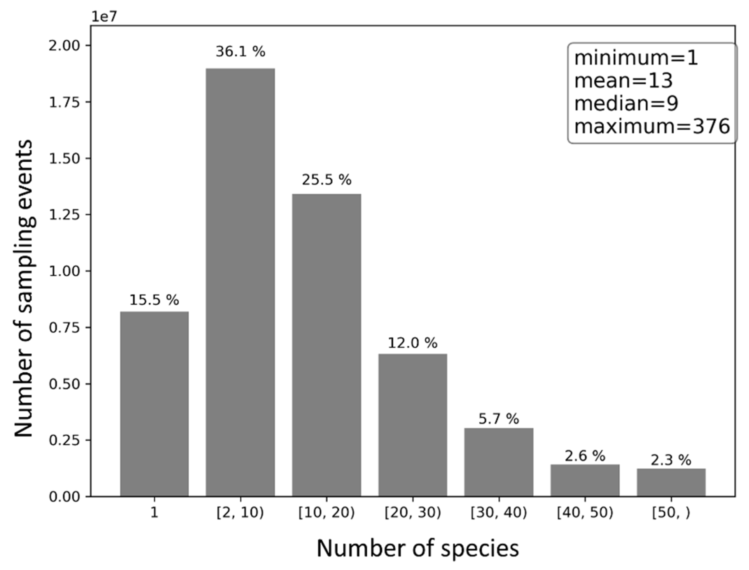
Figure 9.
The cumulative number of observers as of 31 December 2019 mapped over 0.25° latitude × 0.25° longitude grid cells. Intervals were determined loosely following quartile classification method.
Figure 9.
The cumulative number of observers as of 31 December 2019 mapped over 0.25° latitude × 0.25° longitude grid cells. Intervals were determined loosely following quartile classification method.
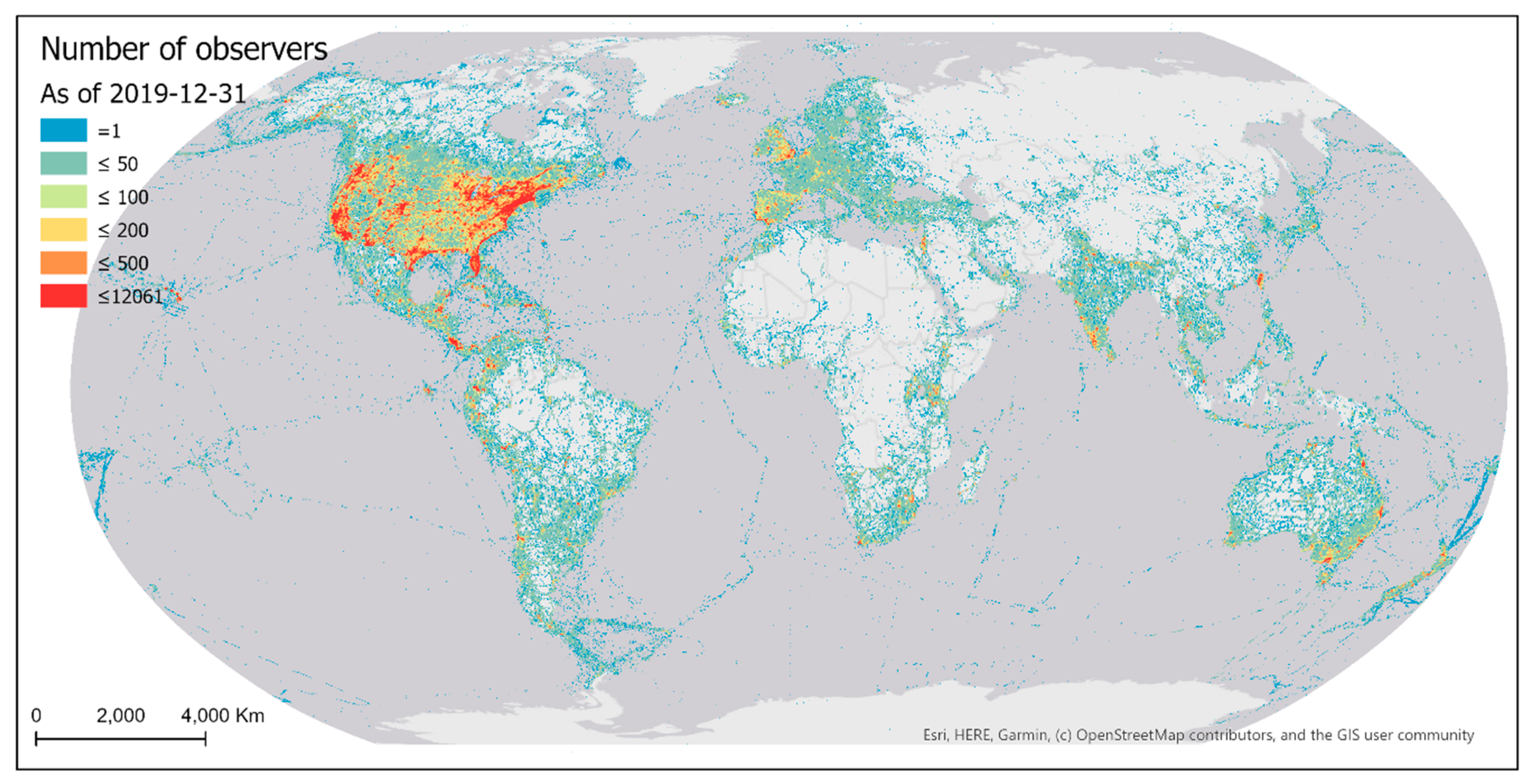
Figure 10.
Number of active observers in each year (2002–2019).
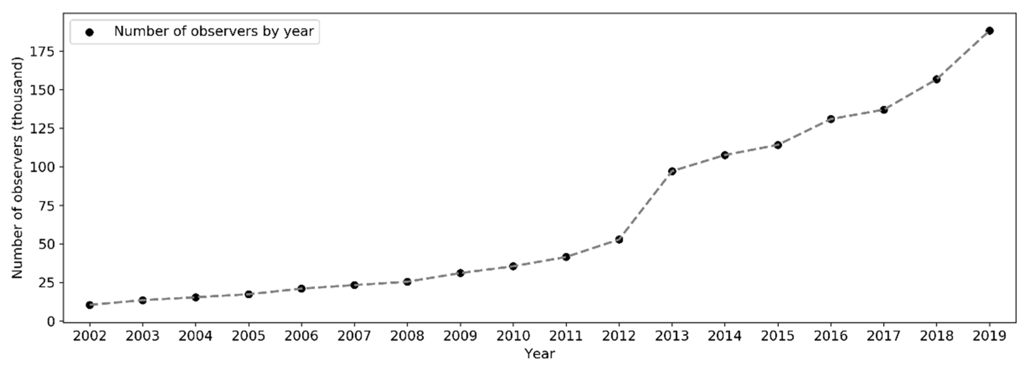
Figure 11.
Percentage of observers in each month relative to the yearly total number of observers.
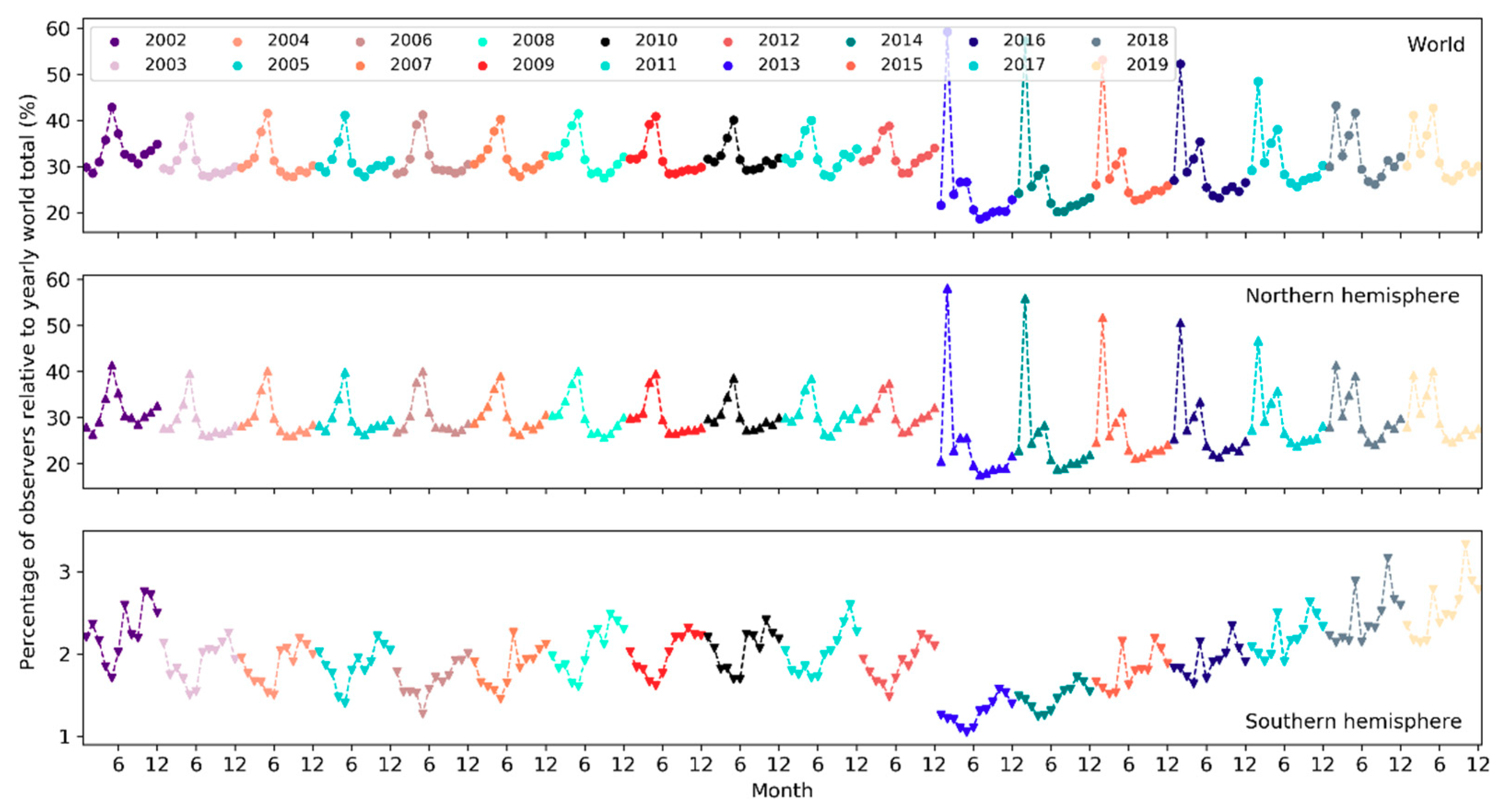
Figure 12.
Average number of active observers on each day of the week over the years.
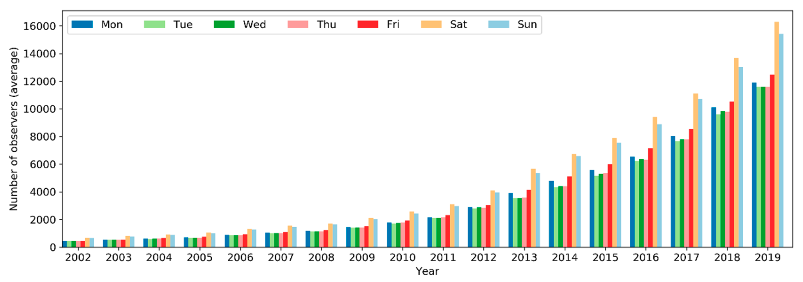
Figure 13.
Frequency distribution of observers by year of first observation (upper left), year of last observation (upper right), number of years between the first and last observations (lower left), and number of active dates (lower right).
Figure 13.
Frequency distribution of observers by year of first observation (upper left), year of last observation (upper right), number of years between the first and last observations (lower left), and number of active dates (lower right).

Figure 14.
Frequency distribution of observers by number of reported species (left), number of sampling events (center) and number of sampling locations (right).
Figure 14.
Frequency distribution of observers by number of reported species (left), number of sampling events (center) and number of sampling locations (right).

Figure 15.
The cumulative number of species reported to eBird as of 31 December 2019 mapped over 0.25° latitude × 0.25° longitude grid cells. Intervals were determined loosely following quartile classification method.
Figure 15.
The cumulative number of species reported to eBird as of 31 December 2019 mapped over 0.25° latitude × 0.25° longitude grid cells. Intervals were determined loosely following quartile classification method.
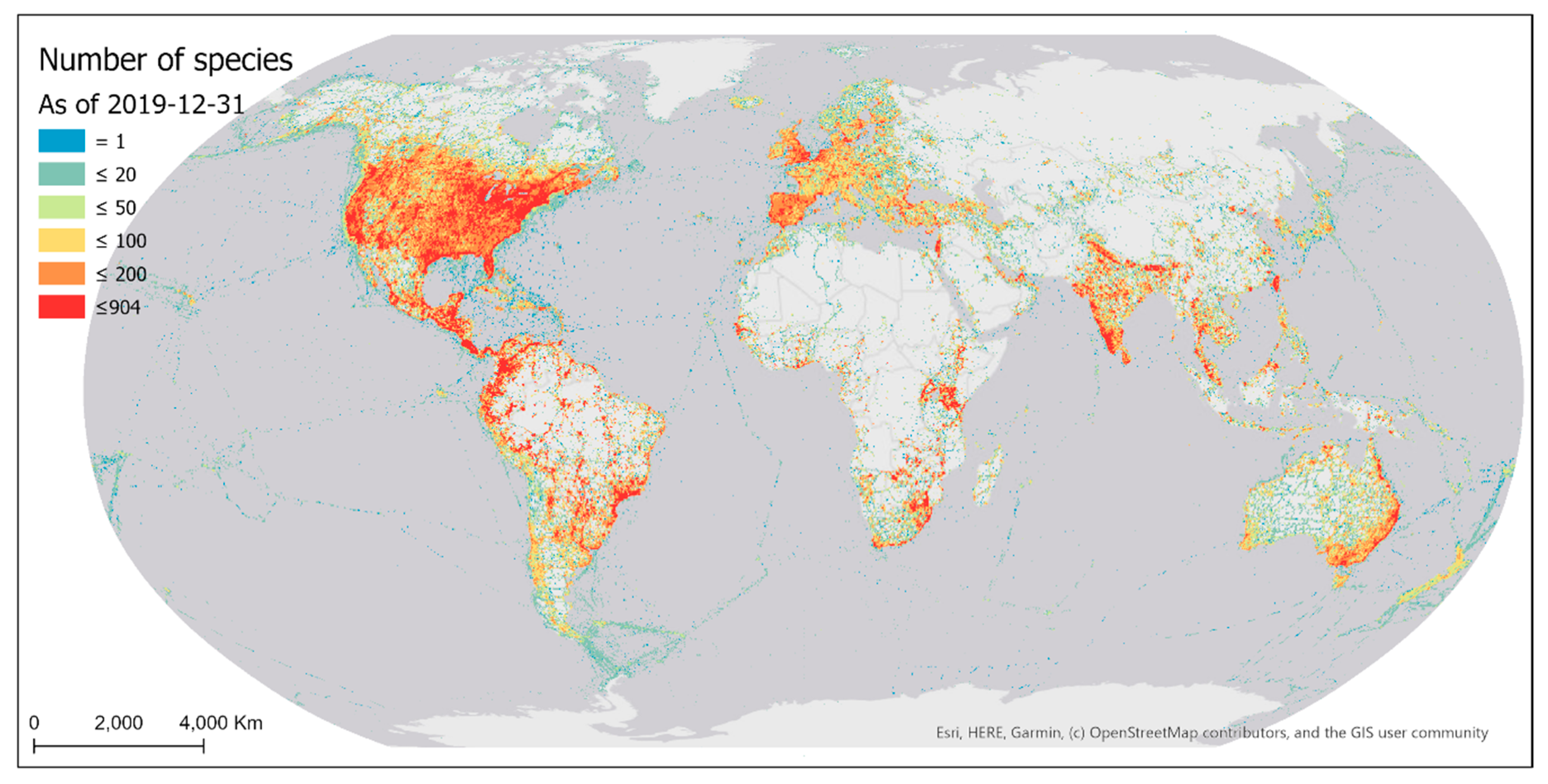
Figure 16.
Number of species reported in each year (2002–2019).

Figure 17.
Percentage of species reported in each month relative to the yearly total number of species.
Figure 17.
Percentage of species reported in each month relative to the yearly total number of species.

Figure 18.
Average number of species reported on each day of the week over the years.
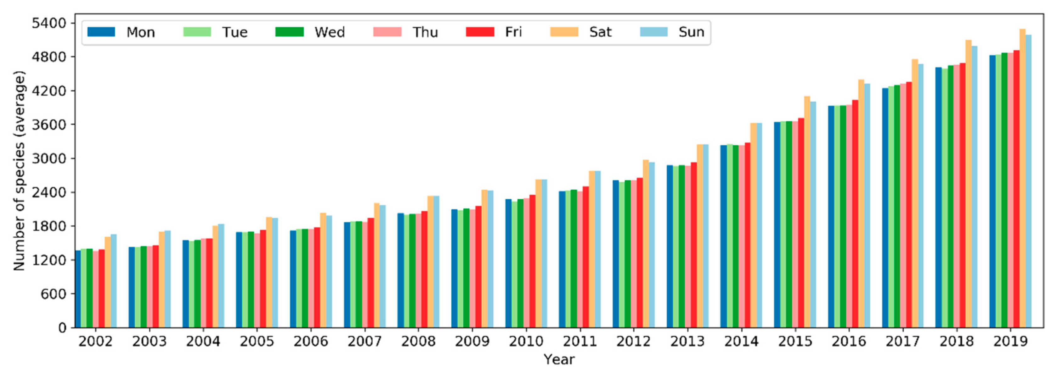
Figure 19.
Distribution of the number of species by the number of observers who reported the same bird species (left) and by the number of sampling events in which the same species was reported (right).
Figure 19.
Distribution of the number of species by the number of observers who reported the same bird species (left) and by the number of sampling events in which the same species was reported (right).

Figure 20.
Jackknife test of variable importance to the Maxent model based on test AUC.

Figure 21.
Map of sampling probability of eBird contributors modeled and predicted using Maxent.
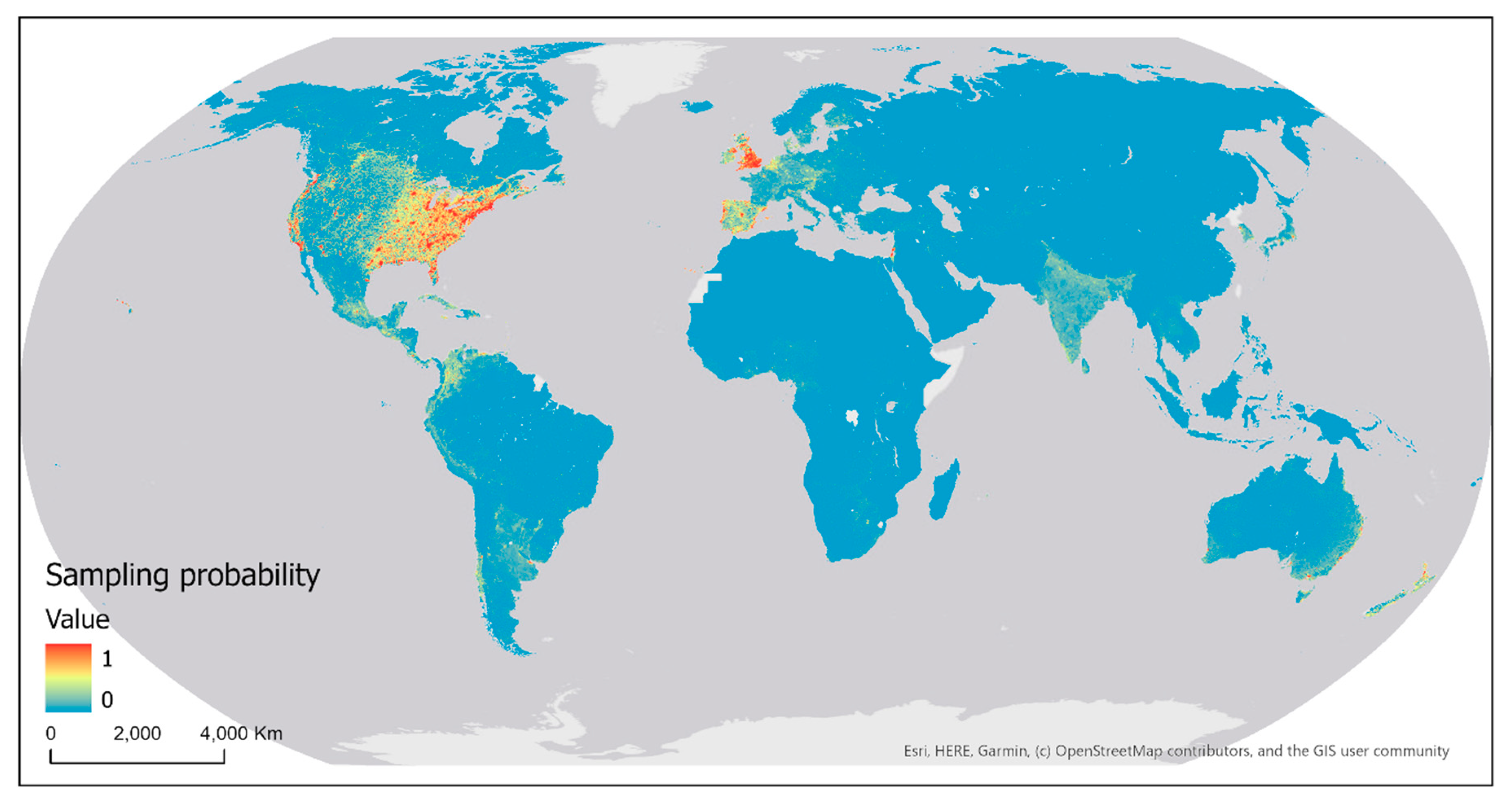
Figure 22.
Number of species (top), incomplete checklists (center), and unapproved observations (bottom) per observer across the days of the week.
Figure 22.
Number of species (top), incomplete checklists (center), and unapproved observations (bottom) per observer across the days of the week.


Table 1.
Top 10 countries and territories most intensively sampled by eBird contributors.
| Country/Territory | Sampling Events | Sampling Locations | Observers | Species | ||
|---|---|---|---|---|---|---|
| n | % | n | % | |||
| United States | 36,540,720 | 67.9% | 5,166,510 | 61.6% | 417,288 | 1444 |
| Canada | 6,304,830 | 11.7% | 915,075 | 10.9% | 59,733 | 761 |
| Australia | 1,392,746 | 2.6% | 218,756 | 2.6% | 11,176 | 876 |
| India | 1,005,541 | 1.9% | 219,430 | 2.6% | 18,824 | 1536 |
| Spain | 757,638 | 1.4% | 148,401 | 1.8% | 9484 | 687 |
| United Kingdom | 714,712 | 1.3% | 123,621 | 1.5% | 11,898 | 756 |
| Mexico | 488,476 | 0.9% | 108,411 | 1.3% | 15,813 | 1140 |
| Taiwan | 453,852 | 0.8% | 75,321 | 0.9% | 3421 | 742 |
| Costa Rica | 383,191 | 0.7% | 68,171 | 0.8% | 12,855 | 930 |
| Portugal | 369,303 | 0.7% | 59,118 | 0.7% | 4170 | 620 |
Table 2.
Relative contributions of the environmental and cultural variables to the Maxent model.
| Variable | Percent Contribution (%) | Permutation Importance (%) |
|---|---|---|
| Road density | 45.8 | 0 |
| Official language | 31.5 | 31 |
| Land cover | 9.6 | 0 |
| HDI | 9.4 | 69 |
| Population density | 3.8 | 0 |
© 2020 by the author. Licensee MDPI, Basel, Switzerland. This article is an open access article distributed under the terms and conditions of the Creative Commons Attribution (CC BY) license (http://creativecommons.org/licenses/by/4.0/).
Share and Cite
MDPI and ACS Style
Zhang, G. Spatial and Temporal Patterns in Volunteer Data Contribution Activities: A Case Study of eBird. ISPRS Int. J. Geo-Inf. 2020, 9, 597. https://0-doi-org.brum.beds.ac.uk/10.3390/ijgi9100597
AMA Style
Zhang G. Spatial and Temporal Patterns in Volunteer Data Contribution Activities: A Case Study of eBird. ISPRS International Journal of Geo-Information. 2020; 9(10):597. https://0-doi-org.brum.beds.ac.uk/10.3390/ijgi9100597
Chicago/Turabian StyleZhang, Guiming. 2020. "Spatial and Temporal Patterns in Volunteer Data Contribution Activities: A Case Study of eBird" ISPRS International Journal of Geo-Information 9, no. 10: 597. https://0-doi-org.brum.beds.ac.uk/10.3390/ijgi9100597
Note that from the first issue of 2016, this journal uses article numbers instead of page numbers. See further details here.