Article

Accurate Road Marking Detection from Noisy Point Clouds Acquired by Low-Cost Mobile LiDAR Systems

1
College of Earth Sciences, Chengdu University of Technology, Chengdu 610059, China
2
Upper Changjiang River Bureau of Hydrological and Water Resources Survey, Chongqing 400020, China
*
Author to whom correspondence should be addressed.
ISPRS Int. J. Geo-Inf. 2020, 9(10), 608; https://0-doi-org.brum.beds.ac.uk/10.3390/ijgi9100608
Submission received: 16 September 2020 / Revised: 10 October 2020 / Accepted: 18 October 2020 / Published: 20 October 2020
(This article belongs to the Special Issue Measuring, Mapping, Modeling, and Visualization of Cities)

Abstract

:
Road markings that provide instructions for unmanned driving are important elements in high-precision maps. In road information collection technology, multi-beam mobile LiDAR scanning (MLS) is currently adopted instead of traditional mono-beam LiDAR scanning because of the advantages of low cost and multiple fields of view for multi-beam laser scanners; however, the intensity information scanned by multi-beam systems is noisy and current methods designed for road marking detection from mono-beam point clouds are of low accuracy. This paper presents an accurate algorithm for detecting road markings from noisy point clouds, where most nonroad points are removed and the remaining points are organized into a set of consecutive pseudo-scan lines for parallel and/or online processing. The road surface is precisely extracted by a moving fitting window filter from each pseudo-scan line, and a marker edge detector combining an intensity gradient with an intensity statistics histogram is presented for road marking detection. Quantitative results indicate that the proposed method achieves average recall, precision, and Matthews correlation coefficient (MCC) levels of 90%, 95%, and 92%, respectively, showing excellent performance for road marking detection from multi-beam scanning point clouds.

Graphical Abstract

1. Introduction

Road markings are important elements of high-precision maps, which are increasingly being used to manage and direct traffic activities in intelligent transportation [1,2]. Mobile LiDAR scanning (MLS) systems are capable of rapidly acquiring dense and accurate 3D point clouds of road environments. Over the past decade, mono-beam MLS systems equipped with mono-beam laser scanners, such as Riegl scanners [3,4,5], have been widely used in road inventory and road mapping because of their high-precision performance. However, they are too expensive to be applied by a wide range of consumers. In recent years, multi-beam scanners, such as Velodyne scanners [6,7,8], have been being gradually adopted for intelligent driving because of their low cost and multi-angle view. Point clouds acquired by multi-beam MLS systems are often denser than those acquired by mono-beam MLS systems. However, they are noisier because of a slightly lower precision of ranging and angle measurements and internal errors among the multi-beam lasers. Thus, efficiently and accurately extracting road markings with these devices is still a challenging task.
The feature image-based method is one of the most prevalent methods used. The 3D points are first converted into 2D images, and then road markings are detected from the feature images. Yang et al. [9] adopted an inverse distance weighted (IDW) interpolation to project point clouds onto a georeferenced feature image, after which the georeferenced feature image is segmented by discrete discriminant analysis and the outlines of road markings are extracted based on semantic knowledge. Guan et al. [10] applied a modified IDW interpolation to generate georeferenced intensity images and then segmented the georeferenced intensity images using a weighted neighboring difference histogram and extracted road markings using multi-scale tensor voting. Kumar et al. [11] used a range-dependent threshold and binary morphological operations to extract road markings from the georeferenced intensity imagery. Jung et al. [12] implemented the Laplace equation to generate raster images, after which lane markings were separated by an expectation-maximization algorithm. Converting large volumes of 3D points into 2D images can efficiently reduce computing complexity [13]. However, it may result in incomplete and incorrect extraction [14].
To avoid the loss of accuracy caused by the aforementioned process of conversion, some researchers organized unstructured MLS points into a specific data structure, after which road markings were directly extracted by some rules. Yang et al. [15] organized MLS points into a k-dimensional (k-d) tree structure and extracted road markings according to the neighbourhood intensities and intensity gradients. However, the k-d tree organization method is time consuming. To reduce the size of the data structure, Yu et al. [16] divided road surfaces into multi-segment blocks along the driving direction and extracted road marking points using a threshold algorithm based on the optimal intensity value of each block. Wang et al. [17] used a pass-through filter to select road markings from GPS trajectory-based segmented blocks, but, in their method, points with low-intensity values at marking edges may be missed. To extract the points at marking edges, Yan et al. [18] separated MLS points into different scan lines according to angle field and then extracted road markings according to intensity gradient. Scan lines are simple and reliable data structures, and numerous researchers prefer to use them.
Recently, deep learning-based methods have been proposed to recognize road markings due to their powerful computation capacity. Soilan et al. [19] computed the geometric parameters and pixel distribution of road markings, and then pedestrian crossings and five classes of arrows were extracted by a two-layer feedforward network. Wen et al. [20] developed a pixel-level, U-net segmentation network to extract road markings. Chen et al. [21] proposed a dense feature pyramid network-based deep learning model, which was trained end to end to extract road markings. Cheng et al. [22] rasterized road surfaces into intensity images, and then road marking was extracted using an intensity threshold strategy based on unsupervised intensity normalization and a deep learning strategy. Deep learning-based methods can achieve a high accuracy without human design features, but they depend on training a bulk of labeled samples and are very time consuming. Generally, nondeep-learning methods are employed to quickly detect road marking regions and then deep learning methods are employed to accurately recognize the road marking type.
Previous detection methods performed well when extracting road markings from mono-beam MLS points, but cannot effectively process multi-beam MLS data due to the dense and noisy features of multi-beam point clouds. To overcome this limitation, this paper proposes an accurate method for detecting road markings from noisy point clouds. The proposed method is focused on addressing the following two objectives:
(1)
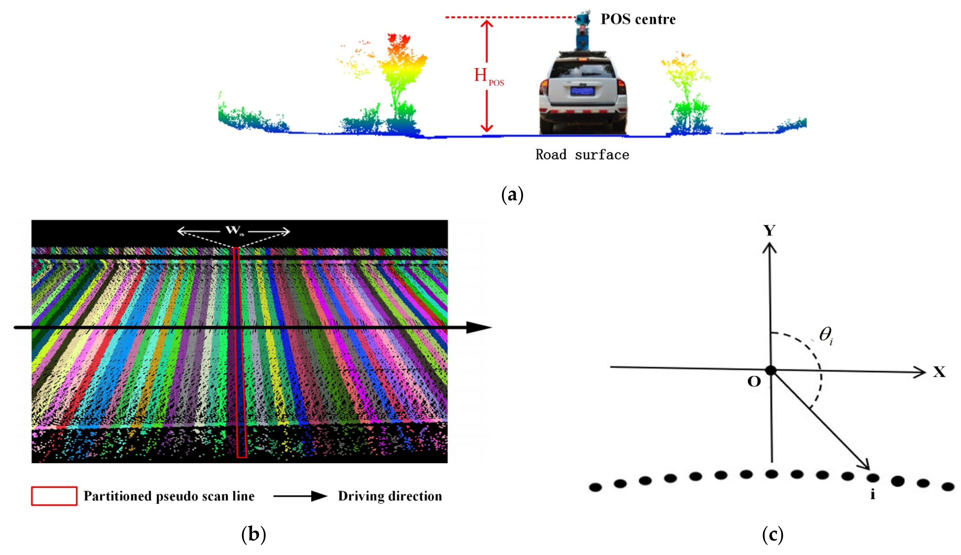
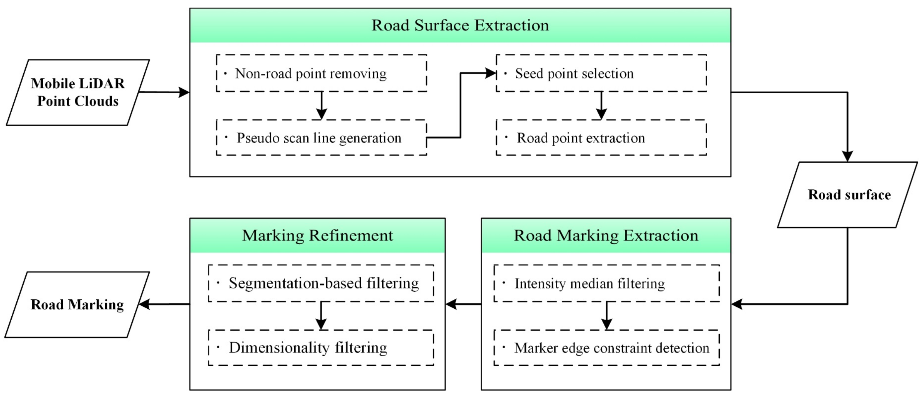
Establishing an efficient and reliable strategy to reduce the number of point clouds to be processed, including a pseudo-scan line-based organization data structure that could be used for road marking extraction from dense 3D point clouds.
(2)
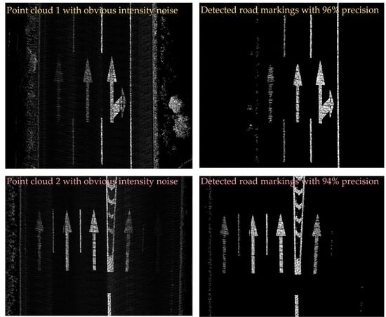
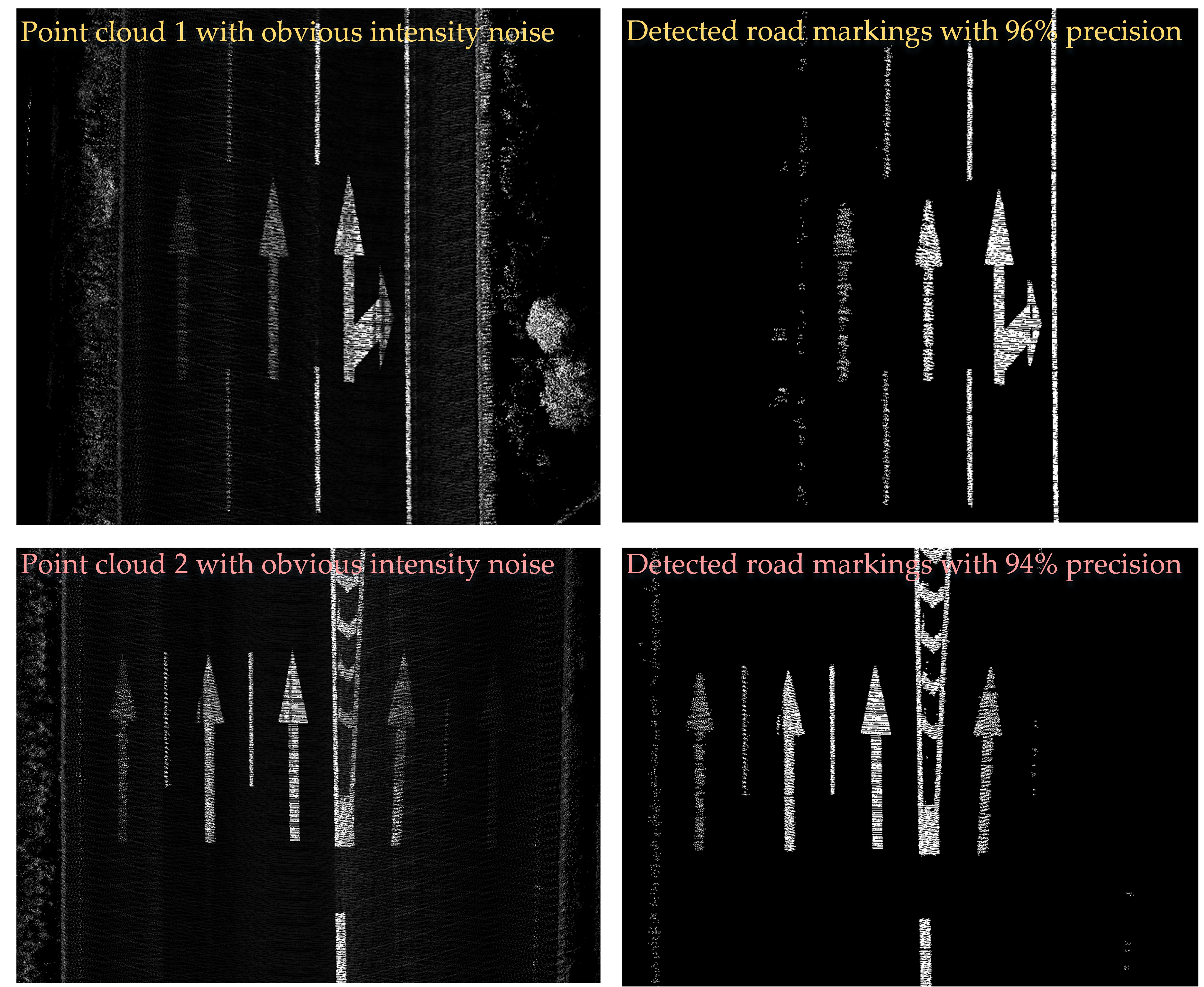
Presenting a density-based adaptive window median filter to suppress noise in different point-density and intensity-noise levels of MLS point clouds as well as a marker edge constraint detection (MECD) method for road marking edge extraction.
The paper is structured as follows. The next section describes the related processes of the proposed method. Section 3 analyzes extraction results of a quantitative evaluation and a comparative study. In Section 4, a discussion is presented for describing the applicability of the proposed detecting method. Conclusions are presented in Section 5.

2. Method

The proposed method was divided into three steps: (1) Road surface extraction, (2) road marking extraction, (3) road marking refinement. First, a nonroad point filter was applied to remove most nonroad points and then the remaining points were partitioned into different pseudo-scan lines. The road surface was precisely extracted using an extended moving fitting window filter. Road markings were extracted directly using the marker edge constraint detection (MECD) method after density-based adaptive window median filtering of intensity information. Finally, nonmarking points were eliminated by a segmentation-based filter and a dimensionality filter. An overview of the proposed method is illustrated in Figure 1.

2.1. Road Surface Extraction

It is time consuming and difficult to extract the road surface and road markings from a bulk of unstructured 3D points. As shown in Figure 2, the road surface was located under the POS (positioning and orientation system) centres and the POS height, H POS , which is the distance from a POS centre to the road surface, remained almost unchanged during data acquisition. To reduce the number of points, a nonroad point filter was applied based on the height difference, Δ h , between the trajectory and each point. A point was removed if its Δ h fell in the range from H POS   -   H th to H POS   +   H th . The predefined threshold H th is usually set to 0.5 m.
To simplify the data structure of point clouds and improve computational efficiency, the remaining points were partitioned into a set of consecutive pseudo-scan lines by a width threshold, W th , perpendicular to the driving direction, as shown in Figure 2a. Meanwhile, each pseudo-scan line was transformed into its corresponding local coordinate system. As shown in Figure 2b, the local coordinate system was constructed as the right-handed system, and the points inside the local coordinate system were arranged in decreasing order of their polar angles θ i . In the subsequent processing, road points and road marking points will be extracted, scan line by scan line, in the local coordinate systems. W th is usually set depending on the average distance interval between adjacent scan lines, such as from 0.05 m to 0.1 m in our experiments.
In most road scenes, road surfaces are classified as two typical types. As shown in Figure 3a, road surfaces I are directly bordered by curbs. As shown in Figure 3b, road surfaces II are not bordered by curbs but are separated by drainage channels. In a pseudo-scan line, there is an elevation jump between the road boundary and the curb of road surfaces I. Since the drainage channels cannot be scanned completely, there is a horizontal distance jump or an elevation jump between the road boundary and the curb of road surfaces II. The curbs or drainage channels are regarded as boundaries that separate the road surfaces and pavements. Therefore, the road surface can be extracted by detecting the jump features.
To extract road surface points, we developed an extended moving fitting window filter, as shown Figure 3. In a pseudo-scan line, a point that is right underneath and closest to the trajectory should be selected as a seed point. A certain number of points (usually define 20 points) are put into a fitting window and then fitted as a straight line using a least-squares fitting algorithm. From the seed point to the outer edges of the pseudo-scan line, the window is designed to slide point by point to detect jump features. This filter will be applied to the other side of the pseudo-scan line either when two adjacent points are determined as nonroad points or a jump in distance is detected in the current side. Both criteria related to the jump features are defined as follows.
(1)
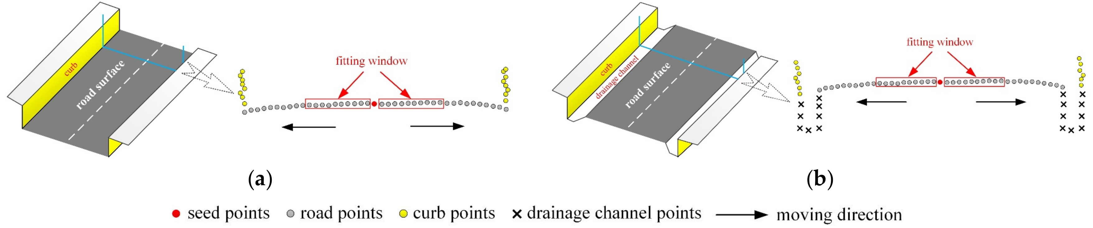
Elevation jump criterion. Since the elevations of road points in a local area are almost unchanged, a potential point is determined as a road point if the distance from the point to the fitted line is smaller than the threshold E th . E th represents the elevation difference between points at the road boundary and points at the curb, and is set here to 0.04 m.
(2)
Horizontal distance jump criterion. The distance from the current point to the outmost point in the window is calculated. The point is determined as a nonroad point if the distance is greater than the threshold D th . D th represents the width of the drainage channel and is set here to 0.7 m because the drainage channels are relatively narrow in the road environment of the datasets.

2.2. Road Marking Extraction

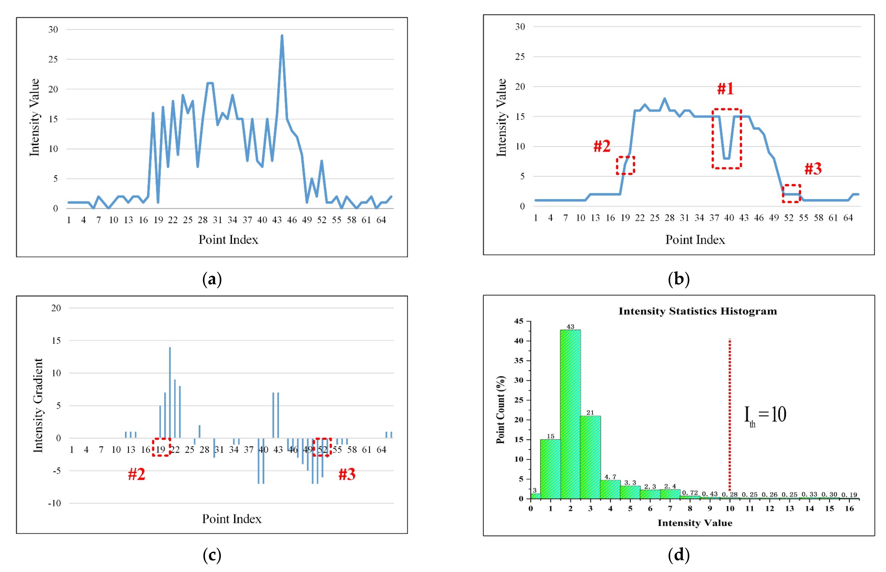
2.2.1. Intensity Median Filtering

Pulse energy is greatly affected by scanning distance [23,24]. Generally, the intensity values recorded by road marking points decrease with an increase in scanning distances. In the acquiring principle of multi-beam MLS systems, different beams collect point clouds at nonconsecutive scanning distances. As shown in Figure 4a, the intensity values of road marking points strongly fluctuate in a pseudo-scan line. The unstable intensity makes it difficult to accurately detect marking edges. Therefore, it is necessary to smooth the intensity values of road points.
The median filter is linear and uses the intensity median of points in the filtering window to replace the intensity value of one point at the window centre to suppress noise. Since the densities of points decrease away from the trajectory, the intensity values of points at marking edges may be smoothed in low-density regions. We applied a density-based adaptive window median filter to prevent over-smoothing. The size of the filtering window was changed adaptively according to different densities of points in a local region by Equation (1):
W s i z e = W max 2 ζ W max ζ W max , , , P n 0 , N 1 P n N 1 , N 2 P n N 2 , +
where W s i z e denotes the size of the filtering window. W max denotes the maximum size of filtering window and was set here to 7. P n denotes the number of points in a radius neighbourhood. N 1 and N 2 are two interval values of the number of points and were set to 10 and 15 in the experiments. ζ denotes the scale factor and was set to 2. As shown in Figure 4b, the intensity values of road marking points became smooth, whereas the intensity values of points at marking edges remained after smoothing.
.

2.2.2. Marker Edge Constraint Detection

Road markings often show higher reflected intensity values than nearby road points because they are made of white or yellow materials. In the past, some researchers used the intensity gradient to detect road marking edges from scan lines [18]. Even though the road surface has been smoothed, there are still some points that are not fully smoothed (see #1 in Figure 4) because of the complexity of multi-beam MLS data. They may be mistakenly detected as road marking edge points. To accurately detect road marking edges from pseudo-scan lines, we developed a marker edge constraint detector (MECD) method by combining the intensity gradient with the intensity statistics histogram. The intensity gradients of the points are estimated using Equation (2):
G i = I i I i k
where G i denotes the intensity gradient of i th point in a pseudo-scan line. I i k and I i denote the intensity values of the ( i k ) th and i th points, respectively. The k was empirically set to 3.
From the left-hand side to the right-hand side along a pseudo-scan line, the double edges of a road marking are defined as: The marking edge entering the road marking is called the left-hand edge and the marking edge leaving the road marking is called the right-hand edge. The left-hand edge point, such as point #2 in Figure 4, is a road marking point. Its intensity gradient is a positive value, and its intensity value is greater than the intensity values of its nearby nonmarking points. The right-hand edge point, such as point #3 in Figure 4, is a nonmarking point. Its intensity gradient is a negative value, and its intensity value is lower than the intensity values of the nearby road marking points. The MECD method is formulated as Equation (3):
P i Left - hand , i f G i > P th & I i > I th P i Right - hand , i f G i < N th & I i < I th
where P th and N th denote a positive gradient threshold and a negative gradient threshold. They are identified based on the intensity difference between marking edge points and surrounding road points. I th denotes an intensity threshold indicating the minimum intensity value of road marking points. In most road scenes, the proportion of road markings in the whole road surface is very small. To estimate the minimum intensity value, an intensity statistics histogram is counted based on the intensity information of the smoothed road surface. And a low-rate intensity value (i.e., value at the red vertical line in Figure 4) is chosen as I th .
To simplify double edges detection, the MECD method is normalized as the Equation (4).
f l a g = 1 1 0 , , , i f i f i f P i Left - hand P i Right - hand others
where the left-hand edge points, the right-hand edge points, and the other points are normalized into flag values with 1, −1, and 0, respectively. In pseudo-scan lines, each pair of left-hand edge points and right-hand edge points, respectively, correspond to a pair of flag vales with 1 and −1 after normalizing and the points between each pair of flag vales with 1 and −1 are extracted as road marking points.

2.3. Road Marking Refinement

To eliminate nonmarking points that do not connect to road markings, a segmentation-based filter was applied. All points were first grouped into individual segments using Euclidean distance clustering. A nonmarking segment can only be partitioned into a few pseudo-scan lines. If the line number of scan lines contained in a cluster is less than a predefined line number threshold M th , automatically estimated by Equation (5), the cluster is determined as noise and eliminated.
M th = I N T ( L min W th ) + 1
where L min represents the length of the shortest road marking in the datasets along the driving direction. W th is the width threshold of the pseudo-scan line generation mentioned in Section 2.1. In most road environments, the shortest road marking is the stop line with a length of 0.2 m, and thus L min is usually set to 0.2 m.
In a radius neighbourhood, the real marking points are structured into a 2D plane while the nonmarking points are structured into a 1D line. A dimensionality filter proposed by Lalonde et al. [25] is applied to eliminate the final remaining nonmarking points. A point is determined as noise and eliminated, if its linearity, according to the eigenvalues λ 1 , λ 2 , λ 3 of the covariance matrix, is greater than a linearity threshold L th . L th is usually set to 0.95.

3. Result

To test the performance of the proposed method, two datasets acquired by a multi-beam MLS system were employed in the experiments. The installed system consisted of a low-cost Velodyne VLP-16 laser scanner, an integrated navigation system (Global Positioning System/Inertial Measurement Unit, GPS/IMU), and a wheel-mounted distance measurement indicator (DMI). The datasets were scanned in a highway region. Dataset I presents a drainage channel at the right-hand side of road boundary, and it covers a road with length of 72 m, 1.7 million points, and a density of 762 points/m2. Dataset II absents obvious raised curbs at road surface boundary, and it covers a road with length of 46 m, 0.9 million points, and a density of 915 points/m2. As can be seen in Figure 5, the reflected laser pulse intensities of multi-beam MLS points were very inconsistent and the point clouds distributed unevenly on the road surface.

3.1. Parameter Sensitivity Analysis

The positive gradient threshold P th , negative gradient threshold N th , and intensity threshold I th in the MECD method are three key parameters whose thresholds with different values will affect the performance of the proposed method. The multi-beam MLS data (i.e., dataset II) were firstly tested using a set of parameter configurations to demonstrate the relations between road marking extraction and the thresholds.
P th describes the sensitivity of detecting the left-hand edge using the MECD method. The road markings extracted using P th with different values are illustrated in Figure 6a–c. It can be observed that the bigger P th was, the fewer nonmarking points were extracted (see #1 and #2 in Figure 6), but a few road marking points (see #3 in Figure 6) were missed when P th = 6. To validate the sensitivity of N th used to detect the right-hand edge, we tested the performance of the MECD method with different values of N th , as shown in Figure 6d–f. It is shown from #4 to #6 in Figure 6 that the right-hand edge points were gradually correctly detected when N th was increased from −6 to −2. I t h with different values was selected from the intensity statistics histogram to validate the sensitivity of road marking extraction. The test results are shown in Figure 6g–i. It can be seen that fewer nonmarking points (see #7 and #8 in Figure 6) were mistakenly extracted with a bigger I t h , but many road marking points (see #9 in Figure 6) were missed.
The higher the thresholds were set, the higher the precision of the MECD method. This is because the method can correctly identify road marking points with high-intensity values as marking edge points. However, a few road marking points, especially low-intensity marking points at marking edges, may be ignored if they were set too large. To completely extract road markings and suppress noise, the algorithm parameters of the MECD method used in the experiments were set to P th = 2, N th = −2, and I t h = 10.

3.2. Experiments

In pseudo-scan line-based local coordinate systems, the moving fitting window filter was applied to extract road points. The road surfaces extracted from the two datasets are illustrated in Figure 7a,b. The yellow points are road points, and the white points are nonroad points. The filter is reliable and can extract the road surfaces completely. Note that there are four segments (see #1, #2, #3, and #4 in Figure 7) in the outer edges of multi-beam MLS data. The points inside the segments were directly removed after seed point selection because seed points and road marking points were absent.
The MECD method extracts road marking points by detecting each pair of double edges from pseudo-scan lines. Road markings extracted from the two datasets are shown in Figure 7c,d, where various types of road markings, including arrows, rectangles, and hatch road markings, were successfully extracted. As can be seen, the method was able to extract road markings completely correctly from multi-beam MLS data, which proved its effectiveness and robustness for road marking extraction. However, we found a few failures in which some road marking points, especially road markings at the right-hand side of road surface (see #5 in Figure 7), were missed. This is because the laser pulse energy decreases with an increase in scanning distance. Those road markings were far away from the laser scanner and, thus, their intensity values were very low and were almost equal to those of nearby road points. A lot of nonmarking points (see #6 in Figure 7) were mistakenly extracted from the road boundary of dataset II because the boundary was covered with a bulk of weeds.
The segmentation-based filter and dimensionality filter were applied to eliminate nonmarking points in the extracted road markings. The filters eliminated the nonmarking points by identifying the spatial characteristics of the nonmarking segments. The refinement results are illustrated in Figure 7e,f. Almost all of the nonroad marking points were eliminated from the extracted road markings. The results indicate that the proposed method is effective for road marking refinement. However, a part of the noises, such as nonroad marking points in #7 in Figure 7, were not eliminated. This is because the nonroad marking points were distributed sparsely and showed irregular spatial characteristics and, thus, it was hard to eliminate them sufficiently.

3.3. Comparative Study

Our method was compared with an existing method proposed by Yu [16]. The two methods both directly extract road markings from mobile LiDAR point clouds in contrast to feature image-based methods, which ensures fairness of comparison. For Yu’s method, the road surface was divided into a set of segments, and then the road marking points were extracted from each segment using Otsu’s threshold algorithm and noise was removed using a spatial density filter. The road markings extracted by Yu’s method from the road surface of the two datasets are shown in Figure 8.
As seen from the results of the comparative study in Figure 7e,f and Figure 8, Yu’s method missed a bulk of road marking points (see #1 in Figure 8), especially road marking points with low-intensity values at marking edges. This is because these marking points’ intensity values were lower than the Otsu thresholds in their corresponding segments. In addition, there were more nonmarking points in the exit lane (see #2 in Figure 8) in the results extracted by Yu’s method. This is because the reflected laser pulse intensities also depended on material abrasion. The vehicles were only allowed to drive in the exit lane at low speed. The exit lane was less worn and, thus, the intensity values of the road points were relatively higher. The results extracted by our method only had a few nonmarking points in the same areas.
To quantitatively evaluate the performance of the two methods, reference datasets (truth) of the road marking points were manually labeled by visual inspection of the two datasets. The recall, precision, and Matthews correlation coefficient (MCC) index described in Equation (6) were employed [26].
r e c a l l = T P T P + F N p r e c i s i o n = T P T P + F P M C C = T P × T N F P × F N ( T P + F P ) ( T P + F N ) ( T N + F P ) ( T N + F N )
where T P , F N , and F P represent the number of correctly extracted, undetected, and falsely extracted road marking points, and T N represents the number of correctly detected nonmarking points.
The results of the quantitative evaluations are listed in Table 1 and Table 2. It can be seen that our method demonstrates better performance for road marking extraction from multi-beam MLS points. Our method achieves about 90% average recall and about 95% average precision, whereas Yu’s method achieves about 75% average recall and about 82% average precision. This is because the reflected laser pulse intensities of multi-beam MLS points are very inconsistent, and Yu’s method is difficult to identify marking points with low-intensity values in road markings. Our method’s average MCC was about 15% higher than that of Yu’s method.
The two methods were implemented in C++ programming language. The processing without parallel computing was performed on an ordinary personal laptop with an Intel Core i7-10510U CPU with 8 GB RAM. The running time of each processing stage in seconds is listed in Table 3. For the two datasets, about 40% of the total time was spent in road marking extraction because intensity median filtering was time consuming. The k-d tree costed a lot of memory to structure the radius neighbourhoods of each point. Our method was about 3 s on the average total and was slightly a bit time consuming. However, this can be improved by parallel computation scan line by scan line.

4. Discussion

Previous methods were mainly designed for road marking detection from mono-beam MLS points, while the proposed method aimed to accurately detect road markings from multi-beam MLS points. Additionally, our method, unlike most of the methods reported in the literature [9,12,27,28,29], does not depend on converting 3D point clouds into 2D images; therefore, the loss of accuracy was avoided effectively.
The points were partitioned into pseudo-scan lines perpendicularly to the driving direction. Therefore, our method successfully solved the problem that the number of point clouds to be processed is significantly reduced and multi-beam MLS points cannot be organized into the scan line structure using time stamps [30] and angle field [18]. This structure is also suitable for parallel and real-time/online processing. Of course, the correct size of pseudo-scan lines should be determined for different MLS data with different densities. Enough points can be organized into each pseudo-scan line using a larger width threshold, but the computation efficiency may decline. When using a width threshold that is too small, the road surface may not be completely extracted.
The moving fitting window filter precisely extracted the road surface by detecting jump features between the road boundaries and the curbs. The filter can be applied not only to road surface with the curbs but also to some road surface without curbs. All points inside a pseudo-scan line will be regarded as road points and extracted if jump features were not detected in the pseudo-scan line. Road surface extraction may be affected by vehicles on the road surface because the elevation jump between the vehicle and road surface may be mistakenly detected as the road boundary. To decrease the influence of vehicles, data acquisition should avoid rush hours.
Our method worked effectively for road marking extraction from noisy multi-beam MLS points, which is beneficial to MLS technology that is widely used in road information collection and promotes the development of unmanned driving. However, the MECD method may be less accurate for extracting badly worn road markings and emergency lanes, because I th selected from the intensity statistics histogram is a globally optimal threshold. The limitation of the globally optimal threshold makes it difficult to separate road marking points with similar intensities to road points from local road surface.

5. Conclusions

Most of the existing methods extract road markings from point clouds acquired by high-precision mono-beam MLS systems. However, mono-beam MLS systems are expensive. The high cost limits MLS technology from being applied to road information collection on a large scale. In this paper, we presented an accurate method to directly extract road markings from low-cost, multi-beam system scanning data. The proposed method applied a nonroad point filter to eliminate most nonroad points, and then the remaining points were partitioned into different pseudo-scan lines and transformed into corresponding pseudo-scan line-based local coordinate systems. An extended moving fitting window filter was applied to extract the road surface and further reduce the number of points. A density-based adaptive window median filter was applied to smooth the intensity information of the road surface. The MECD method was applied to extract the road markings through detecting each pair of left-hand edge point and right-hand edge point from each pseudo-scan line. The extracted road markings were refined by a segmentation-based filter and a dimensionality filter to eliminate nonmarking points. The quantitative evaluation showed that the proposed method achieved average recall, precision, and MCC of 90%, 95%, and 92%, respectively, for road marking detection from multi-beam scanning point clouds. The extracted road markings can be modeled to make high-precision maps. The road markings on high-precision maps are not only used by traffic management departments to direct traffic activities but also provide detailed instructions for the navigation of self-driving vehicles. Future work will focus on the combined application of our method with deep-learning methods for road marking classification and real-time environmental detection.

Author Contributions

onceptualization, Junxiang Tan; data curation, Ronghao Yang and Xinyu Chen; funding acquisition, Junxiang Tan; investigation, Shaoda Li; methodology, Ronghao Yang and Qitao Li; software, Qitao Li and Junxiang Tan; supervision, Shaoda Li; validation, Ronghao Yang, Shaoda Li, and Xinyu Chen; visualization, Xinyu Chen; writing—original draft, Ronghao Yang, Qitao Li, and Junxiang Tan; writing—review and editing, Qitao Li and Xinyu Chen. All authors have read and agreed to the published version of the manuscript.

Funding

This research was funded by the Startup Foundation of Chengdu University of Technology, grant number 10912-2019KYQD0727, and also funded by the National Natural Science Foundation of China, grant number 41771444.

Acknowledgments

The authors gratefully thank the editor and anonymous reviewers for their constructive comments.

Conflicts of Interest

The authors report no potential conflict of interest.

References

  1. Hoffmann, G.M.; Tomlin, C.J.; Montemerlo, M.; Thrun, S. Autonomous automobile trajectory tracking for off-road driving: Controller design, experimental validation and racing. In Proceedings of the American Control Conference, New York, NY, USA, 9–13 July 2007. [Google Scholar]
  2. Holgado-Barco, A.; Riveiro, B.; González-Aguilera, D.; Arias, P. Automatic inventory of road cross-sections from mobile laser scanning system. Comput. Aided Civ. Infrastruct. Eng. 2017, 32, 3–17. [Google Scholar] [CrossRef] [Green Version]
  3. Li, Z.; Tan, J.; Liu, H. Rigorous boresight self-calibration of mobile and UAV LiDAR scanning systems by strip adjustment. Remote Sens. 2019, 11, 442. [Google Scholar] [CrossRef] [Green Version]
  4. Mandlburger, G.; Pfennigbauer, M.; Wieser, M.; Riegl, U.; Pfeifer, N. Evaluation of a novel UAV-bornet opo-bathymetric laser profiler. ISPRS Int. Arch. Photogramm. Remote Sens. Spat. Inf. Sci. 2016, 41, 933–939. [Google Scholar] [CrossRef]
  5. Yan, L.; Tan, J.; Liu, H.; Xie, H.; Chen, C. Automatic non-rigid registration of multi-strip point clouds from mobile laser scanning systems. Int. J. Remote Sens. 2018, 39, 1713–1728. [Google Scholar] [CrossRef]
  6. Glennie, C.L.; Kusari, A.; Facchin, A. Calibration and stability analysis of the VLP-16 laser scanner. ISPRS Int. Arch. Photogramm. Remote Sens. Spat. Inf. Sci. 2016, 9, 55–60. [Google Scholar] [CrossRef]
  7. Pierzchała, M.; Giguère, P.; Astrup, R. Mapping forests using an unmanned ground vehicle with 3D LiDAR and graph-SLAM. Comput. Electron. iAgric. 2018, 145, 217–225. [Google Scholar] [CrossRef]
  8. Miadlicki, K.; Pajor, M.; Sakow, M. Real-time ground filtration method for a loader crane environment monitoring system using sparse LIDAR data. In Proceedings of the 2017 IEEE International Conference on INnovations in Intelligent SysTems and Applications (INISTA), Gdynia, Poland, 3–5 July 2017. [Google Scholar]
  9. Yang, B.; Fang, L.; Li, Q.; Li, J. Automated extraction of road markings from mobile LiDAR point clouds. Photogramm. Eng. Remote Sens. 2012, 78, 331–338. [Google Scholar] [CrossRef]
  10. Guan, H.; Li, J.; Yu, Y.; Ji, Z.; Wang, C. Using mobile LiDAR data for rapidly updating road markings. IEEE Trans. Intell. Transp. Syst. 2015, 16, 2457–2466. [Google Scholar] [CrossRef]
  11. Kumar, P.; McElhinney, C.P.; Lewis, P.; McCarthy, T. Automated road markings extraction from mobile laser scanning data. Int. J. Appl. Earth Obs. Geoinf. 2014, 32, 125–137. [Google Scholar] [CrossRef] [Green Version]
  12. Jung, J.; Che, E.; Olsen, M.J.; Parrish, C. Efficient and robust lane marking extraction from mobile lidar point clouds. ISPRS J. Photogramm. Remote Sens. 2019, 147, 1–18. [Google Scholar] [CrossRef]
  13. Li, L.; Zhang, D.; Ying, S.; Li, Y. Recognition and reconstruction of zebra crossings on roads from mobile laser scanning data. ISPRS Int. J. Geo Inf. 2016, 5, 125. [Google Scholar] [CrossRef]
  14. Ma, L.; Li, Y.; Li, J.; Wang, C.; Wang, R.; Chapman, M. Mobile laser scanned point-clouds for road object detection and extraction: A Review. Remote Sens. 2018, 10, 1531. [Google Scholar] [CrossRef] [Green Version]
  15. Yang, B.; Liu, Y.; Dong, Z.; Liang, F.; Li, B.; Peng, X. 3D local feature BKD to extract road information from mobile laser scanning point clouds. ISPRS J. Photogramm. Remote Sens. 2017, 130, 329–343. [Google Scholar] [CrossRef]
  16. Yu, Y.; Li, J.; Guan, H.; Jia, F.; Cheng, W. Learning hierarchical features for automated extraction of road markings from 3-D mobile LiDAR point clouds. IEEE J. Sel. Top. Appl. Earth Obs. Remote Sens. 2015, 8, 709–726. [Google Scholar] [CrossRef]
  17. Wang, J.; Zhao, H.; Wang, D.; Chen, Y.; Zhang, Z.; Liu, H. GPS trajectory-based segmentation and multi-filter-based extraction of expressway curbs and markings from mobile laser scanning data. Eur. J. Remote Sens. 2018, 51, 1022–1035. [Google Scholar] [CrossRef]
  18. Yan, L.; Liu, H.; Tan, J.; Li, Z.; Xie, H.; Chen, C. Scan line based road marking extraction from mobile LiDAR point clouds. Sensors 2016, 16, 903. [Google Scholar] [CrossRef] [PubMed]
  19. Soilan, M.; Riveiro, B.; Martinez-Sanchez, J.; Arias, P. Segmentation and classification of road markings using MLS data. ISPRS J. Photogramm. Remote Sens. 2017, 123, 94–103. [Google Scholar] [CrossRef]
  20. Wen, C.; Sun, X.; Li, J.; Wang, C.; Guo, Y.; Habib, A. A deep learning framework for road marking extraction, classification and completion from mobile laser scanning point clouds. ISPRS J. Photogramm. Remote Sens. 2019, 147, 178–192. [Google Scholar] [CrossRef]
  21. Chen, S.; Zhang, Z.; Zhong, R.; Zhang, L.; Ma, H.; Liu, L. A dense feature pyramid network-based deep learning model for road marking instance segmentation using MLS point clouds. IEEE Trans. Geoence Remote Sens. 2020, 1–17. [Google Scholar] [CrossRef]
  22. Cheng, Y.-T.; Patel, A.; Wen, C.; Bullock, D.; Habib, A. Intensity thresholding and deep learning based lane marking extraction and lane width estimation from mobile light detection and ranging (LiDAR) point clouds. Remote Sens. 2020, 12, 1379. [Google Scholar] [CrossRef]
  23. Tan, K.; Cheng, X. Intensity data correction based on incidence angle and distance for terrestrial laser scanner. J. Appl. Remote Sens. 2015, 9, 094094. [Google Scholar] [CrossRef]
  24. Alireza, K.; Michael, O.; Christopher, P.; Nicholas, W. A review of LiDAR radiometric processing: From ad hoc intensity correction to rigorous radiometric calibration. Sensors 2015, 15, 28099–28128. [Google Scholar] [CrossRef] [Green Version]
  25. Lalonde, J.-F.; Vandapel, N.; Huber, D.F.; Hebert, M. Natural terrain classification using three-dimensional ladar data for ground robot mobility. J. Field Robot. 2006, 23, 839–861. [Google Scholar] [CrossRef]
  26. Yan, L.; Li, Z.; Liu, H.; Tan, J.; Zhao, S.; Chen, C. Detection and classification of pole-like road objects from mobile LiDAR data in motorway environment. Opt. Laser Technol. 2017, 97, 272–283. [Google Scholar] [CrossRef]
  27. Pankaj, K.; Paul, L.; Tim, M.C. The potential of active contour models in extracting road edges from mobile laser scanning data. Infrastructures 2017, 2, 9. [Google Scholar] [CrossRef]
  28. Yang, B.; Dong, Z.; Liu, Y.; Liang, F.; Wang, Y. Computing multiple aggregation levels and contextual features for road facilities recognition using mobile laser scanning data. ISPRS J. Photogramm. Remote Sens. 2017, 126, 180–194. [Google Scholar] [CrossRef]
  29. Arias, P.; Gonzalez-Jorge, H.; Riveiro, B.; Diaz-Vilarino, L.; Martinez-Sanchez, J. Automatic detection of zebra crossings from mobile LiDAR data. Opt. Laser Technol. 2015, 70, 63–70. [Google Scholar] [CrossRef]
  30. Yang, B.; Fang, L.; Li, J. Semi-automated extraction and delineation of 3D roads of street scene from mobile laser scanning point clouds. ISPRS J. Photogramm. Remote Sens. 2013, 79, 80–93. [Google Scholar] [CrossRef]
Figure 1. An overview of the proposed detection method.
Ijgi 09 00608 g001
Figure 2. Pre-processing for road surface extraction: (a) The POS (positioning and orientation system) height, H POS , from the POS centre to the road surface; (b) pseudo-scan lines rendered by random colours; (c) local coordinate system of points inside a pseudo-scan line.
Ijgi 09 00608 g002
Figure 3. Two typical types of road surfaces: (a) Road surfaces I; (b) road surfaces II. The crosses are drainage channel points that have not been scanned.
Ijgi 09 00608 g003
Figure 4. Intensity information of road markings: (a) Intensity values of a road marking in a pseudo-scan line before smoothing; (b) intensity values of a road marking in a pseudo-scan line after smoothing using a density-based adaptive window median filter; (c) intensity gradients of a road marking in a pseudo-scan line; (d) intensity statistics histogram of the smoothed road surface. Point #1 is the point that is not fully smoothed, point #2 is the left-hand edge point, and point #3 is the right-hand edge point. The intensity value at the red vertical line was chosen as the intensity threshold I th .
Ijgi 09 00608 g004
Figure 5. Overviews of the two datasets: (a) Dataset I rendered by the intensity attribute; (b) a detailed view of dataset I; (c) dataset II rendered by the intensity attribute; (d) a detailed view of dataset II.
Ijgi 09 00608 g005
Figure 6. Road markings extracted by the marker edge constraint detector (MECD) method with different thresholds: (a) P th = 2; (b) P th = 4; (c) P th = 6; (d) N th = −6; (e) N th = −4; (f) N th = −2; (g) I th = 8; (h) I th = 10; (i) I th = 12. P th , N th , and I th denote the positive gradient threshold, the negative gradient threshold, and the intensity threshold.
Ijgi 09 00608 g006
Figure 7. Extraction results of the two datasets: (a,b) Extracted road surfaces; (c,d) extracted road markings; (e,f) refined road markings.
Ijgi 09 00608 g007
Figure 8. Road markings extracted by Yu’s method [16]: (a) From dataset I; (b) from dataset II.
Ijgi 09 00608 g008
Table 1. Quantitative evaluation of road marking extraction using Yu’s method [16].
Yu’s MethodTruthTPFNFPTNRecall
(%)
Precision
(%)
MCC
(%)
Dataset I73,42954,57518,85421,9191,115,820747171
Dataset II40,89831,18097182530589,737769283
Average 758277
Table 2. Quantitative evaluation of road marking extraction using our method.
Our MethodTruthTPFNFPTNRecall
(%)
Precision
(%)
MCC
(%)
Dataset I73,42965,097833240791,605,861899491
Dataset II40,89836,75241461588883,497909692
Average 909592
Table 3. Running time for each step (unit: s).
DatasetsRoad Surface ExtractionRoad Marking ExtractionRoad Marking RefinementTotal Time
Dataset I1.51.71.24.4
Dataset II0.81.00.72.5
Average1.151.350.953.45
Publisher’s Note: MDPI stays neutral with regard to jurisdictional claims in published maps and institutional affiliations.

