Generation of Spatiotemporally Resolved Power Production Data of PV Systems in Germany


1
Department of Bioenergy, Helmholtz Centre for Environmental Research GmbH—UFZ, Permoserstraße 15, 04318 Leipzig, Germany
2
Bioenergy Systems Department, DBFZ Deutsches Biomasseforschungszentrum gGmbH, Torgauer Str. 116, 04347 Leipzig, Germany
*
Author to whom correspondence should be addressed.
ISPRS Int. J. Geo-Inf. 2020, 9(11), 621; https://0-doi-org.brum.beds.ac.uk/10.3390/ijgi9110621
Submission received: 31 July 2020
/
Revised: 20 October 2020
/
Accepted: 21 October 2020
/
Published: 24 October 2020
(This article belongs to the Collection Spatial and Temporal Modelling of Renewable Energy Systems)
Abstract
:Photovoltaics, as one of the most important renewable energies in Germany, have increased significantly in recent years and cover up to 50% of the German power provision on sunny days. To investigate the manifold effects of increasing renewables, spatiotemporally disaggregated data on the power generation from photovoltaic (PV) systems are often mandatory. Due to strict data protection regulations, such information is not freely available for Germany. To close this gap, numerical simulations using publicly accessible plant and weather data can be applied to determine the required spatiotemporal electricity generation. For this, the sunlight-to-power conversion is modeled with the help of the open-access web tool of the Photovoltaic Geographical Information System (PVGIS). The presented simulations are carried out for the year 2016 and consider nearly 1.612 million PV systems in Germany, which have been aggregated into municipal areas before performing the calculations. The resulting hourly resolved time series of the entire plant ensemble are converted into a time series with daily resolution and compared with measured feed-in data to validate the numerical simulations that show a high degree of agreement. Such power production data can be used to monitor and optimize renewable energy systems on different spatiotemporal scales.
1. Introduction
Photovoltaics in Germany have gone through turbulent times since they got off to a flying start with the introduction of the German Renewable Energy Act (EEG) in the year 2000. German companies quickly ascended to global leadership in solar cell technology before a collapse of the national panel production due to price pressure from global markets forced many of them to abandon their business in the following years. However, far from being among the countries with the most sunshine hours, Germany has one of the highest rates of photovoltaic (PV) power generation worldwide. With an installed capacity of 49.02 GW in 2019 starting from 0.11 GW in the year 2000 [1], the country ranked fourth in the world after leading the charge for several years, according to the International Renewable Energy Agency (IRENA) [2]. After abolition of the German 52 GW cap for solar incentives in June 2020, the PV capacity will continue to rise due to the decreasing levelized costs of electricity [3] and the required de-carbonization of the power sector to reach the national climate targets, e.g., cutting greenhouse gas emissions by at least 55% below 1990 levels by 2030, according to the Federal Climate Change Act (KSG 2019).
In contrast to conventional power plants focused on big and centralized producers, thousands of small and distributed solar panel operators have become an important part of the German electricity sector. The rapid advancement of photovoltaics in Germany during recent years not only has an essential impact on power grids but on many other fields of the power sector as well, triggering the need for further research. Thus far, current energy studies often contain power generation data of PV systems with a high spatial resolution, but lack a high temporal resolution, such as the analysis of the energy transition in the German power sector [4] or the high-resolution determination of the technical potential for roof-top systems in Germany [5]. To gain a better understanding of the challenges for a faster changing energy sector due to increasing variable renewables, spatiotemporal distributions of the electricity production, e.g., down to municipal and hourly resolutions, will become more important for future research. Especially, regional studies and decision makers can benefit from such data, e.g., to mitigate possible dark doldrums in the power supply on a local scale [6] or to promote the adoption of new PV systems depending on the geographical region [7].
However, the lack of such data for a required region and period, e.g., due to strict data protection regulations, makes it difficult for researchers and decision makers to find out the manifold effects of increasing renewable energies on regional power grids, the environment, and electricity markets. This study presents a model approach for creating highly resolved power production data of PV systems using publicly available plant and weather data, which can help to close the gap previously mentioned. Thus far, energy transition maps have been developed to support decision makers with data at a local level [4], but only on the basis of an annual electricity generation from PV systems. In order to be able to provide this information also for a shorter period of time, spatiotemporally resolved data are necessary, which are made available with the shown approach.
The remainder of this publication is organized as follows: Section 2 presents the used plant and weather data as well as the data needed for adaptation and validation of the numerical simulations. The PV model, which belongs to the physical models, and its implementation are described in Section 3. In Section 4, this simulation model is applied to a measured single PV system and also to an ensemble of 1.612 million PV systems sited in Germany. Subsequently, the resulting time series are aggregated and compared with measured feed-in data for the validation. Section 5 discusses the obtained results and introduces the first utilization examples using the presented simulations. Finally, this paper ends with brief conclusions in Section 6.
2. Data
This section presents the main data necessary for performing the numerical simulations including their origin and characteristics.
2.1. Plant Data
For the simulations, detailed plant data of the PV systems to be investigated are required. The used dataset originates from publicly available data of the four German transmission system operators (TSO), which are provided on their common internet platform (www.netztransparenz.de) [8]. After merging the four slightly different raw datasets, verifying the content with existing data studies [1,9], and filtering the TSO data by PV systems operated in the investigated year 2016, the final dataset consists of about 1.612 million plants. This dataset comprises all open-field and roof-top systems in Germany that receive guaranteed power feed-in prices, according to the EEG. The total installed capacity reaches 40.44 GW, which is in good agreement with the official value of 40.68 GW for 2016, according to the AGEE-Stat report [1]. The small deviation of less than 0.6% from the official sum indicates that almost all PV systems are included in the final dataset. For each PV system, the plant dataset contains the geographical location using the local administrative unit (LAU)-Id 1 or optionally the latitude and longitude coordinates, the installed capacity, and the date of (de-)commissioning, as shown in Table 1.
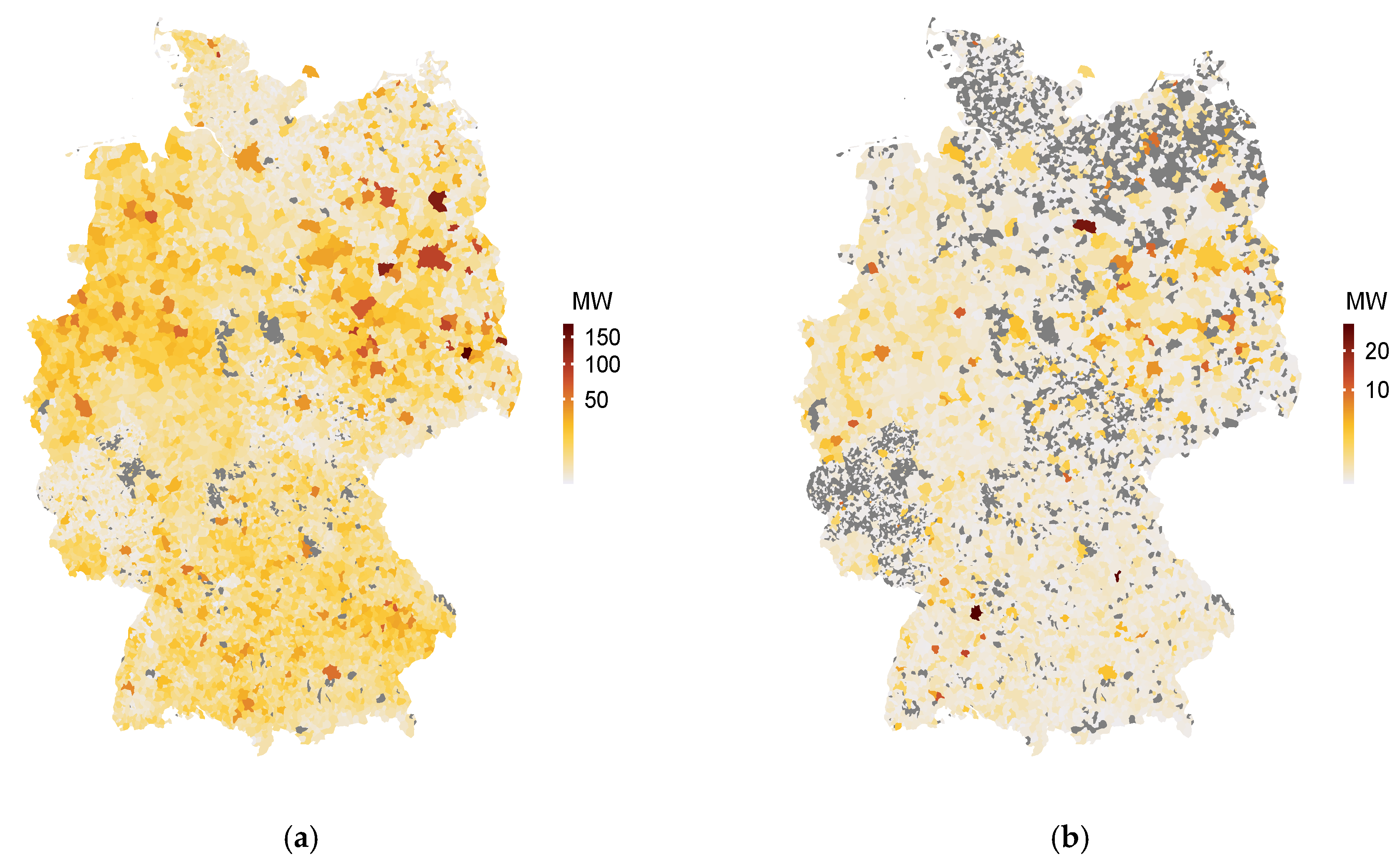
Due to the large number of individual plants and the lack of information about the exact position of roof-top systems, the PV systems are aggregated into municipal areas (LAU2), where they are located, before performing the numerical simulations. The corresponding installed capacity at the spatial resolution of LAU2 for 2016 and, as additional information, the intra-annual increase of the installed capacity for this year are depicted in Figure 1.
2.2. Input Parameters
For a reasonable adaptation of the simulation model, further input data are required, which are not included in the plant dataset shown in Table 1. Due to the lack of detailed technical information on each PV system, especially for roof-top systems, typical or averaged values have to be found for the unknown parameters. For example, the amount of the system loss and the existing module technology must be set for the calculation of the output power. The system loss describes all losses of a PV system, leading to the electricity actually delivered to the power grid being lower than the electricity generated by the PV modules. There are several reasons for this system loss, such as losses in cables, power inverters, and dirt or snow on the surface of the solar panels. Additionally, over the years the modules also tend to lose a bit of their performance and, therefore, the average output over the module lifetime is a few percent lower than the electrical output at the time of installation. For this system loss, the Photovoltaic Geographical Information System (PVGIS) recommends an overall value of 14% [10] that can result in too conservative estimations of the electrical output, as reported by the internet platform (www.photovoltaik-web.de) [11]. Such PV platforms often recommend values of about 10%, especially when PVGIS is used for a known PV system over a period without snow. Hence, for the simulation of the measured roof-top system in this study, a system loss of 10% is applied, which has been shown in the model adaptation to be a reasonable value. For the simulation of the plant ensemble over an annual period, additional losses have to be considered, e.g., possible feed-in interruptions and a power loss due to snow on the solar panels, and, therefore, a system loss of 14% is used for the entire ensemble. The technology of the PV modules is also not known for each PV system. Thus far, crystalline silicon is still the dominant semiconductor material for solar cell production worldwide [12]. Furthermore, in PVGIS, the consideration of module losses due to spectral variations of the sunlight and ambient temperature changes is currently only available for crystalline silicon and cadmium telluride panels [10]. Thus, crystalline silicon has been set as the module technology for the performed simulations. Moreover, for the needed inclination and azimuth angles of the solar panels, averaged values have to be found for the plant ensemble due to the lack of such information on each PV system.
2.3. Weather Data
High-resolution weather data are a key requirement for modeling the power generation from PV systems and, herein, the data quality plays an important role for the accuracy of the simulation results. For the area of Germany or Central Europe, different weather databases with various spatiotemporal resolutions are publicly accessible via the web interfaces of the meteorological services in Europe. So-called reanalysis data have emerged as a popular source of weather data for many power production studies. This type of weather data is calculated using numerical weather forecast models, re-running the models for a certain period in the past, and making corrections using existing meteorological measurements. In general, global reanalysis products have spatial resolutions that are not sufficient for the level of detail required in this study. Regional reanalysis data show typically higher spatial resolutions, e.g., the COSMO-REA6 weather product covering Europe with a spatial resolution of about 6 km [13], and, thus, would already enable detailed results with the presented PV model.
This study goes a step further and uses satellite-based weather data from the Satellite Application Facility on Climate Monitoring (CMSAF) collaboration [14] via the open-access web interface of PVGIS [10]. The CMSAF product in PVGIS has an hourly resolution and a spatial resolution of about 2.5 km for the area of Central Europe. Due to this high spatial resolution and the retrieval of the CMSAF data for each specified plant location in PVGIS, no additional interpolation of the weather data is necessary for the numerical simulations. Furthermore, the calculation of solar radiation at ground level from satellite images is achieved with comprehensive algorithms for the CMSAF weather data, which not only use satellite images but also atmospheric data on water vapor, aerosols, and ozone. Such algorithms generally work well but could fail in some cases. For instance, snow on the ground might be seen as clouds by the algorithms, which then calculate too low irradiances. Moreover, the necessary aerosol information used for the calculations consists of long-term average values over many years, therefore short-term changes in aerosols, e.g., due to volcanic eruptions or dust storms, are not well captured according to PVGIS [10]. Hence, solar radiation data obtained from satellite images have to be compared with measurements of ground-based stations to get an idea of the uncertainty of such satellite-based data. For the area of Central Europe, the accuracy of the CMSAF product is close to the confidence level of the ground-based measurements and significantly better than the target accuracy of 10 W/m² [15]. The high quality of these radiation data was also confirmed by recent validation studies [16]. In PVGIS, the hourly resolved time series for a certain period consists of the following information: date and time in coordinated universal time (UTC), output power, global irradiance on the inclined module plane, elevation angle of the sun in the sky, ambient temperature at 2 m, and total wind speed at 10 m above ground level. In order to obtain this information via the PVGIS web interface, the geographical position with latitude and longitude, installed capacity, inclination and azimuth angles of the PV modules, the required period of time, and, finally, the weather database must be specified. For the simulations shown in this paper, PVGIS 5.1 with the CMSAF weather product was used due to the high spatial resolution and accuracy.
2.4. Validation Data
The calculated results from numerical simulations should be compared with measurements on real systems in order to validate the underlying simulation model and assess its accuracy. However, an explicit validation of the sunlight-to-power conversion is not needed, because the calculation of the output power from PV modules is executed with the help of internal algorithms of PVGIS that have already been used and verified in various publications, e.g., [17,18]. Nevertheless, the presented model is validated with measured data of a single PV system to be sure that the applied input parameters lead to realistic simulation results. The used measurements, which are publicly available on the website of 100% Erneuerbare Energien (www.100pro-erneuerbare.com) [19], were carried out on a roof-top system sited in the town of Kronberg between 1 March and 31 July 2011.
Moreover, the PV model consists not only of physical algorithms for the sunlight-to-power conversion, but also considers intra-annual plant changes for the determination of the produced power, the transformation of the calculated time series into local time, and the appropriate spatiotemporal aggregation of the simulation results. Hence, the results from the numerical simulations showing the amount of the generated electricity should be validated with measured data. Feed-in time series of variable renewables like photovoltaics are only available for larger areas, such as entire countries. Thus, the simulation results from all plants are spatially aggregated to compare them with measured electricity data for the whole of Germany, provided by the internet platform SMARD of the Federal Network Agency (www.smard.de) [20]. From this platform, the measured total feed-in from all German PV systems was downloaded for the year 2016. It should be mentioned, that on three different days in 2016 no measurements were available by SMARD and, therefore, the resulting zero values are not considered for the validation and faded out in Figure 4.
3. Model
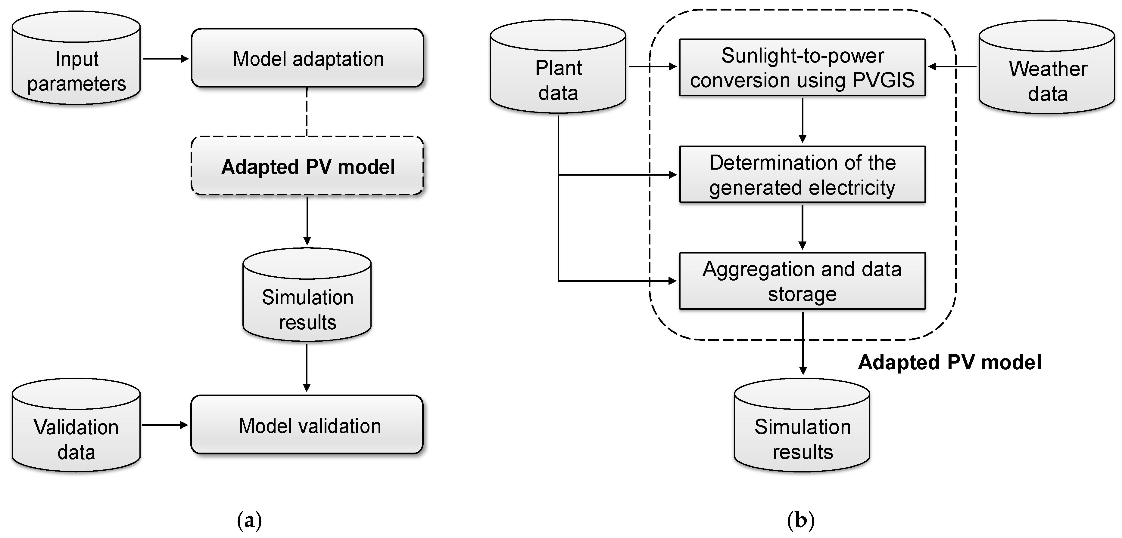
This section elaborates on the simulation model for the power production from PV systems in Germany. In general, the electricity generation for energy studies can be modeled either with statistical methods, e.g., auto-regressive and Monte Carlo models, or with physical models [21,22]. In contrast to statistical models [23], the results of physical models, such as the PV model presented herein, are based on high-resolution data from meteorological models or measurements. Hence, an advantage of physical compared to statistical models is the possibility to provide power production data on a highly resolved spatiotemporal scale. The flowcharts in Figure 2 outline the development process from adaptation to validation of the simulation model and its internal structure. The input and output data are symbolized as containers in both figures and the arrows indicate the direction of the data flow.
The plant and weather data as well as the required values for the known and unknown technical parameters represent the input data for the PV model, as shown in Figure 2. All specific data needed as input for the simulations are described in the first three subsections of Section 2. The required calculations, which are displayed as rectangles in Figure 2b, can be divided into the following main steps:
- Simulation of the output power from a PV system using PVGIS.
- Calculation of the generated electricity from this PV system.
- Aggregation of the simulation results and data storage.
The simulation of the output power from PV modules is performed with the help of internal algorithms of PVGIS. Therefore, the following effects are already covered for the sunlight-to-power conversion: Firstly, the calculation of the solar radiation on inclined planes. In general, satellite-based solar radiation data, as introduced in Section 2.3, deliver irradiances on the horizontal plane. However, most solar panels operate with an inclined surface to the horizontal plane. Thus, the satellite-retrieved data have to be converted into irradiances on the module surfaces, depending on the inclination and azimuth angles of the installed panels and the sun position in the sky. The algorithms of PVGIS use the satellite-based irradiances on the horizontal plane as input data to determine the corresponding values on tilted surfaces applying comprehensive calculations. Secondly, the consideration of shadows from the surrounding terrain. If the PV system is close to hills or mountains there may be times when the sun is behind them and the solar radiation will be reduced to that coming from blue sky or clouds. PVGIS uses information about the elevation of the terrain with a resolution of about 90 m, which means that for every 90 m there is a value for the ground elevation [10]. From these data, the height of the horizon around each PV system is calculated and, subsequently, the times when the sun is shadowed by hills or mountains. However, with a resolution of about 90 m, the concerning calculation model is not able to consider the effects of shadows from nearby objects, such as trees or houses. Thirdly and finally, in PVGIS, the effects of changes in the solar spectrum and the ambient temperature are taken into account for the determination of the output power in dependency of the module technology.
After calculating the output power from a PV system, the next step in the simulation model is to determine the generated electricity. For this, the value of the output power is multiplied by the given time slot, which is defined by the temporal resolution of the used weather product usually providing an hourly resolution. This step also takes into account the date of (de-)commissioning in order to consider possible intra-annual plant changes. Finally, the resulting time series is transformed from UTC to local time and sorted into its municipal area and, if necessary, converted into an additional time series with, e.g., daily resolution. After the described steps are performed for each PV system of the plant dataset, the time series of the whole ensemble are stored as comma-separated values for subsequent processing, e.g., using a geographical information system (GIS) or a web-based GIS application.
4. Results
This section presents the simulation results using the input data and the PV model previously described.
4.1. Simulation of a Single PV System
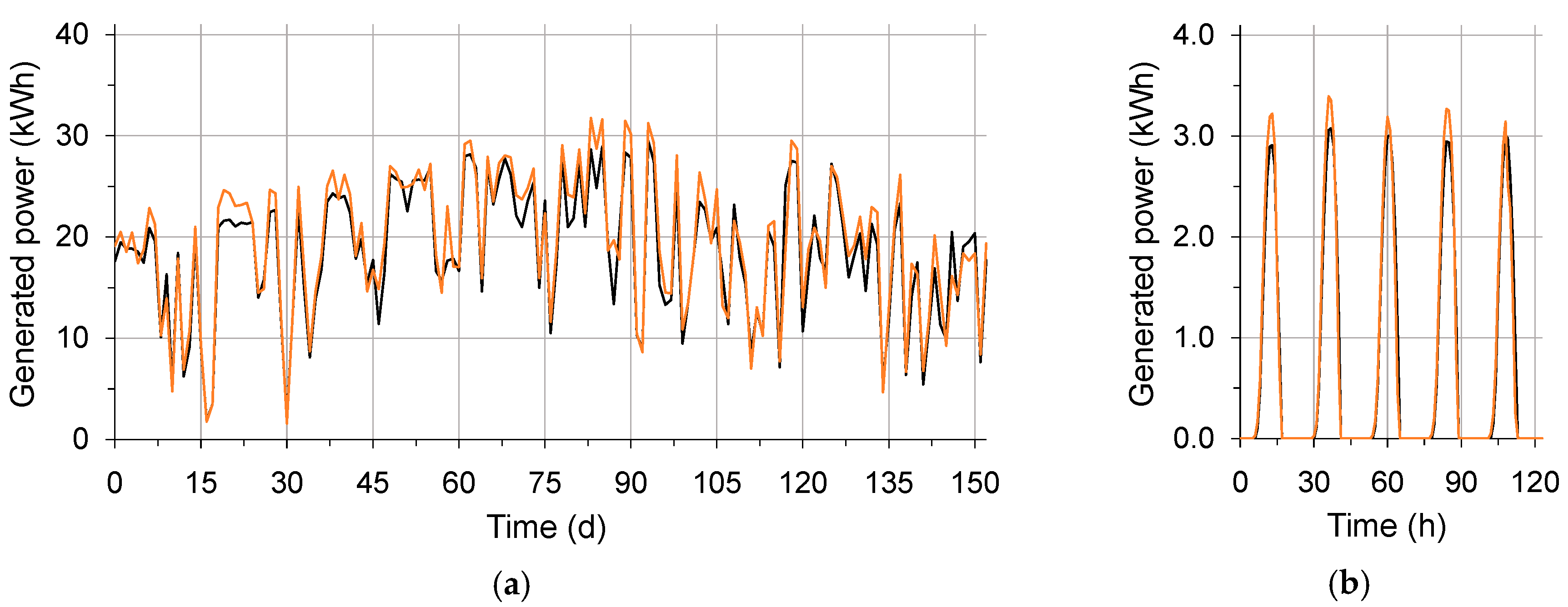
For proof of concept and model validation, the generated electricity from a single PV system is simulated and, afterwards, compared with measured data of this plant. The shown measurements were performed on a roof-top system located in Kronberg between 1 March and 31 July 2011, as introduced in Section 2.4. This PV system, with an installed capacity of 4.51 kW, has an azimuth angle of 40° to the west and an inclination of 30°, which are used for the simulations. Since no further information was available, typical values for the system loss and the module technology were applied to complete the model adaptation. As explained in Section 2.2, for the system loss, a value of 10% was used and the module technology was set to crystalline silicon. The simulated and measured time series, which were converted into daily resolutions for a better comparability, are shown in Figure 3a.
As depicted in Figure 3, the simulation model reproduces the pattern of the measured data very well (a) over the entire period and (b) also within the course of a day. Despite the existing deviations, the presented simulation model leads to realistic results with the chosen values for the unknown technical parameters. The root-mean-square error (RMSE) of the daily values, as a statistical measure for such deviations, is 1.9 kWh. In relation to the measured total electricity production of 2.98 MWh for this five-month period, the RMSE reaches a value of 0.06%. Hence, the adapted PV model and the CMSAF weather data can be used to simulate the electricity production for the whole plant ensemble.
4.2. Simulation of the Plant Ensemble
Given the lack of publicly available power generation time series of PV systems with a high spatiotemporal resolution, which was the main motivation for the simulation model presented herein, it is not possible to benchmark the performance of the entire plant ensemble on a spatial scale. However, if the simulated time series are spatially aggregated over Germany, they can be compared with publicly available feed-in measurements for all of Germany, provided by SMARD [20].
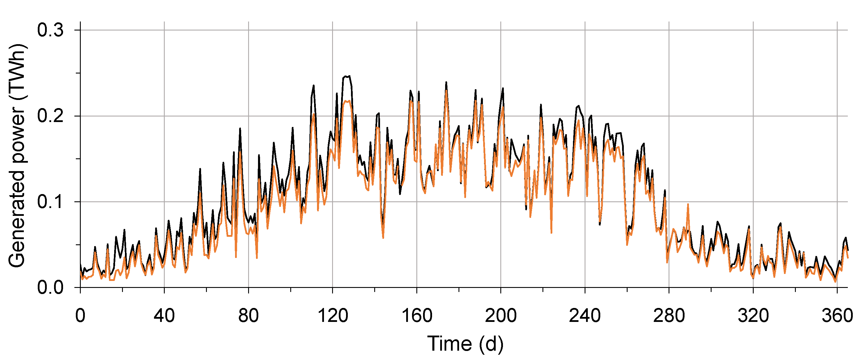
The PV model described in Section 3 was used to determine the electricity production from PV systems in Germany for 2016. Due to the large number of 1.612 million individual systems, the sites with PV systems were aggregated into municipal areas before the simulations were carried out. In this context, the geographical position of a municipal area was assigned by its center coordinates. Nevertheless, the peak power and the date of (de-)commissioning of the investigated year 2016 were considered individually for each PV system. Since no further information about the plant ensemble was accessible from official sources, a system loss of 14% was applied and the module technology was set to crystalline silicon for all plants, as described in Section 2.2. Moreover, for the needed inclination and azimuth angles of the solar panels, fixed values were used for the simulations. For the inclination, an angle of 20° was applied because open-field systems are often erected with slope angles in this range to minimize mutual shading of the solar panels, especially during the winter months when the sun is relatively low in the sky [24]. Furthermore, this value has been proven through many simulations to be also a reasonable average for the ensemble of existing roof-top systems. The azimuth angle was set to zero, which stands for a panel orientation in the southern direction. After performing the numerical simulations with these input parameters, the hourly resolved electricity generation time series were aggregated into a time series in order to compare the simulation results with the measured total feed-in from all PV systems in Germany. The simulated and measured time series, which were converted into daily resolutions for a better comparability, are depicted in the following diagram, as shown in Figure 4.
The simulated power generation, as depicted in Figure 4, is in good agreement with the measured feed-in pattern over the entire year. Additionally, it can be clearly seen that more electricity is typically produced during the summer months than in winter. The existing deviations are mainly caused by the following effects, which cannot be captured by the PV model:
- The uncertainties of the weather data and the fact of hourly averaged values.
- The use of typical values due to the lack of specific data for each PV system.
- Decrease of output power due to snow on the surface of the solar panels.
- Feed-in interruptions due to energy surpluses or module maintenance.
Nevertheless, with an RMSE of 13.9 GWh calculated for the daily values, the simulation results already show a good agreement with the measured feed-in data. In relation to the annual electricity production of 33.9 TWh, generated from all PV systems in Germany for the year 2016 according to SMARD, the RMSE reaches a value of 0.04%. The relatively high deviations between 15 and 23 January have been caused by snow on many PV modules in Germany, resulting in a higher simulated production than actually measured by SMARD. The deviations around the 125th day in 2016 with sunny weather, i.e., at the beginning of May, could have been caused by feed-in interruptions due to energy surpluses in the power grids, as there were many public holidays and vacation periods in Germany at that time and, therefore, less electricity was needed by industry.
5. Discussion
It could be clearly seen from the simulation results in Section 4 that, with the help of the presented PV model and the used publicly available data, sufficiently precise results can be achieved both for a single PV system and a large plant ensemble. Moreover, it could be also shown that with the use of typical or averaged values for the unknown technical parameters, the simulated power generation closely follows the measured feed-in pattern for Germany over the investigated year 2016. This year was chosen because the used weather data via PVGIS were only available until the end of 2016 at the writing of this paper. A further reason for this year was the continuation of the energy transition maps of 2015 [4] with electricity production data of PV systems in Germany for 2016. For these energy transition maps, a spatial resolution at LAU2 level is needed. Hence, the presented simulation model in combination with the CMSAF product in PVGIS, which provides a spatial resolution of 2.5 km [10], is useful for the generation of such maps. The publicly accessible web tool of renewables.ninja (www.renewables.ninja) [25,26], which also delivers the power production from PV systems for the required region and period, only employs global reanalysis (MERRA-2) weather data with a lower resolution of about 50 km [27], which are not sufficient for the level of detail needed for the energy transition maps of 2016. In contrast to PVGIS, renewables.ninja does also not consider shadows from the surrounding terrain for the calculation of the output power from PV modules.
For the performed simulations, nearly 1.612 million PV systems were taken into account and the obtained results reach a spatial resolution of municipal areas and have a temporal resolution of an hour. To the best of our knowledge, such a high spatiotemporal resolution of the electricity generation from PV systems in Germany considering almost all plants, which receive guaranteed power feed-in prices according to the EEG, has never been shown before.
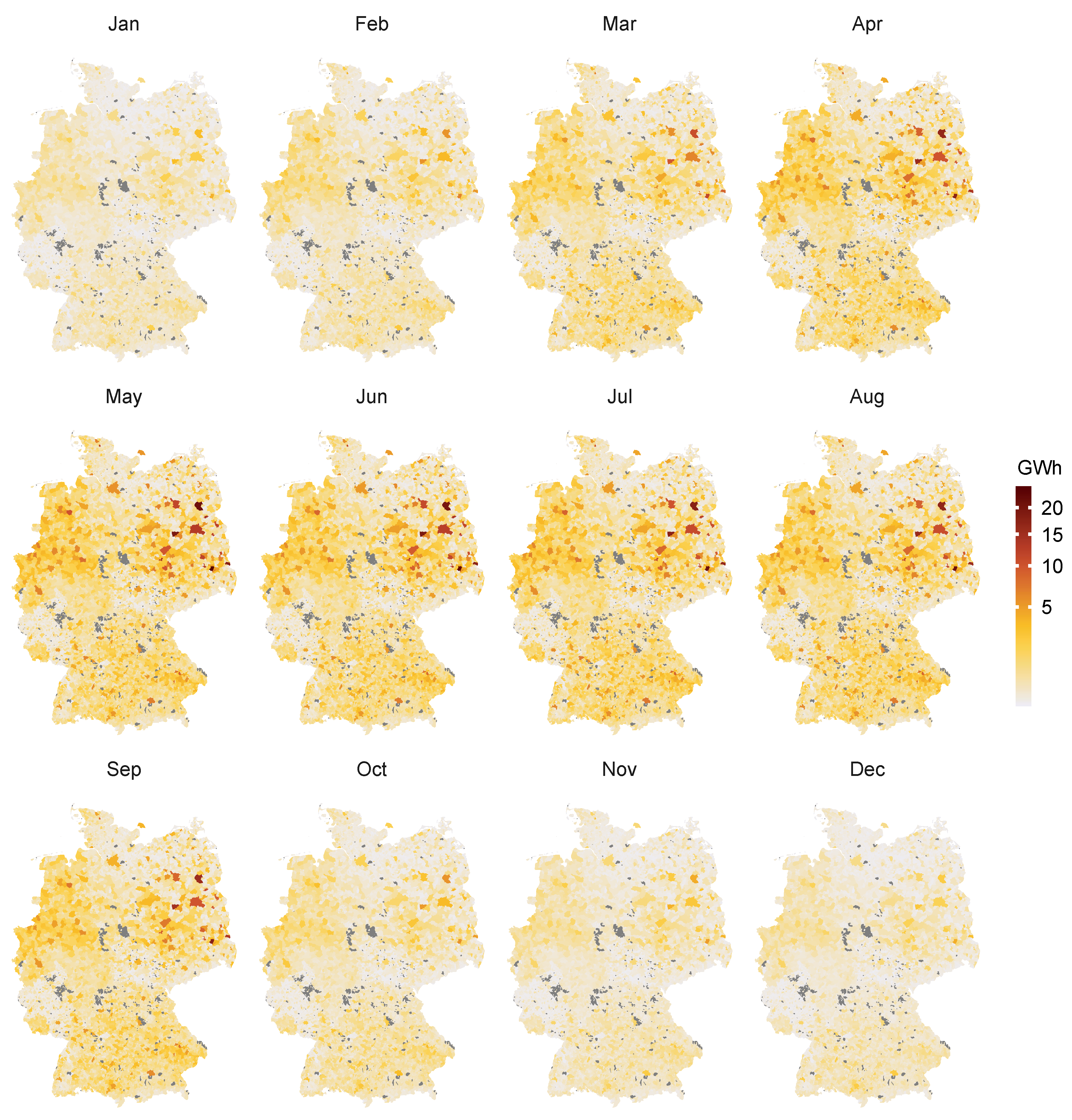
Understanding the power provision impact of existing PV systems on a highly resolved spatiotemporal scale is a prerequisite for successful integration of future variable renewables into regional power grids and associated electricity markets. As a first utilization example on this topic, Figure 5 shows the monthly power generation from PV systems at the spatial resolution of LAU2, based on the presented simulation results. In this way, regional advances of the energy transition towards higher shares of photovoltaics can be reliably monitored with the help of spatiotemporal distributions of the power production.
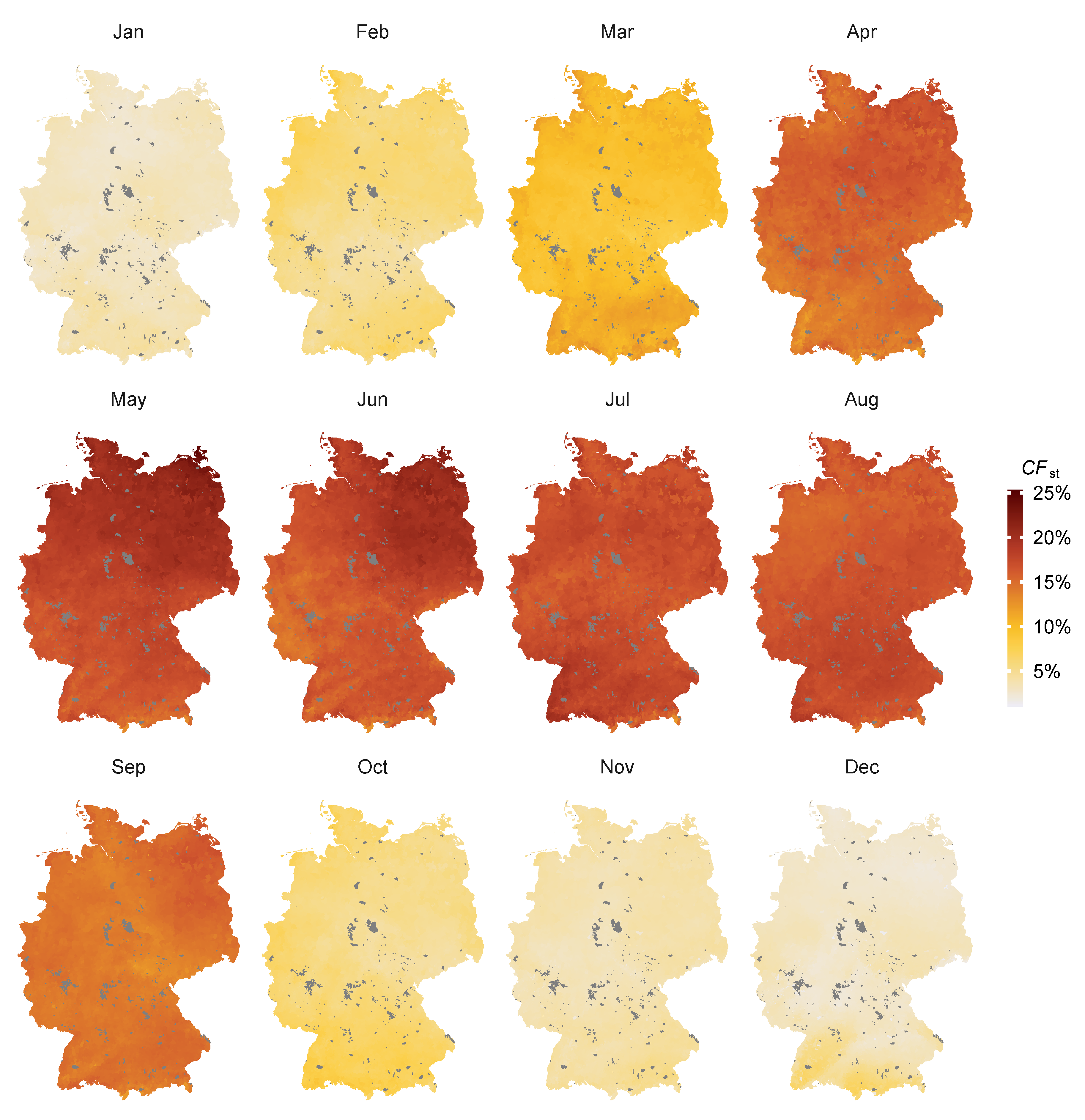
In addition, the simulation results can be used in combination with the installed capacity to calculate spatiotemporal capacity factors of PV systems to determine their efficiency depending on the considered region and period. For this, the spatiotemporal capacity factor CFst can be defined according to Equation (1):
In this equation, T stands for the considered period of time, Cpv is the PV capacity installed in the considered geographical area, and Epv is the generated electricity from PV systems in this region and period. Figure 6 shows the monthly capacity factors at the spatial resolution of LAU2 in Germany for 2016.
It can be clearly seen that the capacity factors of PV systems were much higher from April till September than during the winter months. In summer, i.e., from May till August, the spatiotemporal capacity factors reached maximum values of about 25%, with a peak of 25.3% on the island of Rügen in May. It is also noteworthy that the southern part of Germany had slightly higher capacity factors in December, while they were higher in the north-eastern part of Germany in June and September for the year 2016.
6. Conclusions
This study has presented new ideas for achieving highly resolved spatiotemporal electricity generation data of PV systems in Germany with the help of numerical simulations. It was an objective of this paper to create a simulation model, in which the focus was set on a very transparent, easy to imitate, and sufficiently precise model approach. To contribute to such an approach, the plant and weather data needed for the simulation model should be publicly accessible to give potential users the opportunity to develop their own simulations based on the presented ideas. It was clearly shown that the presented PV model can be an alternative to calculate highly resolved power generation data with the help of publicly available plant and weather data. Thus, based on the shown model structure and the open-access web tool of PVGIS, it is possible to create solid electricity production data from PV systems in Germany using open-source programming languages, such as Python or R.
Moreover, the shown PV model can be applied to other regions or countries without any changes, if the required plant and weather data are available for these areas. In addition, it can be also used with different weather products in PVGIS, which possess various resolutions and cover different regions around the world [10]. Such spatiotemporally resolved time series can also help to evaluate the electricity generation from PV systems for extreme weather events, e.g., long periods of heavy fog or snow. Many other applications, e.g., site assessment studies for future PV systems [28,29], can benefit from power production data delivered by the simulation model presented herein.
Author Contributions
Conceptualization, Reinhold Lehneis; Methodology, Reinhold Lehneis and David Manske; Software, David Manske and Reinhold Lehneis; Validation, Reinhold Lehneis; Formal Analysis, Reinhold Lehneis and David Manske; Investigation, Reinhold Lehneis and David Manske; Resources, David Manske and Reinhold Lehneis; Data Curation, David Manske; Writing—Original Draft Preparation, Reinhold Lehneis; Writing—Review and Editing, Reinhold Lehneis, David Manske, and Daniela Thrän; Visualization, David Manske and Reinhold Lehneis; Supervision, Daniela Thrän; Project Administration, Daniela Thrän. All authors have read and agreed to the published version of the manuscript.
Funding
This research received general funding from the Helmholtz Association of German Research Centres.
Conflicts of Interest
The authors declare no conflict of interest.
References
- BMWi Zeitreihen zur Entwicklung der erneuerbaren Energien in Deutschland unter Verwendung von Daten der Arbeitsgruppe Erneuerbare Energien-Statistik (AGEE-Stat). Available online: https://www.erneuerbare-energien.de (accessed on 30 July 2020).
- IRENA. Renewable Capacity Statistics 2019; International Renewable Energy Agency (IRENA): Abu Dhabi, UAE, 2019. [Google Scholar]
- IRENA. Renewable Power Generation Costs in 2019; International Renewable Energy Agency (IRENA): Abu Dhabi, UAE, 2020. [Google Scholar]
- Rauner, S.; Eichhorn, M.; Thrän, D. The spatial dimension of the power system: Investigating hot spots of Smart Renewable Power Provision. Appl. Energy 2016, 184, 1038–1050. [Google Scholar] [CrossRef]
- Mainzer, K.; Fath, K.; McKenna, R.; Stengel, J.; Fichtner, W.; Schultmann, F. A high-resolution determination of the technical potential for residential-roof-mounted photovoltaic systems in Germany. Sol. Energy 2014, 105, 715–731. [Google Scholar] [CrossRef]
- Ottenburger, S.S.; Çakmak, H.K.; Jakob, W.; Blattmann, A.; Trybushnyi, D.; Raskob, W.; Kühnapfel, U.; Hagenmeyer, V. A novel optimization method for urban resilient and fair power distribution preventing critical network states. Int. J. Crit. Infrastruct. Prot. 2020, 29, 100354. [Google Scholar] [CrossRef]
- Korcaj, L.; Hahnel, U.J.J.; Spada, H. Intentions to adopt photovoltaic systems depend on homeowners’ expected personal gains and behavior of peers. Renew. Energy 2015, 75, 407–415. [Google Scholar] [CrossRef]
- EEG-Anlagestammdaten. Available online: https://www.netztransparenz.de/ (accessed on 30 July 2020).
- Eichhorn, M.; Scheftelowitz, M.; Reichmuth, M.; Lorenz, C.; Louca, K.; Schiffler, A.; Keuneke, R.; Bauschmann, M.; Ponitka, J.; Manske, D.; et al. Spatial Distribution of Wind Turbines, Photovoltaic Field Systems, Bioenergy, and River Hydro Power Plants in Germany. Data 2019, 4, 29. [Google Scholar] [CrossRef] [Green Version]
- EU Science Hub—Photovoltaic Geographical Information System (PVGIS). Available online: https://ec.europa.eu/jrc/en/pvgis (accessed on 25 June 2020).
- DAA Deutsche Auftragsagentur GmbH Photovoltaik-Web.de—Infoseite für Photovoltaik. Available online: https://www.photovoltaik-web.de/ (accessed on 30 September 2020).
- Hosenuzzaman, M.; Rahim, N.A.; Selvaraj, J.; Hasanuzzaman, M.; Malek, A.B.M.A.; Nahar, A. Global prospects, progress, policies, and environmental impact of solar photovoltaic power generation. Renew. Sustain. Energy Rev. 2015, 41, 284–297. [Google Scholar] [CrossRef]
- Bollmeyer, C.; Keller, J.D.; Ohlwein, C.; Wahl, S.; Crewell, S.; Friederichs, P.; Hense, A.; Keune, J.; Kneifel, S.; Pscheidt, I.; et al. Towards a high-resolution regional reanalysis for the European CORDEX domain. Q. J. R. Meteorol. Soc. 2015, 141, 1–15. [Google Scholar] [CrossRef]
- Satellite Application Facility on Climate Monitoring (CM SAF). Available online: https://www.cmsaf.eu/EN/Home/home_node.html (accessed on 18 March 2020).
- Mueller, R.W.; Matsoukas, C.; Gratzki, A.; Behr, H.D.; Hollmann, R. The CM-SAF operational scheme for the satellite based retrieval of solar surface irradiance—A LUT based eigenvector hybrid approach. Remote Sens. Environ. 2009, 113, 1012–1024. [Google Scholar] [CrossRef]
- Urraca, R.; Gracia-Amillo, A.M.; Koubli, E.; Huld, T.; Trentmann, J.; Riihelä, A.; Lindfors, A.V.; Palmer, D.; Gottschalg, R.; Antonanzas-Torres, F. Extensive validation of CM SAF surface radiation products over Europe. Remote Sens. Environ. 2017, 199, 171–186. [Google Scholar] [CrossRef] [PubMed] [Green Version]
- Suri, M.; Huld, T.; Dunlop, E.; Ossenbrink, H. Potential of Solar Electricity Generation in the European Union Member States and Candidate Countries. Sol. Energy 2007, 81, 1295–1305. [Google Scholar] [CrossRef]
- Psomopoulos, C.S.; Ioannidis, G.C.; Kaminaris, S.D.; Mardikis, K.D.; Katsikas, N.G. A Comparative Evaluation of Photovoltaic Electricity Production Assessment Software (PVGIS, PVWatts and RETScreen). Environ. Process. 2015, 2, 175–189. [Google Scholar] [CrossRef]
- Eberhard, W. 100% Erneuerbare Energien. Available online: http://www.100pro-erneuerbare.com/ (accessed on 1 September 2020).
- SMARD—Strommarktdaten, Stromhandel und Stromerzeugung in Deutschland. Available online: https://www.smard.de/home/ (accessed on 18 March 2020).
- Brecl, K.; Topič, M. Photovoltaics (PV) System Energy Forecast on the Basis of the Local Weather Forecast: Problems, Uncertainties and Solutions. Energies 2018, 11, 1143. [Google Scholar] [CrossRef] [Green Version]
- Lu, L.; Yang, H.X. A Study on Simulations of the Power Output and Practical Models for Building Integrated Photovoltaic Systems. J. Sol. Energy Eng. 2004, 126, 929–935. [Google Scholar] [CrossRef]
- Benth, F.E.; Ibrahim, N.A. Stochastic modeling of photovoltaic power generation and electricity prices. J. Energy Mark. 2017, 10, 1–33. [Google Scholar] [CrossRef] [Green Version]
- Krömke, F. Ertragsgutachten—PV Freiflächenanlage BEMA Halde Korbwerder, Sachsen-Anhalt, Deutschland. Available online: https://www.helionat.de/ (accessed on 31 August 2020).
- Pfenninger, S.; Staffell, I. Renewables.ninja. Available online: https://www.renewables.ninja/ (accessed on 29 September 2020).
- Pfenninger, S.; Staffell, I. Long-term patterns of European PV output using 30 years of validated hourly reanalysis and satellite data. Energy 2016, 114, 1251–1265. [Google Scholar] [CrossRef] [Green Version]
- Gelaro, R.; McCarty, W.; Suárez, M.J.; Todling, R.; Molod, A.; Takacs, L.; Randles, C.A.; Darmenov, A.; Bosilovich, M.G.; Reichle, R.; et al. The Modern-Era Retrospective Analysis for Research and Applications, Version 2 (MERRA-2). J. Clim. 2017, 30, 5419–5454. [Google Scholar] [CrossRef] [PubMed]
- Choi, Y.; Suh, J.; Kim, S.-M. GIS-Based Solar Radiation Mapping, Site Evaluation, and Potential Assessment: A Review. Appl. Sci. 2019, 9, 1960. [Google Scholar] [CrossRef] [Green Version]
- Guaita-Pradas, I.; Marques-Perez, I.; Gallego, A.; Segura, B. Analyzing territory for the sustainable development of solar photovoltaic power using GIS databases. Environ. Monit. Assess. 2019, 191, 764. [Google Scholar] [CrossRef] [PubMed] [Green Version]
Figure 1.
(a) Installed capacity and (b) intra-annual capacity increase of PV systems at LAU2 level in Germany for 2016. In the dark grey areas no PV systems are (a) installed or (b) have been added during this year.
Figure 1.
(a) Installed capacity and (b) intra-annual capacity increase of PV systems at LAU2 level in Germany for 2016. In the dark grey areas no PV systems are (a) installed or (b) have been added during this year.

Figure 2.
(a) Development process and (b) structure of the PV model depicted as flowcharts.

Figure 3.
Simulated (black line) and measured (orange line) power generation from a roof-top system with an installed capacity of 4.51 kW (a) over a period of five months with a daily resolution and (b) over the first five days of this period with an hourly resolution.
Figure 3.
Simulated (black line) and measured (orange line) power generation from a roof-top system with an installed capacity of 4.51 kW (a) over a period of five months with a daily resolution and (b) over the first five days of this period with an hourly resolution.

Figure 4.
Simulated power generation (black line) and measured feed-in data (orange line) from PV systems in Germany for 2016 with a daily resolution.
Figure 4.
Simulated power generation (black line) and measured feed-in data (orange line) from PV systems in Germany for 2016 with a daily resolution.

Figure 5.
Aggregated monthly power generation from PV systems at LAU2 level in Germany for 2016. In the dark grey areas no PV systems are installed.
Figure 5.
Aggregated monthly power generation from PV systems at LAU2 level in Germany for 2016. In the dark grey areas no PV systems are installed.

Figure 6.
Calculated monthly capacity factors of PV systems at LAU2 level in Germany for 2016. In the dark grey areas no PV systems are installed.
Figure 6.
Calculated monthly capacity factors of PV systems at LAU2 level in Germany for 2016. In the dark grey areas no PV systems are installed.


Table 1.
Content of the plant dataset used as input data for the photovoltaic (PV) model.
| Data | Usage |
|---|---|
| LAU-Id 1 | required |
| Latitude | optional |
| Longitude | optional |
| Installed capacity | required |
| Commission date | required |
| Decommission date | optional |
1 The LAU-Id is an eight-digit identifier which determines a municipal area or local administrative unit (LAU).
Publisher’s Note: MDPI stays neutral with regard to jurisdictional claims in published maps and institutional affiliations. |
© 2020 by the authors. Licensee MDPI, Basel, Switzerland. This article is an open access article distributed under the terms and conditions of the Creative Commons Attribution (CC BY) license (http://creativecommons.org/licenses/by/4.0/).
Share and Cite
MDPI and ACS Style
Lehneis, R.; Manske, D.; Thrän, D. Generation of Spatiotemporally Resolved Power Production Data of PV Systems in Germany. ISPRS Int. J. Geo-Inf. 2020, 9, 621. https://0-doi-org.brum.beds.ac.uk/10.3390/ijgi9110621
AMA Style
Lehneis R, Manske D, Thrän D. Generation of Spatiotemporally Resolved Power Production Data of PV Systems in Germany. ISPRS International Journal of Geo-Information. 2020; 9(11):621. https://0-doi-org.brum.beds.ac.uk/10.3390/ijgi9110621
Chicago/Turabian StyleLehneis, Reinhold, David Manske, and Daniela Thrän. 2020. "Generation of Spatiotemporally Resolved Power Production Data of PV Systems in Germany" ISPRS International Journal of Geo-Information 9, no. 11: 621. https://0-doi-org.brum.beds.ac.uk/10.3390/ijgi9110621
Note that from the first issue of 2016, this journal uses article numbers instead of page numbers. See further details here.