Urban Water Demand Simulation in Residential and Non-Residential Buildings Based on a CityGML Data Model

Abstract

Humans’ activities in urban areas put a strain on local water resources. This paper introduces a method to accurately simulate the stress urban water demand in Germany puts on local resources on a single-building level, and scalable to regional levels without loss of detail. The method integrates building geometry, building physics, census, socio-economy and meteorological information to provide a general approach to assessing water demands that also overcome obstacles on data aggregation and processing imposed by data privacy guidelines. Three German counties were used as validation cases to prove the feasibility of the presented approach: on average, per capita water demand and aggregated water demand deviates by less than 7% from real demand data. Scenarios applied to a case region Ludwigsburg in Germany, which takes the increment of water price, aging of the population and the climate change into account, show that the residential water demand has the change of −2%, +7% and −0.4% respectively. The industrial water demand increases by 46% due to the development of economy indicated by GDP per capita. The rise of precipitation and temperature raise the water demand in non-residential buildings (excluding industry) of 1%.

1. Introduction

Water plays a fundamental role in sustaining human life and the Earth’s ecosystems. However, almost 80% of the world’s population face a high-level threat of water security [1], and there is growing evidence that human activities are placing unsustainable stress on water resources. The water stress will increase between today and the 2050s in around 70% of the world’s river basins [2]. A precise modeling of urban water demands, covering residential and non-residential areas, can help local governments to better design local water supply infrastructures and improve management of local resource potentials. Water demand simulation is heavily focused on the residential sector with limited function on non-residential buildings. The simulation approach is usually top-down with aggregated occupant number and empirical water demand assumption. The research gaps and innovation part are further addressed in Section 2.

The objective of this paper is to develop an approach to assess the water demand on urban areas based on a building model in Geography Markup Language (CityGML) with 3D building geometry data, including all building types (i.e., residential and non-residential). The urban building model in CityGML is applied as the main input to estimate the water demand at building/household level, overcoming this limit also imposed by data privacy rules. The same CityGML will also be the input to the assessment of other renewable energy resources, e.g., photovoltaic on roofs, and energy demand of the same simulation platform [3]. Therefore, the regional energy system can be simulated with the same level of detail and based on same data to avoid error and complexity. The structure of the simulation platform is introduced in Section 3.1.

Based on building geometry and census data, a building’s heated area, its number of households and number of occupants per household are assessed. For residential buildings, specific water demand per capita in relation to local climate, type of housing (e.g., single or multi-family home), household size, income, water price, age of occupants and potential availability of on-site wells is assessed. For non-residential buildings, specific water demand is calculated based on specific water demand per area, influenced by building use (e.g., office, retail) and local climatic conditions. The method and approach are addressed in Section 3.2, Section 3.3, Section 3.4.

The newly established workflow is validated with three German counties, which differ in geographic location as well as socio-economic and population density conditions and urban structures (Section 3.5). Furthermore, scenarios that assess changes in water demand due to changing climatic situations, an ageing society and increasing water prices are studied on the level of a single-village, Rainau in South-Western Germany, for which highly accurate CityGML and other data are available (Section 3.6).

2. Research State-of-Art and Gap

Residential water demand has been an important research topic. There are many variables that affect water demand, including water price, income, or household composition [4,5]. Detailed studies exist on water demand, including domestic hot water and cold water, in residential buildings [6]. Since domestic hot water accounts for about 20% of heat or electricity demand in buildings [7,8,9], hourly usage profiles of domestic hot water are available [10,11]. Furthermore, modeling tools exist that examine water demand patterns for different types of residential dwellings and areas [12].

In contrast, water demand of non-residential buildings has not been studied in the same level of detail yet. Water demand in hotels, swimming pools, washing shops, shopping centers, food processing plants and drink manufacturers including detailed information about peak demand and duration curves were studied in [6]. Office water demand was estimated by main end-uses in monthly resolution and then compared with measured data in [13]. Another study quantified the mean potable cold water demand in 19 hospitals in Germany, with the annual cold water demand being in accordance with the hospital’s geographic location, heating-degree-days per year, cold-degree-days per year, hospital category depending on the number of beds, floor area and number of workers [14]. However, the water demand in sport halls, exhibition halls and industrial facilities in general, has not been well researched yet to the knowledge of the authors.

A range of tools and models apply various methods to assess urban water demand, thereby mostly focusing on residential buildings [15]. Many models [16,17,18,19,20,21] work on municipal level, highly aggregating spatial data instead of assessing micro level data (e.g., on household level). On the other hand, models which consider census block scale [22,23,24] face the challenges (1) that water utility service areas do not necessarily match administrative boundaries (e.g., census blocks), (2) that data usually must be aggregated to protect customer privacy and (3) of limited consistency in water demand data collection between water utilities. In cases where models assess individual water demand data and aggregate to census tract scale, the availability of geo-tagged data is typically limited and assessed building types are restricted to single-family houses [25,26].

In terms of scenario planning, to give one example, URBANICA is a tool which enables the user to analyze the impacts of spatial planning scenarios and resulting water demand of all land use types, including residential, industrial and agricultural area [27]. However, its algorithm is based on average water demands per land area, which lacks 3D building information details, e.g., that urban areas with multi-story buildings have higher water demands than low-rise areas, even though they share the same footprint area.

To the knowledge of the authors, there is no tool yet that allows one to simulate water demand for all building types (i.e., residential, office, school, industry, etc.), based on CityGML. With this method it is possible to simulate the water demand at different scales, e.g., city quarter, city or county, with a flexible boundary, e.g., nearby houses in different administration districts can be simulated together. Instead of applying average residential water demand per capita value from higher scales, e.g., federal state, this method determines per capita residential water demand value from local climate and socio-economic factors. By applying CityGML it is able to distinguish residential and non-residential buildings and simulate their water demand, respectively, with corresponding methods and values.

3. Materials and Methods

The water demand assessment method is based on a geoinformatics CityGML model with individual buildings as the base element to calculate the water demand of each household/building. The respective datasets, including CityGML building models, and the simulation environment used are introduced in Section 3.1. Besides using the same CityGML data as input, water demands of buildings with different functions, e.g., residential buildings, hospitals and hotels, are assessed with different methods, e.g., using a log-log model or taking a literature value. For building functions such as retail, where water demand per square meter is available, the building floor area is extracted from the CityGML model. Next, the specific water demand per area is applied, based on a log-log model. The approach to assess a building’s volume and its floor area is shown in Section 3.2. Water demand in residential buildings is simulated by a newly developed method which is introduced in Section 3.3, while Section 3.4 shows how water demands are assessed in non-residential buildings, mostly based on the approach presented in Section 3.2. Section 3.5 presents the validation process of the model. The scenario set up for a case study is introduced in Section 3.6.

3.1. Datasets and Simulation Environment

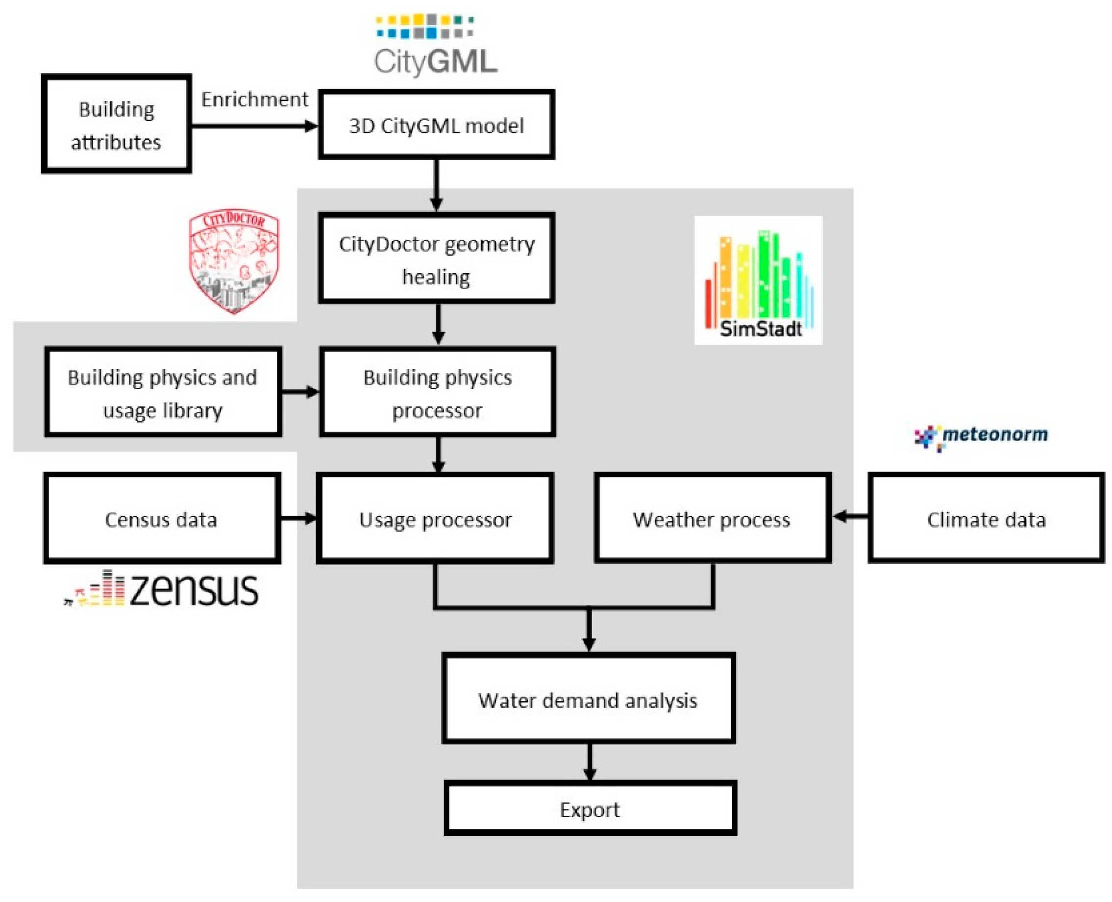
The water demand workflow is implemented within the simulation platform SimStadt, a platform under constant development at HFT Stuttgart [28]. Figure 1 shows inputs and calculation steps of the water demand workflow on a high-level step.

The CityGML data format that serves as basic inputs can depict existing environments such as buildings, roads and landscape. Building models are available in five Levels of Detail (LoD), with LoD 0 relating to a planar shape, LoD1 to data where buildings are represented as building blocks with average building height and a flat roof, LOD2 which has more detailed information about building heights and roof shapes, LoD3 introducing windows and LoD4 featuring information on ground plans and wall thicknesses [3]. The building function, e.g., residential, office etc., and year of construction is attached with CityGML as the basic input for the simulation. Building function decides in which calculation process the building should be directed to. Year of construction of residential determines the distribution of household sizes in terms of flat area and family size from census data.

The CityGML model is quality-checked by the tool CityDoctor [29], which can repair possible geometrical errors, e.g., open polygons, which prevent the buildings from being recognized properly. The model can then be stored in the CityGML 3D City Database (3DCityDB) geodata server or directly used for simulation in SimStadt [3].

The building physics library classifies buildings according to their type and year of construction. For each building type and period, there exists a typical building with its respective wall, roof and window properties. These properties are then applied to the actual building geometry for further calculation [30].

The usage library is based on several German norms and standards, focusing on heating set point temperatures, occupancy schedules and internal gains that are different according to the usage (residential, office, retail, etc.) of each building. To estimate the occupants in residential buildings, the usage library was extended with information on household size and number of occupants per household for all types of residential buildings based on the latest available German Census from the year 2011. The occupant numbers and the type of residential buildings (single family house or multi-family house) determines the water demand per capita as well as the total water demand.

The weather processor retrieves weather data of the geospatial location of the building model and creates synthetic hourly values for temperature and precipitation from monthly means in case only monthly data are available. Precipitation and temperature can have an impact on the water demand in residential buildings as well as some non-residential buildings [5,6]. The climate data are provided by Meteonorm, which generates representative typical years for any place on earth, including precipitation, temperature, irradiation etc., in hourly resolution [31]. The precipitation and temperature have impacts on water demand in residential buildings (Chapter 2.3), offices (Chapter 2.4.1) and hotels (Chapter 2.4.3).

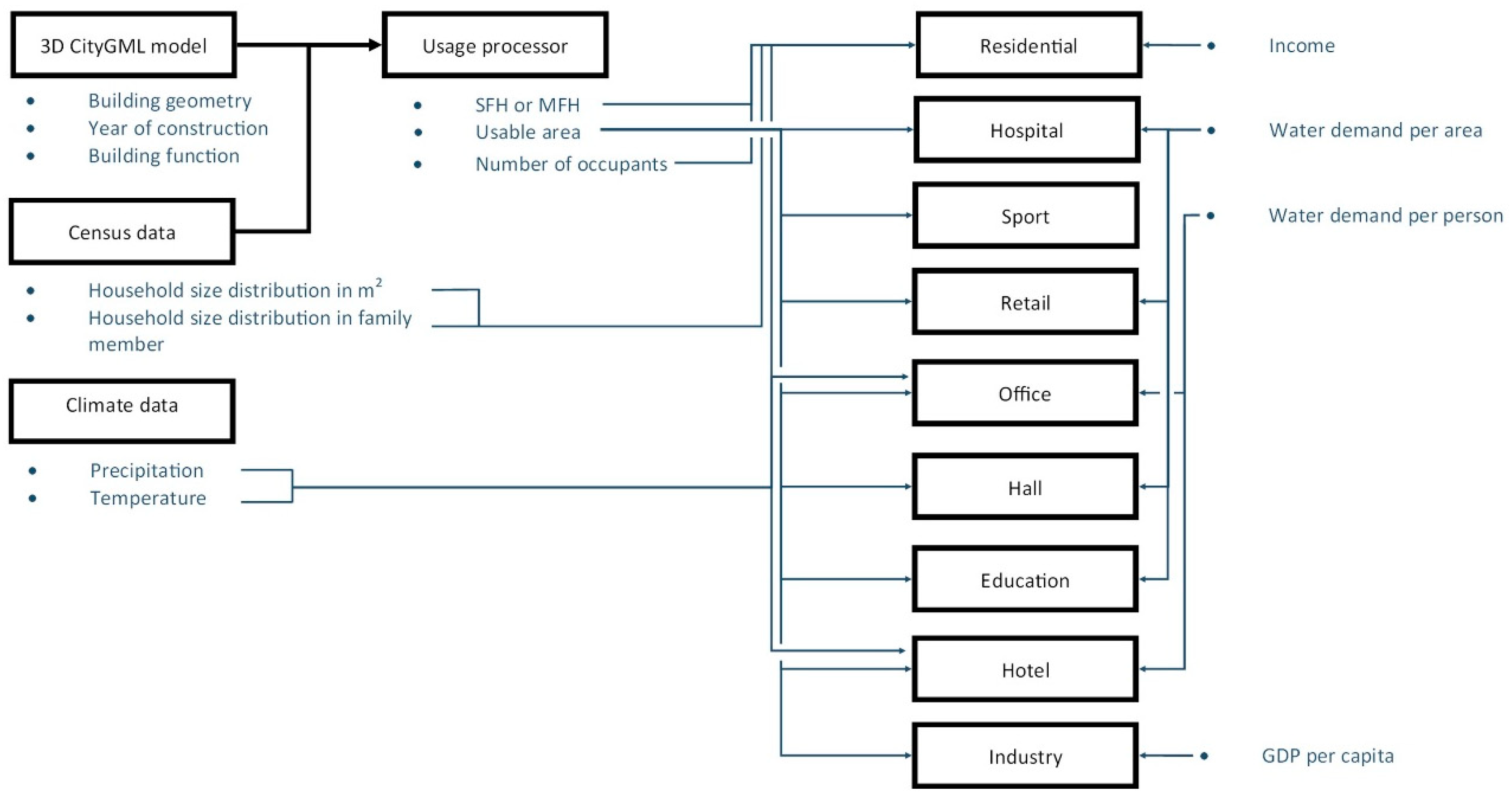
The information flow of Figure 2 shows the input data and data generated in intermediate steps, which are necessary for water demand calculation. Beside the information mentioned above, other necessary parameters are also included in the simulation, which are shown on the right side in the Figure 2. All the inputs generated and processed from the above-mentioned steps are passed on to the newly established water demand processor to estimating the water demand per building in the chosen region.

3.2. Building Volume and Heated Area Estimation

Given its wide and standardized availability, building geometric data are taken as one key input for the new workflow.

A building’s volume allows one to determine the number of residents or users. To determine the building volume, at least an LoD1, preferably LoD2, model is required. An LoD2 model has more details, e.g., attic, which increases the accuracy of the simulation. Each polygon of the building geometry is defined by a sequence of points in counterclockwise order. Volume calculation is integrated as part of a geometry processor in SimStadt [29]. If the data model is LoD2 or LoD3 (there is no information about internal structure of the building), it is assumed that the building has one thermal zone per story, internal ceilings are added to the model and the air volume is reduced by the volume occupied by these surfaces. Information related to cellar can be externally provided: if the cellar exists and, in that case, if it is conditioned or not. If this information is not provided, it is assumed that there is no cellar and, therefore, the floor is in contact with the ground. The attic is assumed to be ventilated but not heated unless other information is externally provided [32].

As the building volume calculation process mentioned before only calculates the heated area, the area is derived from the heated volume is heat area. The heat area is calculated according to Equation (1). Traffic areas such as entrance areas, stairwells, elevators and corridors are assumed to be heated. Technical areas (heating room, machine rooms, technical operating rooms), cellar and unheated attic are not included. The building heated area $A^N$ in m² is calculated in residential buildings as below:

$$A^N=0.32\frac{1}{m}{V}_e$$

(1)

where $V_e$ is the calculated building volume in m³.

If the average story height of a residential building, measured from the surface of the floor to the surface of the floor of the story above, is more than 3 m or less than 2.5 m, the useful floor area of the building shall be determined as Equation (2), notwithstanding the formula above:

$$A^N=\left(\frac{1}{h^G}-0.04\frac{1}{m}\right)V_e$$

(2)

where $h^G$ is the story height in meters [33].

3.3. Occupant Number Estiamtion and Water Demand in Residential Buildings

The water demand of residential buildings is usually given as the value per occupant [10,14,23,26]. To assess the occupant number, this paper uses a method for linking CityGML building models with 2011 census data [34] to obtain information on household size and number of occupants per household for all types of residential buildings. Based on the floor area described in Section 3.2, this step assesses the number of occupants and households in buildings for the next analysis. The information related includes: (1) single-family houses only have one household with its number of occupants; (2) the occupant numbers per household/dwelling in all multi-family houses. The latter method is subject to ongoing research and an upcoming publication [35].

Schleich et al. [5] econometrically analyze the impact of several economic, environmental and social determinants on per capita water demand in about 600 water supply areas in Germany. Besides price, income and household size, the effect of population age, the share of houses with wells, house type, precipitation and temperature are considered.

Household water demand is a composite of the direct demand for drinking purposes and demand for activities such as cooking, cleaning, washing, personal hygiene and gardening [36]. The extent to which water demand responds to changes in prices depends on whether water is used for necessities (e.g., to cook) or non-necessities (e.g., to wash cars).

In this research we take the method from Schleich et al. [5] to estimate water demand in residential buildings. Among all the influencing factors, few factors more related to this paper are chosen, including the price for fresh water and sewage (EUR/m³), average net income per capita (EUR), number of household members, house type (single family house (SFH) or multi-family house(MFH)), number of days with rainfall > 1 mm in summer months and average temperature in summer month into consideration. Only share the households with wells is not relevant to this paper and for individual household/building the statistical data of having wells is not available.

A log-log model, where all parameters enter the regression equation in logarithmic form, is used. The unit and definition of each parameter are shown in

Table 1. Parameters impacting water demand and mean, minimum and maximum values for Germany on county level. Source: [5].

Variable	Definition	Unit	Mean	Min.	Max.
WATER	Average water demand per capita per day	[Liters]	128.47	67.90	228.70
PRICE	Price for fresh water and sewage	[€/m3]	3.79	1.99	7.10
INCOME	Average net income per capita	[€]	16,541	12,735	21,893
SIZE	Average number of household members	[Number of persons]	2.03	1.49	3.66
AGE	Average age of population	[Years]	42.19	36.40	47.40
WELLS	Share of households with wells	[%]	1	0	20
ONEFAM	Share of single-family houses	[%]	51	26	91
RAINDAYS	Average number of days with rainfall > 1 mm in summer months 1	[Number of days]	7.90	5.00	10.80
TEMP	Average temperature in summer months 1	[Celsius]	16.72	13.10	19.80

¹ Summer months: April to September.

. The log–log model allows parameter estimates to be directly interpreted as elasticities of demand. However, one drawback is that the model it presumes these elasticities to be constant over the entire range of the variables. The regression equation for the water demand per capita and day in a log-log model is then given as:

$$\begin{array}{c}water={\beta }_{1}price+{\beta }_{2}income+{\beta }_{4}size+{\beta }_{5}age+{\beta }_{6}wells+{\beta }_{7}onefam+\\ {\beta }_{8}raindays+{\beta }_{9}temp+Stat{e}_i+constant+{\mu }_0,\end{array}$$

(3)

Lower case letters indicate that variables are in natural logarithmic form. ${State}_i$ is associated with federal states (of Germany), which is also relevant here: Germany’s five “new” eastern states, excluding Berlin, have average demand of 95 liter per capita per day and by this around 20% less water demand per capita and day than the “old” western states [5,37]. To reflect this difference, a correction value for each federal state is applied. Furthermore, ${\mu }_0$ is the error component which is not given in the result. Values for ${\beta }_i$ and ${\mu }_0$ in (3) are assessed by Ordinary Least Squares (OLS) to find the best fit for the data input, which contains 592 samples in Germany. The result is shown in

Table 2. Estimation results for water demand for the log-log model with the sample size of 592. Source: [5].

Variable	Elasticity β	Standard Error
Price	−0.242	0.058
Income	0.355	12.724
Size	−0.436	0.179
Age	0.603	0.329
Wells	−0.014	0.006
Onefam	0.073	0.065
Raindays	−0.147	0.088
Temp	−0.047	0.164
Constant	−146.83	62.121

.

Since our method accesses water demand of each building, whereas the parameter “ONEFAM” represents the percentage of single-family houses among all the residential buildings statistically in an area, the parameter “ONEFAM” should be simplified to a binary variable, with one value for a single-family house and one for a multi-family house. In the case water demands for multi-family house are to be assessed, it is assumed that the area under consideration consists only of multi-family house, with “ONEFAM” equal to 0. Since logarithms do not allow for 0 as value, the maximal and minimal values of the component ${\beta }_{7}onefam$ based on the maximal and minimal value of ONEFAM are calculated and then extrapolated linearly to the case {ONEFAM = 0; ONEFAM = 1}. The values of ${\beta }_{7}onefam$ in both extreme cases are listed in

Table 3. Estimation results for per capita daily water demand for the log-log model.

Value of ONEFAM	Method	Value of ${\mathit{\beta }}_7 \mathit{o}\mathit{n}\mathit{e}\mathit{f}\mathit{a}\mathit{m}$
1	Linear extension	0.00250929
0.91 (Max. in the real data)	Direct logarithmic calculation	−0.00298998
0.26 (Min. in the real data)	Direct logarithmic calculation	−0.04270695
0	Linear extension	−0.05859373

. As the parameters indicate, single-family houses can be expected to have higher water demands than multi-family houses, which is plausible, given the presence of gardens and their occasional irrigation in summer months.

Thus, the formulas for calculating the daily per capita water demands in residential buildings in single-family house (SFH) and multi-family house (MFH), respectively, are:

$$\begin{array}{c}wate{r}_{SFH,O}=0.054932-0.242price+0.355income-0.436size+\\ 0.603age-0.014wells-0.147raindays-0.047temp+State,\end{array}$$

(4)

$$\begin{array}{l}wate{r}_{MFH,O}=-0.0857-0.242price+0.355income-0.436size+0.603age\\ -0.014wells-0.147raindays-0.047temp+State,\end{array}$$

(5)

3.4. Water Demand in Non-Residential Buildings

The water demand simulation in non-residential buildings takes the floor area as the main building attribute. Literature data for area-specific water demand are available for hospital, sport halls, retail and educational buildings [6,14,38,39]. For offices and hotels, occupant numbers for a certain floor area serve as basis for assessing water demands. Regarding the limits of a generic method on water demand modelling for exhibition halls and industry, area specific water demand values are derived from the total amount of water demand in Germany or single states and their total floor area, respectively. The water demand values per square meter in hospitals, sport facilities, retails, halls and education facilities are directly taken from literation, indicated in

Table 4. Key parameters of water demand assessment in non-residential buildings.

Building Type	Floor Area per Occupant	Daily Water Demand per Occupant	Annual Water Demand
Unit	[m2/p]	[liter/person]	[m3/(m2 a)]
Hospital			$1.01+\frac{7.693}{\mathrm{Floor}\mathrm{Area}}$ [14]
Sport			0.279 [38]
Retail			1.1315 [6]
Office and Administration	14 [39]	96 (per working day) [6]	1.7
Hall			0.05 [40]
Education			3 [41]
Hotel	19 [42]	323 [6]	1.9
Industry			96 [43,44,45]

.

3.4.1. Water Demand in Offices

For offices, a workplace typically requires 8 to 10 m², including furniture and a proportionate amount of traffic space, according to existing guidelines. For open-plan offices, in view of the greater need for traffic space and possibly greater disruptive effects (e.g., acoustic, visual), a space requirement of 12 to 15 m² per workplace is to be assumed [39]. Water demand per occupant per working day is 96 liters [6], with a typical assumption of 250 working days per year.

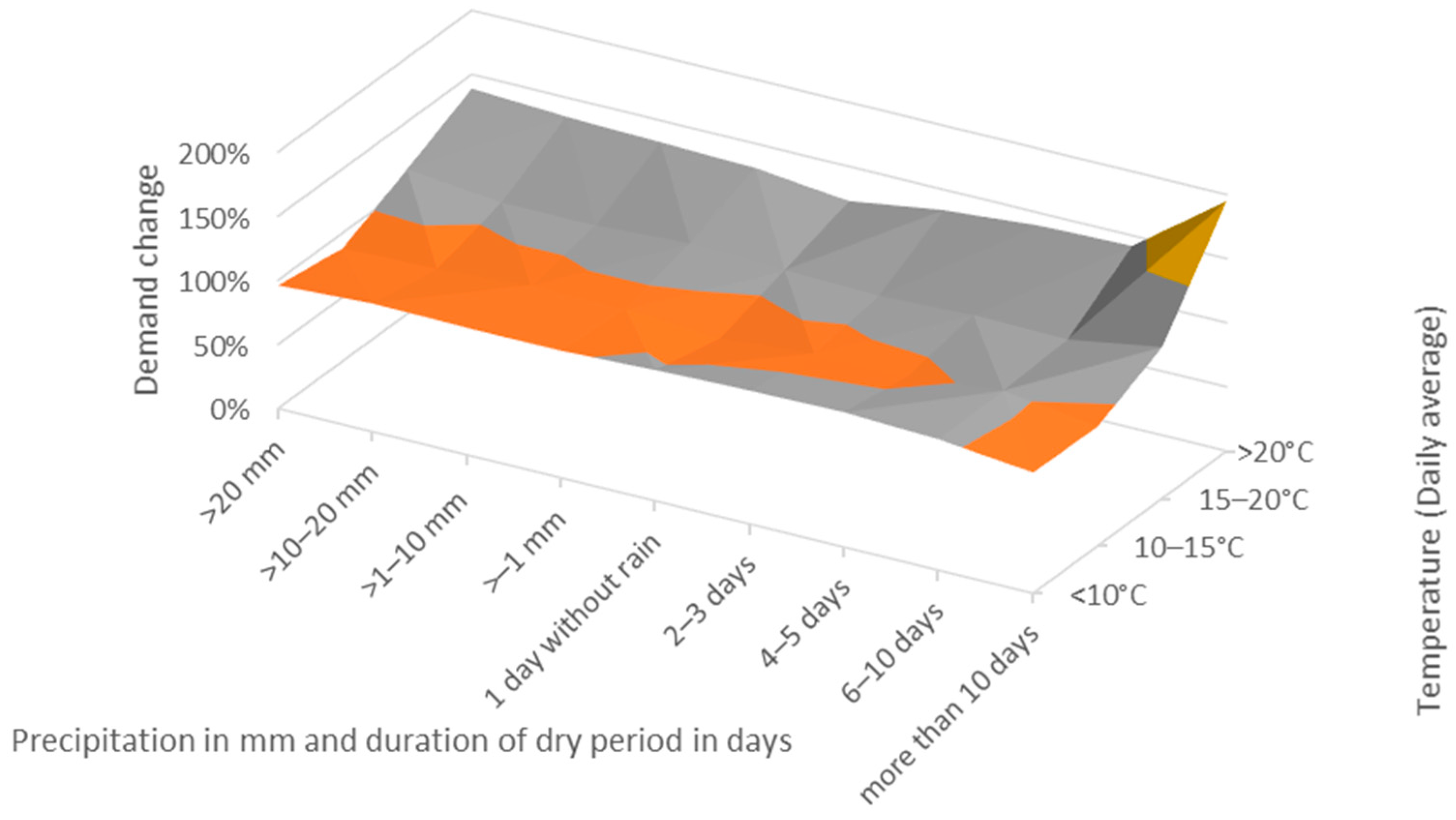
As Figure 3 indicates, water demand (including water for cooling) increases in summer with higher temperatures, with demand of drinking and process water for WC flushing decreasing, which dampens the total increase. The increase in water demand with rising daytime temperatures by up to 40% can be attributed to air conditioning systems [39].

3.4.2. Water Demand in Educational Buildings

Educational buildings are specified as a separate building category in the CityGML data. In the following

Table 5. Water demand per square meter and year in buildings for educational purposes. Source: [41].

Building Type	Unit	Water Demand
Social sciences	[m3/(m2 a)]	0.5–0.8
Nature sciences with medium amount of technical facilities (e.g., physics, electrical engineering)	[m3/(m2 a)]	2.0–4.0
Natural sciences with high amount of technical facilities (chemistry, biology)	[m3/(m2 a)]	4.0–7.0

, a water demand assumption of 3 m³/m² a is assigned for educational buildings.

3.4.3. Water Demand in Hotels

Hotel facilities usually consist of guest rooms, a lobby, breakfast/restaurant room, spa/wellness room, administration rooms and more. Differences in floor area, especially with regards to the guest rooms, exist between hotel categories. For a mid-tier hotel, for example, 25 m² usable floor space incl. bathroom is a reference value per room. Adding to this the proportional share for lobby, conference facilities etc. result in total floor space per room. For example, the above-mentioned hotel with a room size of 25 m² would have a total floor space of about 37.5 m² if corrected for public space. Generally, the resulting net floor area can be roughly achieved by an area surcharge of about 1/3 [42]. In the following, we use the net floor area of the middle-class hotel as the standard case.

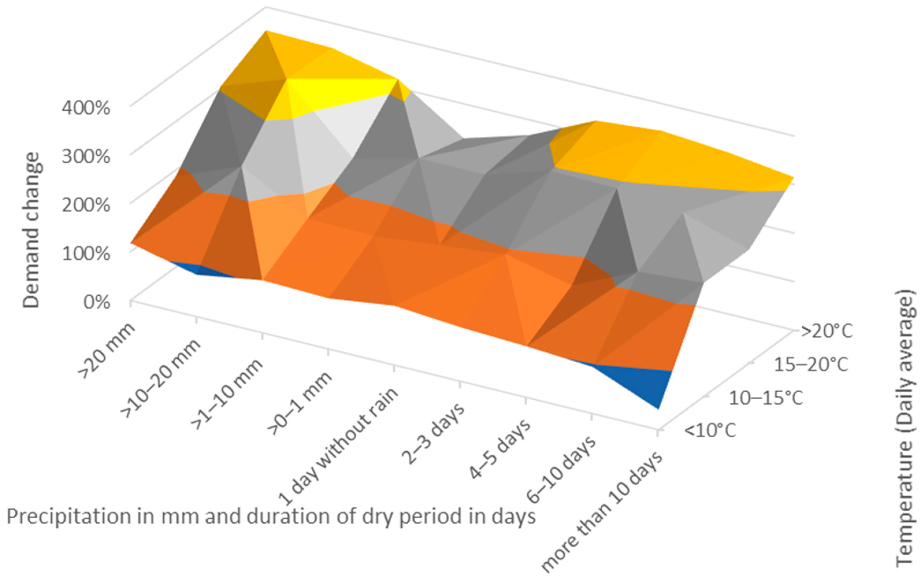
The average hotel occupancy rate in western Europe was 63.6% in 2019, which was still unaffected by the COVID-19 crisis [46]. We assume all hotel rooms are double rooms with two occupants, with a water demand per day of 345 liters [6]. The climatic situation, especially with regards to precipitation and temperature, which influence water demands, is considered. The impact by precipitation and temperature to water demand in hotels is shown in Figure 4.

Total hotel water demand increases with average daily temperatures, due to the fact that occupancy rates increase in summer. Furthermore, water demand also increases with rising precipitation levels, potentially due to an increased use of wellness/spa facilities under rainy weather. Likewise, an increase in demand can be observed in connection with persistent dryness, especially on the warmer days. Here, an increasing irrigation of outdoor facilities may be of importance.

3.4.4. Water Demand in Industry

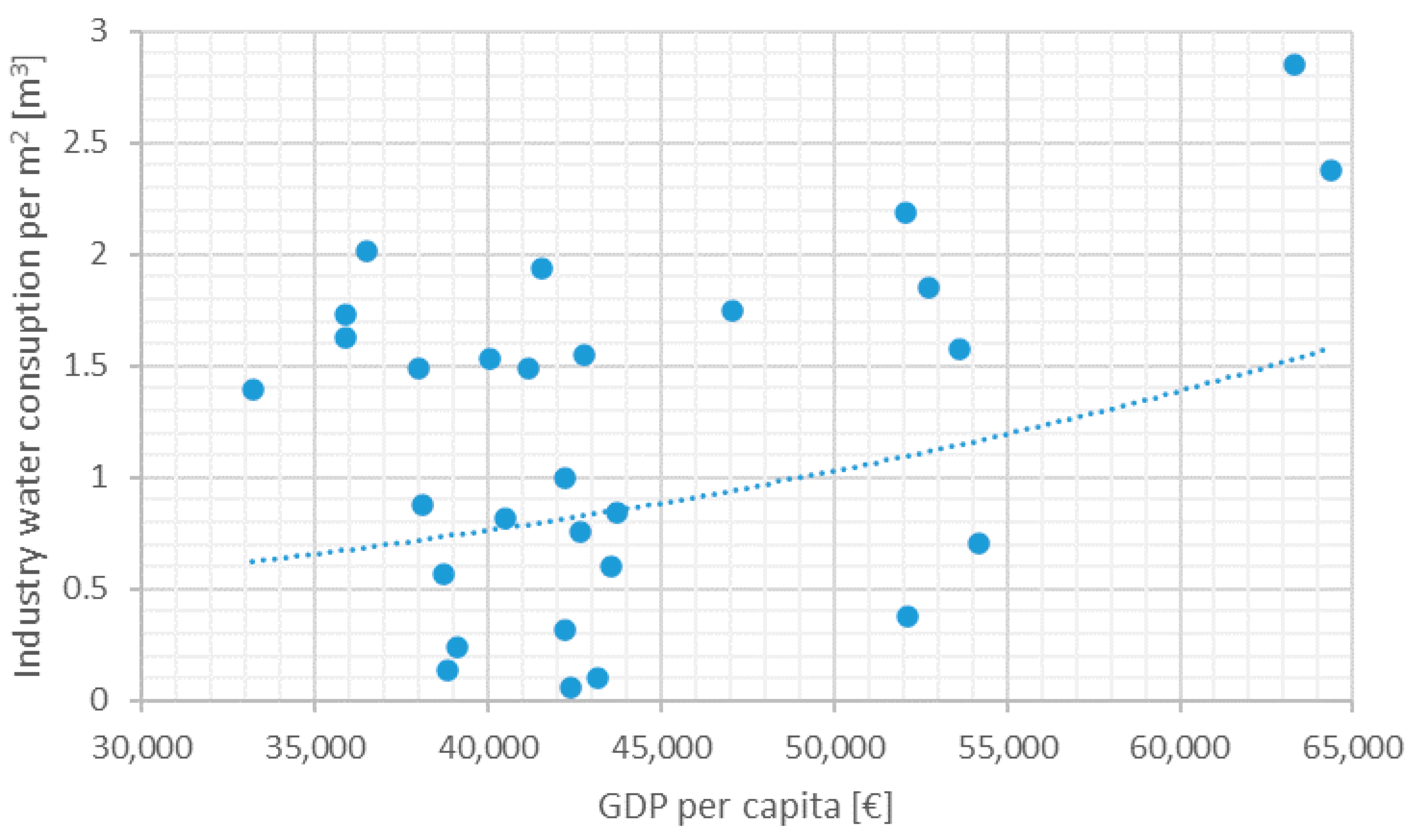
Overall water demand and yearly water demand patterns in industry of course differ very much with the type of industry under consideration—to give just one example, a warehouse will have a much lower water demand in almost all circumstances than a brewery or food processing plant. However, CityGML data do not specify which type of industry an individual industrial building belongs to. Regarding water intensity, cross-temporal and cross-regional data suggest that as GDP per capita increases, many countries follow a pattern of decreasing water demand per industrial value add [47]. This finding suggests that industrial water demand can be linked to local economic conditions as indicated by GDP per capita, available through census data (Figure 5). Therefore, the overall water demand in industry, GDP per capita and ground area used by industry in the three federal counties assessed here, located in the states of North-Rhine-Westphalia, Baden-Württemberg, Thuringia, were analyzed. Data were obtained from each State Bureau of Statistics [48,49,50]. As data on industrial floor area at state level are not available, industrial ground area is taken as an approximation. Performing a regression analysis, the Pearson’s correlation coefficient between GDP per capita and industrial water demand is 0.62, a moderate strength of relationship (strong > 0.7, moderate 0.4–0.6, weak < 0.4 [51]). Of course, industrial water demand is defined by many other factors than GDP, most importantly the type of industry. Given the level of information contained in CityGML, a correlation with per capita GDP is, however, widely applicable.

3.5. Validation

As mentioned earlier, three German counties with different climatic and socio-economic conditions were used to validate the feasibility, accuracy and resilience of the established water demand workflow. The city of Cologne (North-Rhine-Westphalia) represents a densely populated urban area, while the county of Ludwigsburg (Baden-Württemberg) represents a typical southern suburban area and the county of Ilm-Kreis (Thuringia) a more rural region that is in many dimensions close to the average German county outside of large metropolitan areas. Key socio-economic and climatic data for the tree counties between 1995 to 2015 are listed in

Table 6. Socio-economic and climatic data of the three German counties used for validation.

Parameter	Unit	Ludwigsburg	Ilm-Kreis	Cologne
Average age [52]	[Years]	42.1	45.6	42.4
Annual net income [53,54]	[€/person]	17,244	13,847	15,984
Water price	[€/m3]	5.37 [55]	4.03 [56]	3.16 [57,58]
Longitude	[°]	9.150	10.948	6.958
Latitude	[°]	48.900	50.757	50.937
Average altitude	[m]	302	421	57
Yearly average temperature	[°C]	10.1	8.7	12.0
Precipitation	[mm/a]	729	602	811
Percentage of flats in buildings with living space less than 40 m2 [59]	[%]	4.1	6.1	10.2
Residential floor area per capita	[m2]	43 [60]	46 [61]	39 [62]
Population density [33]	[Person/km2]	792	136	2168

.

Table 7. Key validation results.

Variable	Unit	Ludwigsburg			Ilm-Kreis			Cologne
		Si 1	St 1	Di 1	Si 1	St 1	Di 1	Si 1	St 1	Di 1
Water demand of residential buildings	[1000 m3/a]	16,619	14,176	17%	5360	3607	49%	39,573	60,301	−34%
Water demand per capita	[L/(dp)]	113	114	−1%	97	90	7%	147	154	−5%
Water demand of non-residential buildings, excluding industry	[1000 m3/a]	3278	3116	5%	682	1604	−57%	12,106	11,920	2%
Water demand of industry	[1000 m3/a]	36,744	-	-	88	361	−76%	145,349	56,377	158%
Industry building area	[ha]	-	-	-	133	1233	−89%	36,835	15,378	140%
Water demand of residential buildings after scaling	[1000 m3/a]	14,982	14,176	6%	3848	3607	7%	57,342	60,301	−5%
Households	[1000–]	174	152	15%	77	55	40%	418	515	−19%
Residents	[1000–]	392	353	11%	152	109	39%	738	1070	−31%
Residential floor area	[ha]	-	-	-	666	489	36%	2873	3809	−25%

¹ Simulation (Si); Statistic (St); Difference (Di).

shows the results of the newly established water demand workflow, including household and occupant number as well as water demands per different sectors for the three aforementioned counties. Comparing the estimation result with the statistical number from German Census 2011 data [63,64], the model yields differences (to statistical data) from 15% to 40% for the number of households, and 11% to 31% for the number of residents. Since the household estimation model introduced in Section 3.3 uses average German household floor areas and an average number of occupants per household, our modeling results are more accurate in areas with a mid-sized population density such as Ludwigsburg, which are close the German average value. In rural areas, e.g., Ilm-Kreis, a house with relatively large floor areas is usually occupied by fewer occupants than on average (in Germany), leading to an overestimate of the number of households and their population. Similarly, in densely populated cities, such as Cologne, the floor area per household is typically smaller and at the same time the number of occupants per dwelling is higher than indicated based on German average statistical data (Table 6). Thus, our workflow simulation yields around 19% less households and 31% fewer resident number.

In terms of water demand per capita in residential buildings, numbers calculated by the newly established workflow deviate by between 1% and 7% from the statistical value. It has to be noted that the residential water demand given by North-Rhine Westphalia’s statistical office for Cologne includes small business units, which explains higher values than the simulation result. At a county and city level, the result of residential water demand per capita tends to be accurate compared with statistical data. If the error is eliminated by scaling the aggregated residential water demand in each region with the same ratio resident number difference, the gap between simulation result and statistical value narrows to between 5% and 7%.

Statistically, the value for water demand in non-residential buildings is the difference between the total public water supply to end users and water supply to households. As more detailed data on water demand per building category, e.g., retail, school and etc. are not available, validating the accuracy of the water demand output of individual building types in the newly established workflow against statistical data is difficult. We assume that the building types including office, hospital, retail, sport facility, hall, education and hotel, source all their water from the water utility, i.e., self-extraction is assumed to be zero. In that case, water demands in Ludwigsburg and Cologne deviate by 5% and 2%, respectively, from derived statistical data, shown in Table 7.

Larger differences in water demand in industry in the studied counties result from errors in building function assignment in the CityGML. For example, 1100 ha out of a total of 1233 ha of industrial area are missing for Ilm-Kreis, whereas the industrial floor area in Cologne seems to be overestimated by 35,000 ha, which in reality seem to be residential areas. On top of this, water demand in industry differs from region to region as mentioned Section 3.4.4. However, water demand per floor area is estimated in all regions at the same magnitude according based on regression analysis.

It can thus be seen that the accuracy and quality of the CityGML data plays an important role in the accuracy of water demand assessments, with missing building functions and errors in building geometries yielding up to 36% in difference in residential building floor area estimations, and missing buildings in the data model resulting in lower water demand than statistically assessed.

3.6. Scenarios and Location Setting

As stated in the end of last section, a well-validated CityGML data file of the village of Rainau (Baden-Württemberg) is used for a scenario study [65]. It has a population of 3318 and a land area of 2547 ha. Of this, 75 ha are used for residential living and 23 ha for industry [66].

Table 8. Scenarios setting for Rainau, Baden-Württemberg, Germany.

Scenario	Climate	Average Age [Years] [67]	Water Price [€] [68]
1	Average history data in year 2000–2010	38.9	4.89
2			5.42
3		43.3	4.89
4			5.42
5	Predicted in year 2030	38.9	4.89
6			5.42
7		43.3	4.89
8			5.42

indicates the three parameters used for creating different scenarios, which are related to the parameters stated in Table 1: climate, average age, water price. Average historic climate data for 2000–2010 and predicted climate data in 2030 were taken from Meteonorm (precipitation and ambient temperature). Age represents the average age of the population, which is 38.9 in Rainau compared with the German average of 43.3. The water price includes fresh water supply as well as wastewater disposal and treatment cost per cubic meter.

4. Results of Scenario Analysis

Table 9. Simulation results of case study Rainau.

Scenario	Residential Water Demand	Residential Water Demand per Capita	Non-Residential (Excluding Industry) Water Demand	Industrial Water Demand
Unit	[1000 m3/a]	[L/p d]	[1000 m3/a]	[1000 m3/a]
1	174.2	102.6	192	397
2	169.9	100.1	192	397
3	185.8	109.5	192	397
4	181.2	106.8	192	397
5	173.5	102.3	194	579
6	169.3	99.8	194	579
7	185.1	109.1	194	579
8	180.6	106.4	194	579

shows the water demand simulation result of all eight scenarios in Rainau as defined in Table 8. The result is based on the assumptions that (1) The total number of inhabitants is constant across these eight scenarios since the same CityGML file is given and the distribution function of occupant estimation algorithm is not changed; (2) the water demand pattern is based on the data collected in the past. The change of water demand pattern in the future is not forecasted in this study.

As with the nature of Equations (2) and (3), the higher the average number of days with rainfall exceeding 1 mm in the summer, the lower the water demand, due to reduced water demand for gardening [5]. In contrast, increasing summer temperatures is statistically a less significant influencing factor on water demand, since the absolute value of elasticity is the lowest of all (see Table 2).

Comparing scenarios 1–4 against scenarios 5–8 residential water demand in 2030 decreases by around 700 m³/a, or 0.4%, compared with demand based on the current climate.

Table 10. Climate in summer months (April to September) during 2000–2010 and 2030 in Rainau.

Month	Ambient Temperature [°C]		Precipitation [mm]
	2000–2010	2030	2000–2010	2030
Apr	10.0	9.8	43.0	56.0
Mai	14.7	14.4	82.0	77.0
Jun	18.1	17.4	79.0	90.0
Jul	19.1	19.5	88.0	88.0
Aug	19.0	19.2	78.0	82.0
Sep	14.6	15.8	58.0	62.0
Annual average	10.1	10.5	247.0	248.0

shows the climate in Rainau, in terms of precipitation and temperature in summer months. As in Equation (3), only the summer climate and precipitation have an impact on residential water demand. The climate is shown in two cases—the historical average between year 2000 and 2010 and the forecast value in year 2030. While in April, May and June, average temperatures in Rainau will increase by 0.7 °C (indicated in Table 10), the weather data predict more rainfall in the summer in this region, which overcompensates additional water demands due to rising temperatures.

Furthermore, the results show an ageing society can lead to higher residential water demand. If the average age increases by 4.4 years, as indicated in Table 8, per capita water demand increases by about 6 liters per day. Water demand may increase with age because retired people spend more time at home and gardening [5]. The data from a recent survey of energy use patterns from more than 20,000 households in Germany and show that older people take fewer showers and more baths, corroborating our findings [69].

Lastly, increasing the water price from EUR 4.89 to EUR 5.42 per m³, per capita water demand in the residential sector drops by between two and three liters per day. Combing the influences brought by climate in 2030 and aging of the population, residential water demand per capita will increase from 102.6 L/d to in scenario 1 to 109.1 L/d in scenario 7. Scenario 7 is the most likely situation in the future. In order to limit the residential water demand, the possible solution would be to increase the water and wastewater price. By raising the water price from EUR 4.89 to EUR 5.42 per m³, the per capita water demand in the most likely scenario in the future will go down to 106.4 L/d in scenario 8 from 109.1 L/d in scenario 7.

The water demand calculation in non-residential sector, excluding industry, lacks the linkage with the socio-economic parameters; only changes in climate data have an influence on non-residential water demand in the scenarios presented in Table 8 (excluding industry). Considering an annual average temperature increase of 0.4 °C, and annual precipitation remaining (almost) constant, non-residential water demand (excluding industry) increasing from 192 m³/a to 194 m³/a.

In the workflow, industrial water demand is only related to the local economic situation, represented by GDP per capita. According to the forecast of the German Federal Ministry of Transport and Digital Infrastructure, GDP per capita will grow by 14% between 2020 (EUR 42,709 per person) and 2030 (EUR 48,689 per person) [70]. By this, Rainau’s industrial water demand increases by 200 m³/a in Rainau 46% between 2020 and 2030.

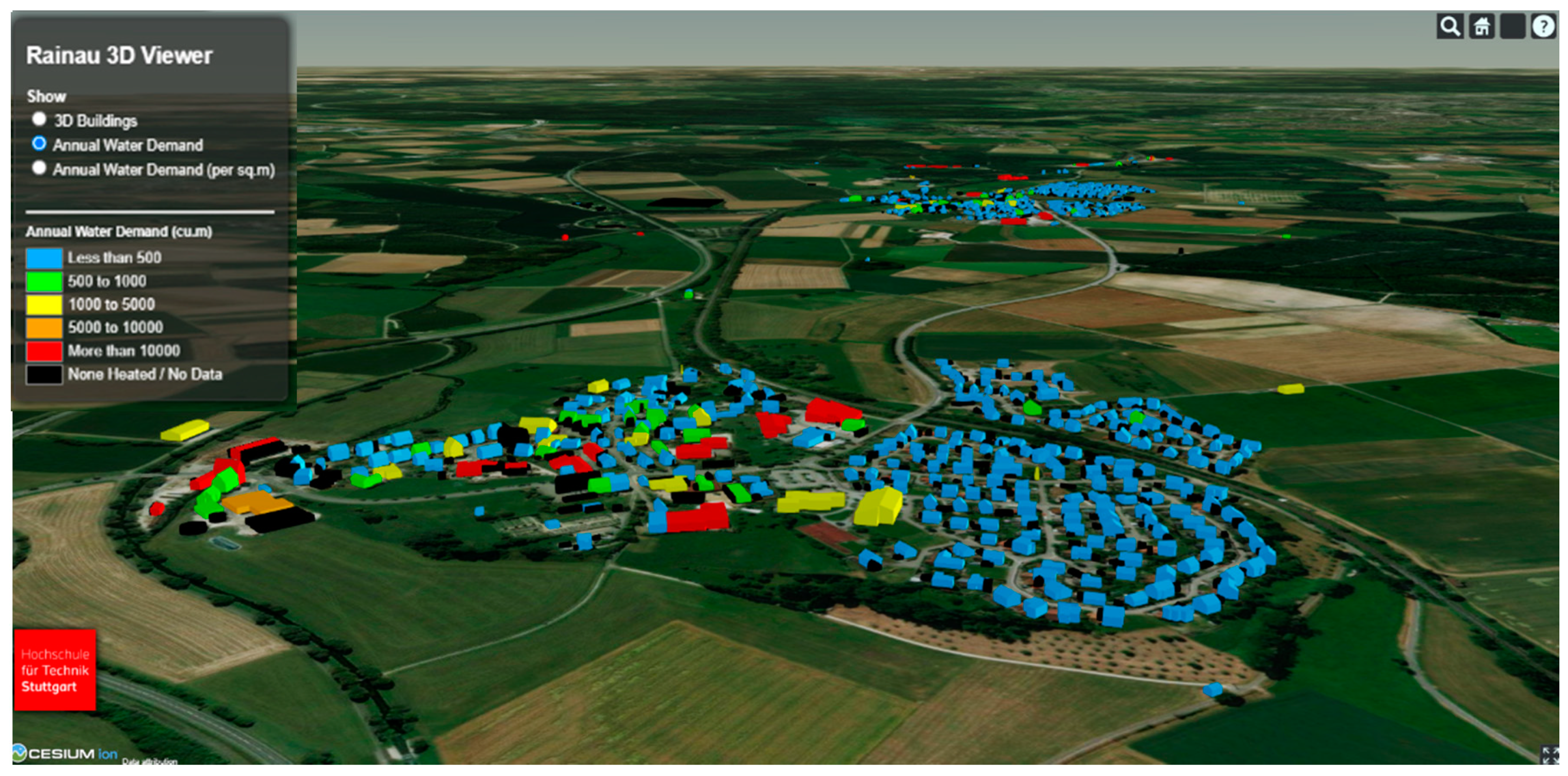
The above-mentioned results were combined with CityGML data for visualization in the web framework CesiumJS, using 3D Tiles. Figure 6 shows the total water demand of each building in Rainau of the default scenario: buildings in blue have water demands of less than 500 m³ per year, with most single-family houses belonging to this category. Buildings in green are mostly multi-family houses, a few single-family houses and office buildings with annual water demand between 500 and 1000 m³. Most office buildings, all sport halls and schools belong to the yellow and orange category with annual water demand between 1000 and 10,000 m³. Industrial buildings with the highest water demand per buildings, above 10,000 m³, are colored in red.

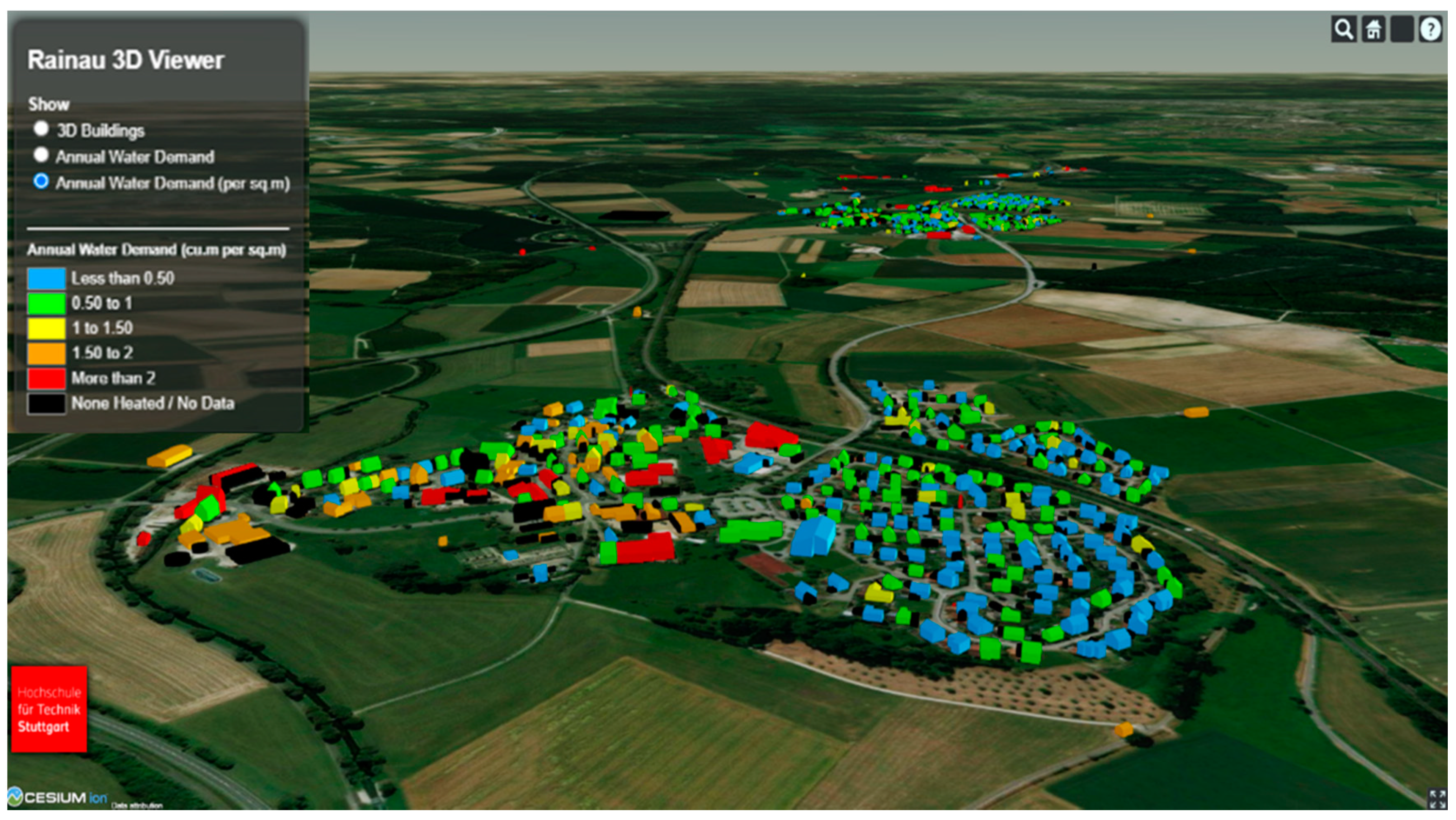
Figure 7 does not give the total water demand, but water demand per floor area. Residential buildings have water demands per square meter below 1.5 m³ per m² and year (in blue, green and yellow), with a few single-family houses in blue having values per m² below 0.5 m³/m². As occupants in single-family houses have more living space per person, even though they consume more water per person the water demand per area in SFH is in the lowest category. In Figure 5 the sports hall located in the middle part in yellow has one of the highest absolute water demands (1455 m³/a); however, per square meter demand is among the lowest and below 0.5 m³/m². Due to lower values of floor area per resident than in single-family houses, multi-family houses have the highest water demand per square meter among residential buildings, peaking with some yielding more than 1.5 m³/m². Office buildings have the second-highest water demand category in orange between 1.5 and 2 m³/m² behind industrial building with values above 2 m³/m² in red. There is no difference between industrial buildings in term of water demand per area, as the identical specific water is applied to all industrial buildings in the same region.

5. Discussion

A newly established workflow with the function of water demand modelling in Germany was introduced to an existing urban energy simulation platform based on widely available CityGML models and standard statistical data as its key inputs. Next to being based on these data types, the uniqueness of the new workflow is to allow a resolution down to the single building, whereas existing water demand models focus more on the municipal (or even higher) levels. The annual water demand of individual residential households and non-residential buildings can be modeled and visualized in 3D.

The method fills the gap of assessing an individual building or city quarter’s water data based on CityGML, thus allowing assessments to be performed with a limited set of input data. In residential buildings, the workflow models water demand per occupant had a deviation from 1% to 7% from the statistic values for three German counties. With enough confidence, we argue that the simulation tool is reliable in terms of calculating per capita water demand and total water demand in residential buildings with the correct CityGML input data model. There is more uncertainty of water demand simulation in non-residential buildings. However, the magnitude of demand value is at the same level. This accuracy is realized by considering local climate and some socio-economic factors. More importantly, the modelling process is fully automated, at least for Germany, but can be easily applied to other world regions, provided CityGML models and statistical data are available.

The workflow thus completes a gap in the analysis of regional food-water-energy nexus issues. For instance, a combination of its results with water demands from agriculture and local water availabilities allows us to assess the level of regional water stress and to define improved strategies for crop cultivation or water conservation in urban and rural areas. Such assessments can greatly help local governments to make strategical decisions on existing and new-built areas either in the current situation or in the future.

Because of the highly aggregated inputs, using values at country level, which might not always match the local situation, a certain level of uncertainty in the modelling results is added, e.g., using average German household size and occupancy rates. As a next step, local census data on key parameters should replace German average values, so that local resident number can be estimated more accurately, e.g., in dense urban areas.

The inaccuracy of building function can be eliminated by cross-checking CityGML with OpenStreetMap as OpenStreetMap is more frequently maintained by private users. Adding building function sub-classes of non-residential buildings can also improve the simulation accuracy, e.g., water demand in elementary school and university are distinctive, even though they are both classified under “education” in standard CityGML. Generally, limited statistical data are available on water demand of non-residential buildings. As a result, empirical values of water demand per area have to be taken from literature and studies focusing on the German national level. Adding on the German residential water demand method, the water demand simulation model is only restricted for the application in any city in Germany. Moreover, lacking water demand data in non-residential buildings makes the accurate validation of water demand in specific facilities difficult. This decreases the accuracy of the model. Here, a next step might be the gathering of relevant information from other sources to further improve modelling quality.