Soil Mapping Based on Globally Optimal Decision Trees and Digital Imitations of Traditional Approaches


1
V.V. Dokuchaev Soil Science Institute, 119017 Moscow, Russia
2
Ecological Faculty, Peoples Friendship University of Russia (RUDN University), 117198 Moscow, Russia
*
Author to whom correspondence should be addressed.
ISPRS Int. J. Geo-Inf. 2020, 9(11), 664; https://0-doi-org.brum.beds.ac.uk/10.3390/ijgi9110664
Submission received: 24 September 2020
/
Revised: 29 October 2020
/
Accepted: 2 November 2020
/
Published: 4 November 2020
Abstract
:Most digital soil mapping (DSM) approaches aim at complete statistical model extraction. The value of the explicit rules of soil delineation formulated by soil-mapping experts is often underestimated. These rules can be used for expert testing of the notional consistency of soil maps, soil trend prediction, soil geography investigations, and other applications. We propose an approach that imitates traditional soil mapping by constructing compact globally optimal decision trees (EVTREE) for the covariates of traditionally used soil formation factor maps. We evaluated our approach by regional-scale soil mapping at a test site in the Belgorod region of Russia. The notional consistency and compactness of the decision trees created by EVTREE were found to be suitable for expert-based analysis and improvement. With a large sample set, the accuracy of the predictions was slightly lower for EVTREE (59%) than for CART (67%) and much lower than for Random Forest (87%). With smaller sample sets of 1785 and 1000 points, EVTREE produced comparable or more accurate predictions and much more accurate models of soil geography than CART or Random Forest.
1. Introduction
Global Soil Map projects related to obtaining spatial soil information require new techniques for constructing soil maps that can use legacy data in digital soil mapping [1,2,3]. Digital soil mapping is the process of creating and populating geographically referenced soil databases generated at specific resolutions via field and laboratory observation methods coupled with environmental data through quantitative relationships [4]. This soil-mapping paradigm is based on the use of modelling methods for establishing the soil–landscape relationships needed to estimate the probability of soil occurrence or its properties described by environmental or remote sensing data [5,6,7,8,9,10].
The digital soil mapping paradigm is gradually replacing the traditional soil mapping paradigm; however, huge archives of traditional soil maps exist and were created by expert soil-mappers in accordance with the qualitative paradigm [5]. To completely utilize these archives, digital soil mapping approaches should consider the qualitative nature of these traditional soil mapping processes. When utilizing legacy soil maps, it is most beneficial to use statistical methods that provide pedological knowledge in a form close to traditional forms [11]. There should also be possibilities for extracting and exploiting traditional qualitative knowledge about spatial soil propagation in the statistical models in an objective form [12,13]. It is also important in digital soil mapping to adopt “sleeping beauty” ideas and techniques from the traditional processes of soil mapping [14].
In traditional soil mapping, the values of other products besides soil maps are often underestimated. This product involves explicit rules for the delineation of soil class units or soil properties. These explicit rules were formulated by soil-mapping experts and have rarely been expressed in their complete form. These rules were evaluated by experts to determine their notional consistency and have been used to predict soil trends and investigate soil geography and many other applications. For digital soil mapping, qualitative knowledge can be incorporated into quantitative soil models to yield more accurate soil maps in soil geography. For example, alluvial soils are associated with the floodplains of rivers, whereas organic soils are associated with swamps and marshes. In addition to these models, such expert qualitative information could provide substantial improvements in the accuracy of soil maps [15].
There are many soil mapping frameworks that are based on statistical methods and provide satisfactory prediction results: DSMART—resampled classification trees [16]; SoilGRIDs—Random Forest, multiple linear regression, and ensemble methods [7]; and DoSoReMi—Random Forest [17], among others. If a complete sample set is used for modelling, ensemble methods, such as a Random Forest, yield the highest prediction accuracy [18,19,20]. However, there are several basic limitations for obtaining accurate statistical models based on “pure” quantitative statistical approaches without using additional qualitative knowledge [21]. In addition, extrapolation issues exist due to a dependence on the quality of spatial sampling and over-fitting [20].
Few developments in digital soil mapping represent the soil mapping rules in an explicit form. One such approach uses SoLIM (Soil Land Inference Mode) technology, which is based on fuzzy logic [22,23]. This approach differs from the traditional method of formulating rules for soil mapping. In 2003, Qi and Zhu developed another approach for formulating tree-based rules like traditional soil mapping using the See5 algorithm [11]. Subsequently, this algorithm was integrated with the statistical fuzzy-logic approach [24]. Therefore, the SoLIM framework integrates many traditional methods for soil mapping, enabling the development of pedologically sound soil maps.
Most existing frameworks integrate only some traditional methods for soil mapping. However, the traditional process of soil mapping compilation can be imitated using the achievements of digital soil mapping. Many useful results could be obtained if the entire work process of a traditional soil mapper was imitated, including the process of soil map compilation via the cartographic methods used for covariate analysis [25]. In addition, there are approaches for incorporating expert knowledge into automatically created models, as well as extracting and transferring explicit knowledge [26,27,28].
New approaches enable the combination of expert-based knowledge and mathematical modelling to fuse the quantitative and qualitative descriptions of the relationships between soils and soil formation factors. Structural equation modelling (SEM) is a contemporary approach that facilitates the integration of knowledge about soils into a statistical model and provides an opportunity to assess the inter-relationships of various soil properties during modeling [21]. According to the authors, “It bridges the gap between empirical and mechanistic methods for soil–landscape modelling and is a tool that can help produce pedologically sound soil maps” [12]. However, the SEM approach is more aimed at incorporating expert knowledge than extracting knowledge from legacy data. Moreover, full theoretical models of SEM are presently more complex than simply representing practical rules for soil delineation in the traditional soil mapping process.
Another method of extracting the soil–landscape relationship is to use methods based on classification and regression tree algorithms. Representation with decision trees involves using the practical rules that were considered by the soil-mapping experts for soil mapping. Philippe Lagacherie implemented one of the most widely used methods, the classification and regression tree algorithm, for soil mapping in 1992 [29]. Feng Qi and A-Xing Zhu wrote a broad review about using the See5 algorithm to acquire knowledge for soil mapping [11]. Most of the classification and regression tree algorithms use locally optimal splitting criteria such as Gini or entropy for recursive stepwise partitioning [30]. These methods are aimed at obtaining satisfactory prediction accuracies but not at developing an optimal model. This leads to the substantial overlearning of a tree. Such a tree can be large and have poor notional consistency for some rules while yielding satisfactory prediction accuracy for the key site. These locally optimal methods include CART (Classification And Regression Trees), CTREE (Conditional Inference Trees), CHAID (Chi-square Automatic Interaction Detection), See5, and CUBIST (Rule- And Instance-Based Regression Modeling), along with many others [31]. Classification and regression tree algorithms of a new type have been proposed and aim at finding the optimal and most meaningful classification trees, e.g., evolution trees [31], neural decision trees [32], and deep neural decision trees [33]. Such globally optimal methods potentially allow much more meaningful knowledge to be obtained about the relationships between soil and soil formation factors.
Intrinsically, the methods for the extraction of soil–landscape relationships may only yield reliable models when the input data for modelling are available with good quality. In traditional soil mapping, soil mappers utilize a limited number of the most significant soil formation factor maps to formulate compact and comprehensive rules for soil delineation. The same strategy of using only meaningful covariates forms the basis of our approach that we propose for constructing meaningful statistical models that can be easily analyzed by experts [15,25,34]. In this study, we propose and evaluate a framework for constructing regional soil maps based on a digital imitation of traditional soil mapping and test this approach at a site in the Belgorod region of Russia.
2. Materials and Methods
2.1. Test Site
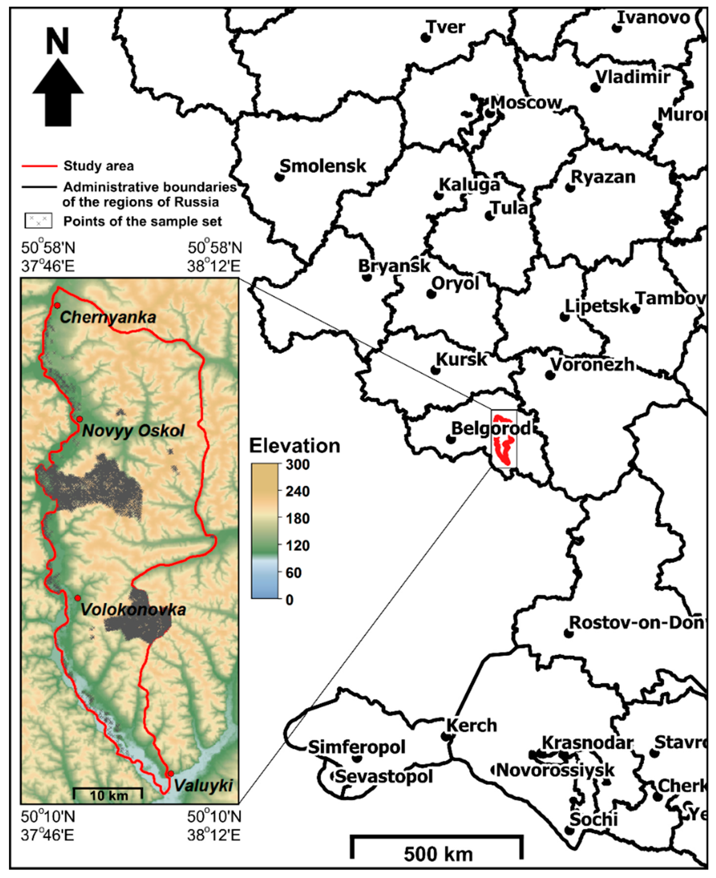
The test site is situated in the Belgorod region of Russia (Figure 1). The square size of the test site was 1560 km2. The coordinates of the corners of the study area are 50°10′ N, 37°46′ E, 50°58′ N, and 38°12′ E. Chernozems Pachic and Chernozems Albic are the dominant soils in the region. The terrain is a heavily dissected wavy-flat hilly plain. The parent materials are loess loam and clay, chalk sediments, alluvial and fluvioglacial sands, and sandy loams. The climate is continental with a hot summer and a moderately cold winter. The natural vegetation is represented by isolated oak and pine forests, meadows in dry valleys and floodplains, and calciphytic vegetation on steep slopes. However, croplands are dominant.
Large-scale soil maps created using the legend for the Russian classification of soils 1977—RCS1977 [35], were used as the basis for modelling. Further, translations were added to the modern Russian classification of soils 2004—RCS2004 [36] and the World Reference Base for Soil Resources 2006—WRB2006 [37].
The main relationships between soils and the soil formation factors are shown in the Table 1.
For the test site, a sample set with a mean distance of 120 m between key points was made using large-scale soil maps. In the Integrated Land and Water Information System (ILWIS) program, points were set randomly, and the soil classes from the traditional large-scale soil map were assigned to them. The sample-set size of 5001 points covered the central part of the study area and represented all soils (Figure 1). A distance of 120 m between points was chosen for the margins considering that one soil point should relate to the smallest possible soil polygon 2 mm by 2 mm in size on a traditional soil map at a medium scale of 1:200,000 [38,39,40]. The accuracy of the boundary positioning at this scale is the closest to the 90 m resolution of the covariates [41]. The whole approach for making the sample set was based on the classic method for the compilation of medium-scale soil maps. The smallest polygon on the map should be set using one soil pit or using information collected from a large-scale soil map.
2.2. Proposed Approach for Soil Mapping
The main strategy of the proposed approach is to use statistical methods and remote sensing data to imitate traditional soil mapping methods for the compilation of a regional scale soil map. Classification and regression tree algorithms were used to identify the relationships between the soil and soil formation factors in the form of an explicit decision tree model. This model was trained on the key sites in the soil region and then extrapolated to the area of the soil region where there was a lack of information about the soil. The obtained decision tree model can be traced and corrected manually. An appropriate statistical method was selected to find the optimal decision tree. The selected method was integrated into the digital soil mapping framework based on the stages of the traditional soil mapping process (Table 2).
A model for the delineation of soils was created for each soil region of the test area, in which the earth–landscape relationships between the ground and soil formation factors were considered the same. This strategy was used in traditional soil mapping (TSM) for soil features [11,38,42]. The soil region is defined as a lithologic–geomorphologic region with the same geological history. The regionalization was obtained based on landform or river watershed delineations [42].
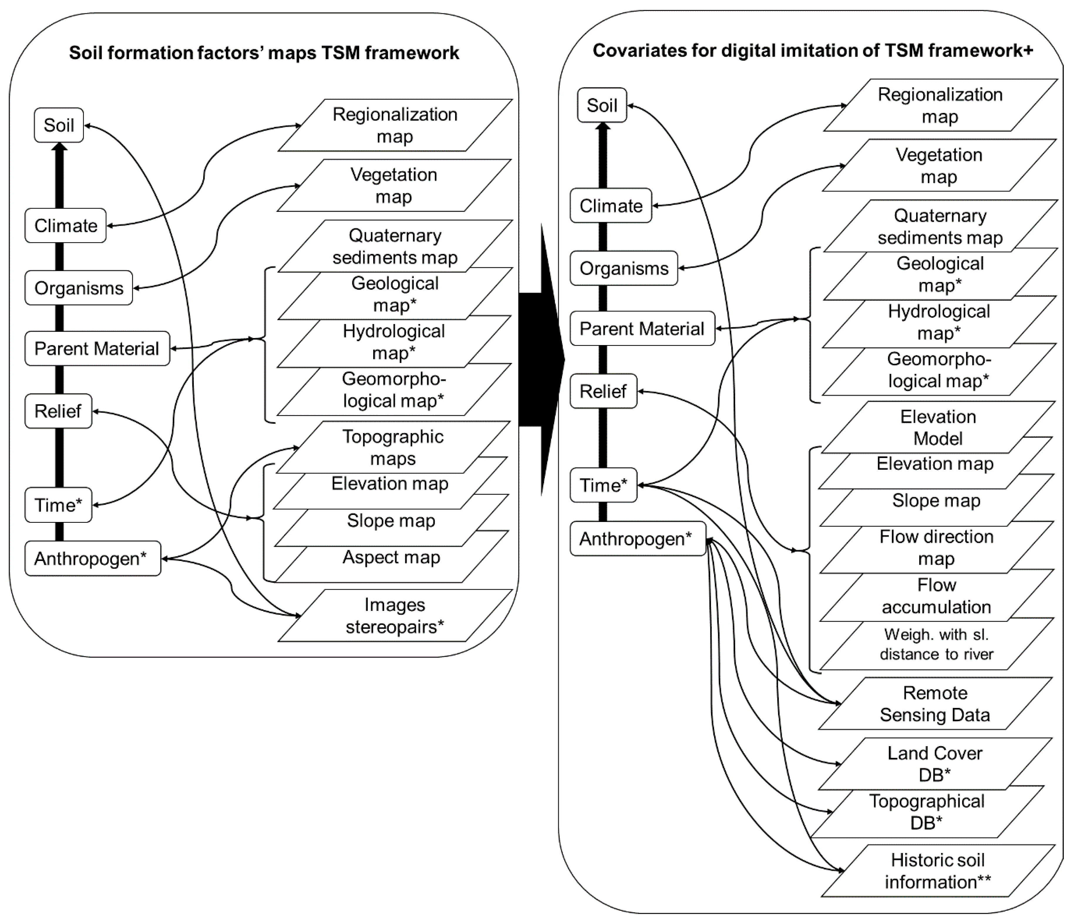
To develop the model, maps of the soil forming factors (covariates) that are the same as those used in traditional soil mapping (Figure 2) were added to the covariates. These covariates are based on the digital elevation model SRTM [43]—the distance to the nearest river weighted with the slopes and vertical terrain variation [25] and the flow accumulation index [44]. Using the weighted distance to the nearest river enabled us to imitate isoline (contour) frequency traditional expert analysis, and the distance to rivers from paper topographic maps was used to delineate the geomorphological units as river floodplains, river terraces and slopes, and watershed areas. In comparison to the widely used topography wetness index [45], the weighted distance is less dependent on noise in digital elevation models. Derivative maps that are based on the digital elevation model (slopes and flow directions) were calculated using the median filtered elevation model. A vegetation map was created using satellite image classification via the Random Forest method for a manually prepared learning sample set (Table 3). Overall, the producer and user accuracies of the vegetation class delineations exceeded 99.5%. The following covariates were prepared for modeling (Table 3).
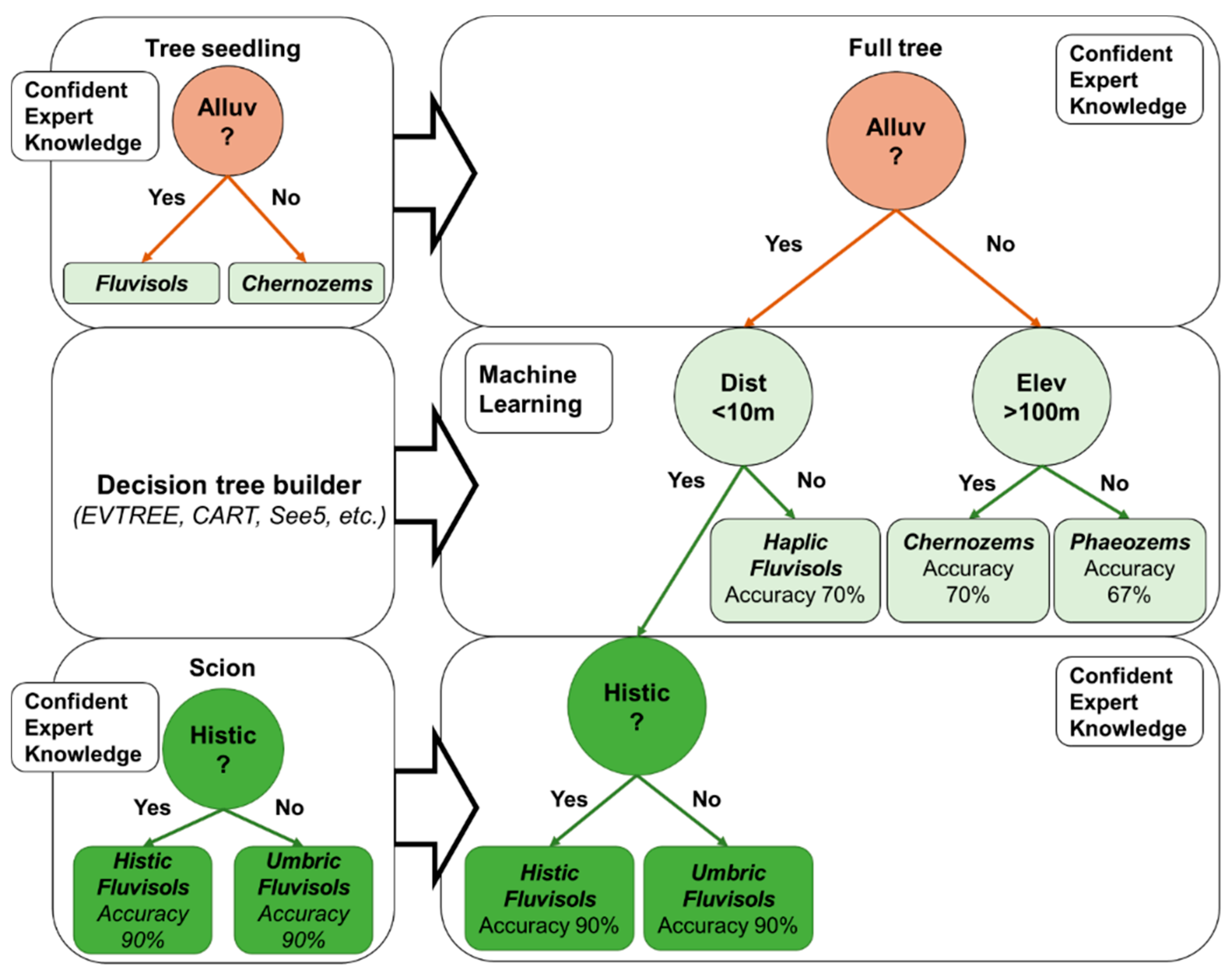
The proposed models for soil mapping were represented as decision trees. The main advantage of using decision trees is the possibility of intuitive manual correction. It is also possible to construct a seedling of a tree with branches that represent expert knowledge about soils (Figure 3). Such branches can be created to delineate large taxonomic groups of soils and specific soil properties. All unknown relationships can be extracted automatically via classification and regression tree algorithms, such as via the evolutionary learning of a globally optimal tree. The classification and regression tree algorithms should obtain an interpretable model. Consequently, this model needs to be compact and stable. After that, the full decision tree will contain all the required information for constructing the soil map (Figure 3). Such classification trees can be built for various soil regions and incorporated into a database to store the relevant knowledge of soils in a compact and explicit form. The obtained decision trees can also be linked to soil diagnostic features in soil classification systems to improve the soil classification systems or the decision trees themselves. Therefore, we considered two soil data sources: statistical knowledge in an interpretable form from decision trees extracted from legacy soil maps and expert knowledge from manual expert correction of the trees.
The implementation of the evolutionary learning of the globally optimal classification and regression tree algorithm from the EVTREE package in R was selected to construct the classification and regression trees [31]. The EVTREE algorithm aims at finding the optimal decision tree rather than one of the possible decision trees. This is important when trying to extract pedologically meaningful rules for soil mapping from legacy soil maps or the sample points obtained during soil surveys. This algorithm is based on concepts such as inheritance, mutation, and natural selection. These concepts are population-based, and a whole collection of candidate solutions—trees in this case—is processed simultaneously and iteratively modified by variation operators (namely, mutation (applied to single solutions) and crossover (merging multiple solutions) operators). Finally, a survivor selection process is used and favors solutions that perform well according to a specified quality criterion, which is usually called the evaluation function. In this evolutionary process, the mean quality of the population increases over time. A notable difference from comparable algorithms is the survivor selection mechanism here, with which it is essential to avoid premature convergence [31].
For most applications, globally optimal algorithms, in contrast to locally optimal algorithms, enable much more complete coverage of the parameter space, as follows:
where denotes the splitting variables, denotes the associated splitting rules for the internal nodes r, and M denotes the number of terminal nodes.
Equation (2) seeks trees that minimize the misclassification loss under a Bayesian information criterion (BIC) trade-off with the number of terminal nodes:
where loss(·,·) is a suitable loss function; X the predictor variable vector; Y is the response variable vector; comp(·) is a complexity function that is monotonically non-decreasing based on the number of terminal nodes M of the tree from ; and the overall parameter space is ; , the space of conceivable trees with M terminal nodes.
For EVTREE, the quality of a classification tree is most commonly measured as a function of its misclassification rate (MC) and the complexity of a tree is determined by a function of the number of terminal nodes M:
where N is the number of distinct values of predictor variables, comp describes the complexity function of a tree, and α is a user-specified parameter (default value α = 1). Notably, there are other possible rational values of α [15].
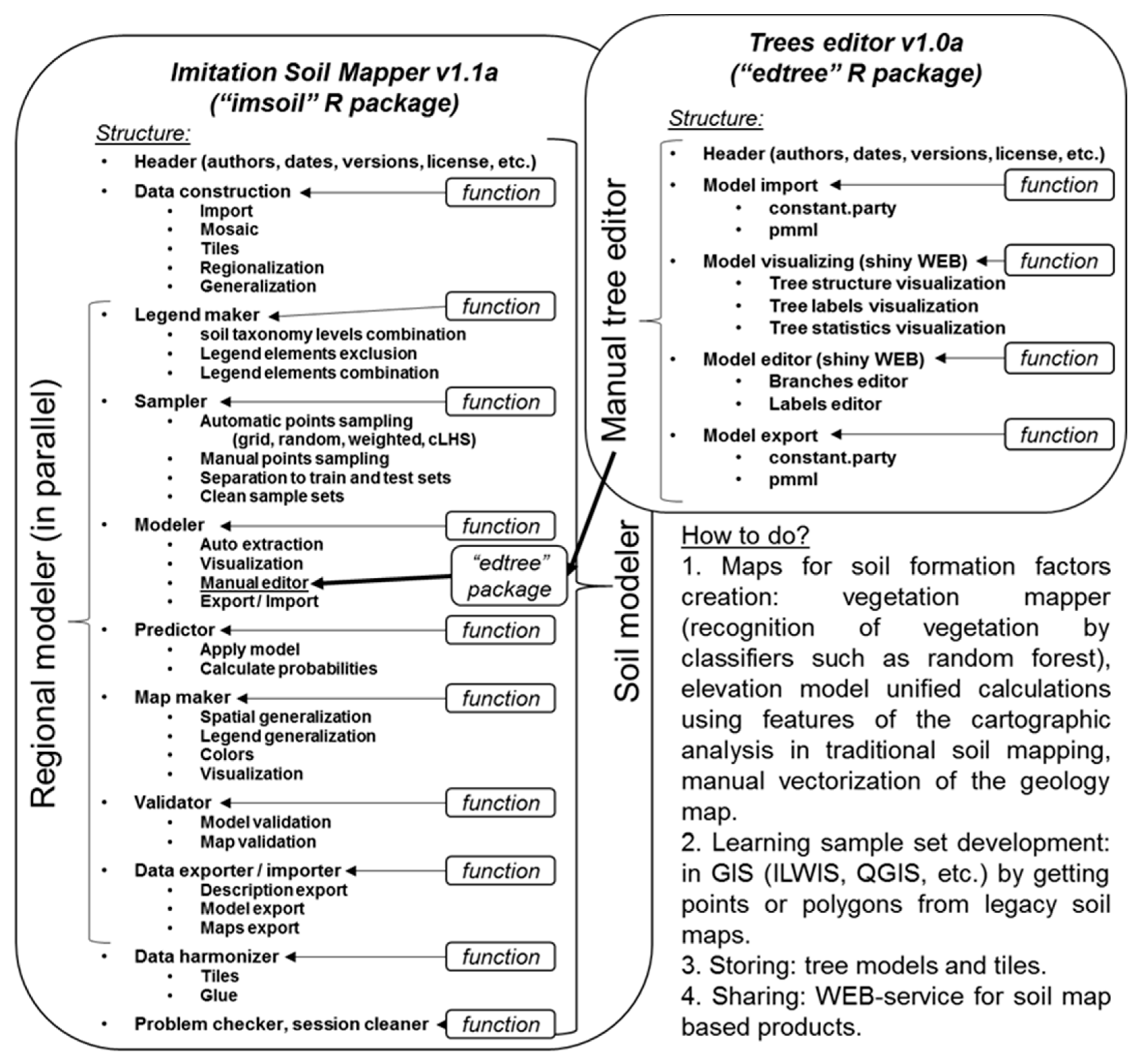
Using EVTREE as a method for finding the relationships between soil and soil formation factors, we implemented our approach of imitating the traditional soil mapping process in the R software packages (Figure 4). The main package, “imsoil”, was developed as a working experimental version. Development of the R package for the interactive manual correction of the “constparty” decision tree models from the “partykit” package was also required [46]. We used the model form “constparty” because it is widely used in various statistical packages and can be easily transformed into the classical format, “.pmml”.
To evaluate the real performance of EVTREE in the context of the proposed approach, the trees created by EVTREE were compared to trees created by the classic locally optimal algorithm, CART [47]. Currently, ensemble methods are the most common approaches for digital soil mapping due to their high predictive performance; hence, a comparison with Random Forest is also provided. Random Forest was selected as one of the best methods in terms of prediction accuracy [20].
The trees produced by CART were pruned to the smallest values of their complexity parameters (CPs). The number of minimum cases in the split for CART was equal to 10. The Gini splitting criterion was used for CART. For EVTREE modelling, we used the following parameters: minbucket = 10, minsplit = 20, niterations = 2000, ntrees = 50, alpha = 1, and maxdepth = 10. Prior probabilities for the branches of the CART and EVTREE decision trees were calculated via the 10-fold cross-validation procedure. Random Forest analysis with default settings from the randomForest package was then conducted.
The sample set we used consisted of 5001 points, as described above. Versions of the sample set with reduced numbers of sample points were also created to compare the performance of the methods for different sample set sizes.
The following criteria were used to assess the quality of soil–landscape relationship models:
- Stability: determined via an analysis of the dispersion of the number of branches and via expert analysis for 10 runs of an algorithm;
- Complexity: the number of conditions in the trees;
- Notional consistency: expert-based interpretation of one tree of each algorithm;
- The mean and minimum prior probabilities of proper classification were calculated as the mean and minimum number of properly classified points of a class from the training sample set in each tree terminal node divided by the total number of properly and improperly classified points in the same node;
- Spatial uncertainty in pixels: the mean probability of the most likely class for 10 runs of an algorithm;
- Map accuracy assessment: overall, the producer’s, user’s, and kappa accuracy [48]. The overall accuracy shows the number of similar depicted pixels in the predicted and reference maps multiplied by the total number of pixels. The producer’s accuracy represents the number of pixels that were depicted as part of the same class multiplied by the total number of that class’s pixels in the reference map. The user’s accuracy is the number of pixels that were depicted in the similar class but multiplied by the total number of that class’s pixels in the predicted map. The producer’s accuracy is associated with the error of misclassification, and the user’s accuracy is dedicated to the error of over-classification. The Cohen’s kappa index represents the overall accuracy considering the possibility of the agreement occurring by chance: , where po is the relative observed agreement among raters (identical to overall accuracy), and pe is the hypothetical probability of chance agreement, using the observed data to calculate the probabilities of each observer randomly seeing each category. For k categories, N observations to categorize and nki the number of times rater i predicted category k: .
The ten obtained decision trees were then expertly analyzed, and qualitative descriptions of the relationships between the soil and soil formation factors from the soil geography perspective were extracted from the trees. Then, qualitative decision trees were manually created, and statistical quantitative decision trees were packaged into them. This combination of qualitative descriptions and quantitative rules enabled further improvement of the prediction accuracy and the notional consistency of the soil mapping. This was accomplished by improving the list of covariates used for modelling and manually correcting the quantitative rules in accordance with qualitative information on the soil geography. Knowledge in the form of decision trees can be flexibly changed by the individual parameters and structures.
3. Results
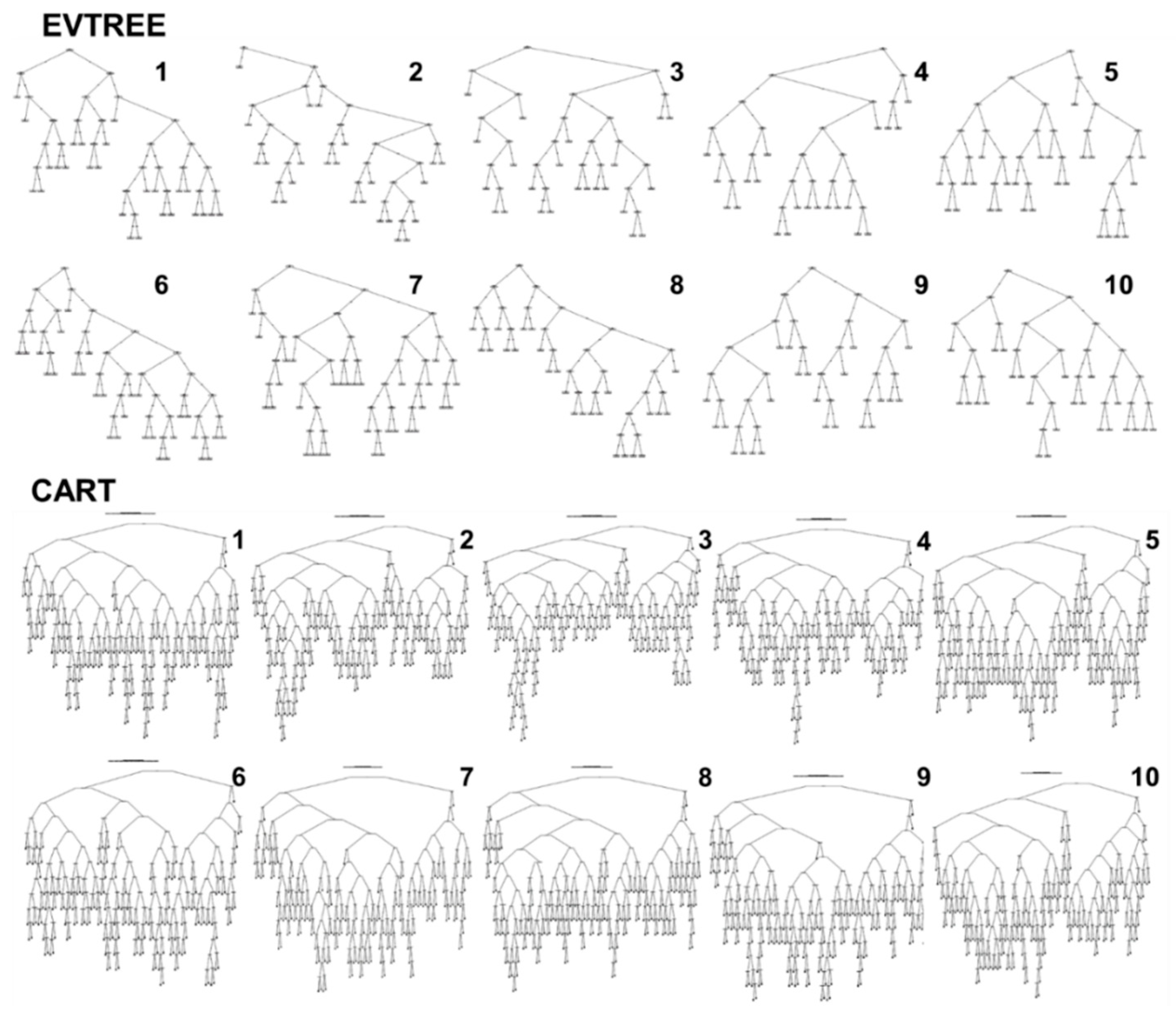
Decision trees with rules for soil delineation were created via the EVTREE and CART methods (Figure 5). All trees that were produced by EVTREE were of a similar size; the trees that were produced by CART were also of a similar size, and the trees that were produced by EVTREE were more compact than the CART trees. Moreover, the decision trees that were created by EVTREE had different sequences of similar rules for soil class delineation (Figure 5). All EVTREE trees, despite their formally different structures, presented similar relationships. The decision trees created by CART had similar rules for soil class delineation and similar sequences in the top part but different rules in the bottom part and, consequently, different sets of rules for soil class delineation.
The next example of rules for soil delineation is expressed in text form as follows:
3_G23—Grey and Dark Grey forest/Greyic Phaeozems Albic:
EVTREE_№5: (1) DEM_md15 < 203 m ^ RIVDIST >= 454505 m ^ DEM >= 171 m ^ LNDCVR = 45_Foret ^ DEM_md15 >= 203 m ^ 3_G23 (Probability: 12/15); (2) DEM_md15 >= 203 m ^ RIVDIST >= 333451 m ^ RIVDIST >= 371027 m ^ LNDCVR = 3_Water, 4_Leaf_Forest ^ 3_G23 (Probability: 47/58).
CART_№2: DEM < 171 m ^ RIVDIST < 337000 m ^ LNDCVR = 1_Grass, 2_Build_up_soils, 3_Water, 5_Coniferous_Forest ^ DEM_md15 < 203 m ^ (1) RIVDIST <= 539000 m ^ 3_G23 (Probability: 35/37); (2) DEM_ < 208 m ^ 3_G23 (Probability: 19/24); (3) DEM ->= 208 m ^ FLOWDIR = 2_E, 3_SE, 7_NW ^ 3_G23 (Probability: 4/10).
Description: EVTREE created branches for Phaeozem delineation in forests far from floodplains, where only leaf forests exist (Figure 6). CART created many branches with various elevation derivatives, including elevations, slopes, and flow directions. Hence, the rules for Phaeozem delineation were overlearned by CART.
Another example of the rules for soil delineation is expressed in text form as follows:
21_AL—Alluvial Meadow/Umbric Fluvisols Oxyaquic:
EVTREE_№5: DEM < 203 m ^ RIVDIST < 454,505 m ^ (1) LNDCVR = any except 2_Build-up_soils or 5_Coniferous_Forest ^ DEM_md15 < 160 m ^ RIVDIST < 23,679 m ^ 21_AL (Probability: 191/211); (2) LNDCVR = any except 2_Build-up_soils and 5_Coniferous_Forest ^ DEM_md15 >= 160 m ^ FLOWAC < 380 pixels ^ 21_AL (Probability: 33/64); (3) LNDCVR = 2_Build-up_soils or 5_Coniferous_Forest ^ ^ RIVDIST < 8398 m ^ 21_AL (Probability: 19/21).
CART_№2: DEM < 171 m ^ RIVDIST < 9305 m ^ 21_AL (Probability: 190/200); (2) DEM < 171 m ^ RIVDIST >= 9305 m ^ LNDCVR <> 1_Grass, 45_Mixed_Forest, 3_Water, 4_Leaf_Forest ^ FLOWAC >= 68 ^ FLOWDIR = 2_E, 8_N, 9_NE ^ DEM_md15 < 156 m ^ FLOWDIR = 2_E, 9_NE ^ RIVDIST < 212,000 m ^ DEM_md15 > 120 m ^ 21_AL (Probability: 3/10). Six other sets of rules for the delineation of Fluvisols (21_AL) were not included in the text because of their large size (more than eight branches). These sets were applied to the total number of 61 test points.
Description: EVTREE delineated most Fluvisols directly according to their elevations and distances to rivers weighted with slopes. These are the correct rules for Fluvisol delineation. The CART algorithm created many overlearned sets of rules that led to large areas of Fluvisols in the river terraces (Figure 6). Delineations by Random Forest were not correct as large areas of Fluvisols were identified in the river terraces instead of the floodplains (Figure 6). The rules for the delineation of Fluvisols obtained by EVTREE were much more direct than those obtained by CART.
The decision trees that were created using the evolutionary learning of globally optimal trees (EVTREE) had much higher notional consistency than the trees created using the classification and regression tree algorithm (CART).
The trees for the study area that were produced by EVTREE had 20–29 conditions in comparison to 142–162 conditions for the trees that were produced by CART (Table 4). The mean and minimum prior probabilities were similar for both methods (Table 4). The minimum prior probabilities were related to typical Chernozem soil in both the EVTREE and CART methods. Thus, the EVTREE models are much more compact, which facilitates their interpretation.
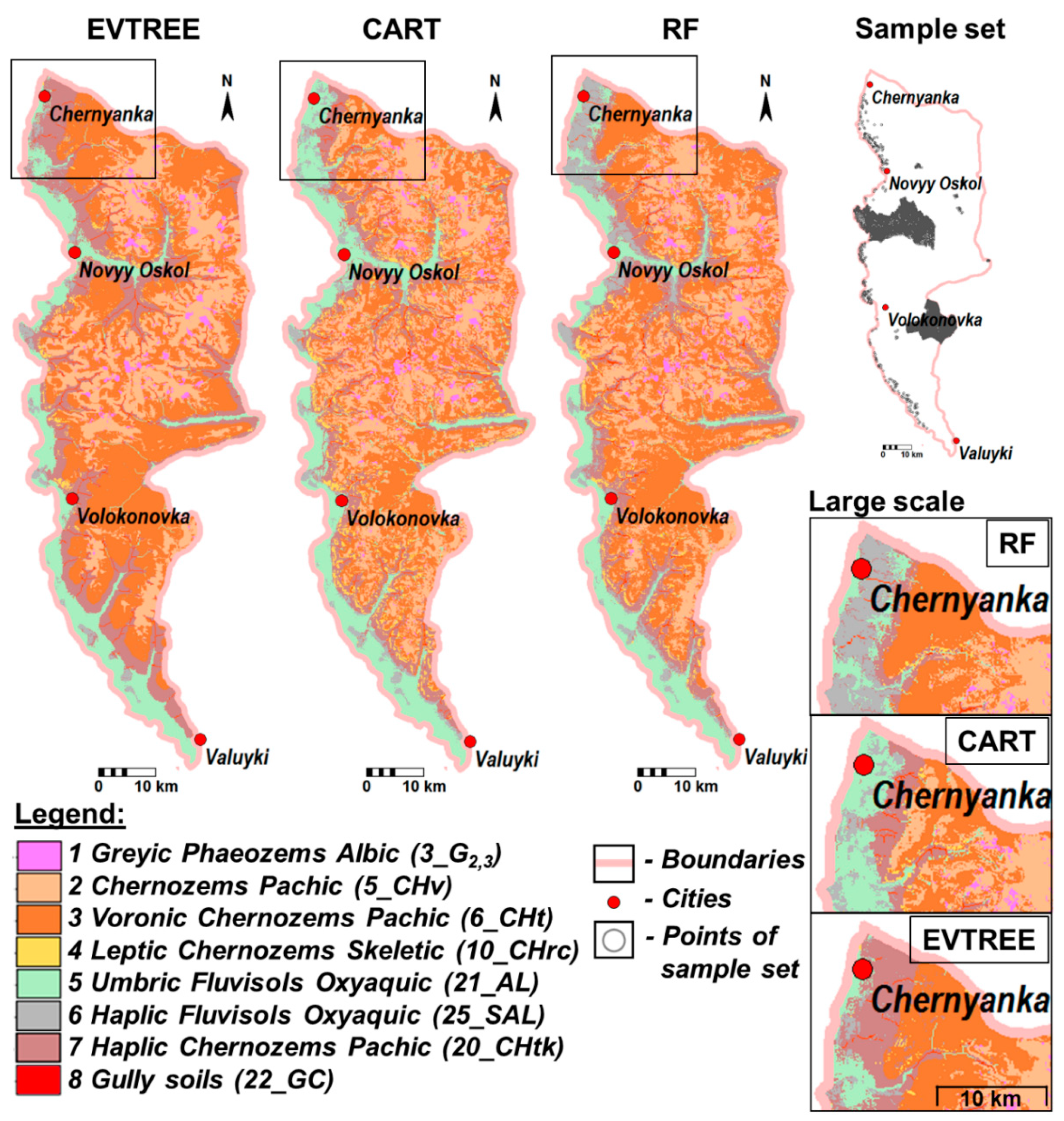
The soil maps were generally similar but exhibited some local differences (Figure 7). Fluvisols were correctly mapped using only EVTREE as they were always associated with the rivers’ floodplains and not the rivers’ terraces or watershed areas. EVTREE selected the simplest rules for Fluvisols that gave the best accuracy. For soils with complex soil–landscape relationships, EVTREE offers less accuracy than CART. However, its method of selecting the simplest rules is much closer to the traditional approach.
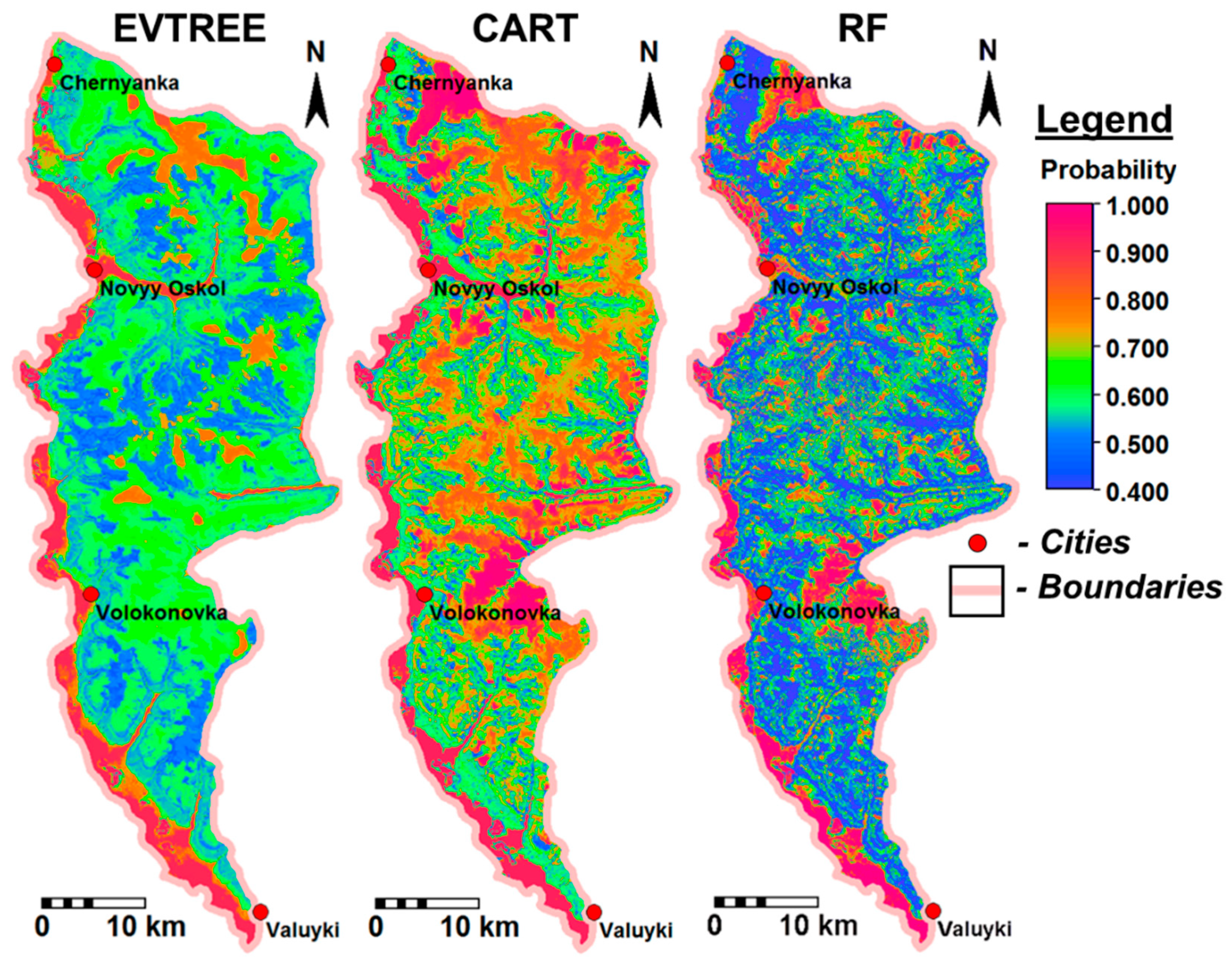
The overall accuracy of the soil map created via Random Forest using the full sample set was 87% (Table 5). Possibly, a part of the remaining 13% could be mapped using information about previous soil formation factors (soil formation factors such as the vegetation and climate that existed a thousand years ago could substantially affect the properties of soils but are not currently represented by covariates in digital soil mapping). The probability map created via the Random Forest algorithm demonstrated moderate quality, as the mean probability was 0.60 (Figure 8). Despite the moderate quality of the model, Random Forest correctly predicted 87% of the independent test sample set. The CART probability map showed a high mean probability of more than 80% for large areas, while the real prediction accuracy was only 67%. As in other studies, the Random Forest model demonstrated the best prediction accuracy for the full sample set [20].
The EVTREE probability map yielded moderate and high accuracy for watershed areas and floodplains, where the delineation of soils was easier. The lowest probabilities for EVTREE were observed for watershed slopes, where the delineation of Chernozem soils was not clear. For the Random Forest approach, the low accuracy on the probability map corresponded to occasionally satisfactory prediction accuracy, as measured by the test set, despite using many test points (approximately 2000 points). Therefore, only the probability map created by EVTREE was adequate. Notably, the limited number of covariates provided an advantage to EVTREE, while the approach using stochastic calculation of the probability map was not optimal.
After reducing the size of the training sample set from 5001 to 3304 points by reducing the squared areas with sample points (2 km2), the accuracy remained the same for the CART and EVTREE methods, but for Random Forest, the accuracy decreased substantially by 20–30% (Table 6). After increasing the mean distance between points by reducing the number of points from 5001 to 1785, the accuracy of all three methods decreased proportionally. When increasing the mean distance between points by reducing the size of the sample set to 1000 points, the Random Forest algorithm failed to run, and EVTREE and CART yielded similar accuracy to that used for 1785 points. For the small sample set, EVTREE and CART have an advantage over Random Forest because they can deal with a small number of cases.
The decision trees obtained with the quantitative cartographic rules of soil unit delineation were analyzed to extract the real geographical qualitative relationships between the soil and soil formation factors, like those that were formulated via traditional soil mapping (Figure 9).
The obtained qualitative decision tree was represented in the form of separate rule chains for each soil. The rule chains were also split into environmental niches (Figure 10).
Analysis of the soil delineation showed that Fluvisols (21_AL) and Gully complexes (22_GC) were not correctly mapped. This occurred because of the overly simplified river map, which led to a rough river distance map. The quality of the soil predictions can be improved by corrections of the soil formation factors maps. Consequently, we decided to rebuild the river distance map. We rebuilt the river and river distance maps using a parameter of river length equal to 100 m instead of 1000 m. This parameter represented the minimal length of a river on the map. Then we reran the EVTREE algorithm with the new input river distance map. In the resulting soil map, the visual difference between Fluvisols (21_AL) and the Gully complex (22_GC) soils was excellent. In the rebuilt tree, information about Chernozems calcareous soils (10_CHrc) was added. On the large-scale soil maps, these soils were mapped in the areas of outcrops. Such areas were recognized using Landsat satellite images and the supervised classification algorithm with the maximum likelihood method. For teaching, the original soil sample set for only outcrop areas was used. Then, the rule for accurately delineating Chernozems calcareous (10_CHrc) soils in the areas of the outcrops was added to the classification tree (Figure 11).
Therefore, there were at least four ways to correct the soil map:
- The addition of more accurate covariate maps to the analysis;
- manual tree correction;
- change in qualitative rules;
- change in quantitative rules;
- manual soil map unit correction.
An accuracy assessment was provided for the corrected soil map using another independent sample set of 1269 soil pits. The overall accuracy before manual correction was 65%, with 76% accuracy after correction. Therefore, based on soil geography knowledge, the covariates for the modelling and quantitative models were corrected by an expert to provide higher accuracy and notional consistency of the soil maps.
4. Discussion
We obtained accurate soil maps automatically and made them much more accurate manually. The accuracy of the manually corrected soil map can reach one hundred percent, but this requires laborious work. The developed framework allowed us to implement the work of a traditional soil-mapper using the statistical method of evolutionary trees and the understandable representation of soil mapping rules. This statistical method was first used for digital soil mapping. The advantages of this method over the CART method are the compactness and reasonability of the model. The easy-to-use representation of soil–landscape relationships—as a decision tree and chains of rules—is an advantage of the proposed approach compared to structural equation modelling [12,21]. However, for mapping continuous soil properties, these two approaches can be used together. This process involves mapping soil units with classification trees and then splitting them into continuous soil property maps (Figure 12).
This framework differs from the SoLIM because it aims at the development of approaches that fully imitate the work of a traditional soil mapper. Thus, the representation of the classification trees and rule chains was closely investigated. In our methodology, we used mostly traditional soil formation factor maps, such as geological parent materials and simple derivatives of the digital elevation model, rather than difficult indexes. We also used a traditional representative form of soil units instead of a fuzzy logic approach. Our framework and the package we developed provide a traditional soil mapping alternative to SoLIM [22,23]. Realization of this framework was strongly based on machine learning techniques and the advantages of the R statistical language, which make it congruent with the SoilGRIDs framework [7].
The proposed forms of the relationships between the soil and soil formation factors, classification trees, and rule chains appear to be very convenient for interpretation. Qualitatively describing the quantitative rules was also simple, despite some subjective factors due to the expert nature of the analysis. Using mostly traditional soil formation factor maps helped us interpret the quantitative model and easily obtain the qualitative model. The obtained qualitative classification tree allowed us to visualize the complex environmental relationships for the study area in a form that is understandable for traditional natural scientists, soil scientists, geologists, ecologists, environmentalists, and others. This form is useful for environmental analysis, such as determining the reasons to change soils over time and defining the environmental state of the study area. This is a traditional type of analysis that is neglected in most other DSM methodologies. The soil mapping chains of the rule form were convenient for making the soil map and were manually corrected. This simple form can be programmed to make soil maps in most GIS programs. The novelty (associated with the chains of the rules) of our methodology compared to SoLIM is that our method uses groups based on environmental niches that are important for investigating the underlying reasons for soil geography. A considerable problem with our framework is the laborious work associated with the process of translating the relationships from the form of classification trees to rule chains. This process, however, can be automated and allowed us to collect important expert soil geography information.
Below we summarize the problems that we aimed to solve with the proposed framework.
- The laborious manual work associated with producing two forms of soil rules as a general classification tree and soil-specific rule chains. A possible solution is using a package with an interface that allows one to make adjustments as easily as possible. Moreover, this method should permit automatic transformations between classification trees and chains of rules.
- The significant changes in the classification trees when using updated covariate maps. This can be overcome by using more sophisticated statistical methods of finding classification rules and incorporating prior soil knowledge into the search for rules.
- The mapping of soil classes when we need to map continuous soil properties or soil functions. Compliance with other methodologies provides a solution for this problem. In that case, the proposed framework offers an interface with legacy soil maps.
- Statistical improvements of the classification tree algorithm’s accuracy.
5. Conclusions
- The overall accuracy of the soil maps in the study area was 59%, 67%, and 87% for EVTREE, CART, and Random Forest, respectively. The prediction accuracy of EVTREE for the study area was slightly lower than that for CART and substantially lower than that for Random Forest. After reducing the size of the sample set from 5001 to 1785 points, the accuracy remained the same for EVTREE (59%), decreased for CART (61%), and decreased substantially for Random Forest (62%). With a sample set of 1000 points, the Random Forest algorithm failed to run, and EVTREE and CART realized similar accuracy to 1785 points. The reduced sample sets covered all soils and most soil formation factor features of the original entire sample set. Therefore, the quality of soil classification under EVTREE was much less dependent on the size of the sample set.
- The mean size of the trees in the study area constructed by EVTREE included 24 conditions, compared to the 154 conditions for the trees constructed by CART. The compact decision trees that were constructed by EVTREE were convenient for both quantitative quality assessment and expert-based notional tracing.
- The soil maps that were created using EVTREE had much higher notional consistency than the maps created using CART. The rules formulated by EVTREE for the delineation of Fluvisols and Phaeozems were much more direct than those formulated by CART. The direct models constructed by EVTREE for soil mapping are suitable for full or partial extrapolation to distant territories in the world with similar environmental conditions.
- The R package is required for the manual “constparty” decision tree model corrections, which can correct conditions and labels. The features for selecting tree branches and linking the tree with the associated soil map for the online monitoring of changes will be useful.
- We developed a digital soil mapping framework that imitates the process of traditional soil mapping and incorporates qualitative knowledge about soil geography into the quantitative rules for soil delineation. This model in the form of a decision tree can be expertly analyzed, and improvements can be made to the covariate list and notional consistency of the model.
- Challenges include the development of an easy-to-use and fast visual tree editor, automatic transformation of the classification trees to soil-specific rule chains, automatic statistical incorporation of prior soil knowledge in the process of tree building, and compliance with other methods for mapping continuous soil properties and soil functions.
Author Contributions
Conceptualization, Igor Savin; methodology, Arseniy Zhogolev and Igor Savin; software, Arseniy Zhogolev; validation, Arseniy Zhogolev; formal analysis, Arseniy Zhogolev; investigation, Arseniy Zhogolev; resources, Arseniy Zhogolev and Igor Savin; data curation, Arseniy Zhogolev and Igor Savin; writing—original draft preparation, Arseniy Zhogolev and Igor Savin; writing—review and editing, Igor Savin; visualization, Arseniy Zhogolev; funding acquisition, Igor Savin. All authors have read and agreed to the published version of the manuscript.
Funding
This research was funded bythe support of the “RUDN University Program 5-100” and the RFBR grant N 19-05-50063, as well as by the support of the Ministry of Science and Higher Education of Russian Federation (Agreement No. 075-15-2020-805).
Acknowledgments
We thank Praskovya Grubina for help with preparing the sample set for modelling.
Conflicts of Interest
The authors declare no conflict of interest. The funders had no role in the design of the study; in the collection, analyses, or interpretation of data; in the writing of the manuscript, or in the decision to publish the results.
References
- Arrouays, D.; McBratney, A.B.; Minasny, B.; Hempel, J.W.; Heuvelink, G.B.M.; MacMillan, R.A.; McKenzie, N.J. The GlobalSoilMap Project Specifications. In GlobalSoilMap: Basis of the Global Spatial Soil Information System; CRC Press: Boca Raton, FL, USA, 2014. [Google Scholar]
- Arrouays, D.; Richer-de-Forges, A.C.; McBratney, A.B.; Hartemink, A.E.; Minasny, B.; Savin, I.; Lagacherie, P. The GlobalSoilMap project: Past, present, future, and national examples from France. Dokuchaev Soil Bull. 2018, 95, 3–23. [Google Scholar] [CrossRef]
- Arrouays, D.; Savin, I.; Leenaars, J.; McBratney, A.B. (Eds.) GlobalSoilMap—Digital Soil Mapping from Country to Globe; CRC Press: London, UK, 2017. [Google Scholar]
- Lagacherie, P.; McBratney, A.B. Chapter 1. Spatial soil information systems and spatial soil inference systems: Perspectives for digital soil mapping: Review article. Digital Soil Mapping. An introductory perspective. Dev. Soil Sci. 2007, 31, 137–150. [Google Scholar]
- Arrouays, D.; Leenaars, J.G.; Richer-de-Forges, A.C.; Adhikari, K.; Ballabio, C.; Greve, M.; Heuvelink, G. Soil legacy data rescue via GlobalSoilMap and other international and national initiatives. GeoResJ 2017, 14, 1–19. [Google Scholar] [CrossRef]
- Grunwald, S.; Thompson, J.A.; Boettinger, J.L. Digital soil mapping and modeling at continental scales: Finding solutions for global issues. Soil Sci. Soc. Am. J. 2011, 75, 1201–1213. [Google Scholar] [CrossRef]
- Hengl, T.; de Jesus, J.M.; Heuvelink, G.B.; Gonzalez, M.R.; Kilibarda, M.; Blagotić, A.; Guevara, M.A. SoilGrids250m: Global gridded soil information based on machine learning. PLoS ONE 2017, 12, e0169748. [Google Scholar] [CrossRef] [Green Version]
- Lagacherie, P. Digital soil mapping: To state-of-the-art. In Digital Soil Mapping with Limited Data; Springer: Dordrecht, The Netherlands, 2008; pp. 3–14. [Google Scholar]
- McBratney, A.B.; de Gruijter, J.; Bryce, A. Pedometrics Timeline. Geoderma 2019, 338, 568–575. [Google Scholar] [CrossRef]
- Mulder, V.L.; De Bruin, S.; Schaepman, M.E.; Mayr, T.R. The use of remote sensing in soil and terrain mapping—A review. Geoderma 2011, 162, 1–19. [Google Scholar] [CrossRef]
- Qi, F.; Zhu, A.X. Knowledge discovery from soil maps using inductive learning. Int. J. Geogr. Inf. Sci. 2003, 17, 771–795. [Google Scholar] [CrossRef]
- Angelini, M.E.; Heuvelink, G.B.M.; Kempen, B.; Morrás, H.J.M. Mapping the soils of an Argentine Pampas region using structural equation modeling. Geoderma 2016, 281, 102–118. [Google Scholar] [CrossRef]
- Bui, E.N.; Henderson, B.L.; Viergever, K. Knowledge discovery from models of soil properties developed through data mining. Ecol. Modeling 2006, 191, 431–446. [Google Scholar] [CrossRef]
- McBratney, A.B.; Santos, M.M.; Minasny, B. On digital soil mapping. Geoderma 2003, 117, 3–52. [Google Scholar] [CrossRef]
- Zhogolev, A.V. A comparison of SoilGRIDs with the Disaggregated State Soil Map of Russia. In GlobalSoilMap—Digital Soil Mapping from Country to Globe; CRC press: London, UK, 2017; pp. 49–52. [Google Scholar]
- Odgers, N.P.; Sun, W.; McBratney, A.B.; Minasny, B.; Clifford, D. Disaggregating and harmonising soil map units through resampled classification trees. Geoderma 2014, 214, 91–100. [Google Scholar] [CrossRef]
- Pásztor, L.; Laborczi, A.; Takács, K.; Szatmári, G.; Bakacsi, Z.; Szabó, J. DOSoReMI as the National Implementation of GlobalSoilMap for the Territory of Hungary. In GlobalSoilMap—Digital Soil Mapping from Country to Globe; CRC Press: London, UK, 2017; pp. 17–22. [Google Scholar]
- Caubet, M.; Dobarco, M.R.; Arrouays, D.; Minasny, B.; Saby, N.P.A. Merging country, continental and global predictions of soil texture: Lessons from ensemble modeling in France. Geoderma 2019, 337, 99–110. [Google Scholar] [CrossRef]
- Chinilin, A.V.; Savin, I.Y. The large-scale digital mapping of soil organic carbon using machine learning algorithms. Dokuchaev Soil Bull. 2018, 91, 46–62. [Google Scholar] [CrossRef]
- Hengl, T.; Nussbaum, M.; Wright, M.N.; Heuvelink, G.B.M.; Gräler, B. Random Forest as a generic framework for predictive modelling of spatial and spatio-temporal variables. PeerJ 2018, 6, e5518. [Google Scholar] [CrossRef] [PubMed] [Green Version]
- Angelini, M.E.; Heuvelink, G.B.M.; Kempen, B. Multivariate mapping of soil with structural equation modeling. Eur. J. Soil Sci. 2017, 68, 575–591. [Google Scholar] [CrossRef] [Green Version]
- Zhu, A.; Cheng-Zhi, Q.; Peng, L.; Fei, D. Digital soil mapping for smart agriculture: The SoLIM method and software platforms. Rudn J. Agron. Anim. Ind. 2018, 13, 317–335. [Google Scholar] [CrossRef]
- Zhu, A.X.; Band, L.E.; Dutton, B.; Nimlos, T.J. Automated soil inference under fuzzy logic. Ecol. Modeling 1996, 90, 123–145. [Google Scholar] [CrossRef]
- Qi, F.; Zhu, A.X. Comparing three methods for modeling the uncertainty in knowledge discovery from area-class soil maps. Comput. Geosci. 2011, 37, 1425–1436. [Google Scholar] [CrossRef]
- Zhogolev, A.V.; Savin, I.Y. Automated updating of medium-scale soil maps. Eurasian Soil Sci. 2016, 49, 1241–1249. [Google Scholar] [CrossRef]
- Bui, E.N. Data-driven Critical Zone science: A new paradigm. Sci. Total Environ. 2016, 568, 587–593. [Google Scholar] [CrossRef] [PubMed]
- Ma, Y.X.; Minasny, B.; Malone, B.P.; McBratney, A.B. Pedology and Digital Soil Mapping (DSM). Eur. J. Soil Sci. 2019, 70, 216–235. [Google Scholar] [CrossRef]
- Padarian, J.; Morris, J.; Minasny, B.; McBratney, A.B. Pedotransfer Functions and Soil Inference Systems; Springer: Berlin/Heidelberg, Germany, 2018; pp. 195–220. [Google Scholar]
- Lagacherie, P. Formalisation des Lois de Distribution des Sols Pour Automatiser la Cartographie Pédologique à Partir d’un Secteur Pris Comme Reference. Master’s Thesis, Université de Montpellier, Institut National de la Recherche Agronomique, Montpellier, France, 1992. [Google Scholar]
- Therneau, T.M.; Atkinson, E.J. An Introduction to Recursive Partitioning Using the RPART Routines. 2018. Available online: https://cran.r-project.org/web/packages/rpart/vignettes/longintro.pdf (accessed on 28 February 2019).
- Grubinger, T.; Zeileis, A.; Pfeiffer, K.P. Evtree: Evolutionary Learning of Globally Optimal Classification and Regression Trees in R. J. Stat. Softw. 2014, 61, 1–29. [Google Scholar] [CrossRef] [Green Version]
- Balestriero, R.; Baraniuk, R. A spline theory of deep learning. In Proceedings of the 35th International Conference on Machine Learning, Stockholm, Sweden, 10–15 July 2018; Volume 80, pp. 374–383. [Google Scholar]
- Chimatapu, R.; Hagras, H.; Starkey, A.; Owusu, G. Explainable AI and Fuzzy Logic Systems. In International Conference on Theory and Practice of Natural Computing; Springer: Berlin/Heidelberg, Germany, 2018; pp. 3–20. [Google Scholar]
- Savin, I.Y. Computer-Based Imitation of Soil Mapping. Digital Soil Mapping: Theoretical and Experimental Investigations; V.V. Dokuchaev Soil Science Institute: Moscow, Russia, 2012; pp. 26–34. (In Russian) [Google Scholar]
- Egorov, V.V.; Fridland, V.M.; Ivanova, E.N.; Rozov, N.N. Classification and Diagnostics of Soils of the Soviet Union; Kolos: Moscow, Russia, 1977. (In Russian) [Google Scholar]
- Shishov, L.L.; Tonkonogov, V.D.; Lebedeva, I.I.; Gerasimova, V.I. (Eds.) Classification and Diagnostic System of Russian Soils; Oikumena: Smolensk, Russia, 2004. (In Russian) [Google Scholar]
- IUSS Working Group WRB. World Reference Base for Soil Resources 2006; World Soil Resources Reports 103; FAO: Rome, Italy, 2006. [Google Scholar]
- Ilyina, L.P.; Mihailova, R.P.; Simakova, M.S.; Shubina, I.G. Compilation of the Regional Medium-Scale Soil Maps with Representation of Patterns of Soil Cover; V.V. Dokuchaev Soil Science Institute: Moscow, Russia, 1990. [Google Scholar]
- Soil Survey Staff. Soil Taxonomy: A Basic System of Soil Classification for Making and Interpreting Soil Surveys, 2nd ed.; Agriculture Handbook, 436; Natural Resources Conservation Service: Washington, DC, USA; U.S. Department of Agriculture: Washington, DC, USA, 1999.
- Zinck, J.A. Physiography and Soils. In Soil Survey Courses. International Institute for Aerospace and Earth Sciences; ITC: Enschede, The Netherlands, 1988. [Google Scholar]
- Hengl, T. Finding the right pixel size. Comput. Geosci. 2006, 32, 1283–1298. [Google Scholar] [CrossRef]
- Xiong, L.Y.; Zhu, A.X.; Zhang, L.; Tang, G.A. Drainage basin object-based method for regional-scale landform classification: A case study of loess area in China. Phys. Geogr. 2018, 39, 523–541. [Google Scholar] [CrossRef]
- Jarvis, A.; Reuter, H.I.; Nelson, A.; Guevara, E. Hole-filled SRTM for the Globe Version 4. Available online: http://srtm.csi.cgiar.org (accessed on 28 February 2019).
- Qin, C.Z.; Zhu, A.X.; Pei, T.; Li, B.L.; Scholten, T.; Behrens, T.; Zhou, C.H. An approach to computing topographic wetness index based on maximum downslope gradient. Precis. Agric. 2011, 12, 32–43. [Google Scholar] [CrossRef]
- Hengl, T.; Maathuis, B.H.P.; Wang, L. Geomorphometry in ILWIS. Dev. Soil Sci. 2009, 33, 309–331. [Google Scholar]
- Hothorn, T.; Zeileis, A. Partykit: A modular toolkit for recursive partytioning in R. J. Mach. Learn. Res. 2015, 16, 3905–3909. [Google Scholar]
- Breiman, L.; Friedman, J.; Olshen, R.; Stone, C. Classification and regression trees. Wadsworth Int. Group 1984, 37, 237–251. [Google Scholar]
- Rossiter, D.G.; Zeng, R.; Zhang, G.L. Accounting for taxonomic distance in accuracy assessment of soil class predictions. Geoderma 2017, 292, 118–127. [Google Scholar] [CrossRef] [Green Version]
Figure 1.
Study area Novy Oskol.

Figure 2.
Covariates from the traditional methodology of soil mapping with additional maps of the elevation model derivatives (*—optionally used maps and **—historical information about soils that are required for correct monosemantic soil delineation via the soil formation factor approach).
Figure 2.
Covariates from the traditional methodology of soil mapping with additional maps of the elevation model derivatives (*—optionally used maps and **—historical information about soils that are required for correct monosemantic soil delineation via the soil formation factor approach).

Figure 3.
Completing a decision tree of confident expert knowledge with additional branches via machine learning (evtree package). Dist—distance to the nearest river weighted by slopes, Elev—elevation, Alluv—alluvial deposits in floodplains, and Histic—appearance of the Histic soil horizon with organic material (Accuracy: 90% refers to the accuracy of recognizing the soil organic surfaces based on Landsat satellite images).

Figure 4.
Structure of our ongoing R packages with implementation of the traditional soil mapping imitation approach.
Figure 4.
Structure of our ongoing R packages with implementation of the traditional soil mapping imitation approach.

Figure 5.
The appearance of the trees that were created via EVTREE and CART.

Figure 6.
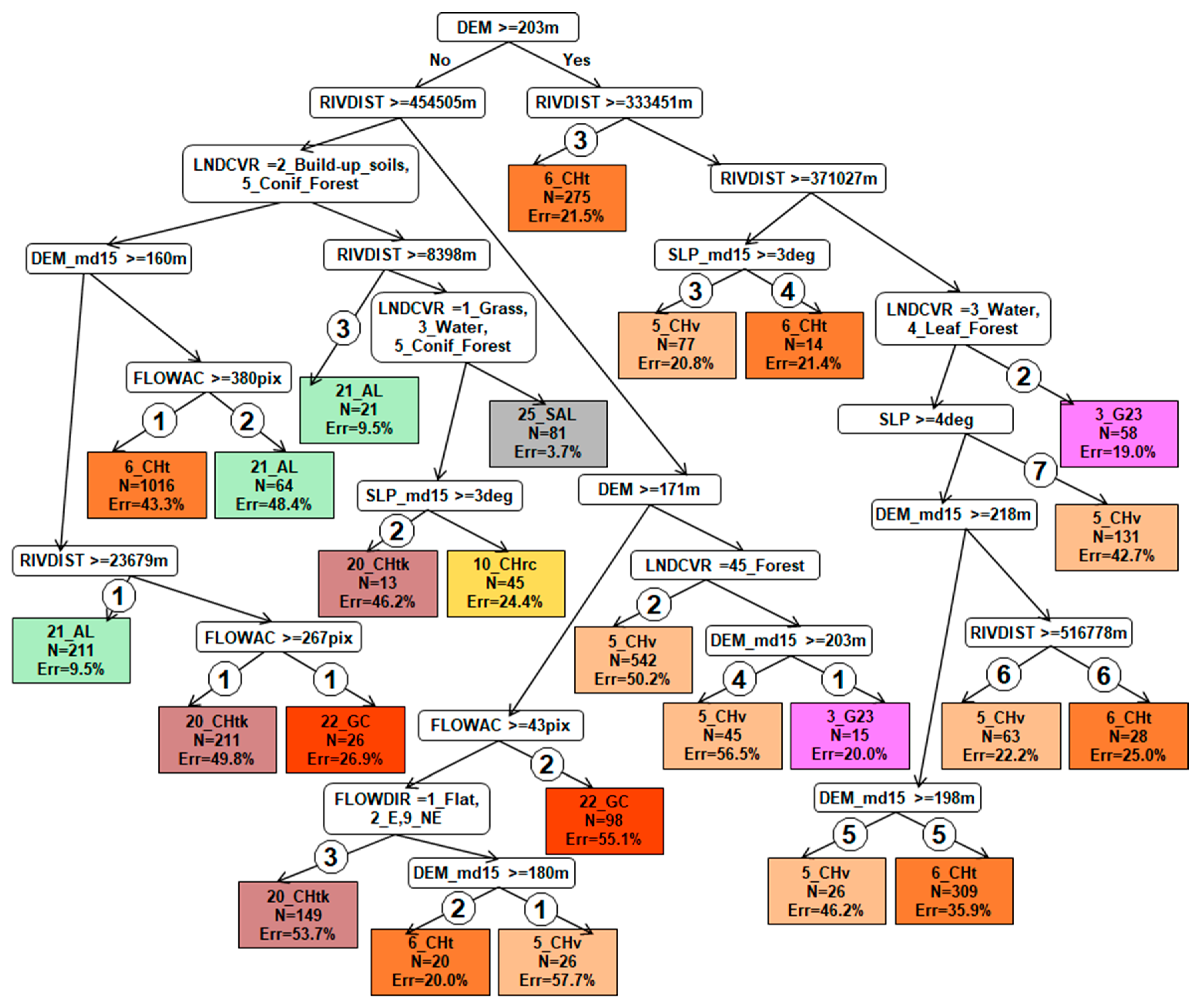
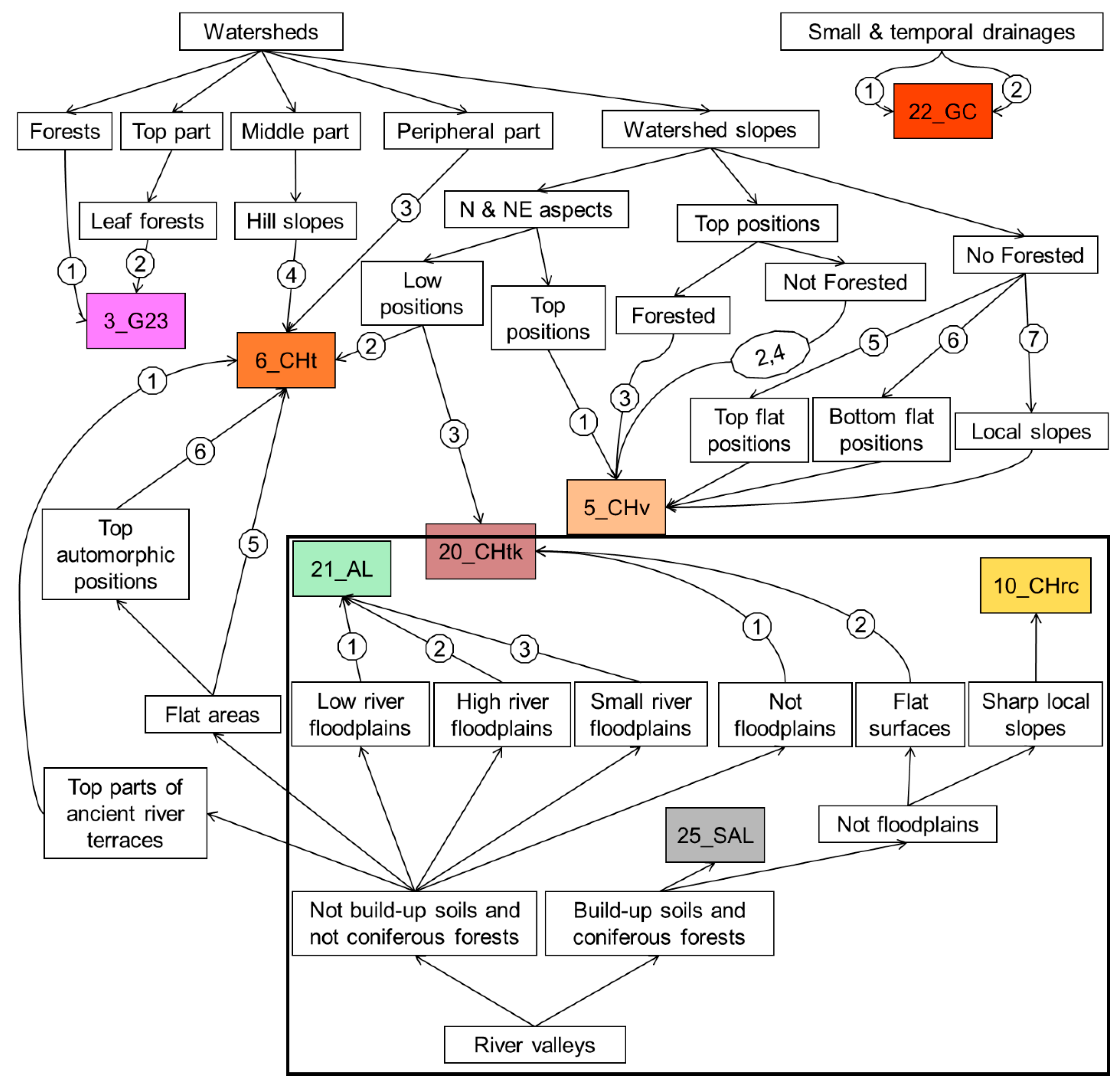
EVTREE quantitative decision tree №5 for the Chernozems soil zone in the Belgorod region (Soil Types: 3_G23—Greyic Phaeozems Albic, 5_CHv—Voronic Chernozems Pachic, 6_CHt—Voronic Chernozems Pachic, 10_CHrc—Leptic Chernozems, 20_CHtk—Leptic Voronic Chernozems Pachic, 21_AL—Umbric Fluvisols Oxyaquic, 22_GC—Gully Complex, 25_SAL—Haplic Fluvisols, N: number of the points with the soil, Err: misclassification rate).
Figure 6.
EVTREE quantitative decision tree №5 for the Chernozems soil zone in the Belgorod region (Soil Types: 3_G23—Greyic Phaeozems Albic, 5_CHv—Voronic Chernozems Pachic, 6_CHt—Voronic Chernozems Pachic, 10_CHrc—Leptic Chernozems, 20_CHtk—Leptic Voronic Chernozems Pachic, 21_AL—Umbric Fluvisols Oxyaquic, 22_GC—Gully Complex, 25_SAL—Haplic Fluvisols, N: number of the points with the soil, Err: misclassification rate).

Figure 7.
Sample set and soil maps that were created using the three methods: EVTREE, CART, and Random Forest.
Figure 7.
Sample set and soil maps that were created using the three methods: EVTREE, CART, and Random Forest.

Figure 8.
Probability maps of the most likely soil class created using three methods: EVTREE (stochastic), CART (stochastic), and Random Forest.
Figure 8.
Probability maps of the most likely soil class created using three methods: EVTREE (stochastic), CART (stochastic), and Random Forest.

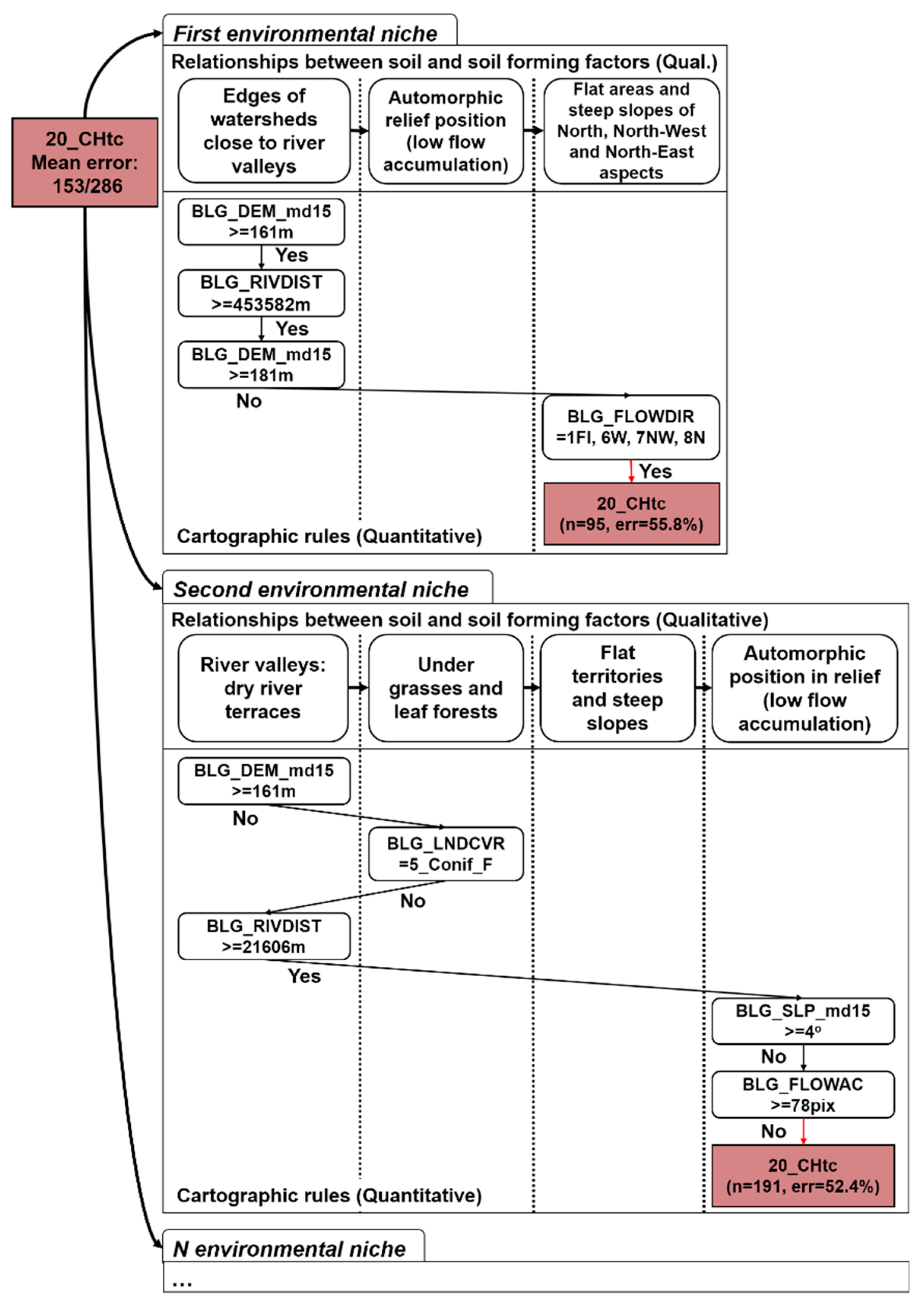
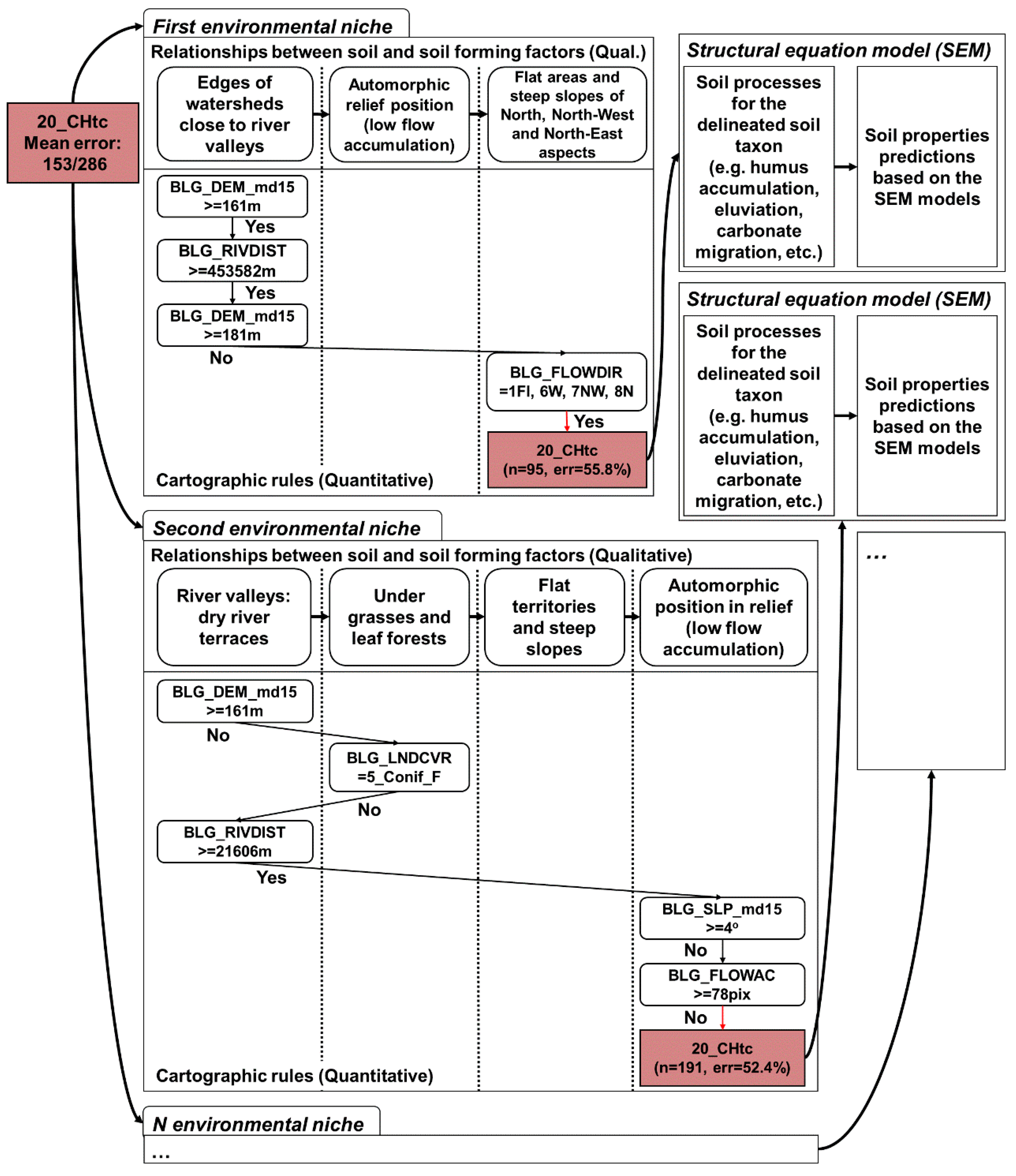
Figure 9.
The qualitative decision tree with the numbers of rules from the quantitative decision tree (in the square—the part of the tree that was expertly corrected).
Figure 9.
The qualitative decision tree with the numbers of rules from the quantitative decision tree (in the square—the part of the tree that was expertly corrected).

Figure 10.
Packaging of the quantitative cartographic rules of soil unit delineation with qualitative rules.
Figure 10.
Packaging of the quantitative cartographic rules of soil unit delineation with qualitative rules.

Figure 11.
Expertly corrected classification tree using three methods: modeling with reworked factor maps, the manual addition of expert rules, and expert correction using direct recognition of remote sensing data.
Figure 11.
Expertly corrected classification tree using three methods: modeling with reworked factor maps, the manual addition of expert rules, and expert correction using direct recognition of remote sensing data.

Figure 12.
Example of the compliance of the classification trees and SEM.


Table 1.
The main relationships between soils and the soil formation factors.
| Soil name in RCS1977 Classification [35] | Soil Name in RCS2004 Classification [36] | Soil Name in WRB2006 Classification [37] | Main Soil Forming Factors |
|---|---|---|---|
| Chernozems Typical (CHt) | Agrochernozem Migrational-Mycelial | Voronic Chernozems Pachic | flat interfluve on watersheds and riverine flat interfluves |
| Chernozems Leached (CHv) | Agrochernozems Clay-Illuvial | Voronic Chernozems Pachic | depressions of flat interfluves |
| Chernozems Residual-Calcareous (CHrc) | Agrochernozems Textural-Carbonate | Leptic Chernozems | steep slopes with calcareous sediment |
| Chernozems Podzolic (CHo) | Agrochernozems Podzolic Clay-Illuvial | Luvic Phaeozems | flat interfluves where oak forests were cut 1–2 hundred years ago |
| Grey and Dark Grey forest (G23) | Grey and Dark Grey soils | Greyic Phaeozems Albic | under oak forests |
| Meadow Chernozems (CHl) | Agro-Dark-humus Gley soils | Voronic Chernozems Pachic | ancient alluvial terraces |
| Sod Alluvial (SAL) | Sod Alluvial Laminate | Haplic Fluvisols | floodplain terraces, floodplains with lightly drained water–glacial deposits |
| Alluvial Meadow (AL) | Alluvial Dark-humus soils | Umbric Fluvisols Oxyaquic | river valleys |
| Gully complex (GC) | Gully complex | - | beams, ravines, and valleys of small rivers |
Table 2.
Traditional and proposed digital soil mapping frameworks.
| Traditional Soil Mapping Framework [25,38] | Digital Soil Mapping Framework Using the Proposed Approach |
|---|---|
|
|
Table 3.
Description of the developed covariates.
| № | Covariate | Basic Data | Method of Preparation |
|---|---|---|---|
| 1 | Elevation map (DEM) | DEM SRTM v.4.1 | Original data [43] |
| 2 | Elevation map median filtered through fifteen pixels (DEM_md15) | DEM SRTM v.4.1 | Median filtration [25] |
| 3 | Slope map (SLP) | DEM SRTM v.4.1 | Calculation [25] |
| 4 | Flow direction map (FLOWDIR) | Calculation [25] | |
| 5 | Slope map median filtered through fifteen pixels (SLP_md15) | Median filtration [25] | |
| 6 | Flow direction map median filtered through fifteen pixels (FLOWDIR_md15) | Median filtration [25] | |
| 7 | Weighted with slope distance to rivers (RIVDIST) | Calculation [25] | |
| 8 | Flow accumulation (FLOWAC) | Calculation of the number of input pixels of any outlet | |
| 9 | Vegetation map: coniferous forest, leaf forest, water, built-up area, cropping areas and grasslands, and peat bogs (LNDCVR) | Landsat 8OLI | Classification via the Random Forest algorithm using a prepared sample set |
| 10 | Type of quaternary sediments (QGEOL) | Quaternary sediment map at a scale of 1:500,000 (based on maps at a scale of 1:200,000) | Manual vectorization |
Table 4.
Quality assessment parameters of the models.
| Soil Model | Mean prior Probability, % | Minimum Prior Probability, % | Mean Number of Conditions | Stability (Expert) | Notional Consistency (Expert) | Comments (Expert) |
|---|---|---|---|---|---|---|
| EVTREE | 62.2 | 32.4 | 24 | ++/− | High | correct Fluvisols delineation |
| CART | 60.8 | 27.2 | 155 | +/−− | Medium | overlearned for Fluvisols and Phaeozems |
| Random Forest 1 | not applied to ensemble methods 1 | not applied to ensemble methods 1 | →∞ | not applied to ensemble methods 1 | not applied to ensemble methods 1 | overlearned for Fluvisols |
1 Random Forest does not represent a model as a separate classification and regression tree, in contrast to EVTREE and CART.
Table 5.
Accuracy of the soil maps.
| Soil Model | Overall Accuracy, % | Producer’s Accuracy, % | User’s Accuracy, % | Kappa |
|---|---|---|---|---|
| EVTREE | 59 | 56 | 65 | 0.45 |
| CART | 67 | 56 | 63 | 0.55 |
| Random Forest | 87 | 81 | 91 | 0.83 |
Table 6.
Accuracy of the soil maps after reducing the size of the training sample set.
| Soil Model | Overall Accuracy, % | Producer’s Accuracy, % | User’s Accuracy, % | Kappa |
|---|---|---|---|---|
| EVTREE | 59 | 49 | 61 | 0.45 |
| CART | 61 | 53 | 55 | 0.49 |
| Random Forest | 62 | 51 | 71 | 0.50 |
Publisher’s Note: MDPI stays neutral with regard to jurisdictional claims in published maps and institutional affiliations. |
© 2020 by the authors. Licensee MDPI, Basel, Switzerland. This article is an open access article distributed under the terms and conditions of the Creative Commons Attribution (CC BY) license (http://creativecommons.org/licenses/by/4.0/).
Share and Cite
MDPI and ACS Style
Zhogolev, A.; Savin, I. Soil Mapping Based on Globally Optimal Decision Trees and Digital Imitations of Traditional Approaches. ISPRS Int. J. Geo-Inf. 2020, 9, 664. https://0-doi-org.brum.beds.ac.uk/10.3390/ijgi9110664
AMA Style
Zhogolev A, Savin I. Soil Mapping Based on Globally Optimal Decision Trees and Digital Imitations of Traditional Approaches. ISPRS International Journal of Geo-Information. 2020; 9(11):664. https://0-doi-org.brum.beds.ac.uk/10.3390/ijgi9110664
Chicago/Turabian StyleZhogolev, Arseniy, and Igor Savin. 2020. "Soil Mapping Based on Globally Optimal Decision Trees and Digital Imitations of Traditional Approaches" ISPRS International Journal of Geo-Information 9, no. 11: 664. https://0-doi-org.brum.beds.ac.uk/10.3390/ijgi9110664
Note that from the first issue of 2016, this journal uses article numbers instead of page numbers. See further details here.