Improved Graph Neural Networks for Spatial Networks Using Structure-Aware Sampling

Abstract

Graph Neural Networks (GNNs) have received wide acclaim in recent times due to their performance on inference tasks for unstructured data. Typically, GNNs operate by exploiting local structural information in graphs and disregarding their global structure. This is influenced by assumptions of homophily and unbiased class distributions. As a result, this could impede model performance on noisy real-world graphs such as spatial graphs where these assumptions may not be sufficiently held. In this article, we study the problem of graph learning on spatial graphs. Particularly, we focus on transductive learning methods for the imbalanced case. Given the nature of these graphs, we hypothesize that taking the global structure of the graph into account when aggregating local information would be beneficial especially with respect to generalisability. Thus, we propose a novel approach to training GNNs for these type of graphs. We achieve this through a sampling technique: Structure-Aware Sampling (SAS), which leverages the intra-class and global-geodesic distances between nodes. We model the problem as a node classification one for street networks with high variance between class sizes. We evaluate our approach using large real-world graphs against state-of-the-art methods. In the majority of cases, our approach outperforms traditional methods by up to a mean F1-score of 20%.

1. Introduction

Learning on unstructured data is a crucial and interesting problem [1] that is relevant to many tasks with a spatial nature such as route planning, vehicular demand prediction, understanding disease spread (epidemiology), semantic enrichment of spatial networks, and autonomous robotics [2,3,4,5,6,7,8]. These tasks could be modelled using graphs. Traditional neural learning approaches such as Convolutional Neural Networks (CNNs) and Recurrent Neural Networks (RNNs) have been successfully applied to solving challenging vision and machine translation problems among many others [9,10]. However, they are designed for regular grids or euclidean structures. Hence, a key motivation for Graph Neural Networks (GNNs) is the need for models that can learn on irregular structures such as graphs. In this regard, GNNs can encode the neighbourhood relational constraints (relational inductive bias) between graph entities such as nodes or edges during learning [1]. Generally, GNNs work by exploiting local graph information, which is achieved either through message-passing or aggregating information from neighbours using an embedding [11,12]. Local here refers to the neighbourhood of a graph node. For example, in a street network where street segments are nodes, the locality of a street segment is the set of streets that have a connection to that street. In this paper, we restrict the locality to one-hop neighbours, i.e., a direct connection. The exploitation of local graph information is typically implemented at the cost of disregarding the global graph structure. Granted, this approach is largely influenced by structural assumptions about the graphs such as homophily and unbiased class distributions [11,12]. Consequently, this poses two possible limitations. Firstly, model capacity could be impacted by the disregard for the global graph structure. Secondly, GNNs could fail to generalise well on noisy real-world graphs such as spatial graphs where these assumptions may not be sufficiently held.

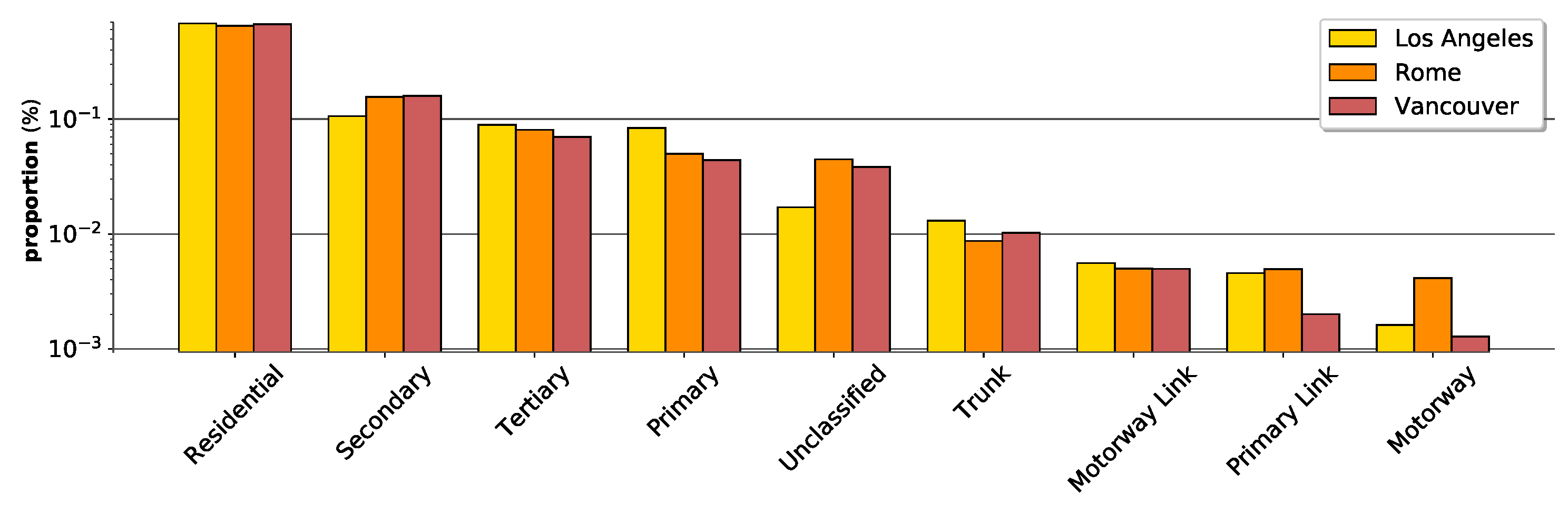
In this article, we consider street networks as spatial networks. Generally, graphs are deemed unstructured in the sense that topological features such as node degree are unbounded. However, this is not necessarily the case for street networks as there can only be a certain number of streets adjacent to one street. In addition, street networks are less dense than traditional networks. For example, the average degree of street networks in Los Angeles, Rome, and Vancouver are 4.47, 4.13, and 4.98 respectively. In comparison, a citation network, a social network and protein-protein interaction (PPI) graphs have an average degree of 9.15, 492, and 28.8 respectively [13]. Furthermore, street networks exhibit volatile homophily [14]. This phenomenon can be better understood through the concept of spatial polycentricity [15,16]. Using the distribution of street types across a city as an example, spatial polycentricity suggests that the street network of a city would not necessarily have the street classes clustered in sub-structures, hereby contradicting the general definition of homophily. In the same vein, street networks exhibit high class imbalance, with differences between two classes being as high as three orders of magnitude [7]

GNNs can be susceptible to overfitting and tend to be unpredictable when applied to real-world graphs [17,18]. This limitation is amplified when we consider the already discussed conflict between implementational assumptions of GNNs and the characteristics of street networks, especially in light of the extremely high variance between class distributions that exist in many spatial networks [7]. Thus, in this article, we study GNNs for node classification on street networks. Specifically, we seek to investigate the relationship between two pertinent characteristics of spatial networks to GNNs. These characteristics are a global graph structure and biased class distributions. Consequently, we formulate the following questions:

• How well do vanilla GNNs generalise on imbalanced spatial graphs?
• Can the performance of GNNs be improved by encoding knowledge about the global structure of the spatial networks?
• Can the generalisation capacity of GNNs be improved for imbalanced spatial graphs when global structure is accounted for?

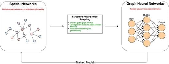
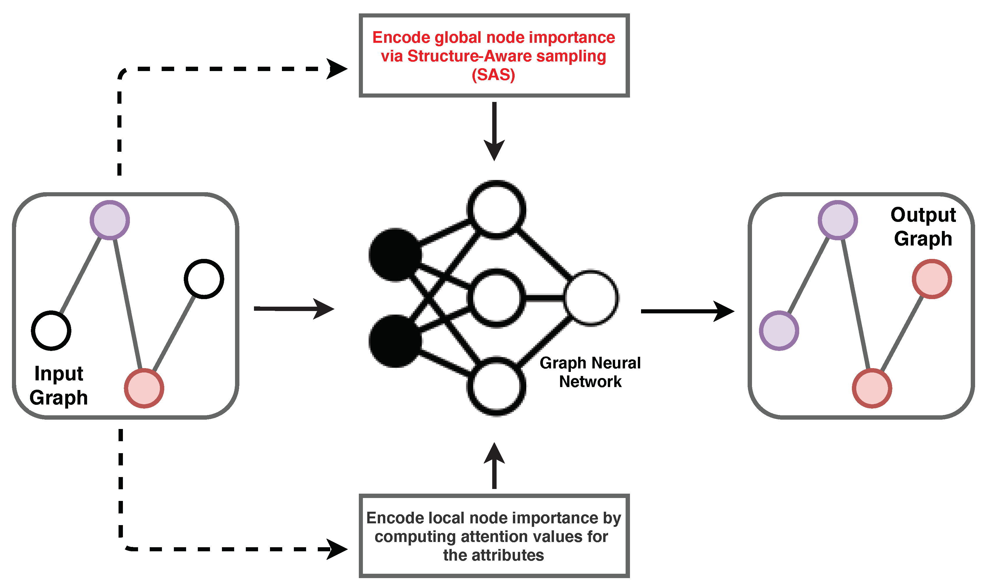
These questions are addressed in Section 7. We design our problem as a multi-class node classification one for graphs that are highly imbalanced. Specifically, we focus on the open research problem of enriching the semantics of spatial networks [7,8]. In this regard, we propose a new sampling approach: Structure-Aware Sampling (SAS), which encodes the global graph structure in the model by leveraging the intra-class and global-geodesic distances between nodes. We develop a neural framework using this sampling technique to train a model for spatial graphs. We evaluate our proposal against state-of-the-art methods on large real-world spatial graphs. Our results show a clear improvement in the majority of cases, with as much as a 20% F1-score improvement on average over traditional methods. Our approach is summarised in Figure 1.

We summarise our contributions succinctly:

• We show that vanilla GNNs fail to generalise sufficiently for imbalanced spatial graphs;
• We propose a new sampling technique (SAS) for training GNNs for spatial networks, which significantly improves model capacity;
• We demonstrate that encoding graph structure (via our sampling technique) to train GNNs improves the generalisability of models by an average F1-score of 20%, even with class imbalance.

The remainder of this article is organised as follows: In Section 2, we describe related themes and approaches. Preliminaries are defined and the problem formulated in Section 3. We describe our approach in Section 4 and experimental methodology in Section 5. We present and discuss our results in Section 6. We summarise our conclusions in Section 7.

2. Related Work

Our work in this article spans two broad research areas: Graph Neural Networks (GNNs) and semantic enrichment of spatial networks. GNN approaches can be described by the nature of the problems they solve, such as node classification, link prediction, or graph classification. Our scope in this article is limited to node classification and we review relevant works.

2.1. Graph Learning Approaches

Neural approaches for graphs aim to learn a representation for a node using a defined locality. This premise is inspired both by the success of traditional neural approaches and a need for their extension to unstructured domains such as graphs [1]. Broadly, GNNs can be grouped into: Spectral and spatial approaches. Spectral GNNs utilise the idea of convolutions [9] in the fourier domain through operations on the graph laplacian matrix [11,19,20,21]. These operations are computationally expensive and raise practical issues with scalability [11]. On the other hand, spatial approaches compute representations using an aggregation of neighbourhood features [12,13]. Attention-based methods are a variant of GNNs that rank the importance of information collected from neighbours of a node through the computation of an attentional value [12]. They have out-performed state-of-the-art methods and shown robustness on noisy real-world graphs [12,22]. We use an attention-based, spatial GNN approach in this article which is described in Section 4.

The literature of GNNs for spatial networks is still developing and there are currently very few relevant works. In [14], the authors propose a network that learns by embedding the between-edge and edge attributes of spatial networks. They apply this to tasks such as driving speed prediction and speed limit classification. However, they regard the spatial network as directed while we embed the directedness of the network in its attributes. Furthermore, we use a richer set of attributes for each node. The work done in [23] proposes a spectral-based GNN for traffic forecasting. Their network leverages the spatial-temporal dependency between entities during training. Their implementation focuses on the temporal aspects of these networks and is not directly comparable to our scope in this article. To the best of our knowledge, our article is the first that attempts to improve the robustness of GNNs on attributed spatial networks for node classification, specifically with consideration for their biased, multi-class nature.

2.2. Semantic Enrichment of Spatial Networks

The use of machine learning to enrich the semantics of spatial graphs is not new. A noteworthy focus of this research endeavour has been in the inference of map data. We adapt the definition of semantics from [6] as the descriptive details about spatial objects, e.g., the class of streets (motorway and secondary streets) and the use of buildings (residential and commercial buildings). In [5], they attempt to predict the semantics of streets on OpenStreetMap using their geometry. In [24], they propose weakly- and semi-supervised segmentation models for building maps. In [6], they propose transferable models for enriching map semantics while [7] exploits the use of contextual information to predict the semantics of streets on OpenStreetMap. However, a unifying characteristic of these approaches is their disregard for the relational dependence between entities [1,5,6,25,26,27,28]. GNNs present an opportunity to bridge this gap. We recognise the recent work done in [8] where the authors demonstrate a hybrid method consisting of a CNN and GNN for predicting the semantics of map data. Nonetheless, their scope is limited to only two street classes. This disregards the problem of biased classes in multi-class spatial graphs, which is more representative of real-world scenarios. Our work addresses this by considering nine street classes and proposes a solution for training GNNs to enrich the semantics of spatial networks when the class sizes are highly biased.

3. Preliminaries

3.1. Notations

We summarise the notations used in this article in

Table 1. Table of notations used and their definitions.

Notation	Definition
$\mathcal{G}=(\mathcal{V},\mathcal{E})$	An undirected spatial graph
$\mathcal{V}$	set of nodes in graph
$\mathcal{E}$	set of edges in graph
N	$\left|\mathcal{V}\right|$ number of nodes in $\mathcal{G}$
$\mathbf{H}$	set of attributes for nodes of $\mathcal{G}$
$\mathcal{Y}$	set of class labels for nodes in $\mathcal{G}$
$\mathbf{I}\left(\upsilon \right)$	importance of a node
LeakyReLU	The Leaky ReLU activation function
$\mathcal{F}\left(·\right)$	Learnt function
${\mathcal{N}}_i$	Neighbourhood of a node ${\upsilon }_i$

with their definitions.

3.2. Problem Formulation

Let $\mathcal{G}=(\mathcal{V},\mathcal{E})$ represent a homogeneous, unweighted, undirected, connected, multi-class, attributed spatial graph of size $N=\left|\mathcal{V}\right|$ with nodes ${\upsilon }_i\in \mathcal{V}$ and edges $({\upsilon }_i,{\upsilon }_j)\in \mathcal{E}$. The attributes of the nodes in $\mathcal{G}$ is denoted by $\mathbf{H}=\{{\overrightarrow{h}}_1,\cdots ,{\overrightarrow{h}}_N\}\in {\mathbb{R}}^{N\times r}$, which holds an $r$-dimensional real vector representation of the attributes $\forall \upsilon \in \mathcal{V}$. The class labels of $\mathcal{V}$ is given by $\mathcal{Y}=\{y_1,\cdots ,y_c\}\in {\mathbb{R}}^c$, where c is the number of class labels that exist in $\mathcal{G}$. We consider nine classes in this article. Our goal is to build a function $\mathcal{F}\left(·\right)$ that is given a graph $\mathcal{G}$ and a subset of $\mathcal{V}$ with its mapped attributes from $\mathbf{H}$, transductively learning the mapping between $\mathcal{V}$ and $\mathcal{Y}$.

3.3. Graph Neural Networks

A Graph Neural Network (GNN) is a neural network that learns directly on the graph structure. This paradigm achieves this by leveraging local information within the neighbourhood of a node [9]. This local information is represented either using message passing or neighbourhood aggregation [11,12,29]. The general form of a GNN is a neural network that takes a graph $\mathcal{G}=(\mathcal{V},\mathcal{E})$ as input and a real-valued set of attributes $\mathbf{H}=\{{\overrightarrow{h}}_1,\cdots ,{\overrightarrow{h}}_N\}\in {\mathbb{R}}^{N\times r}$. In this instance, we assume $\mathbf{H}$ is mapped to the nodes of $\mathcal{G}$ but could also be mapped to edges, depending on the case. The attributes are used by the neural network to create a representation for the nodes that leverages information in the local neighbourhood of a node ${\mathcal{N}}_i$. Our implementation performs neighbourhood aggregation of features for node ${\upsilon }_i$. Then, the GNN computes attention values for the aggregated information from the neighbours. This way, it is able to quantify which neighbour-features to emphasise or not. An activation function is applied to the combination of these values and their features and is passed to the next layer in the network. Hence, the representation of every node is a function of its neighbourhood. The final layer of GNNs will consist of an activation function that acts on the representations passed from the previous layer to compute the class probabilities. In this article, we use the softmax activation function [30], which is suitable for our multi-class classification problem.

4. The Proposed Model

In this article, we propose a method called SAS-GAT: Structure-Aware Sampling-Graph Attention Networks. We use this network to train a model for node classification on street networks, where the nodes denotes the street segments and the model learns a function to predict their class. We describe the components of the proposed architecture.

4.1. Structure-Aware Sampling (SAS)

The first component of our architecture is a sampling process that is designed to improve the generalisation power of the network. We propose to encode knowledge about the graph structure in our neural network by sampling the most important nodes for training. Given the multi-class nature of the graphs in our scope, we address this by leveraging the intra-class and global-geodesic distances of nodes in the graph. We refer to class here as the attribute label possessed by a node in a graph. In this article, the labels are the street types. It has been established that the influence or importance of a node can be deduced from its position in the graphs [31]. Similarly, different network measures can be used to quantify either the local or global importance of a node. Thus, we express the importance of a node in a multi-class spatial graph as follows:

$$\mathbf{I}\left(\upsilon \right)=\frac{1}{2}\sum (\mathcal{C},\mathcal{B}).$$

(1)

Here, $\mathbf{I}\left(\upsilon \right)$ denotes the importance of node $\upsilon$, $\mathcal{C}$ represents the intra-class distances, and $\mathcal{B}$ represents the global-geodesic distances. The key idea behind Equation (1) is to sample nodes that are not only influential within their class but are also important in the global structure of the graphs. It follows then that we adapt the closeness and betweenness centrality measures to model $\mathcal{C}$ and $\mathcal{B}$ respectively [32]. We extend the general form of the closeness centrality as defined in Equation (2) to consider class distributions. Hence, the closeness centrality of a node ${\upsilon }_i^{\ast }$, where ∗ denotes the class given by:

$$\mathcal{C}\left({\upsilon }_i^{\ast }\right)=\frac{N^{\ast }}{{\sum }_{{\upsilon }_j^{\ast }\in {\mathcal{V}}^{\ast }}d({\upsilon }_i^{\ast },{\upsilon }_j^{\ast })}$$

(2)

where $d\left(·\right)$ is the distance between two nodes, N, $\mathcal{V}$ as defined in Section 3.1. In this article, we consider the ${\mathcal{V}}^{\ast }$ of any class to be the largest set of connected nodes of that class. The betweenness centrality is defined thus:

$$\mathcal{B}\left({\upsilon }_i\right)=\sum _{m,n\in \mathcal{V}}\frac{\gamma (m,n|{\upsilon }_i)}{\gamma (m,n)}$$

(3)

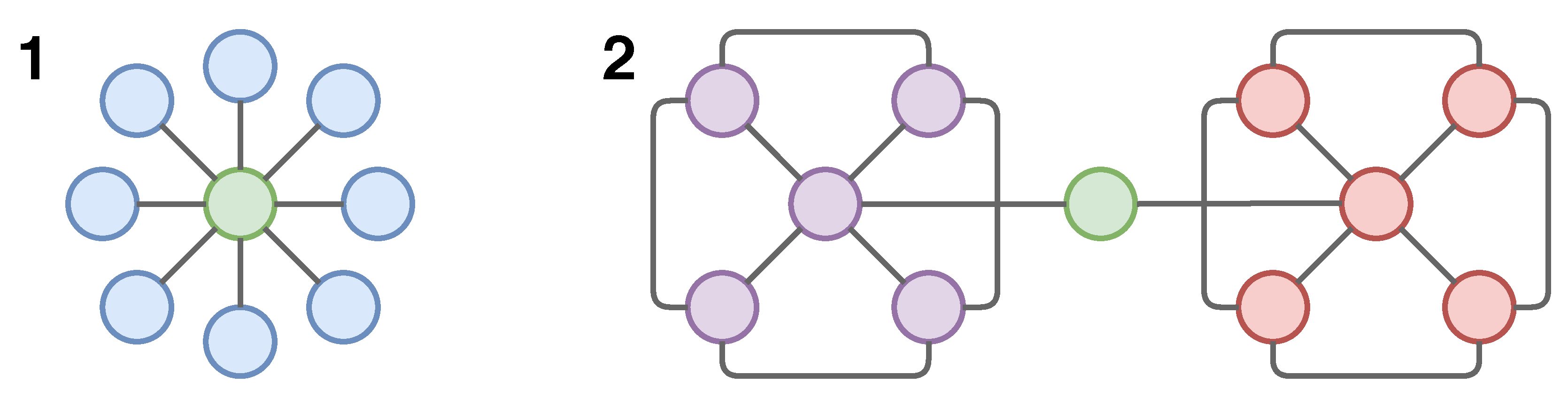
$\gamma (m,n)$ is the number of $m,n$-shortest paths in $\mathcal{V}$, and $\gamma (m,n|{\upsilon }_i)$ is the proportion of such shortest paths that go through ${\upsilon }_i$. Given the complexity of this measure, especially for large graphs, we adapt the approximation technique described in [33]. In this article, we implement this by using only 25% of the graph nodes. We present an intuitive visual description of both measures as it relates to multi-class graph structures in Figure 2. Finally, we normalise the values from Equations (2) and (3) before computing Equation (1).

We describe the computational implementation of Equation (1) in Algorithm 1. This algorithm takes as input the graph structure $\mathcal{G}$, the set of training nodes ${\mathbf{V}}_T$, the class labels for nodes $\mathcal{Y}$, and the set of per-class threshold values $\mathcal{K}$, $\mathcal{C}\left(·\right)$ and $\mathcal{B}\left(·\right)$ are as defined in Equations (2) and (3). B and C are normalised by setting their values in the range (0, 1). This algorithm returns a set of top-k nodes based on the preset thresholds ($\mathcal{K}$) for each class.

Algorithm 1: Sample Nodes using SAS

4.2. Aggregating Node-Level Neighbourhood Information with Attention

Having sampled the most important nodes via SAS, we proceed to exploit local node information. In this regard, we build upon the node attentional approach for graphs (GAT: Graph Attention Networks) described in [12] to develop our network. This approach allows for the computation of similarities between nodes using their attributes. However, this approach is naive about global graph structure which could be detrimental to model capacity. Therefore, in our neural architecture, we extend it by encoding global graph information as described in Section 4.1. Now, we describe the use of node level attributes to implement an attention mechanism.

Given a set of node features $\mathbf{H}=\{{\overrightarrow{h}}_1,\cdots ,{\overrightarrow{h}}_N\}$ from a graph network $\mathcal{G}$, where ${\overrightarrow{h}}_i\in {\mathbb{R}}^r$ and r is the number of features in the nodes $\upsilon \in \mathcal{V}$, we set $\mathbf{H}$ to the attributes that correspond to the nodes returned by Algorithm 1. This can be thought of as a subset of all node features. We implement an attention mechanism a by firstly performing a linear transformation $\mathbf{W}{\overrightarrow{h}}_i$ on the features of a node ${\overrightarrow{h}}_i$. If $y_i=\mathbf{W}{\overrightarrow{h}}_i$, then we can compute the attention value for any two pairs of nodes ${\upsilon }_i,{\upsilon }_j$ that share an edge as:

$$e_{ij}=a(y_i,y_j).$$

(4)

The attention values between any pair of nodes is normalised using the softmax function, thus:

$${\alpha }_{ij}={\mathrm{softmax}}_j\left(e_{ij}\right)=\frac{\exp \left(\mathrm{LeakyReLU}\left({\overrightarrow{\mathbf{a}}}^T\left(y_i\Vert y_j\right)\right)\right)}{{\sum }_{k\in {\mathcal{N}}_i}\exp \left(\mathrm{LeakyReLU}\left({\overrightarrow{\mathbf{a}}}^T\left(y_i\Vert y_k\right)\right)\right)}.$$

(5)

Here, $\overrightarrow{\mathbf{a}}$ is a weight vector, $·{}^T$ is the transpose, ‖ is the concatenation operator, and ${\mathcal{N}}_i$ is the neighbourhood of a node ${\upsilon }_i$. For the purpose of this article, we only consider direct neighbours of a node i.e one-hop. Next, the normalised attention values are fed to the next layer as a linear combination of the node features they represent, through a non-linear function $\sigma$ (we use the softmax in this article) expressed thus:

$${\overrightarrow{h}}_i^{\prime }=\sigma \left(\sum _{j\in {\mathcal{N}}_{\mathcal{i}}}{\alpha }_{ij}·y_j\right).$$

(6)

Furthermore, Equation (6) can be extended using multiple independent attention mechanisms as follows:

$${\overrightarrow{h}}_i^{\prime }={\Vert }_{k=1}^K\sigma \left(\sum _{j\in {\mathcal{N}}_{\mathcal{i}}}{\alpha }_{ij}^k·y_j^k\right).$$

(7)

Here, K denotes the number of independent attention mechanisms, ‖ represents the concatenation operation, ${\alpha }_{ij}^k$ denote the normalised attention values returned by the $k$-th attention mechanism, and $y_j^k$ is the corresponding weight matrix. We set K to eight attention mechanisms in our network. This value of K produced the most stable results in our preliminary investigations. Nonetheless, we show results for other number of attention mechanisms in Section 6. Using the multiple attention mechanism, we do not concatenate the transformations of each mechanism at the final layer. Rather, we compute their average before applying the non-linear softmax function ($\sigma$) as in [12]. See Figure 3 for a description of our neural framework.

5. Experiments

We carry out experiments, evaluating the proposed model against state-of-the-art methods. This section is a description of the experimental design employed in this article.

5.1. Data Description

The data used in our experiments were collected from OpenStreetMap (OSM). We use the street networks of three cities—Los Angeles, Rome, and Vancouver collected via the OSMNx API [34]. These cities span three countries and two continents, representing a diverse array of street patterns which formed the basis for their selection [6,7,35,36]. The original networks encoded the streets using an edge−edge representation, with each edge denoting a street. We transform this representation to its node−node equivalent using the line graph algorithm [37]. Essentially, this means that $N=\left|\mathcal{V}\right|=\left|\mathcal{E}\right|$. Where, N and $\left|\mathcal{V}\right|$ is the number of nodes in the transformed node−node representation and $\left|\mathcal{E}\right|$ is the number of edges in the original network. Each street network is a topological graph where the nodes represent street entities and the edges between nodes represent an intersection between streets. Note that the graph representation of each network is an undirected multigraph. Information about the directedness of each street, i.e., whether it is one-way or not is encoded into the graph using the node attributes. We attribute the nodes with a rich array of contextual information using the fixed multiple buffer approach described in [7]. We describe this approach below in Section 5.2. We consider nine road labels: Residential, secondary, primary, trunk, primary link, tertiary, unclassified, motorway link, and motorway. It is important to mention that all the graphs were connected.

We show the class distributions of the graphs in Figure 4. Here, we can see the high variability between classes in each graph. Recall that this is a key motivation of our proposal. In

Table 2. Summary of datasets.

	Los Angeles	Rome	Vancouver
No. of nodes	73,899	59,106	12,474
No. of edges	165,194	122,220	31,119
Average degree	4.47	4.13	4.98
Density	6.049 × 10${}^{-5}$	6.997 × 10${}^{-5}$	0.0004
No. of attributes per node	278	358	358
No. of class labels	9	9	9

, we present summary statistics of the datasets. As mentioned in Section 1, we see that the average degree is ≤ 5. In addition, it is worthy to mention that the density of these graphs are very low. The density values range between 1—High (very connected, clustered) and 0—Low (very spread out).

5.2. Attributing Graph Nodes

We attribute the graph nodes using descriptive information about the street by employing the fixed multiple buffer approach described in [7]. We collect the count of pre-determined objects within multiple buffers laid over each street. The buffers are polygons with rounded corners which take the shape of the streets. The buffers are polygons with holes, with the exception of the first polygon. For our experiments, we set the radii of the polygons to range from 10 m to 1000 m. The set of objects considered within the buffers is outlined in

Table 3. OpenStreetMap (OSM) descriptive tags used to attribute the graph nodes.

Tag Type	Tag Values
Amenity	parking, bench, school, restaurant, fuel, cafe, bank, bicycle parking, bar, pub, parking entrance, library, community centre, marketplace
Building	house, apartments, residential, garage, detached, industrial, commercial, terrace
Land Use	residential, farmland, industrial, commercial, retail, recreation ground, railway
Shop	department store, convenience, supermarket, mall
Service	driveway

. In OSM, descriptive information about objects is grouped using tag types. Each tag type can hold multiple tag values. We consider five tag types and 34 tag values. Additionally, we include descriptive information about the streets collected from OSM such as the length of the streets and a boolean value which denotes if the node is a one-way street or not. The total number of attributes for each graph is given in Table 2. The disparity recorded for Los Angeles is due to the unavailability of some tag values collected for other cities.

5.3. Model Training Strategy

We train our neural network described in Section 4 using Algorithm 2 for 100 epochs. Our architecture is a 2-layer feed-forward network with one hidden layer adapted from the attentional layer described in [12]. The output of the hidden layer is activated using the Exponential Linear Unit (ELU), the softmax activation is applied to the final layer to produce class probabilities [30]. We set the learning rate, $\lambda =1\times {10}^{-3}$, it is worthy to mention that this value produced the best results in our initial experiments. Our loss function is the cross-entropy loss and is minimised using the Adam optimisation rule [38] in PyTorch [39]. For experimental purposes, we trained the network using the following number of attention heads $\{2,3,4,6,8,10\}$.

The nodes used for training are selected using Algorithm 1. The validation and test nodes are set before train time. In our experiments, we set the number of validation and test nodes for each city to be equal for all the models. Thus, despite the variance in the number of class sizes, this uniformity will allow for an objective insight into the performance of each model. We preset the size of the validation and test nodes as a function of the least occurring class in each dataset. We impose early-stopping during model training by saving the best model, which are used for evaluations later. Note that the best model is evaluated using the validation nodes. The model is validated at each epoch using the set of validation nodes defined by the mask ${\mathcal{V}}_v=\rho \left(\mathcal{G}\right)$. The mask is a set of boolean values that describes the nodes to select. The model evaluation is presented using the test nodes in Section 6.

Algorithm 2: Model Training.

Furthermore, we train the models in two ways: Balanced and proportional. For the former, we ensure that the train nodes are balanced, down-sampled to the least occurring class. For the latter, we select a sample of the train nodes for each class as a proportion of its size in the graph. This 2-way training approach is designed to represent both an ideal (balanced) case and the biased class case (proportional). From Algorithm 2, $\tau$ is defined separately for both training approaches based on class size or the balanced case, while $\rho$ remains the same for all experiments. We present the results for these experiments in Section 6. The neural networks are implemented using PyTorch [39].

5.4. Baseline Methods

In addition to evaluating our proposal against GAT [12], we compare our proposal two state-of-the-art methods: GCN [11] and GraphSAGE [13]. Both methods are implemented in this article by training for 100 epochs. We evaluate trained models on the validation set and save the best performing one. The hyper-parameters outlined here were selected after an initial performance evaluation. The cross-entropy loss is minimised using the Adam optimisation rule.

5.4.1. Graph Convolutional Network (GCN)

We implement the Graph Convolutional Network proposed in [11]. Our network is a 2-layer feed forward network with 16 hidden features. We use the $RELU$ activation function for the hidden layer. During training, we use the $L_2$ regularisation with $\lambda =0.0001$. The final layer is activated using the softmax function.

5.4.2. GraphSAGE

We set up the network proposed in [13] as a 3-layer feed forward network with 16 hidden features. The activation function for the hidden layers is the $RELU$ and softmax for the output layer. The neighbourhood aggregation scheme used is the mean. We set the learning rate $\lambda =0.001$.

5.5. Algorithmic Complexity

The computational cost of using multiple attention heads (K) in our neural framework increases the memory and time requirements by a factor of K. Furthermore, the computation of Equation (1) requires a traversal of the nodes in the graph at least once. Particularly, this could become really expensive when computing $\mathcal{B}$, requiring $\Theta \left({\mathcal{V}}^3\right)$ time using a naive approach. In our implementation, we approximate $\mathcal{B}$ using the approach described in [33] with a 25% sample of the graph nodes. This reduces the time requirement to $\mathcal{O}\left(\mathcal{V}·\mathcal{E}\right)$, where $\mathcal{V}$ and $\mathcal{E}$ denote the number of nodes and edges in the graph respectively. Nonetheless, this could still pose a challenge when computational resources are limited, and we recognise this as a possible limitation of our proposal.

6. Results

6.1. Evaluating the Trained Models

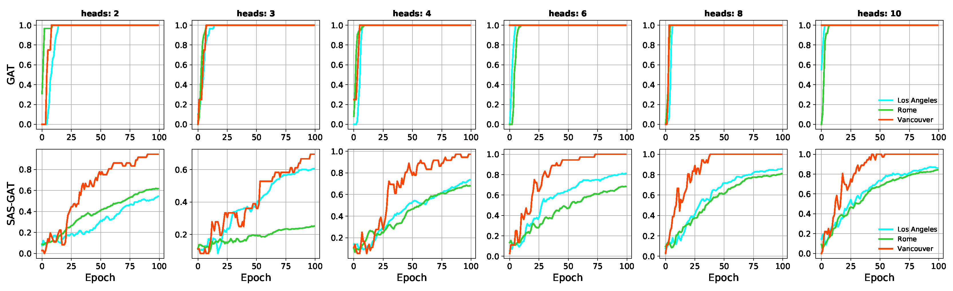
In Figure 5 and Figure 6, we present the model accuracies at train time. For brevity, we only show accuracies derived from models trained using a balanced set of train nodes. We compare models trained naively using the approach described in [12] against ours (SAS-GAT). In Figure 5, we can see the steady progression of the model as it converges. This is a clear contrast to the results of the performance of the GAT model which peaks rapidly. This observation is indicative of a model overfit, a recognised shortcoming of Graph Neural Networks [17].

We compare the trained models by evaluating them using the micro and macro-averaged F1-score. The general formula for the F1-score is given in Equation (8). Specifically, we compare the models trained with the balanced set of training nodes (see Section 5.3) using the micro F1-score. While, for the models built using the training nodes proportional to their class sizes, we use the macro F1-score as this measure penalises class sizes:

$$\mathbf{F}\mathbf{1}-\mathbf{score}=2\ast \frac{(precision\ast recall)}{(precision+recall)}.$$

(8)

We present the results in

Table 4. Summary of results for our method. We compare with GAT using the micro and macro F1-score (%). Results in sub-table (a) are achieved training using a balanced set of training nodes. Sub-table (b) denotes results achieved using a set of training nodes proportionate to the class size. Best results for each case are in bold.

Datasets	Los Angeles		Rome		Vancouver
Method	GAT	SAS-GAT	GAT	SAS-GAT	GAT	SAS-GAT
2H	15.2 ± 0.001	17.8 ± 0.001	9.3 ± 0.010	17.7 ± 0.003	8.3 ± 0.100	30.6 ± 0.012
3H	16.7 ± 0.110	13 ± 0.003	13.3 ± 0.013	18.4 ± 0.021	13.9 ± 0.111	25 ± 0.012
4H	11.9 ± 0.012	18.9 ± 0.010	10.9 ± 0.001	25 ± 0.025	13.9 ± 0.101	16.7 ± 0.101
6H	11.5 ± 0.190	17.8 ± 0.065	25 ± 0.192	31.3 ± 0.018	8.3 ± 0.010	19.4 ± 0.087
8H	7.8 ± 0.601	23 ± 0.013	9.3 ± 0.003	31.3 ± 0.006	11.1 ± 0.023	33.3 ± 0.021
10H	11.1 ± 0.011	21.9 ± 0.111	11.8 ± 0.901	30.2 ± 0.007	11.1 ± 0.072	30.6 ± 0.025
(a) micro F1-score
2H	3.7 ± 0.008	4.9 ± 0.072	8.6 ± 0.032	2.7 ± 0.012	4.4 ± 0.052	2.8 ± 0.094
3H	8.6 ± 0.002	10.3 ± 0.043	5.4 ± 0.021	5.7 ± 0.001	2.8 ± 0.012	19.7 ± 0.051
4H	3.5 ± 0.012	10.2 ± 0.001	9.1 ± 0.023	14.7 ± 0.022	3 ± 0.140	12.7 ± 0.011
6H	2.5 ± 0.020	11.5 ± 0.101	3.5 ± 0.005	8 ± 0.120	1.7 ± 0.059	20.3 ± 0.090
8H	3.5 ± 0.032	11.8 ± 0.020	6.8 ± 0.086	11.2 ± 0.049	4.5 ± 0.065	23.5 ± 0.094
10H	7.8 ± 0.011	13.2 ± 0.074	3.6 ± 0.091	11.8 ± 0.010	2.3 ± 0.005	19.6 ± 0.081
(b) macro F1-score

. In these Tables, we can see that the results are shown with respect to the number of heads used to train the model. The values in these tables are the averages taken after 10 iterations and their standard deviations are presented alongside. We see that in almost all cases, the standard deviation is negligible which shows that the results of our models are not random.

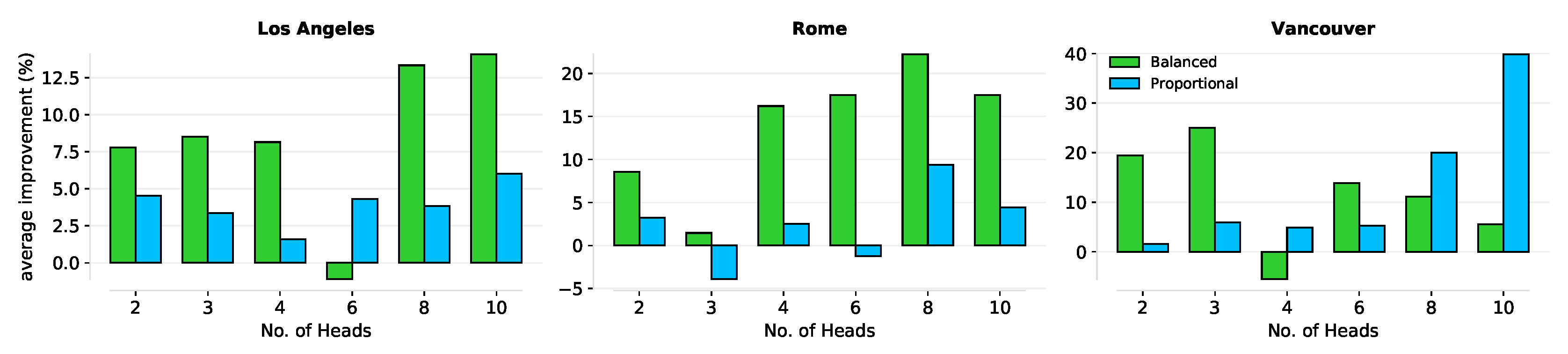
We highlight the performance of our neural framework using the proposed sampling technique in Figure 7. The values plotted in this figure are the average percentage improvement (F1-score) recorded from our neural framework. We show the cases for varying number of heads. It can be seen that the general improvement from using more attention heads is not affected by our approach. Overall, we can see that our proposal results in a more generalisable model compared to the traditional method.

6.2. Evaluating the Generalisability of GNNs

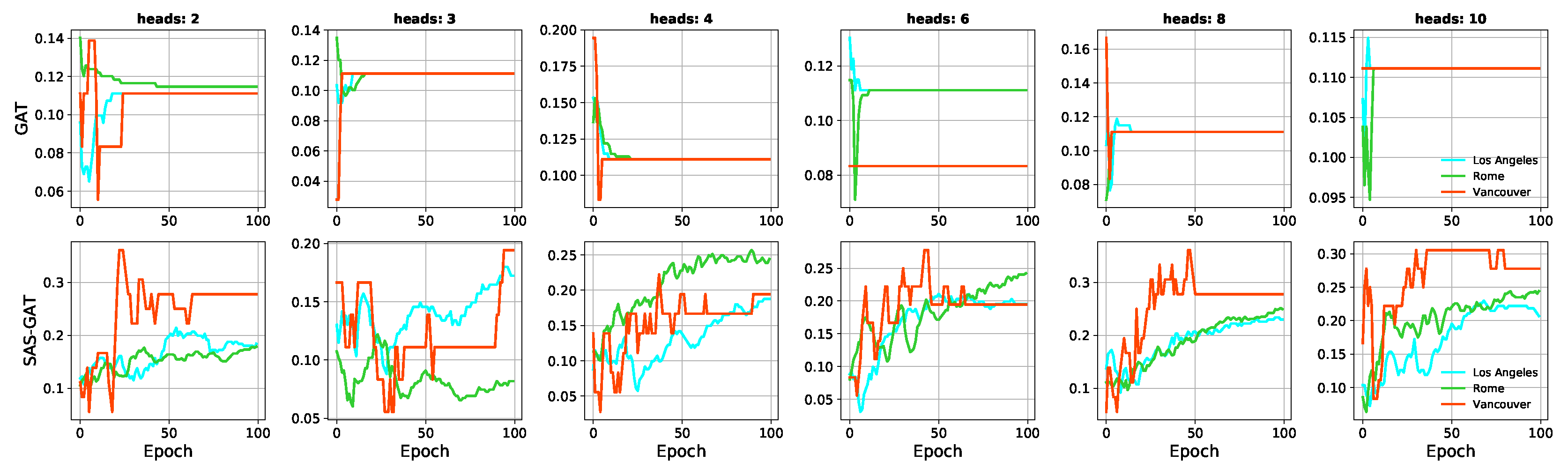
It can be seen from Figure 5 that the training accuracy of the vanilla GNN peaks rapidly within the first 20 epochs in all the cases. This behaviour is usually indicative that a model will overfit. Model over-fitting and over-smoothing have been identified as limitations of GNNs [17]. This is confirmed when we consider Figure 6 which holds the validation accuracy of the models. Here, we can see that our sampling enables the model to improve and generalise better with each epoch. It is worthy to reiterate that the same set of validation nodes are used for each dataset for all the models.

We evaluate the generalisation capacity in two dimensions: The balanced case and imbalanced case. We present the results in Table 4. In the former, the training nodes are balanced while in the latter, a proportion of the class sizes is used. We use two variants (micro and macro) of the F1-score to demonstrate these cases. Clearly and as expected, the balanced case produces better generalisations for all the datasets. However, we can see that in both cases, our neural framework generalises better. In the imbalanced case, where the variance between class sizes could lead the model to overfit on the majority class, we see that our sampling approach is able to mitigate this problem and produce superior results.

6.3. Comparing the Baselines

We evaluate our sampling technique on two other baselines: A Graph Convolutional Network as proposed in [11] and GraphSAGE [13]. For both methods, we incorporate our sampling technique. The model training is done on the same graph nodes used for other methods. We present a summary of results in

Table 5. Summary of results for the Graph Convolutional Networks (GCN) and GraphSAGE. We compare results with models trained using our sampling technique SAS-GCN and SAS-GraphSAGE. The metric used here is the micro and macro-averaged F1-score. Results presented are the averages.

Dataset	Los Angeles		Rome		Vancouver
Method	micro	macro	micro	macro	micro	macro
GCN	0.13	0.04	0.13	0.08	0.08	0.08
SAS-GCN	0.11	0.08	0.11	0.06	0.17	0.08
GraphSAGE	0.13	0.03	0.11	0.07	0.08	0.05
SAS-GraphSAGE	0.12	0.05	0.09	0.04	0.22	0.07

. Results presented are the micro and macro-averaged F1-scores. The micro F1-score metric is used for models trained using the balanced set of nodes, while the macro F1-score metric are used for the proportional case. We see that using our sampling technique (SAS) leads to better results in some cases. In addition, it is seen from the macro columns that our sampling technique generally improves performance when the class sizes are biased. Nonetheless, the performance of these models are not as impressive as the attention model (seen in Table 4). This observation suggests that attention models may be better suited for noisy real-world graphs [12,22].

7. Conclusions

In this article, we proposed a novel approach to sampling nodes when training Graph Neural Networks for spatial graphs. This work is motivated by a need to improve the generalisability of GNNs for noisy real-world graphs. Subsequently, the approach proposes to achieve this by encoding global graph structure into the model development process. It was implemented by leveraging the structure of the graph using intra-class and global-geodesic distances. The problem was formulated as a node classification with one for noisy, biased, and multi-class graphs. The approach was evaluated on three large real-world datasets that have a high variance between class sizes. Our evaluations showed that our sampling approach was able to mitigate the problem of over-fitting and over-smoothing observed in GNNs. In addition, we determined that our technique leads to a more generalisable model. Consequently, we addressed the questions posed in Section 1: (1) Vanilla GNNs do not generalise well on spatial graphs, at least not when compared to an approach using global structure. (2) The performance of GNN models could improve significantly when global structure is taken into consideration. (3) The generalisation capacity of GNN models can be improved when a global graph structure is considered.

The significance of our results is appreciated in light of the recent interest in graph neural methods among researchers. A limitation of traditional machine-learning methods is that they assume independence between entities. This makes them unsuitable in situations where entities share a relationship (i.e., exhibit dependence). Graph Neural Networks (GNNs) bridge this gap by preserving the relational dependence between entities during learning. However, the focus of GNNs on local neighbourhood with disregard for global structure could hamper model robustness for spatial graphs. We believe that our work in this article will inspire a broader investigation into improving GNNs for spatial tasks. In this article, we demonstrated the importance of global structure for learning on spatial graphs. For future work, we will investigate the transferability of our method across street networks.

References

- Battaglia, P.W.; Hamrick, J.B.; Bapst, V.; Sanchez-Gonzalez, A.; Zambaldi, V.; Malinowski, M.; Tacchetti, A.; Raposo, D.; Santoro, A.; Faulkner, R.; et al. Relational inductive biases, deep learning, and graph networks. arXiv 2018, arXiv:1806.01261. [Google Scholar]
- Li, J.; Cai, D.; He, X. Learning graph-level representation for drug discovery. arXiv 2017, arXiv:1709.03741. [Google Scholar]
- Tolstaya, E.; Gama, F.; Paulos, J.; Pappas, G.; Kumar, V.; Ribeiro, A. Learning decentralized controllers for robot swarms with graph neural networks. arXiv 2019, arXiv:1903.10527. [Google Scholar]
- Liu, Z.; Chen, C.; Yang, X.; Zhou, J.; Li, X.; Song, L. Heterogeneous graph neural networks for malicious account detection. In Proceedings of the 27th ACM International Conference on Information and Knowledge Management, Turin, Italy, 22–26 October 2018; pp. 2077–2085. [Google Scholar]
- Corcoran, P.; Jilani, M.; Mooney, P.; Bertolotto, M. Inferring semantics from geometry: The case of street networks. In Proceedings of the 23rd SIGSPATIAL International Conference on Advances in Geographic Information Systems, Bellevue, WA, USA, 3–6 November 2015; p. 42. [Google Scholar]
- Iddianozie, C.; McArdle, G. A transfer learning paradigm for spatial networks. In Proceedings of the 34th ACM/SIGAPP Symposium on Applied Computing, Limassol, Cyprus, 8–12 April 2019; pp. 659–666. [Google Scholar]
- Iddianozie, C.; Bertolotto, M.; Mcardle, G. Exploring Budgeted Learning for Data-Driven Semantic Inference via Urban Functions. IEEE Access 2020, 8, 32258–32269. [Google Scholar] [CrossRef]
- He, S.; Bastani, F.; Jagwani, S.; Park, E.; Abbar, S.; Alizadeh, M.; Balakrishnan, H.; Chawla, S.; Madden, S.; Sadeghi, M.A. RoadTagger: Robust Road Attribute Inference with Graph Neural Networks. In Proceedings of the Thirty-Fourth AAAI Conference on Artificial Intelligence, AAAI 2020, New York, NY, USA, 7–12 February 2020; pp. 10965–10972. [Google Scholar]
- LeCun, Y.; Bengio, Y. Convolutional networks for images, speech, and time series. Handb. Brain Theory Neural Netw. 1995, 3361, 1995. [Google Scholar]
- Karpathy, A.; Johnson, J.; Fei-Fei, L. Visualizing and understanding recurrent networks. arXiv 2015, arXiv:1506.02078. [Google Scholar]
- Kipf, T.N.; Welling, M. Semi-supervised classification with graph convolutional networks. arXiv 2016, arXiv:1609.02907. [Google Scholar]
- Veličković, P.; Cucurull, G.; Casanova, A.; Romero, A.; Lio, P.; Bengio, Y. Graph attention networks. arXiv 2017, arXiv:1710.10903. [Google Scholar]
- Hamilton, W.; Ying, Z.; Leskovec, J. Inductive representation learning on large graphs. In Proceedings of the Advances in Neural Information Processing Systems 30: Annual Conference on Neural Information Processing Systems 2017, Long Beach, CA, USA, 4–9 December 2017; pp. 1024–1034. [Google Scholar]
- Jepsen, T.S.; Jensen, C.S.; Nielsen, T.D. Graph convolutional networks for road networks. In Proceedings of the 27th ACM SIGSPATIAL International Conference on Advances in Geographic Information Systems, Chicago, IL, USA, 5–8 November 2019; pp. 460–463. [Google Scholar]
- Roth, C.; Kang, S.M.; Batty, M.; Barthélemy, M. Structure of urban movements: Polycentric activity and entangled hierarchical flows. PLoS ONE 2011, 6, e15923. [Google Scholar] [CrossRef] [Green Version]
- Barthélemy, M. Spatial networks. Phys. Rep. 2011, 499, 1–101. [Google Scholar] [CrossRef] [Green Version]
- Li, Q.; Han, Z.; Wu, X.M. Deeper insights into graph convolutional networks for semi-supervised learning. In Proceedings of the Thirty-Second AAAI Conference on Artificial Intelligence, Riverside, NO, USA, 2–7 February 2018. [Google Scholar]
- Rong, Y.; Huang, W.; Xu, T.; Huang, J. Dropedge: Towards deep graph convolutional networks on node classification. arXiv 2019, arXiv:1907.10903. [Google Scholar]
- Bruna, J.; Zaremba, W.; Szlam, A.; LeCun, Y. Spectral networks and locally connected networks on graphs. arXiv 2013, arXiv:1312.6203. [Google Scholar]
- Duvenaud, D.K.; Maclaurin, D.; Iparraguirre, J.; Bombarell, R.; Hirzel, T.; Aspuru-Guzik, A.; Adams, R.P. Convolutional networks on graphs for learning molecular fingerprints. In Proceedings of the Advances in Neural Information Processing Systems 28: Annual Conference on Neural Information Processing Systems 2015, Montreal, QC, Canada, 7–12 December 2015; pp. 2224–2232. [Google Scholar]
- Defferrard, M.; Bresson, X.; Vandergheynst, P. Convolutional neural networks on graphs with fast localized spectral filtering. In Proceedings of the Advances in Neural Information Processing Systems 29: Annual Conference on Neural Information Processing Systems 2016, Barcelona, Spain, 5–10 December 2016; pp. 3844–3852. [Google Scholar]
- Zhou, J.; Cui, G.; Zhang, Z.; Yang, C.; Liu, Z.; Wang, L.; Li, C.; Sun, M. Graph neural networks: A review of methods and applications. arXiv 2018, arXiv:1812.08434. [Google Scholar]
- Diao, Z.; Wang, X.; Zhang, D.; Liu, Y.; Xie, K.; He, S. Dynamic spatial-temporal graph convolutional neural networks for traffic forecasting. In Proceedings of the Thirty-Third AAAI Conference on Artificial Intelligence, Honolulu, HI, USA, 27 January–1 February 2019; Volume 33, pp. 890–897. [Google Scholar]
- Bonafilia, D.; Gill, J.; Basu, S.; Yang, D. Building High Resolution Maps for Humanitarian Aid and Development with Weakly-and Semi-Supervised Learning. In Proceedings of the IEEE Conference on Computer Vision and Pattern Recognition Workshops, Long Beach, CA, USA, 16–17 June 2019; pp. 1–9. [Google Scholar]
- Belgiu, M.; Tomljenovic, I.; Lampoltshammer, T.; Blaschke, T.; Höfle, B. Ontology-based classification of building types detected from airborne laser scanning data. Remote Sens. 2014, 6, 1347–1366. [Google Scholar] [CrossRef] [Green Version]
- Black, W.R. Network autocorrelation in transport network and flow systems. Geogr. Anal. 1992, 24, 207–222. [Google Scholar] [CrossRef]
- Chen, J.; Lai, C.; Meng, X.; Xu, J.; Hu, H. Clustering moving objects in spatial networks. In International Conference on Database Systems for Advanced Applications; Springer: Berlin/Heidelberg, Germany, 2007; pp. 611–623. [Google Scholar]
- Kaul, M.; Yang, B.; Jensen, C.S. Building accurate 3d spatial networks to enable next generation intelligent transportation systems. In Proceedings of the 2013 IEEE 14th International Conference on Mobile Data Management, Milan, Italy, 3–6 June 2013; Volume 1, pp. 137–146. [Google Scholar]
- Gilmer, J.; Schoenholz, S.S.; Riley, P.F.; Vinyals, O.; Dahl, G.E. Neural message passing for quantum chemistry. In Proceedings of the 34th International Conference on Machine Learning, ICML 2017, Sydney, NSW, Australia, 6–11 August 2017; pp. 1263–1272. [Google Scholar]
- Dunne, R.A.; Campbell, N.A. On the pairing of the softmax activation and cross-entropy penalty functions and the derivation of the softmax activation function. In Proceedings of the 8th Australia Conference on the Neural Networks 1997; Citeseer: Melbourne, Australia, 1997; Volume 181, p. 185. [Google Scholar]
- Oldham, S.; Fulcher, B.; Parkes, L.; Arnatkeviciute, A.; Suo, C.; Fornito, A. Consistency and differences between centrality measures across distinct classes of networks. PLoS ONE 2019, 14. [Google Scholar] [CrossRef] [Green Version]
- Freeman, L.C. Centrality in social networks conceptual clarification. Soc. Netw. 1978, 1, 215–239. [Google Scholar] [CrossRef] [Green Version]
- Brandes, U.; Pich, C. Centrality estimation in large networks. Int. J. Bifurc. Chaos 2007, 17, 2303–2318. [Google Scholar] [CrossRef]
- Boeing, G. OSMnx: New methods for acquiring, constructing, analyzing, and visualizing complex street networks. Comput. Environ. Urban Syst. 2017, 65, 126–139. [Google Scholar] [CrossRef] [Green Version]
- Shekhar, S.; Evans, M.R.; Kang, J.M.; Mohan, P. Identifying Patterns in Spatial Information: A Survey of Methods. Wiley Interdiscip. Rev. Data Min. Knowl. Discov. 2011, 1, 193–214. [Google Scholar] [CrossRef]
- Alexander, C. A City Is Not a Tree; Sustasis Press/Off The Common Books: White Salmon, WA, USA, 2017. [Google Scholar]
- Hemminger, R.; Beineke, L. Line Graphs and Line Digraphs, Selected Topics in Graph Theory; Lowell, W.B., Wilson, R.J., Eds.; The Academic Press: Cambridge, MA, USA, 1978. [Google Scholar]
- Kingma, D.P.; Ba, J. Adam: A method for stochastic optimization. arXiv 2014, arXiv:1412.6980. [Google Scholar]
- Paszke, A.; Gross, S.; Massa, F.; Lerer, A.; Bradbury, J.; Chanan, G.; Killeen, T.; Lin, Z.; Gimelshein, N.; Antiga, L.; et al. PyTorch: An Imperative Style, High-Performance Deep Learning Library. In Proceedings of the Advances in Neural Information Processing Systems 32: Annual Conference on Neural Information Processing Systems 2019, NeurIPS 2019, Vancouver, BC, Canada, 8–14 December 2019. [Google Scholar]
Figure 1.
A description of our proposed methodology for the transductive learning case. We perform node sampling using the global structure of the graph. The input to the Graph Neural Network (GNN) is a partially labelled input graph. The global graph structure and node attributes are used to train our network. The output graph is fully labelled, where the colours of the node denote class membership.
Figure 2.
A depiction of node influence in multi-class graphs. The colours denote membership of a node class. (1) The green node will have a high closeness centrality among the group of nodes. In this case, we assume they all belong to the same class. (2) The green node will possess a high betweenness centrality between the two class clusters. Here, the green node could belong to either node clusters.
Figure 3.
Description of our method. (A) The street network nodes are attributed using their contextual information. (B) The proposed sampling technique is used to select nodes based on their position in the graph. Nodes with bold lines are the sampled ones and nodes with dotted lines are their neighbours. The weight of the red lines indicates the strength of attention given to the information from a node.
Figure 4.
Distribution of street labels across the different cities. We see high variance between the different classes of streets. The y-axis is the proportion of each street class plotted on the scale.
Figure 5.
Plots showing the model training accuracy per epoch at train time. Each column represents the number of attention heads used to train the models. The rows hold the accuracies for GAT and our method.
Figure 6.
Plots showing the model validation accuracy per epoch for the validation set. Each column represents the number of attention heads used to train the models. The rows hold the accuracies for GAT and our method.
Figure 7.
Plots showing the average percentage improvement. Each plot represents the experimental results from each city and the lines denote whether the training nodes were balanced or a proportion of the original class size. We see an improvement of as much as 20% using our sampling approach.