Density-Based Spatial Clustering and Ordering Points Approach for Characterizations of Tourist Behaviour

Abstract

Knowledge about the spots where tourist activity is undertaken, including which segments from the tourist market visit them, is valuable information for tourist service managers. Nowadays, crowdsourced smartphones applications are used as part of tourist surveys looking for knowledge about the tourist in all phases of their journey. However, the representativeness of this type of source, or how to validate the outcomes, are part of the issues that still need to be solved. In this research, a method to discover hotspots using clustering techniques and give to these hotspots a data-driven interpretation is proposed. The representativeness of the dataset and the validation of the results against existing statistics is assessed. The method was evaluated using 124,725 trips, which have been gathered by 1505 devices. The results show that the proposed approach successfully detects hotspots related with the most common activities developed by overnight tourists and repeat visitors in the region under study.

1. Introduction

Destinations worldwide registered around 1.5 billion international tourist arrivals in 2019, an increase of 3.8% year-on-year [1]. Thus, tourist managers are interested in predicting future tourist movement behaviour of the different segments from the tourist market [2]. A tourist segment is a group that might require separate experiences or tourist marketing service mixes [3]. The use of crowdsourced GNSS (Global Navigation Satellite System) data has allowed for gaining insights from tourist behaviour in order to answer complex questions regardless of whether it is an urban or rural environment [4,5]. Some of these questions have direct economic implications for the tourist destination regions such as the search of hotspots where tourism activities are undertaken and their relation with the segments of the tourist market.

Tourism market analysis is a complex task due to the diverse group of active tourists involved. A management strategy used is the market segmentation, where tourist data are used by service managers to identify tourist segments looking for predicting future tourist behavior [2]. According to the literature, the segmentation of the tourist market has been done based on approaches, such as tourist benefits [6], craft selection criteria and shopping involvement [7], and seasonality [8]. In a previous work [9], the tourist market segmentation in the Province of Zeeland in The Netherlands was performed based on the staying time patterns identifying three tourist segments: External 24, tourists who spent less than 24 h in the Zeeland region in only one occasion; External long, those who spent longer than 24 h in the Zeeland region in only one occasion; and External recurring, those for whom multiple trips in and out of the Zeeland region were observed.

Traditionally, tourism statistics have been collected using paper-based surveys which are not able to capture longitudinal behaviour of a tourist. Nowadays, tourism campaigns collect tourist data using crowdsourced smartphones applications, such as Bucketfood [10] and the Zeeland App [11], which have advantages when knowledge about the tourist in all phases of the journey is essential. The use of smartphones as sensors allows us to collect data in large geographical (rural) areas, in (even) less visited areas, and continuously at any time of the day. Therefore, the spatial-temporal data preciseness is higher than for regular tourism statistics [12]. Crowdsourced tourism campaigns are setting up for gaining different insights such as tourist mobility flows, the use of different types of transport modes, number of visitors and their mobility patterns, understanding visitors mobility profiles, and potential incentives that might be used to influence users’ mobility behaviour. However, spatio-temporal big data analysis is required to convert the gathered data into valuable and meaningful insights.

In the literature, the spatio-temporal big data analysis has developed contributions such as new algorithms, methods, frameworks, approaches, and solutions to address specific domain challenges [13] to mine information in order to understand phenoms as human mobility from crowdsourced GNSS data [14,15,16]. In the tourist domain, the trajectory analysis [17] called the trajectory data mining has been used on specific fields such as tourism to discover for example urban or rural tourism movement patterns [4,5,8], being one of its goals to mine points of interest. To identify clusters (e.g., hotspots), spatio-temporal attributes have been used as part of the input data of processing chains that include data mining subprocesses to transform data into knowledge [18]. In [19], association rule learning is applied for pattern mining in tourist attraction visits to demonstrate the potential of ad-hoc sensing networks in the non-participatory measurement of small-scale movements. In [20], the authors consider different clustering approaches to detect individuals and collective hotspots. Their findings proved that OPTICS was the most robust algorithm against initial parameters, but parameter tuning and data representativeness were not evaluated. Nevertheless, these data-driven results need to be validated. In the literature, external datasources such as geo-semantic information [21], Google categories [22], and OpenStreetMaps [20], have been used to perform this task.

In this research, a method to detect hotspots from the crowdsourced data giving them a data-driven interpretation is proposed. A crowdsourced dataset which was collected from over 1500 participants, over a period of five months, in the touristic Province of Zeeland, The Netherlands, is used. Only trips performed by tourist that belong to the External long and External recurring tourist segments [9] are considered. The fundamental research contributions of this work are related to the following research question: (i) how can crowdsourced data and resulting clusters obtained using this type of data source be validated? (ii) what are the added insights that crowdsourced data can bring on top of the existing statistics? (iii) are there differences among the tourist segments in their activity patterns?

The remainder of this paper is organized as follows: Section 2 gives an overview of the geographic study area and the dataset description. The detailed methodology applied to discover clusters that represent hotspots is also included in this section. In Section 3, results are given, together with some insights about the tourist hotspot and tourism crowdsourced campaign. The discussion of the findings takes place in Section 4, and the conclusions of this research can be found in Section 5.

2. Materials and Methods

2.1. Geographical Study Area

In The Netherlands, the province of Zeeland (Figure 1) is one of the most visited provinces in terms of foreign tourists, but it is the least populous province of the country [23]. The tourists visit the province for the activities (Table 3) that can be developed. Geographically, Zeeland is situated in the southwest of The Netherlands and includes about 2930 square kilometers area composed of shores and islands. The province of Zeeland has 13 municipalities. According to the Statistics Netherlands, a Dutch governmental institution, known in Dutch as Centraal Bureau voor de Statistiek (CBS), the province registered more than 10 million overnight stays in 2017, and for the first time, the number of overnight stays by foreign tourist (non-Dutch) exceeded the number of overnight stays by Dutch people (non-residents) [24]. This research was carried out in this province which is number 6 in The Netherlands in terms of number of nights, and number 3 in terms of foreign tourists.

2.2. Dataset

In this research, the following datasets are used:

• Crowdsourced tourist dataset. The data were collected by the mobile crowdsourced application provided by the official regional tourist information agency VVV Zeeland (Province of Zeeland, The Netherlands). The target users were tourists visiting the province from May to September 2017. During this period, a total of 10,597 users downloaded the application, of which 1505 contributed their data. The active users contributed 124,725 trips (travelled path from the trip origin to the trip destination location), and 151,612 trip segments (parts of the trip made by single transport mode). In the dataset, each record represents a trip segment. A detailed description of attributes collected for each trip segment is given in

  Table 1. Description of the variables.

  Variable	Acronym	Description
  User’s ID	userid	Unique identifier assigned to the device during the installation of the Zeeland app. A user is linked with only one device.
  Start time	start	Timestamp when the trip segment started.
  End time	end	Timestamp when the trip segment ended.
  Mode of transportation	mode	Mode of transportation used in the trip segment.
  Distance	distance	Distance traveled between the trip segment’s starting and ending points measured in meters.
  Waypoints	waypoints	Trajectory of geographic locations (latitude, longitude) followed from the trip segment’s starting until ending point. Additionally, every geography location contains the timestamp when the measure was gathered.
  Duration	duration	Duration of the trip segment measured in seconds.

  .
• CBS dataset. This dataset consists of the statistics published by CBS about the tourists in accommodations of the Province of Zeeland [24]. The time period considered in the comparison is from July to September 2017. This external data source is used to measure the representativeness of the crowdsourced data.
• Land-use of The Netherlands. This dataset consists of the land-use file from The Netherlands published by CBS [25]. It contains digital geometry of land use such as traffic areas, buildings, and recreation areas. This external data source is used to complement the dataset to be able to to give a data-driven interpretation to the results.

  Table 2. Description of the land-use dataset fields.

  Field	Acronym	Description
  Property’s ID	BG2015	Unique identifier of a property.
  Land-use level 1	Hoofdgroep	Level-1 description of the land-use of a property. It represents the main land-use.
  Land-use level 2	Omschrijvi	Level-2 description of the land-use of a property.
  Length of the property	Shape_Leng	Representative of the length of the geometry’s property.
  Area of the property	Shape_Area	Representative of the length of the geometry’s property.

  shows the dataset fields.
• Validation dataset. NBTC-NIPO Research is a research company that specializes in vacation, leisure, and business travel research. One of their research projects is the Continuous Holiday Research, known in Dutch as ContinuVakantieOnderzoek (CVO). This project is a large-scale consumer survey into holiday behaviour in The Netherlands. In CVO 2015, which was carried out from 1 October 2014 to 30 September 2015, people who spent a tourist holiday in Zeeland were asked whether they undertook certain activities during their holiday. The top 10 of the activities of Dutch overnight tourists in Zeeland is shown in

  Table 3. Top 10 activities of Dutch overnight tourists in the Province of Zeeland [26].

  Rank	Purpose	Tourists
  1	Visit to the beach	82%
  2	Eating out	70%
  3	Take walks	66%
  4	Fun shopping	37%
  5	Swimming	35%
  6	Bike rides	35%
  7	Visit to nature reserve	29%
  8	Visits to interesting buildings	29%
  9	Sunbathing	15%
  10	Visit to the museum	9%

  . In this research, this external data source is used to validate the interpretation of the results.

2.3. Methodology

In this section, the proposed methodology is described. Figure 2 shows the processing chain since crowdsourced data are provided as input until meaningful hotpots are provided as an outcome. As follows, the different steps will be discussed in more detail.

2.3.1. Preprocessing Dataset

During the preprocessing stage, data cleaning is performed to exclude trip segments with missing data or empty fields. The trips are recreated using the valid trip segments in order to extract features such as the trip’s destination location. The trips where the destination location is out of the area under study are filtered out. Then, data transformation is performed to extract some features. First, reverse geocoding is applied to the origin and destination locations to obtain the name of the municipality origin and destination if the location points are inside the area under study, otherwise they will be empty. Second, for each trip, the staying time is computed as the time difference between the arrival destination time of the current trip and the departure time of the next trip. Finally, the destination location feature is converted from decimal degrees to the Universal Transverse Mercator (UTM) coordinate system to be able to use meters as a distance measuring unit during the following methodology stages. Additionally, using the tourist market segmentation performed in [9], the tourist segment which the user belongs to is added to each trip in order to filter out trips not performed by the External long and External recurring tourist segments. Figure 3 illustrates the trip destination geographic locations of the dataset with the indication of the study region.

In this dataset, there are 25,613 data points. Each one represents a trip’s destination location. A detailed description of attributes collected for each trip destination location is given in

Table 4. Description of the variables.

Variable	Acronym	Description
User’s ID	userid	Unique identifier of the user.
Destination location	destiny	Geographic location (latitude, longitude) of the trip’s destination.
Municipality origin	municipality_o	Municipality where the trip started. In case the trip started out from the area is set up as empty.
Municipality destination	municipality_d	Municipality where the trip destination is located.
Arrival time	end	Timestamp when the trip ended.
Weekend	weekend	Represents whether or not the trip occurred during a weekend.
Stay time	stay	Represents how long time (hours) exists between the arrival time and the starting time of the next registered trip.
Tourist segment	segment	Represents the user tourist profile: External long, External recurring.

.

2.3.2. Dataset Representativeness

This study focuses on hotspot detection to improve understanding of Zeeland visitors’ behavior. It aims to create a density-based clustering model. However, this kind of model is usually trained with historical data assuming that the variables used by the model will maintain the same behavior in the near future. Therefore, it is assessed whether the crowdsourced dataset is a representative dataset or not. Hence, a comparison of the data distributions between the number of tourists in tourist accommodations by each municipality of the Province of Zeeland registered in the Statistics Netherlands dataset, and the number of inbound trips by each municipality of the Province of Zeeland registered in the crowdsourced dataset was performed.

Before performing the comparison, both samples were standardized to bring them onto the same scale, centering the mean at 0 with standard deviation 1. The procedure for standardization can be expressed as follows:

$$x_{std}^{(i)}=\frac{x^{(i)}-{\mu }_x}{{\sigma }_x}$$

(1)

where ${\mu }_x$ and ${\sigma }_x$ represent the mean and the standard deviation of the attribute.

Then, the two-sample Kolmogorov–Smirnov test (K–S test) (Equation (2)), which is a non-parametric test of the equality of continuous or discontinuous, is used to assess whether or not both samples come from a population with the same distribution. This test quantifies the K-S distance that it is defined as the maximum vertical distance between the empirical distribution functions of two samples. This is defined as follows:

$$D_{n,m}=\underset{x}{max}|F(x)-G(x)|$$

(2)

where $F(x)$ is the observed cumulative distribution function of the first sample that has size n, and $G(x)$ is the observed cumulative distribution function of the second sample that has size m. If the K–S distance is small or the p-value is high, then both samples come from a population with the same distribution (null hypothesis).

2.3.3. Clustering Analysis

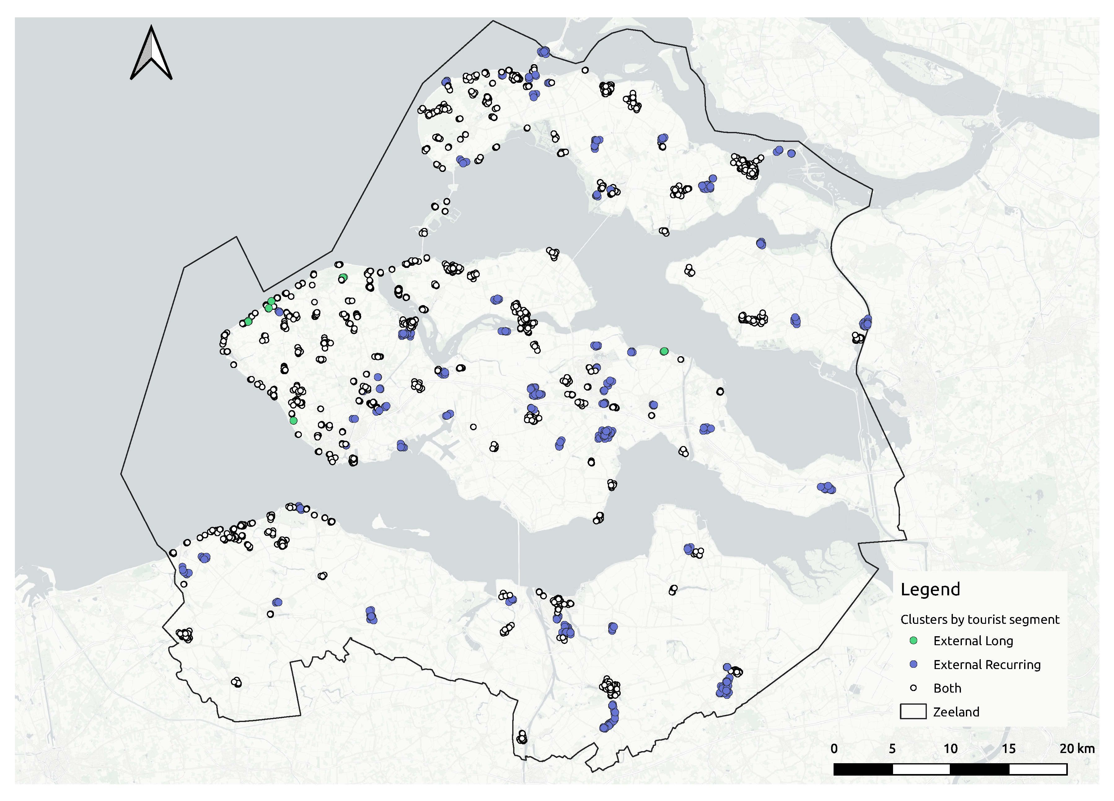
In this study, the aim is to identify hotspots visited by Zeeland tourists by using clustering, an unsupervised learning technique to explore data structures in order to extract meaningful information. A density-based clustering algorithm uses the concept of density which can be defined as the number of data points per unit volume of the feature space [27]. A data point is made from variables shown in

Table 5. Description of the variables for the clustering process.

Variable	Acronym	Description
Longitude	longitude	Represents the longitude component from the geographic location in UTM coordinate system.
Latitude	latitude	Represents the latitude component from the geographic location in UTM coordinate system.

. A region from the feature space is identified as a high-density or low-density area according to the occurrence of data points that are packed closely together. Then, clusters are identified by partitioning and learning patterns from high-density regions.

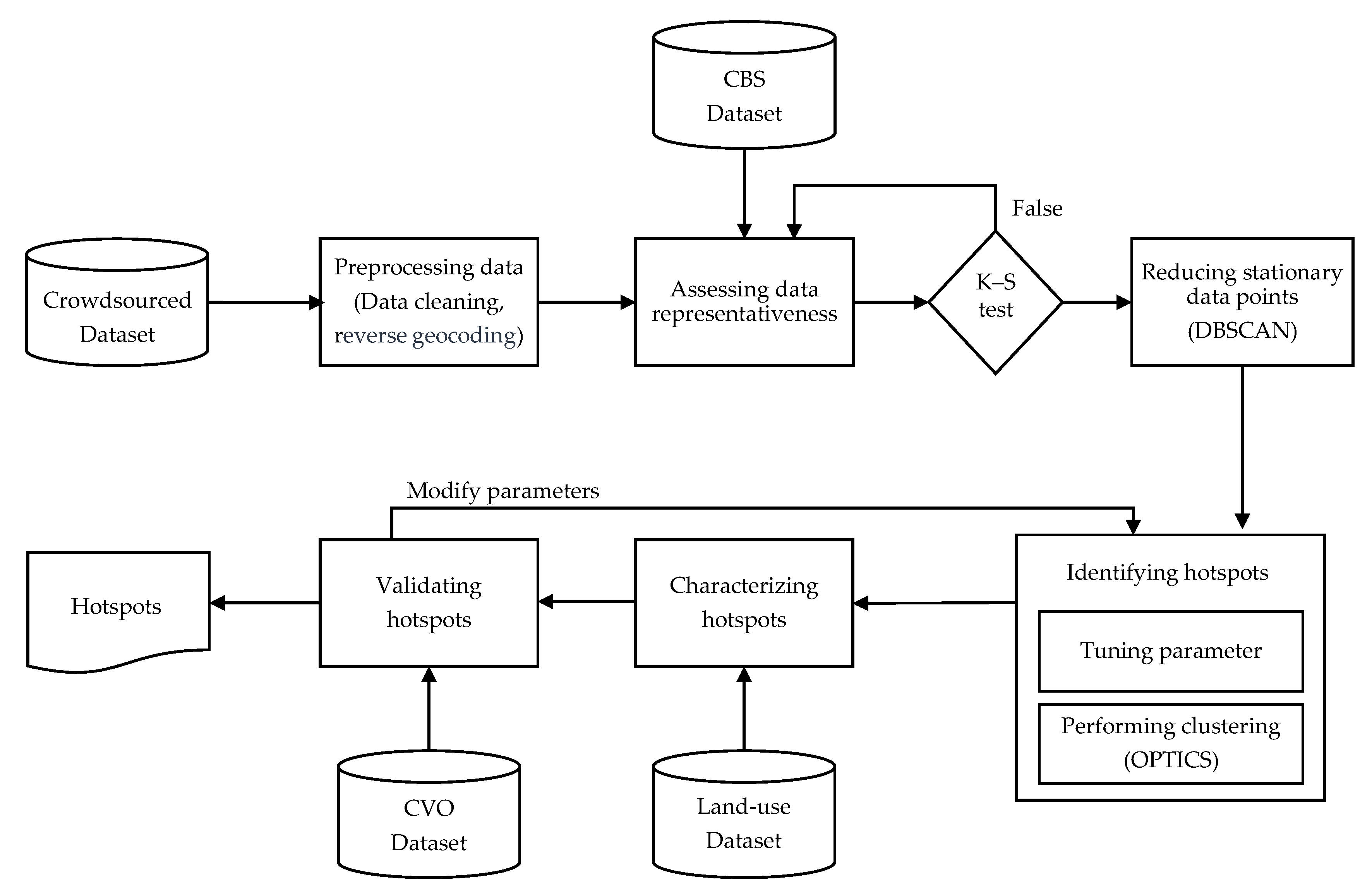
In this stage, the first aim is to reduce the number of data points generated by an individual tourist to then look for clusters with heterogeneous density. In general, the clustering algorithms do not consider the ownership of the data points, so a spot could be wrongly classified as a hotspot just because of the high number of visits registered by one single user. To handle this problem, the Density-Based Spatial Clustering of Applications with Noise (DBSCAN) algorithm [28] is selected as it finds places visited by a tourist regardless of how many times they were visited, i.e., clusters with any shape regardless their density, and because of DBSCAN’s ability to process very large datasets [29]. To handle the heterogeneous cluster density problem, the Ordering Points To Identify the Clustering Structure (OPTICS) algorithm [30] is used. The main advantage of OPTICS is that it can find clusters of varying density. To the best of our knowledge, density-based algorithms that handle both finding clusters with data points of different users and heterogeneous cluster density conditions do not exist. For example, the Reverse Nearest Neighbor-DBSCAN [31] that is an algorithm based on DBSCAN only handles the search for clusters with heterogeneous density. Photo-DBSCAN [32] finds clusters that contain data points of different users, but it does not guarantee that it can identify clusters with different densities.

DBSCAN has two parameters: the minimum number of data points to form a dense region (minPts) and ε (epsilon) that represents the maximum distance, expressed in units of the feature space, between two data points for one to be considered as in the neighborhood of the other. According to the literature, the number of dimensions (dim) of a dataset can be used to determine the hyperparameter minPts value. In many cases of a two-dimensional dataset, this can be kept at the default value of minPts = 4 [28], while in cases of large and high-dimensional datasets it can be set up minPts = 2*dim [33]. In some studies, a single absolute value is not suitable, so they have set it up based on a percentage of the data point ownership [34], using a heuristic approach based on the size of the dataset [35] or perform its value estimation using an objective function [36]. 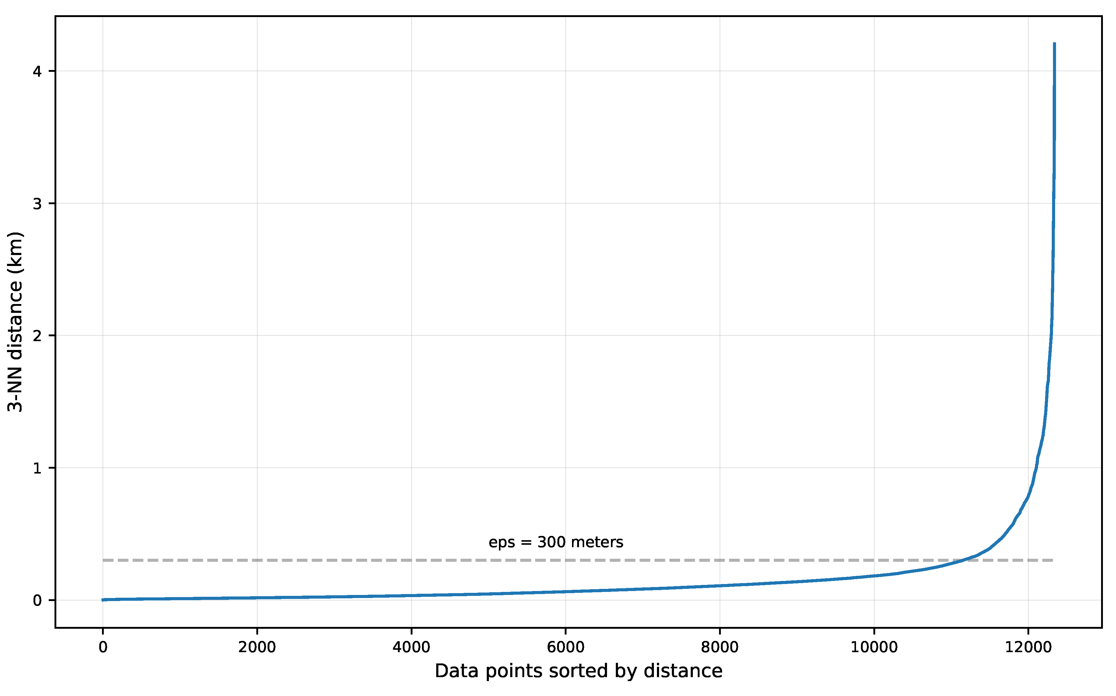In general, larger values of minPts are considered more robust to noise and produce more significant clusters. However, it is sought to represent the multiple visits made by a user to the same place with one single data point while places visited just once have to be kept, so non-data points should be classified as noise. The ε hyperparameter that represents the maximum distance of the search radius must be set up with the smallest possible value. This hyperparameter has also been tuned in many studies using the k-NN distance (i.e., 25 to 550 m) or considering the application domain and knowledge of the study area [33,36,37].

The algorithm starts by selecting a random data point p from the dataset D. Then, it looks for data points in the ε-neighborhood of p. If there are at least minPts data points (including it), p is marked as a core point representing the start of a cluster and all data points within its ε-neighborhood are added to its cluster. Otherwise, the data point p is labeled as noise; however, p might later be part of the ε-neighborhood of another core point and hence be made part of a cluster. The algorithm then visits each data point of the new cluster to perform the same task. If a point q from ε-neighborhood of p is a core point, these data points are said to be directly density connected and reachable from each other. The network made by these density-connected data points is considered a cluster. The algorithm searches recursively through the density connections from core points. It stops when a data point is reachable from a core point, but it is not a core point. This data point is considered a border point. Then, the algorithm continues by selecting an unvisited data point to repeat the process.

In DBSCAN, the default distance metric used for neighborhood computation is the Euclidean distance between two data points (Equation (3)). This is defined as follows:

$$dist(i,j)=\sqrt{{(x_{i1}-x_{j1})}^2+{(x_{i2}-x_{j2})}^2+\dots +{(x_{ip}-x_{jn})}^2},$$

(3)

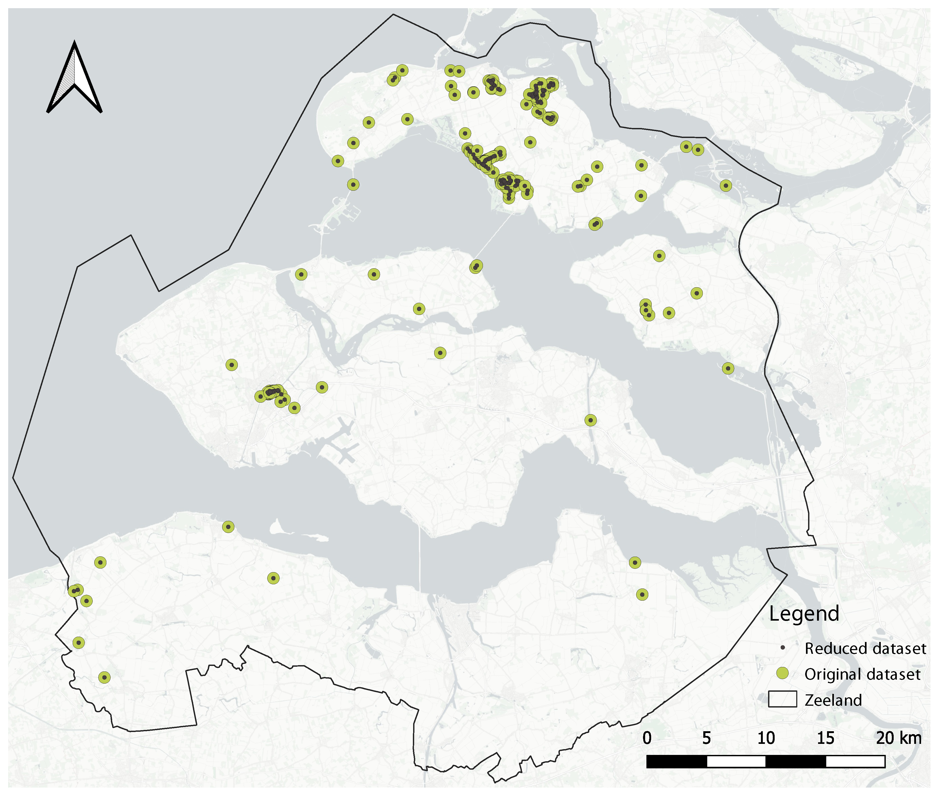
where i = ($x_{i1}$, $x_{i2}$, …, x_in) and j = ($x_{j1}$, $x_{j2}$, …, x_jn) represent two data points described by n numeric attributes. Once DBSCAN is evaluated with the data points of a tourist, for each resulting cluster, its centermost data point is extracted, and the “stay time” feature is updated with the average of “stay time” from the data points in the cluster. This feature will be used during the data-driven characterization stage. This procedure is applied for every (non-filtered) tourist in the dataset to generate a new dataset made of the extracted centermost points.

Then, the Ordering Points To Identify the Clustering Structure (OPTICS) [30] is used to assign cluster membership over the reduced dataset. OPTICS was selected because of its capability to find clusters of varying density. This algorithm uses the same parameters as DBSCAN. However, the only mandatory hyperparameter is the minPts. The search radius (ε) around a data point is optional. It is not fixed and increases while there are not at least minPts data points within which allow OPTICS to identify regions with different density. High density regions will have a small ε while low density regions will have a large ε. Therefore, ε is used to restrict the number of data points considered in the neighborhood search to reduce the computational complexity.

The smallest distance away from a data point that includes minPts other data points is called the core distance (Equation (5)). The distance between a core point p and a core point q within its ε, which cannot be less than the core distance, is the rechability-distance (Equation (5)). The core-distance and reachability-distance were defined in OPTICS [30] as:

$$core\text{-}dis{t}_{ϵ,minPts}(p)=\left\{\begin{array}{cc}UNDEFINED,\hfill & \mathrm{if}Card(N_{ϵ}(p))<minPts\hfill \\ minPts\text{-}dist(p),\hfill & otherwise\hfill \end{array}\right.$$

(4)

$$reachability\text{-}dis{t}_{ϵ,minPts}(p,q)=\left\{\begin{array}{cc}UNDEFINED,\hfill & \mathrm{if}|N_{ϵ}(q))|<minPts\hfill \\ max(core\text{-}dist(q),dist(q,p)),\hfill & otherwise\hfill \end{array}\right.$$

(5)

where minPts-dist(p) is the distance to the minPts nearest neighbor of p, $Card(N_{ϵ}(p))$ is the cardinality of a subset of the dataset D contained in the ε-neighborhood of a data point p, $N_{ϵ}(q)$ is the ε-neighborhood of a data point q, and dist(q,p) is the Euclidean distance between p and q.

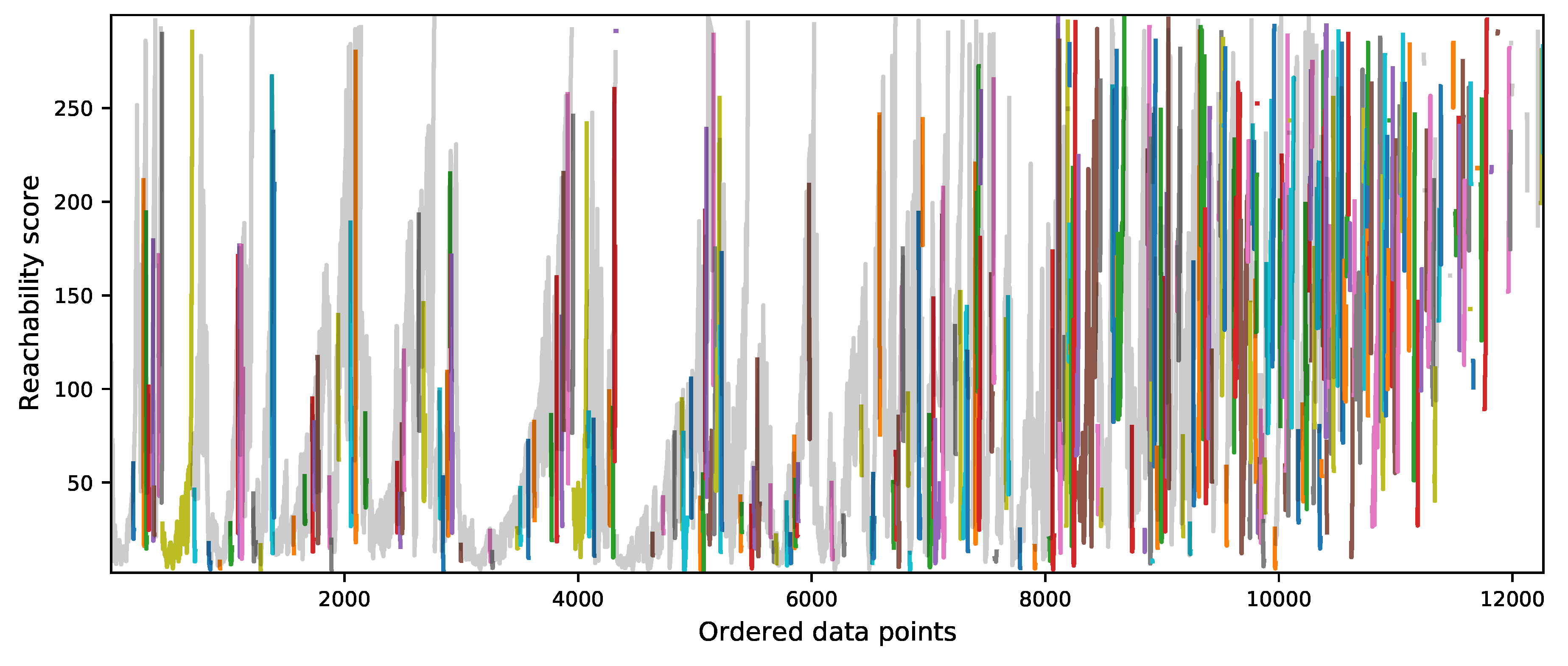
The algorithm starts visiting each data point of the dataset to identify and mark core points. For each point, some computations are performed. First, the core distance and the reachability distance are computed. Second, the reachability score that is defined as the larger of its core distance or its smallest reachability distance is computed. Finally, the sequence of data points that the algorithm is going to visit next is updated based on the reachability distance to the current data point. This means that the next core point to visit is the one with the smallest reachability distance with respect to the current point. Once the algorithm visits all the points, it returns both the order in which each data point was visited and the reachability score of each case.

The clustering extraction process is performed using the Reachability plot. There are two methods to perform the clustering detection. The first method consists of selecting some reachability score to draw a horizontal line across the reachability plot. When the plot dips below the horizontal line, the starting point of a cluster is identified while, if the plot is back above the line, the end of the cluster is identified. Then, any cases above the horizontal line could be classified as noise. The second is the ξ(xi) method which uses the steepness concept defined as 1 − ξ. Here, the start and end of a cluster in the Reachability plot occurs when the reachability of two successive data points change by a factor of 1 − ξ. A downward slope of at least the selected steepness value establishes the start of a cluster while an upward slope of at least the selected steepness value marks its end. In this research, this method is used because of its capabilities to find clusters of different density and also hierarchies among them. However, a clustering algorithm only identifies clusters in the data points, but it does not establish how good or bad they are.

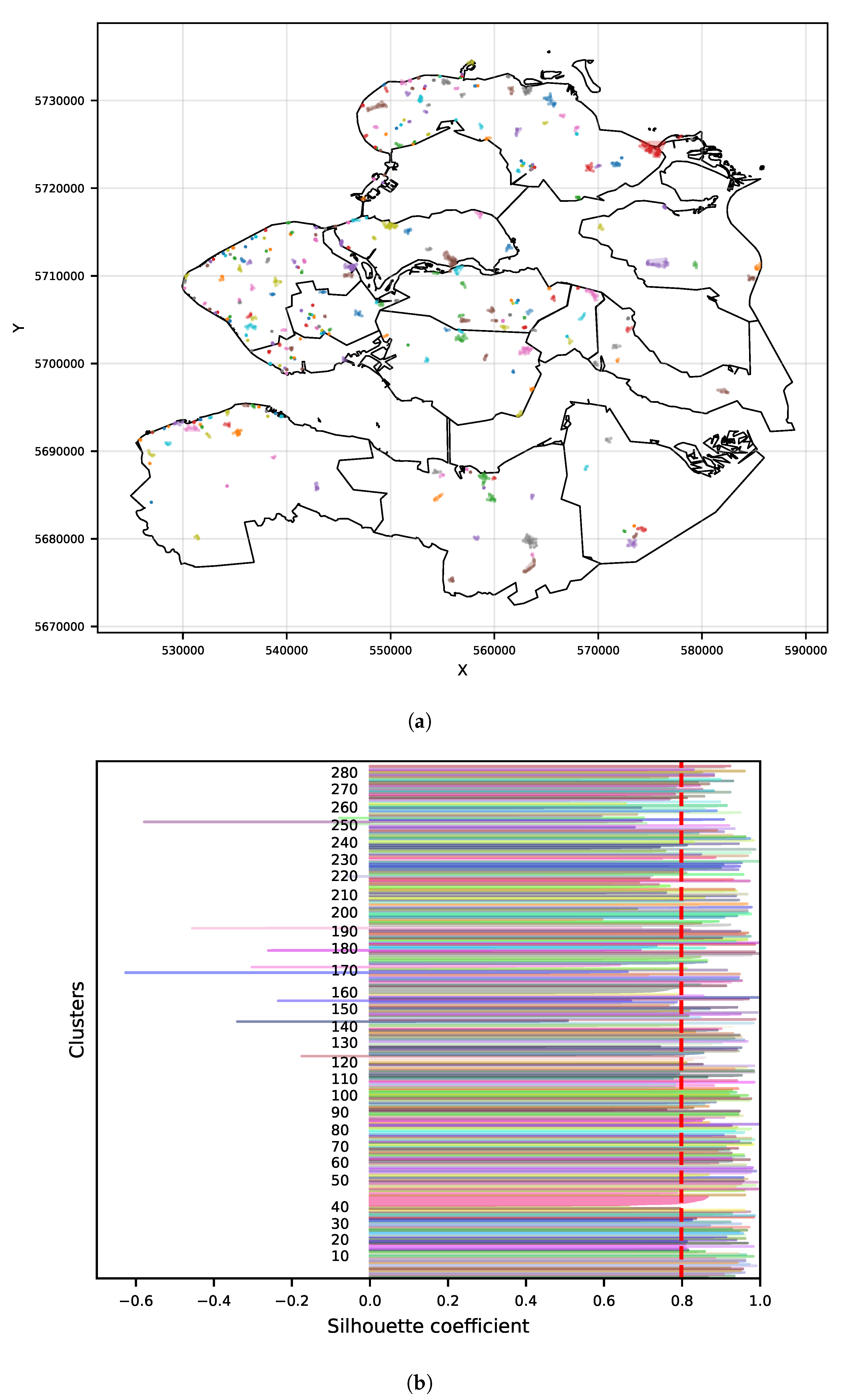
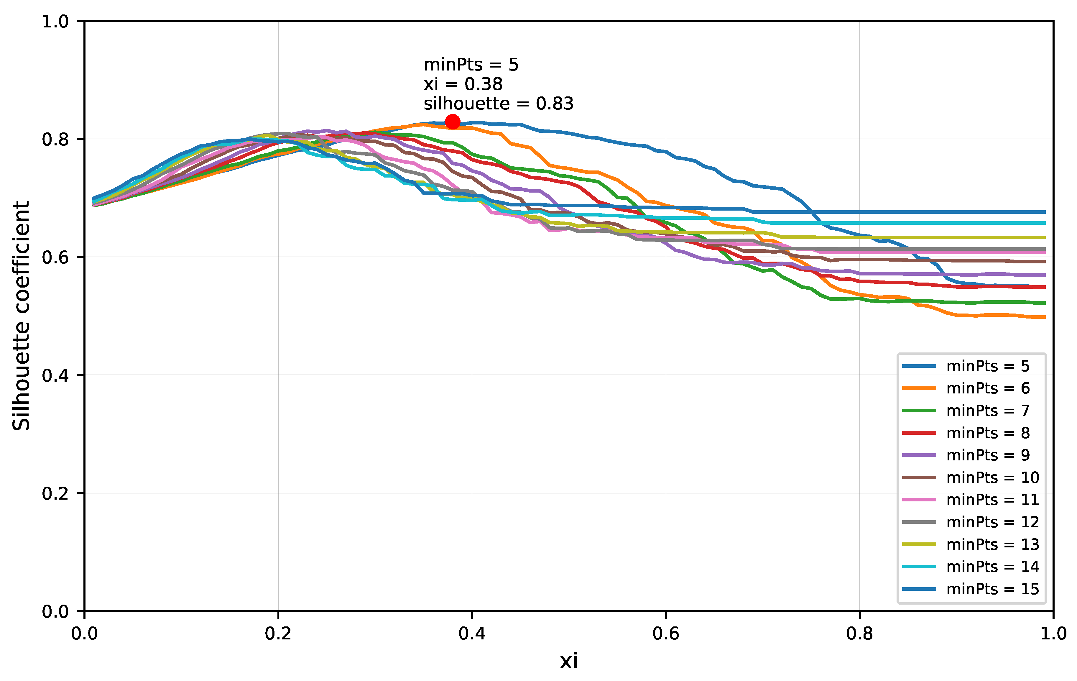
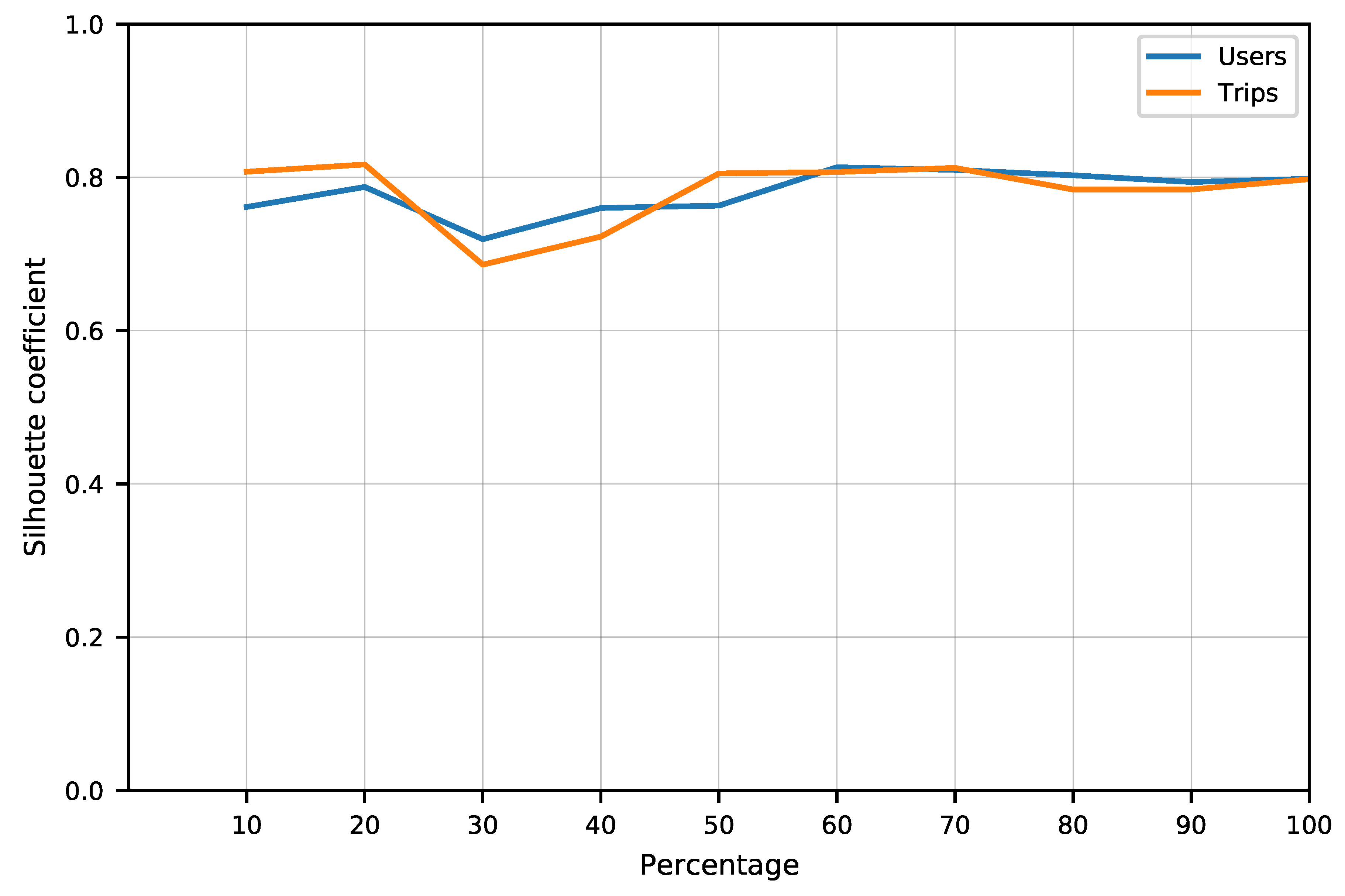
A clustering algorithm computed with different hyperparameters configuration might produce a different clustering result. Therefore, a clustering metric evaluation is used to be able to compare computations of the OPTICS algorithm with different hyperparameter values in order to determine the optimal values where the metric is the best. In this research, the Silhouette Coefficient [38] is used as a metric to evaluate the clustering quality. This metric is used when the ground truth labels are not known. A clustering outcome can be assessed by four criteria: compactness, isolation, global fit, and intrinsic dimensionality [39]. The evaluation of clustering compactness and isolation with this metric is performed for each model generated by each hyperparameter’s combination. The silhouette coefficient is defined as follows:

$$S^{(i)}=\frac{b^{(i)}-a^{(i)}}{max\{b^{(i)},a^{(i)}\}},$$

(6)

where $a^{(i)}$ represents the cluster compactness that is calculated as the average distance between a sample $x^{(i)}$ and all other data points in the same cluster, and $b^{(i)}$ represents the cluster isolation that is calculated as the average distance between the sample $x^{(i)}$ and all samples in the nearest cluster. The Silhouette Coefficient is bounded between –1 for incorrect clustering and +1 for highly dense clustering. Scores around zero indicate overlapping clusters. The experiments for tuning the OPTICS hyperparameters minPts and ξ are described in Section 3.2.

2.3.4. Data-Driven Characterization and Validation

After selecting the optimal hyperparameter values, i.e., the values combination where the average Silhouette Coefficient score among the resulted clusters is the highest, OPTICS is performed using them to produce a clustering model with the more dense and well separated clusters. Then, a data-driven characterization of every cluster (hotspot) is performed. During this stage, the land-use dataset is used and the stay time feature of the cluster data points. The land-use of each data point is established according to the destination location attribute, i.e., a cluster might have data points with different land-use. Then, the main land-use of a cluster is characterized by the most repeated land-use among their data points. Additionally, the average of stay time between the cluster data points to give insights about the time behaviour of the tourists in the cluster is computed.

In the last stage, considering that the land-use is associated with human activities that are developed in a property, the relative number of hotspots by land-use to be compared with the activities of overnight tourists of the area under study described in the validation dataset is calculated. The clustering needs to be performed again with another hyperparameter value if there is no match between these data sources. Otherwise, the clusters (hotspots) will be provided as an outcome of this processing chain.

3. Results

This section presents the results of the analysis to discover hotspots where tourists spend time in the studied region.

3.1. Inbound Travel Analysis for Representativeness

The representativeness of the crowdsourced dataset was evaluated based on its comparison with the statistics of tourist in tourist accommodations data from the Statistics Netherlands. The plot depicted in Figure 4 shows the cumulative distribution functions of the crowdsourced dataset and the official statistics. The K-S distance to determine whether or not both samples come from a population with the same distribution is D = 0.23 and the p-value = 0.90.

The K–S distance for the critical value table with α = 0.05, n = 12 and m = 12 is D-crit = 0.84. Since D = 0.23 < 0.84, there is not a significant difference between the distributions for the samples, which means that both samples come from a population with the same distribution suggesting that the crowdsourced dataset is representative for this study.

3.2. Experiment

A density-based clustering analysis is performed in two stages over the dataset made of 25,613 data points. The first stage aims to reduce the number of data points generated by every individual user in order to prevent after the identification of clusters made by data points from just one user. The procedure starts by extracting n subsets of data points, one for each user, to then apply DBSCAN to each subset.

In the literature, spatial buffer ranges from 20 to 1000 m has been used in different studies to analyze the stationary behavior of a user [40,41,42]. Therefore, the ε hyperparameter value was fixed to 50 m. Then, it is sought to represent the multiple visits made by a user to the same place with one single data point while places visited just once have to be kept. Based on these two premises, minPts = 1 is selected. With this hyperparameter value, non data points will be classified as noise by DBSCAN. Then, we apply DBSCAN on every subset to perform the data compression by user. In cases where a cluster is made of more than one data point, the center most data point is taken to represent the cluster. The resulting dataset contains 12,337 data points, 48.17% from the original dataset. Figure 5 shows the comparison between the original data and the compress data of a user.

The next step consists of applying OPTICS to discover clusters in the already compressed dataset. In the experiment, the ε hyperparameter value is set to reduce the computational complexity. A suitable value was selected by plotting the points’ k-NN distance (Figure 6) in increasing order to look for a knee in the plot. Then, k = 3 is used based on the number of features of the dataset plus one. A distance of ε = 300 m was selected as the maximum search radius around a data point. In other words, the algorithm search in a data point will stop when the core distance reaches 300 m.

The hyperparameter value section can not be done from the data. The minPts and xi hyperparameters are tuned looking for the optimal value combination to execute the OPTICS algorithm with the dataset and to perform the clustering selection based on different densities. First, the hyperparameter search space is defined. The minPts hyperparameter is bounded between 5 and 15 for the minimum and maximum number of points that a data point should have in its neighborhood to be a cluster. It increases in steps of one data point. The xi hyperparameter is bounded between 0 and 1, in steps of 0.01. Second, using a bootstrapping approach, 10 samples are generated from 70% of the dataset, stratified by municipality and tourist segment. Then, for each bootstrap sample, the OPTICS algorithm is computed with ${minPts}_i$, and using each ${xi}_j$ to extract the clusters. The average Silhouette Coefficient (Equation (6)) is computed to measure the goodness of the clustering result using ${minPts}_i$ at ${xi}_j$. Finally, the average of the quality metric among the bootstrap samples for each combination of hyperparameters values is performed. Figure 7 shows how the Silhouette Coefficient changes for each combination of minPts and xi. Here, every curve represents the average Silhouette Coefficient among the 10 bootstrap samples.

Finally, the minPts and xi values are selected where the average Silhouette Coefficient score is highest. This is visible in Figure 7 at 0.83. Therefore, the model with the more dense and well separated clusters is the one with minPts = 5 and xi = 0.38. Then, the OPTICS algorithm is applied on the complete dataset using minPts = 5. A steepness value of xi = 0.38 is used to extract clusters with different densities. The reachability plot for this clustering model is shown in Figure 8.

The clustering model computed with the selected values identifies 288 clusters into the dataset. The location of these clusters is shown in Figure 9a. The Silhouette Coefficient for each of the resulting clusters was computed to explore the quality of every cluster. Figure 9b shows that 11 clusters have a negative Silhouette Coefficient while the rest have a score greater than 0, which represents a good cluster result. The average Silhouette Coefficient of the 288 clusters is 0.79.

3.3. Tourist Hotspot Data-Driven Insights

In this work, there is no application ground truth data to explicitly determine whether or not the resulting clusters match with the statistics of tourist behaviour. However, the land-use dataset from The Netherlands is used to give a data-driven interpretation to characterize the clusters (hotspots) that were identified. The land-use is assigned for each data point of the dataset, so a hotspot might have more than one land-use. Then, the main land-use of every hotspot was assigned based on the most repeated land-use among their data points.

Table 6. Number of hotspots by the most likely land-use.

Level 1	Area (%)	Level 2	Hotspots
Agriculture	36.85	Other agricultural use	17
Airport	0.01	Airport	1
Built	2.21	Allotment	1
		Residential area	68
		Retail and catering	26
		Socio-cultural provision	3
Business premises	1.02	Business premises	23
Dry natural terrain	1.04	Dry natural terrain	49
Forest	1.11	Forest	3
Highway	1.78	Highway	24
Recreation	1.31	Day recreation area	9
		Leisure recreation	36
		Park and public garden	3
		Sports field	5
Semi-built	1.01	Building site	4
		Cemetery	1
		Semi-paved other terrain	13
Water	49.77	Estuary	1
Wet natural terrain	1.86	Wet natural terrain	1

shows the number of identified hotspots by land-use.

According to the CVO 2015 dataset, tourists mainly visit the area for outdoor recreation such as a beach visit. This matches with the results in Section 3.2. It is identified that 35.42% of the hotspots are related with recreational activities, 18.40% of them have a Recreational land-use while the remaining 17.01% are on Dry natural terrain areas that include beaches. Results indicate that the second main group of hotspots (9.03%) is located in Retail and Catering areas, matching with the second most activity undertaken during holidays recorded in CVO 2015. Finally, the third most common land-use in the dataset (7.99%) is Business Premises.

In this study, the behaviour of two tourist segments of the tourist market from the Province of Zeeland is analysed. Figure 10 shows the identified hotspots by tourist segment. Results indicate that both tourist segments are present in most of the hotspots; however, it is noticed that the recurring visitors also explore places far from the coastline.

In order to gain insights about the timing behaviour of tourists in the hotspots, for each hotspot, the average staying time using the data points that are made was computed. Figure 11 shows the hotspot distribution by tourist staying time. Results show that 51% of the hotspots are related to places where the tourist stays less than 4 h.

The timing behaviour of tourists by the location of the hotspot is shown in Figure 12. Results reveal that the occurrence of hotspots, where the tourists stay more than 4 h, is more often in the mainland than on the coast.

3.4. Crowdsourced Tourist Campaign Insights

Tourism crowdsourced campaigns allow us to understand visitors’ behavior, to know where they come from, and their preferred arrival times to the study area. Those insights are important to establish policies for positioning different attractive destinations, sustainable tourism activities, and improving visitor experiences [1].

Figure 13 shows the distribution of hours in which tourists arrive at the study area. It is observed that the External long tourist segment has an arrival time around noon, presenting the same pattern during weekdays and weekends. This figure also reveals that the arrival time of the External recurring tourist segment is distributed during the whole day and concentrated around 2 in the afternoon which matches check-in in most of the accommodation places.

In order to gain a better insight about the number of tourists in a tourism crowdsourced campaign against the quality of the resulting clustering, a deeper analysis at how the average Silhouette Coefficient changes according to the available number of tourists was done. The OPTICS algorithm was computed using the selected hyperparameter values on subsets varying the number of tourists in 10%. Figure 14 shows how this quality metric varies for each case. The Silhouette Coefficient becomes more stable after using data points generated by the 60% (430 users) of the available tourist from the dataset because of increased density of the data points in the discovered hotspots.

4. Discussion

Using tourism crowdsourced data to support tourist managers implies using a chain of processes to transform the raw data into knowledge as the proposed methodology. Before performing any analysis, crowdsourced data needs to be cleaned to handle data quality issues such as missing data, noise, and errors as in any knowledge discovery process [18]. However, solving data quality issues does not guarantee the accuracy, objectivity, and representativeness of crowdsourced data [43,44].

This study contributes to the knowledge about assessing data representativeness of tourism Volunteered Geographic Information sources to provide insight for tourism managers. Different methods have been used to assess the data representativeness to ensure the usefulness of the results from a public policy perspective [45]. In [46], they aimed to mine user-generated and crowdsourced content from the participants, so they applied a survey to ensure that participants were representative of the overall U.S. Internet population. To assess different representativeness aspects of crowdsourced mobility data, in [44], a validation process with criteria such as geographic coverage, origin–destination match, demographic match, distance–duration distributions, and route match is proposed. In this study, the evaluation of representativeness of tourism crowdsourced data from two segments of the tourist marked is performed through the use of a external datasource such as the tourism official statistics as shown in Section 3.1. It was proved that both datasets come from a population with the same distribution suggesting that the crowdsourced dataset is representative for this study. However, it does not guarantee that the crowdsourced dataset is not biased due to the collection method [47]. This is a limitation of the method because of the lack of socio-economic and psychographic descriptors, but this dataset is still a valuable source of information due to the level of detail available.

Then, a tourism data analysis was performed combining density-based clustering approaches to get favourable outcomes in the search of spots where the tourism activities from a specific segment of a tourist market take place. In this paper, data collected from 1505 app users, which recorded 124,725 trips and 151,612 trip segments was used. In addition, 12,337 stationary data points were identified. Such data are used as input for a geo-spatial analysis utilizing clustering techniques to detect hotspots where the tourism activities of External long and External recurring tourist segments are carried out. In addition, 288 clusters (hotspots) were identified. Based on the analysis of the hotspots’ main land-use related with trip purpose, three large groups stand out. Representing 35.42% of the total of hotspots, the largest group is associated with recreational places. It is made of 102 hotspots, 53 of them have a “Recreational” land-use, and 49 have a “Dry natural terrain” land-use to which beaches belong. The second group represents 9.03%, 26 of the total hotspots, and it is associated with “Retail and catering” as the main land-use. Finally, the hotspots associated with “Business premises” represent 7.99%.

The hotspot land-use analysis reveals a high similarity between the most common trip purpose documented by the official statistics from the Province of Zeeland with these mobile crowdsourced discovered hotspots. The main trip purpose to visit the area is for recreation [48]. The areas where the land-use is “Recreational” or “Dry natural terrain” represents only 2.35% of the Province of Zeeland. The largest group of hotspots identified has a land-use where recreational activities are developed suggesting that the smartphone data have the potential to successfully represent the tourism hotspots in a given area as well as to provide more longitudinal insights into tourism related activity behaviour.

In order to explore the tourist behaviour, detailed insights are provided about the hotspots. First, the clusters were characterized based on the tourist segments present on them. Results show that 65 clusters are made of only External recuring tourists, while six clusters are made of only External long tourists. Therefore, both tourist segments are present in most of the clusters; however, it was noticed that the recurring visitors are more present in spots far from the coastline. Then, the clusters were characterized based on the average staying time of the tourist in a hotspot. Results show a tourist stays between 1 and 4 h in 51% of the hotspots identified.

The lack of ground truth activity-related data of the visitor can be seen as a potential limitation in the proposed methodology. This might be tackled by implementing a 2-channel functionality to provide feedback about the main activity that the tourist is doing when a stationary time is sensed. Another potential limitation is related with the smartphone sensed data quality. The proposed method identifies that 8.33% of the clusters have “Highway” as land-use. Due to the noise present in this type of data, weights based on the geography location accuracy and land-use of the data points when assigning the main land-use of a cluster might be considered. However, the geographical location accuracy is not available in the mobile sensed dataset.

Following this, the future lines of research will be focused on the definition of a clustering evaluation metric that considers also contextual information such as the land-use during the evaluation analysis.

5. Conclusions

This research describes a methodology that contributes to the knowledge about assessing data representativeness of tourism Volunteered Geographical Information sources. It also uses density-based clustering techniques to discover potential hotspots from smartphone sensed data. Using crowdsourced data collected by a tourism application such as Zeeland App, the applicability of the method for supporting tourist managers with insights that this type of data can bring on top of the existing statistic and the characterization the tourist behavior of segments from the tourist market is shown. The design, parameter tuning, execution, and results performing the method have also been presented. There were identified 288 clusters (hotspots). According to the land-use, three main groups are identified: 102 hotspots (35.42%) related with a recreational land-use, 26 hotspots (9.03%) with a “Retail and catering” land-use, and 23 hotspots (7.99%) associated with “Business premises”. The obtained results indicate a potential use of smartphone sensed data as a complementary method to traditional tourism surveys when activity-related behaviour insights are required from a large geographic area. However, the tourist managers still need to take care of the usual data-driven pitfalls such as a correct representation of the population [49] and results that depend on positional/temporal accuracy and the errors introduced by the processing [50]. Thus, several questions still remain for future research and these are mainly focused on the integration of different data sources and insights in order for reliable conclusions for policy support to come.

References

1. OECD. OECD Tourism Trends and Policies 2020; OECD Publishing: Paris, France, 2020. [Google Scholar] [CrossRef]
2. Tkaczynski, A.; Rundle-Thiele, S.R.; Beaumont, N. Segmentation: A tourism stakeholder view. Tour. Manag. 2009, 30, 169–175. [Google Scholar] [CrossRef] [Green Version]
3. Bloom, J.Z. MARKET SEGMENTATION: A Neural Network Application. Ann. Tour. Res. 2005, 32, 93–111. [Google Scholar] [CrossRef]
4. Hardy, A.; Hyslop, S.; Booth, K.; Robards, B.; Aryal, J.; Gretzel, U.; Eccleston, R. Tracking tourists’ travel with smartphone-based GPS technology: A methodological discussion. Inf. Technol. Tour. 2017, 17, 255–274. [Google Scholar] [CrossRef]
5. Kellner, L.; Egger, R. Tracking tourist spatial-temporal behavior in urban places, a methodological overview and GPS case study. In Information and Communication Technologies in Tourism 2016; Springer: Cham, Switzerland, 2016; pp. 481–494. [Google Scholar]
6. Frochot, I. A benefit segmentation of tourists in rural areas: A Scottish perspective. Tour. Manag. 2005, 26, 335–346. [Google Scholar] [CrossRef]
7. Hu, B.; Yu, H. Segmentation by craft selection criteria and shopping involvement. Tour. Manag. 2007, 28, 1079–1092. [Google Scholar] [CrossRef]
8. Ahas, R.; Aasa, A.; Mark, Ü.; Pae, T.; Kull, A. Seasonal tourism spaces in Estonia: Case study with mobile positioning data. Tour. Manag. 2007, 28, 898–910. [Google Scholar] [CrossRef]
9. Rodríguez, J.; Semanjski, I.; Gautama, S.; Van de Weghe, N.; Ochoa, D.; Rodríguez, J.; Semanjski, I.; Gautama, S.; Van de Weghe, N.; Ochoa, D. Unsupervised Hierarchical Clustering Approach for Tourism Market Segmentation Based on Crowdsourced Mobile Phone Data. Sensors 2018, 18, 2972. [Google Scholar] [CrossRef] [Green Version]
10. Michail, A.; Gavalas, D. Bucketfood: A Crowdsourcing Platform for Promoting Gastronomic Tourism. In Proceedings of the 2019 IEEE International Conference on Pervasive Computing and Communications Workshops (PerCom Workshops), Kyoto, Japan, 11–15 March 2019; pp. 9–14. [Google Scholar]
11. Download Zeeland App—VVV Zeeland. Available online: https://www.vvvzeeland.nl/en/service/zeeland-app/ (accessed on 5 October 2020).
12. Ahas, R.; Aasa, A.; Roose, A.; Mark, Ü.; Silm, S. Evaluating passive mobile positioning data for tourism surveys: An Estonian case study. Tour. Manag. 2008, 29, 469–486. [Google Scholar] [CrossRef]
13. Yang, C.; Clarke, K.; Shekhar, S.; Tao, C.V. Big Spatiotemporal Data Analytics: A research and innovation frontier. Int. J. Geogr. Inf. Sci. 2019, 34, 1075–1088. [Google Scholar] [CrossRef] [Green Version]
14. Wu, C.; Yang, Z.; Xu, Y.; Zhao, Y.; Liu, Y. Human mobility enhances global positioning accuracy for mobile phone localization. IEEE Trans. Parallel Distrib. Syst. 2014, 26, 131–141. [Google Scholar] [CrossRef]
15. Spangenberg, T. Development of a mobile toolkit to support research on human mobility behavior using GPS trajectories. Inf. Technol. Tour. 2014, 14, 317–346. [Google Scholar] [CrossRef]
16. Semanjski, I.; Bellens, R.; Gautama, S.; Witlox, F. Integrating big data into a sustainable mobility policy 2.0 planning support system. Sustainability 2016, 8, 1142. [Google Scholar] [CrossRef] [Green Version]
17. González, M.C.; Hidalgo, C.A.; Barabási, A.L. Understanding individual human mobility patterns. Nature 2008, 453, 779–782. [Google Scholar] [CrossRef] [PubMed]
18. Fayyad, U.; Piatetsky-Shapiro, G.; Smyth, P. From data mining to knowledge discovery in databases. AI Mag. 1996, 17, 37–53. [Google Scholar]
19. Versichele, M.; de Groote, L.; Claeys Bouuaert, M.; Neutens, T.; Moerman, I.; Van de Weghe, N. Pattern mining in tourist attraction visits through association rule learning on Bluetooth tracking data: A case study of Ghent, Belgium. Tour. Manag. 2014, 44, 67–81. [Google Scholar] [CrossRef] [Green Version]
20. Semanjski, I.; Ramachi, M.; Gautama, S. Detection of Points of Interest from Crowdsourced Tourism Data. In Computational Science and Its Applications–ICCSA 2019; Misra, S., Gervasi, O., Murgante, B., Stankova, E., Korkhov, V., Torre, C., Rocha, A.M.A., Taniar, D., Apduhan, B.O., Tarantino, E., Eds.; Springer International Publishing: Cham, Switzerland, 2019; pp. 203–216. [Google Scholar]
21. Tang, L.; Gao, J.; Ren, C.; Zhang, X.; Yang, X.; Kan, Z. Detecting and Evaluating Urban Clusters with Spatiotemporal Big Data. Sensors 2019, 19, 461. [Google Scholar] [CrossRef] [Green Version]
22. Atiencia, Y.; Cruz, E.; Vaca, C.; Zambrano, L. Spatio-temporal Analysis: Using Instagram Posts to Characterize Urban Point-of-interest. In Proceedings of the 2020 Seventh International Conference on eDemocracy eGovernment (ICEDEG), Buenos Aires, Argentina, 22–24 April 2020; pp. 114–119. [Google Scholar]
23. Trendrapport Toerisme, Recreatie en Vrije Tijd. 2019. Available online: https://www.cbs.nl/nl-nl/publicatie/2019/48/trendrapport-toerisme-recreatie-en-vrije-tijd-2019 (accessed on 10 September 2020).
24. Centraal Bureau Voor de Statistiek—StatLine—Overnight Accommodation; Guests, Country of Residence, Type, Region. Available online: https://opendata.cbs.nl/#/CBS/en/dataset/82059ENG/table (accessed on 8 July 2020).
25. Dataset: CBS Bestand Bodemgebruik. 2015. Available online: https://www.pdok.nl/introductie/-/article/cbs-bestand-bodemgebruik (accessed on 10 September 2020).
26. De Customer Journey Cycle in Zeeland. Available online: https://kwaliteit.toerismevlaanderen.be/de-customer-journey-cycle-in-zeeland (accessed on 10 September 2020).
27. Rhys, H.I. Machine Learning with R, the Tidyverse, and mlr, 1st ed.; Manning Publications Co.: Shelter Island, NY, USA, 2020; p. 536. [Google Scholar]
28. Ester, M.; Kriegel, H.P.; Sander, J.; Xu, X. A density-based algorithm for discovering clusters in large spatial databases with noise. In Proceedings of the Second International Conference on Knowledge Discovery and Data Mining, Portland, OR, USA, 2–4 August 1996; pp. 226–231. [Google Scholar]
29. Zhou, A.; Zhou, S.; Cao, J.; Fan, Y.; Hu, Y. Approaches for scaling DBSCAN algorithm to large spatial databases. J. Comput. Sci. Technol. 2000, 15, 509–526. [Google Scholar] [CrossRef]
30. Ankerst, M.; Breunig, M.M.; Kriegel, H.P.; Sander, J. OPTICS: Ordering Points to Identify the Clustering Structure. SIGMOD Rec. (ACM Spec. Interest Group Manag. Data) 1999, 28, 49–60. [Google Scholar] [CrossRef]
31. Bryant, A.; Cios, K. RNN-DBSCAN: A Density-Based Clustering Algorithm Using Reverse Nearest Neighbor Density Estimates. IEEE Trans. Knowl. Data Eng. 2018, 30, 1109–1121. [Google Scholar] [CrossRef]
32. Kisilevich, S.; Mansmann, F.; Keim, D. P-DBSCAN: A density based clustering algorithm for exploration and analysis of attractive areas using collections of geo-tagged photos. In Proceedings of the 1st International Conference and Exhibition on Computing for Geospatial research & Application, Washington, DC, USA, 21–23 June 2010; pp. 1–4. [Google Scholar]
33. Schubert, E.; Sander, J.; Ester, M.; Kriegel, H.P.; Xu, X. DBSCAN Revisited, Revisited: Why and How You Should (Still) Use DBSCAN. ACM Trans. Database Syst. 2017, 42. [Google Scholar] [CrossRef]
34. Hu, Y.; Gao, S.; Janowicz, K.; Yu, B.; Li, W.; Prasad, S. Extracting and understanding urban areas of interest using geotagged photos. Comput. Environ. Urban Syst. 2015, 54, 240–254. [Google Scholar] [CrossRef]
35. Birant, D.; Kut, A. ST-DBSCAN: An algorithm for clustering spatial–temporal data. Data Knowl. Eng. 2007, 60, 208–221. [Google Scholar] [CrossRef]
36. Devkota, B.; Miyazaki, H.; Witayangkurn, A.; Kim, S.M. Using Volunteered Geographic Information and Nighttime Light Remote Sensing Data to Identify Tourism Areas of Interest. Sustainability 2019, 11, 4718. [Google Scholar] [CrossRef] [Green Version]
37. Vu, H.Q.; Li, G.; Law, R.; Ye, B.H. Exploring the travel behaviors of inbound tourists to Hong Kong using geotagged photos. Tour. Manag. 2015, 46, 222–232. [Google Scholar] [CrossRef]
38. Rousseeuw, P.J. Silhouettes: A graphical aid to the interpretation and validation of cluster analysis. J. Comput. Appl. Math. 1987, 20, 53–65. [Google Scholar] [CrossRef] [Green Version]
39. Dubes, R.; Jain, A.K. Validity studies in clustering methodologies. Pattern Recognit. 1979, 11, 235–254. [Google Scholar] [CrossRef]
40. Rodríguez Echeverría, J.; Gautama, S.; Van de Weghe, N.; Ochoa, D.; Ortiz Jaramillo, B. Efficient use of geographical information systems for improving transport mode classification. In DATA ANALYTICS 2018: The Seventh International Conference on Data Analytics, Athens, Greece, 18–22 November 2018; Bhulai, S., Kardaras, D., Semanjski, I., Eds.; International Academy, Research and Industry Association (IARIA): Wilmington, DE, USA, 2018; pp. 130–135. [Google Scholar]
41. Filip Biljecki, H.L.; van Oosterom, P. Transportation Mode-based Segmentation and Classification of Movement Trajectories. Int. J. Geogr. Inf. Sci. 2013, 27, 385–407. [Google Scholar] [CrossRef]
42. Gong, H.; Chen, C.; Bialostozky, E.; Lawson, C.T. A GPS/GIS method for travel mode detection in New York City. Comput. Environ. Urban Syst. 2012, 36, 131–139. [Google Scholar] [CrossRef]
43. Basiri, A.; Haklay, M.; Foody, G.; Mooney, P. Crowdsourced geospatial data quality: Challenges and future directions. Int. J. Geogr. Inf. Sci. 2019, 33, 1588–1593. [Google Scholar] [CrossRef] [Green Version]
44. Leao, S.Z.; Lieske, S.N.; Pettit, C.J. Validating crowdsourced bicycling mobility data for supporting city planning. Transp. Lett. 2019, 11, 486–497. [Google Scholar] [CrossRef]
45. Bubalo, M.; van Zanten, B.T.; Verburg, P.H. Crowdsourcing geo-information on landscape perceptions and preferences: A review. Landsc. Urban Plan. 2019, 184, 101–111. [Google Scholar] [CrossRef]
46. Ghose, A.; Ipeirotis, P.G.; Li, B. Designing ranking systems for hotels on travel search engines by mining user-generated and crowdsourced content. Mark. Sci. 2012, 31, 493–520. [Google Scholar] [CrossRef] [Green Version]
47. Yuan, Y.; Wei, G.; Lu, Y. Evaluating gender representativeness of location-based social media: A case study of Weibo. Ann. GIS 2018, 24, 163–176. [Google Scholar] [CrossRef]
48. Omvang Toerisme in Zeeland 2018—Projectenportfolio. Available online: https://www.projectenportfolio.nl/wiki/index.php/KCKT_Publication_PR_00006 (accessed on 8 July 2020).
49. Weinberg, J.D.; Freese, J.; McElhattan, D. Comparing Data Characteristics and Results of an Online Factorial Survey between a Population-Based and a Crowdsource-Recruited Sample. Sociol. Sci. 2014, 1, 292–310. [Google Scholar] [CrossRef]
50. Van Gheluwe, C.; Lopez, A.J.; Gautama, S. Error sources in the analysis of crowdsourced spatial tracking data. In Proceedings of the 2019 IEEE International Conference on Pervasive Computing and Communications Workshops (PerCom Workshops), Kyoto, Japan, 11–15 March 2019; pp. 183–188. [Google Scholar]
Figure 1. Province of Zeeland, The Netherlands.
Ijgi 09 00686 g001
Figure 2. Methodology steps.
Ijgi 09 00686 g002
Figure 3. Trip’s destination locations in the Province of Zeeland.
Ijgi 09 00686 g003
Figure 4. CBS vs. Zeeland app data distribution comparison.
Ijgi 09 00686 g004
Figure 5. Dataset compression for one user: 466 data points were down to 178 points, representing 61.80% compression.
Ijgi 09 00686 g005
Figure 6. K-NN distance using k = 3.
Ijgi 09 00686 g006
Figure 7. Tuning of minPts and xi parameters.
Ijgi 09 00686 g007
Figure 8. Reachability plot.
Ijgi 09 00686 g008
Figure 9. Silhouette analysis for OPTICS clustering model with minPts = 5 and xi = 0.38. (a) Visualization of the 288 resulting cluster in the study area. (b) Silhouette plot of the 288 clusters.
Ijgi 09 00686 g009
Figure 10. Hotspot locations by tourist segment.
Ijgi 09 00686 g010
Figure 11. Number of clusters by number of staying hours.
Ijgi 09 00686 g011
Figure 12. Hotspots by staying time: (a) less than 2 h; (b) between 2 and 4 h; (c) between 4 and 6 h; (d) more than 6 h.
Ijgi 09 00686 g012
Figure 13. Distribution of hourly arrivals of inbound trips during the study period. (a) external long tourist segment; (b) external recurring tourist segment.
Ijgi 09 00686 g013
Figure 14. Average Silhouette Coefficient for clustering model with different number of users in the study area.
Ijgi 09 00686 g014