A Theoretical Approach for Forecasting Different Types of Drought Simultaneously, Using Entropy Theory and Machine-Learning Methods

Abstract

Precipitation deficit can affect different natural resources such as water, soil, rivers and plants, and cause meteorological, hydrological and agricultural droughts. Multivariate drought indexes can theoretically show the severity and weakness of various drought types simultaneously. This study introduces an approach for forecasting joint deficit index (JDI) and multivariate standardized precipitation index (MSPI) by using machine–learning methods and entropy theory. JDI and MSPI were calculated for the 1–12 months’ time window (JDI_1–12 and MSPI_1–12), using monthly precipitation data. The methods implemented for forecasting are group method of data handling (GMDH), generalized regression neural network (GRNN), least squared support vector machine (LSSVM), adaptive neuro-fuzzy inference system (ANFIS) and ANFIS optimized with three heuristic optimization algorithms, differential evolution (DE), genetic algorithm (GA) and particle swarm optimization (PSO) as meta-innovative methods (ANFIS-DE, ANFIS-GA and ANFIS-PSO). Monthly precipitation, monthly temperature and previous amounts of the index’s values were used as inputs to the models. Data from 10 synoptic stations situated in the widest climatic zone of Iran (extra arid-cold climate) were employed. Optimal model inputs were selected by gamma test and entropy theory. The evaluation results, which were given using mean absolute error (MAE), root mean squared error (RMSE) and Willmott index (WI), show that the machine learning and meta-innovative models can present acceptable forecasts of general drought’s conditions. The algorithms DE, GA and PSO, could improve the ANFIS’s performance by 39.4%, 38.7% and 22.6%, respectively. Among all the applied models, the GMDH shows the best forecasting accuracy with MAE = 0.280, RMSE = 0.374 and WI = 0.955. In addition, the models could forecast MSPI better than JDI in the majority of cases (stations). Among the two methods used to select the optimal inputs, it is difficult to select one as a better input selector, but according to the results, more attention can be paid to entropy theory in drought studies.

1. Introduction

Drought forecasting is one of the major concerns to the water managers, agriculturalists and other water exploiters. Iran, especially its central desert, is situated on the arid and extra-arid belt of the world and the drought intensity variations directly influence the people’s life, agriculture, surface water and groundwater in the country. During the years 1998–2000, Iran experienced one of the worst and the costliest drought periods that occurred in the last 50 years. During this three-year dry period, water scarcity reached a crisis point in more than 270 cities, thousands of villages ran out of drinking water, the rate of surface water flow decreased to 55%, and Iran’s dam and reservoirs have had to operate at their minimum volume capacity to transfer water because of the low inflows and high temperatures [1,2]. Thus, the investigation of the meteorological, hydrological and agricultural droughts is of great importance to the country. Drought indices can show the weakness and intensity of different types of droughts separately, but in recent years, certain indices have been introduced for indicating the intensity and weakness of the various types of droughts together, in a single series [3]. Among the most important of these indices, the multivariate standard precipitation index (MSPI) and joint deficit index (JDI) can be pointed out. These indices combine some series of standard precipitation indices (SPI) that each of them indicates a certain type of drought [4]. The combination is based on the various statistical methods, and the result reflects the general status of the drought in a given month.

JDI was first introduced by Kao and Govindaraju [5] as a joint drought index. They introduced the modified standard precipitation index (SPImod) in a study and pooled 1–12 month time window to come up with JDI and asserted that the method could be implemented on all of the other hydrological variables, such as the discharge rates of the rivers plus the precipitation data. After that, Mirabbasi et al. [6] calculated JDI for 50 rain gauges in the north of Iran during the period from 1970 to 2007. They concluded that JDI could provide a comprehensive view of the short- and long-term status of the drought in Iran, and they also forecasted rainfall for one to three-month horizons to investigate the drought status by JDI for the forthcoming months. In a study, Hao and Singh [7] investigated the multivariate indices of drought, including JDI, and the applied characteristics and weak and strong points of these indices. Ma et al. [8] combined JDI and standardized Palmer Index to introduce SPDI-JDI (standardized Palmer drought index-based joint drought index) index for ten climatic zones in Texas.

In 2014, Bazrafshan et al. [9] introduced the MSPI index as a joint drought index. They examined SPI’s time windows by performing principal component analysis and applied them to four stations from various climates in Iran and showed that the first principal component (PC1) could account for 74% of the general drought variations. Bazrafshan et al. [2] have investigated MSPI and JDI in terms of multivariate drought monitoring for 42 meteorological stations all over Iran. They calculated both of the indices for 1–12 month time window (which monitors meteorological, hydrological and agricultural droughts simultaneously) and showed that MSPI outperforms JDI for illustrating the intensity and weakness of drought in Iran’s climates. Bateni et al. [10] used MSPI for introducing the agrometeorological drought indices (AMDI-SA). In addition, MSPI prediction has been reported for Iranian climates in Aghelpour et al. [11] study for agricultural drought forecasting.

Since the droughts begin slowly, it is possible to rely on real-time predictions so that measures can be taken and policies can be adopted for reducing the drought effects [12]. In recent years, many models have been employed for predicting the drought indices, amongst which machine learning-based models can be pointed out. Moreover, metaheuristic models are obtained by blending these models with optimization algorithms that are applied to predicting drought. These models have been widely used for predicting the SPI family, such as SPI as the meteorological drought index [13,14,15,16] and SPEI as the agricultural drought index [17,18,19,20,21], and their favorable performance has been reported under various climatic conditions. For example, Kisi et al. [22] used adaptive neuro-fuzzy inference system (ANFIS) and its hybrid forms with particle swarm optimization (PSO) and genetic algorithm (GA) for forecasting SPI as a meteorological drought index. Malik et al. used [23] a co-active neuro-fuzzy inference system (CANFIS) for forecasting streamflow drought index (SDI), which is a hydrological drought index of the SPI family. Soh et al. [17] used the wavelet ANFIS model and SPEI indicator for forecasting agricultural drought. In most of the drought studies, machine learning models had significantly acceptable performances in predicting different types of droughts separately.

According to the research done, however, no model has been evaluated to forecast different types of droughts simultaneously, as well as the selection of optimal model inputs is a challenge for nonlinear dynamic models. The questions as to which inputs should be used for model development have been a challenge in practice. Although much research has been done on drought forecasting issues, most of them do not consider effective input selection for drought modeling. As a result, the main challenge lies in the evaluation of existing data and assessing the adequacy of data. Although modeling improves performance by adding information, observations show that adding information improves model performance only slightly. Modeling accuracy can be reduced by increasing information. This is because additional information causes the model to be over-fitted. The over-fitted model also performs well in training but has a very poor performance in testing. Overfitting also occurs when multivariate models have too much input data. It is, therefore, important to know which inputs are effective in modeling and which are not [24,25,26,27]. Furthermore, MSPI has been forecasted by ANFIS and its hybrid-type models [11], but it has been investigated just from the perspective of agricultural drought. In fact, the present study is the first research trying to forecast multivariate drought in extra-arid climates, based on the indices JDI and MSPI; which can theoretically show the severity and weakness of meteorological, hydrological and agricultural droughts, simultaneously. Thus, the current research paper is intended to evaluate the performance of machine learning and metaheuristic models for forecasting these two multivariate drought indices. Furthermore, as another innovation in drought forecasting studies, entropy theory and gamma tests have been used for selecting the suitable predictor input variables.

2. Materials and Methods

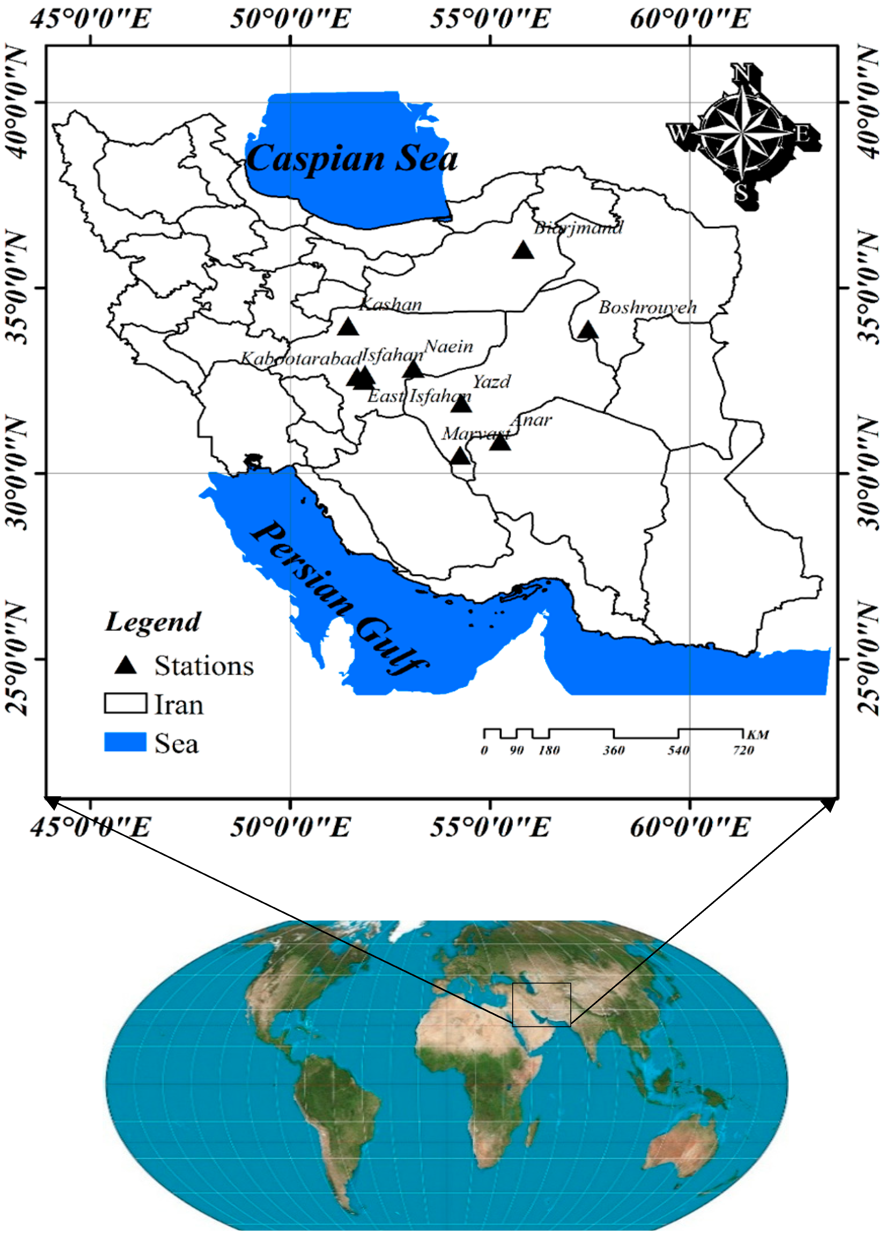
2.1. Study Region

Based on the extended De Marton Climatic Zones Classification Method, the widest climatic class of Iran is the extra-arid cold climatic zone. This zone has an area of 352,738.4 km² in Iran, which accounts for about 21.4% of the country’s total area [28]. Based on this method, ten synoptic stations are specified in this climactic breadth, as shown in Figure 1. In the present study, drought monitoring and prediction are carried out in these ten stations. The reason for choosing this climate is that drought’s damaging effects are more significant in extra arid areas.

The information used in this study includes monthly precipitation (P) and temperature (T) data whose positions and statistical specifications have been summarized in

Table 1. Synoptic stations’ position and data specification.

Station	X	Y	Z	Period	Mean		St. Dev. (a)		Max. (b)		Min. (c)		Skew. (d)		Annual Mean
					P (e) (mm)	T (f) (°C)	P (mm)	T (°C)	P (mm)	T (°C)	P (mm)	T (°C)	P (mm)	T (°C)	P (mm)	T (°C)
Anar	30.88	55.25	1408.80	1986–2017	5.88	20.32	10.69	8.93	92.10	35.50	0.00	0.70	2.86	−0.08	70.56	20.32
Biarjmand	36.05	55.83	1106.20	1992–2017	10.14	16.36	13.77	9.71	85.30	32.10	0.00	−4.40	2.48	−0.11	121.68	16.36
Boshrouyeh	33.90	57.45	885.00	1988–2017	7.17	21.09	11.39	10.33	78.70	36.60	0.00	−5.80	2.21	−0.15	86.04	21.09
East Isfahan	32.67	51.87	1543.00	1980–2017	8.44	15.42	12.56	9.55	86.00	31.70	0.00	−2.60	2.20	−0.03	101.28	15.42
Isfahan	32.62	51.67	1550.40	1951–2017	10.41	16.45	15.59	9.26	148.20	32.00	0.00	−3.40	2.51	−0.05	124.92	16.45
Kabootarabad	32.52	51.85	1545.00	1992–2017	9.41	17.93	13.54	9.58	69.00	33.20	0.00	−2.10	1.81	−0.04	112.92	17.93
Kashan	33.98	51.45	982.30	1967–2017	11.10	19.82	16.38	10.29	124.10	37.50	0.00	−5.10	2.51	−0.08	133.20	19.82
Marvast	30.50	54.25	1546.60	1997–2017	5.34	19.85	10.14	8.93	64.80	34.20	0.00	3.60	2.69	−0.03	64.08	19.85
Naein	32.85	53.08	1549.00	1993–2017	7.87	18.66	12.44	9.35	85.60	34.30	0.00	−3.40	2.55	−0.10	94.44	18.66
Yazd	31.90	54.28	1237.20	1953–2017	4.72	19.59	8.76	9.56	69.20	36.10	0.00	−1.10	3.11	−0.08	56.64	19.59

^(a) St. Dev. = standard deviation; ^(b) Max. = maximum; ^(c) Min. = minimum; ^(d) Skew. = skewness; ^(e) P = precipitation; ^(f) T = temperature.

. As observed from the table, precipitation data have skewed distribution (skewness ranges from 1.81 (Kabootarabad) to 3.11 (Yazd)). The data of each of these stations were procured from the general office of the country’s meteorology organization for the period of time from their establishment years till 2017. The precipitation data have been utilized for calculating both of the indices, i.e., JDI and MSPI, and also used as input to the prediction models. The monthly temperature data were also used as input, and their effects on the models’ accuracy were also investigated.

2.2. Indices

2.2.1. Joint Deficit Index (JDI)

The index was designed for the investigation of the joint behavior of the precipitation in SPImod’s 1-month to 12-month time windows considering their seasonal changes and combines the time windows of SPImod, as one time window of JDI (JDI_1–12). JDI is essentially based on Copula Functions. This index uses a 12-dimensional experimental copula for showing the associations between SPImod’s time windows [5]. The experimental copula is based on the empirical ranking scales of joint experimental likelihood. For example, the 12D experimental copula is computed by Equation (1) for an n-numbered sample:

$$C_n\left(u_1.\dots .u_{12}\right)=\frac{1}{n}{\displaystyle \sum }_{i=1}^{n}I\left(\frac{R_{i1}}{n+1}\le u_1.\dots .\frac{R_{i12}}{n+1}\le u_{12}\right)$$

(1)

where I (A) denotes the logical A term that is assigned a value equal to unity in case of holding true and zero in the otherwise case. (R_i1, …, R_i12) are the ranks of the observed ith datum that are, respectively, shown as u₁, …, u₁₂. For more information, please refer to Kao and Govindaraju [5].

2.2.2. Multivariate Standardized Precipitation Index

The index is capable of blending several SPI variables, each of which belongs to a time window in one single series. The method that was used by Bazrafshan et al. [9] for this blending is principal component analysis (PCA). By this method, a large part of the drought intensity variability in different time windows is summarized in 1 series [9]. MSPI is based on the first principal component (PC1) that is a linear combination of k-time windows capable of explaining the highest percentage of variability in k first variables. The notable point is that their values cannot be compared between various places and months due to the algebraic properties of PC1, meaning that, unlike SPI that takes a mean value between 0 and 1, PC1 lacks such a trait, and hence, it must be standardized in respect to the mean and standard deviation of the various months (Equation (2)):

$$Z_{1ym}=\frac{P{C}_{1ym}-\overline{P{C}_{1m}}}{S{D}_{1m}}\approx \frac{P{C}_{1ym}}{S{D}_{1m}}$$

(2)

In this equation, Z_1ym is the standardized value of PC1 in yth year and mth month; $\overline{P{C}_{1m}}$ is the mean value of PC1 in mth month, and SD_1m is the standard deviation of PC1 in the mth month. Here, Z_1ym is the value of MSPI. For more information regarding the MSPI calculation method, please refer to the original article by Bazrafshan et al. [9]. The drought intensity categories of these two indices are like SPI, as presented in

Table 2. Classification of the SPI’s values and corresponding probability limits [9,29].

SPI Classes	Probability Limits	Description
SPI ≥ 2	≥97%	Extremely wet
2 > SPI ≥ 1.5	93.3–97.7%	Severely wet
1.5 > SPI ≥ 1	84.1–93.3%	Moderately wet
1 > SPI > −1	15.9–84.1%	Normal
−1 ≥ SPI > −1.5	6.7–15.9%	Moderately dry
−1.5 ≥ SPI > −2	2.3–6.7%	Severely dry
−2 ≥ SPI	2.3% ≥	Extremely dry

:

Since JDI is calculated for 1–12 months’ time window (JDI_1–12), MSPI has also been calculated for the same time window (MSPI_1–12). Moreover, because 1-month SPI (SPI₁) indicates the drought status from meteorological perspectives, 3-month SPI (SPI₃) shows drought status from soil moisture viewpoint, 6-month SPI (SPI₆) reflects hydrological drought conditions (river streams and dam reservoirs), and 9-month to 12-month SPIs (SPI₉, SPI₁₀, SPI₁₁ and SPI₁₂) can express the agricultural drought status [4], so the 1–12 month time window can concomitantly exhibit all the meteorological, soil moisture, hydrological and agricultural drought conditions, together. In the current research paper, these two indices (JDI and MSPI) were calculated using MATLAB Software.

2.3. Input Determination Methods

After calculating the indices and before prediction by the models, two methods of entropy theory and gamma test were utilized for selecting the optimal inputs and accelerating the modeling task. These methods are described below.

2.3.1. Gamma Test

Gamma test shows the variance of the estimated error according to the direct data. Thus, the error estimation that is commonly termed gamma test can be considered as equivalent to the sum of nonlinear error squares [30]. To have a better understanding of the gamma test in case of assuming that two points x and x’ approaching one another in the input space corresponding to y and y’ as outputs, these two points should also be approaching one another in the output space, otherwise the non-approaching of these two points stems from the difference caused by errors (noises) [31].

2.3.2. Entropy Theory

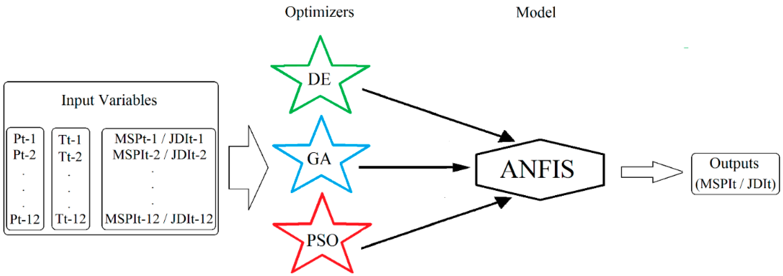
Shannon proposed the main concept of information theory in 1948 [32]. The definition of entropy is derived from information theory that analyzes a series of statistical structures from numerical series, signs and symbols establishing relationships between the signals [33]. In general, four types of entropy were introduced for quantifying the information content: boundary entropy, joint entropy, conditional entropy and information transfer entropy. The present study uses information transfer entropy that is succinctly explained as follows:

Shannon specified the first boundary entropy, named H(x), from a discrete random variable, x:

$$H\left(x\right)=-K{\displaystyle \sum }_{i=1}^{n}P\left(x_i\right)logP\left(x_i\right)$$

(3)

The parameter takes a value equal to unity (K = 1) on the condition that the amount of H(x) logarithm is expressed based on Napier’s constant (e); n expresses the number of events with a probability of $P\left(x_i\right)=\left(i=1.2.\dots .n\right)$.

The entropy of two random and independent variables of x and y is obtained from the sum of the boundary entropy of the two variables:

$$H\left(x.y\right)=H\left(x\right)+H\left(y\right)$$

(4)

When the two random variables of x and y are associated, the joint entropy takes a value smaller than the total entropy obtained from Equation (5):

$$T\left(x.y\right)=H\left(x\right)+H\left(y\right)-H\left(x.y\right)$$

(5)

Information transfer entropy is another type of entropy specifying the mutual relationship between x and y, and it is obtained as the differential of the total and joint entropies for the two dependent variables x and y [34]:

$$T\left(x.y\right)=H\left(x\right)-H\left(x|y\right)=H\left(y\right)-H\left(x|y\right)$$

(6)

Here, H(x|y) expresses the conditional entropy. The conditional entropy indicates x if y expresses the residual uncertainty in x on the condition that y is clearly known and vice versa.

According to the above explanations, entropy calculations can be generalized to M variables. The total entropy for the independent variable, $x_m\left(m=1.2.\dots .M\right)$, is computable from Equation (7):

$$H\left(x_1.x_2.\dots .x_M\right)={\displaystyle \sum }_{m=1}^{M}H\left(x_m\right)$$

(7)

If the variables are associated, their joint entropy is calculated from Equation (8):

$$H\left(x_1.x_2.\dots .x_M\right)=H\left(x_1\right)+{\displaystyle \sum }_{m=1}^{M}H\left(x_m|x_1.x_2.\dots .x_{m-1}\right)$$

(8)

The complementary information for entropy theory can be found in [27].

2.4. Models

2.4.1. Adaptive Neuro-Fuzzy Inference System (ANFIS)

ANFIS is a model that uses neural network learning algorithms and fuzzy logic for designing nonlinear maps between the input and output spaces. The model is capable of learning by neural networks and defining and using the relationships between input–output variables by fuzzy rules, and subsequently creating the input structure of the system.

Three methods of grid partitioning, subtractive clustering and fuzzy c-means are utilized in the classical ANFIS model, and the present study uses fuzzy c-means [35]. For more information about the details of the ANFIS model and fuzzy c-means method, the reference to articles by Jang et al. [36] is suggested.

In the present study, three strong optimization algorithms have also been used for optimizing the ANFIS model, as briefly explained below.

2.4.2. Differential Evolution (DE) Algorithm

This algorithm is a method in the area of complementary calculations, and it was introduced by Storn and Price [32]. DE begins working by providing a series of suggested responses and tries to find the optimum response within a series of consecutive iterations. The most important feature of this algorithm is its high speed, simplicity and strength. DE sets three primary parameters of population size (NP), mutation weight (F) and crossing (Cr). For more information, please see the articles presented by Storn and Price [37] and Halabi et al. [38].

2.4.3. Genetic Algorithm (GA)

This algorithm was introduced by Holland [39]. The principal component in GA is a chromosome that is consisted of genes, and each gene explains a parameter of the problem [40]. As the most important stage in the genetic algorithm, the selection is the process through which the next generation’s chromosomes are determined based on the current generation’s survival law. In this algorithm, the search is commenced in an initial population of the strains and the unique strains are evaluated in each repetition corresponding to an efficiency condition and assigned a proportion value. For complementary information, refer to the article by Jaramillo et al. [41].

2.4.4. Particle Swarm Optimization (PSO) Algorithm

PSO was inspired by the collective movement of the fish or birds’ flight in groups [42], and it was subsequently employed successfully in various sciences. In this algorithm, each solution is just a particle in the search space [43]. All of the particles are assigned a fitness value evaluated by a fitness function that must be optimized. Further information on the PSO algorithm can be found in Eberhart and Kennedy [42].

The schematic form of the ANFIS model, as well as its combination with DE, GA and PSO algorithms, is illustrated in Figure 2, considering the studied inputs and outputs. In this prediction approach, the time lags of each index can only be used to predict the same index; so here, this procedure is used for predicting JDI and MSPI separately.

2.4.5. Group Method of Data Handling (GMDH)

This model was offered in 1970 by Ivakhnenko, and it is a multivariate nonlinear statistical analysis [39]. GMDH is based on the ability to distinguish nested second- or third-degree polynomials for simulating regression and performing classification. In GMDH, each composite layer is comprised of several nodes as the model’s inputs for the transfer function. The results are transferred to the next layer that is per se employed as an input layer for the next layer of the network [40]. For more information, refer to articles by Ivakhnenko [44], Aghelpour and Varshavian [45], Ashrafzadeh et al. [46] and Aghelpour et al. [47]

2.4.6. Generalized Regression Neural Network (GRNN)

This type of neural network is one type of multipurpose basic and approximating radial neural networks for smooth functions. GRNN is a three-layer neural network in which, like the other neural networks [48]. The number of neurons existent on the first and last layers is, respectively, equal to the dimensions of the input and output vectors, but, unlike the other networks, the number of the neurons in the hidden layer of GRNN is equal to the number of the observed data. This type of neural network uses normal efficiency function in each of the neurons of the hidden layer, and the data inputted into this function for each neuron include the Euclidean distance between the input and observed data related to that neuron. See the sources for complementary information on GRNN [45,48,49].

2.4.7. Least Squares Support Vector Machine (LSSVM)

The least-squares support vector machine (LSSVM) was proposed by Suykens and Vandewalle in 1999, and it is used for the prediction of the turbulent time series [50]. LSSVM is a type of support vector machine that uses a collection of linear equations for training, while SVM uses a second-degree optimization problem, and this is their major difference [51]. For complementary information about this model, refer to Moazenzadeh and Mohammadi [52], Mohammadi and Aghashariatmadri [53] and Guan et al. [54].

2.5. Performance Evaluation Scales

To ensure the accuracy of the models’ predictions, mean absolute error (MAE), root mean square error (RMSE), Willmott index (WI) and Pearson’s correlation coefficient (R) were employed, and their related equations are shown in Equations (9)–(12):

$$\mathrm{MAE}=\frac{1}{\mathrm{n}}{\displaystyle \sum }_{\mathrm{i}=1}^{\mathrm{n}}\left|{\mathrm{y}}_{\mathrm{i}}-{\mathrm{f}}_{\mathrm{i}}\right|$$

(9)

$$\mathrm{RMSE}=\sqrt{\frac{1}{\mathrm{n}}{\displaystyle \sum }_{\mathrm{i}=1}^{\mathrm{n}}{\left({\mathrm{y}}_{\mathrm{i}}-{\mathrm{f}}_{\mathrm{i}}\right)}^2}$$

(10)

$$\mathrm{WI}=1-\frac{{{\displaystyle \sum }}_{\mathrm{i}=1}^{\mathrm{N}}{\left({\mathrm{y}}_{\mathrm{i}}-{\mathrm{f}}_{\mathrm{i}}\right)}^2}{{{\displaystyle \sum }}_{\mathrm{i}=1}^{\mathrm{N}}{\left(\left|{\mathrm{f}}_{\mathrm{i}}-\overline{\mathrm{y}}\right|+\left|{\mathrm{y}}_{\mathrm{i}}-\overline{\mathrm{y}}\right|\right)}^2}$$

(11)

$$\mathrm{R}=\frac{{{\displaystyle \sum }}_{\mathrm{i}=1}^{\mathrm{n}}\left({\mathrm{y}}_{\mathrm{i}}-\overline{\mathrm{y}}\right)\left({\mathrm{f}}_{\mathrm{i}}-\overline{\mathrm{f}}\right)}{\sqrt{{{\displaystyle \sum }}_{\mathrm{i}=1}^{\mathrm{n}}{\left({\mathrm{y}}_{\mathrm{i}}-\overline{\mathrm{y}}\right)}^2}\ast \sqrt{{{\displaystyle \sum }}_{\mathrm{i}=1}^{\mathrm{n}}{\left({\mathrm{f}}_{\mathrm{i}}-\overline{\mathrm{f}}\right)}^2}}$$

(12)

where ${\mathrm{y}}_{\mathrm{i}}$ and $\overline{\mathrm{y}}$ are, respectively the observed data and their means; ${\mathrm{f}}_{\mathrm{i}}$ and $\overline{\mathrm{f}}$ are the model-predicted data and their means, and n is the number of the data.

3. Results

3.1. Input Selection

At first, the models’ inputs, including temperature, precipitation and the values of the index itself, were backwardly arranged up to 12 steps. Since the periodicity of a hydrological process has a 1 year (12 months) return period, it is logical to consider up to 12-month time lags as inputs. Then, gamma tests and entropy theory were utilized for selecting the optimal inputs. The results of these evaluations are given in

Table 3. Chosen inputs by gamma test (●) and entropy theory (∆) for joint deficit index (JDI).

Station	Variable	Time Lags (i)
		1	2	3	4	5	6	7	8	9	10	11	12
Anar	P(a)t-i	●∆	∆	●∆	●∆	●∆	●∆	●∆		∆	●		●∆
	T(b)t-i	∆	●∆	●	●∆	●∆	●∆	●∆	●∆	●∆	●∆	∆	●∆
	JDIt-i	●∆	●∆	●∆	●∆	●∆	●∆	●∆	●∆	●∆	●∆	●∆	●∆
Biarjmand	Pt-i	●∆		●∆	∆	●∆	∆		∆	∆	∆		∆
	Tt-i	●∆	∆	∆	∆	●∆	∆	●∆	●∆	●∆	●∆	∆	∆
	JDIt-i	∆	●∆	∆	●∆	∆	∆	●∆	●∆	∆	∆	∆	∆
Boshrouyeh	Pt-i	●∆	●∆	●∆	∆			∆		●∆		●∆	●
	Tt-i		●	∆	∆	∆	∆	∆	∆			∆
	JDIt-i	∆	∆	∆	∆	∆	∆	∆	∆	∆	∆	∆	∆
East of Isfahan	Pt-i	●∆	●∆	●	∆	∆	∆	∆	●∆	●	∆		●∆
	Tt-i	●∆	●∆	●∆	●∆	●∆	∆	●∆	∆	●∆	●∆	●∆
	JDIt-i	●∆	∆	∆	∆	∆	●∆	●∆	∆	●∆	●∆	●∆	●∆
Isfahan	Pt-i	●∆	●∆	●∆	●∆	●∆	●∆	●∆	●∆	●∆	●∆	●∆
	Tt-i	●∆	∆	∆	∆	∆	∆	∆	●∆	∆	●∆	∆	∆
	JDIt-i	●∆	●∆	●∆	●∆	●∆	●∆	●∆	●∆	●∆	●∆	●∆	∆
Kabootarabad	Pt-i	●∆	∆	●	∆	∆	●∆	∆	●∆	●∆	∆
	Tt-i	∆	●∆	●∆	●∆	●	●	●∆	●∆	●∆	●∆	●∆	●∆
	JDIt-i	∆	∆	●∆	●∆	●∆	∆	∆	∆	●∆	∆	∆	●∆
Kashan	Pt-i	∆	●∆	●∆	∆			∆	∆	●∆		●∆	●∆
	Tt-i	∆	∆	∆	∆	∆	∆	∆	∆	∆	∆	∆	●∆
	JDIt-i	●∆	●∆	●∆	∆	∆	∆	∆	∆	●∆	●∆	∆	●∆
Marvast	Pt-i	●∆	●∆	●∆	●∆	●∆	●				●	●∆
	Tt-i	●∆	●∆	∆	∆	∆	●	●∆	●∆	●∆	∆	∆	∆
	JDIt-i	●∆	●∆	●∆	●∆	●∆	∆	∆	●∆	●∆	●∆	●∆	●∆
Naein	Pt-i	●∆	∆	●∆	●∆	●∆	●∆		●∆	●∆	●∆	●∆	●∆
	Tt-i	∆	∆	∆	∆	∆	∆	∆	∆		∆		∆
	JDIt-i	∆	∆	∆	∆	∆	∆	∆	∆	∆	∆	∆	∆
Yazd	Pt-i	●∆	●∆	●∆	∆	●∆	∆	●∆		∆	∆	∆	●∆
	Tt-i	●∆	∆	●∆	●∆	●∆	●∆	●∆	●∆	●∆	●∆	●∆	●∆
	JDIt-i	∆	●∆	∆	∆	●∆	●∆	●∆	●∆	●∆	●∆	●∆	∆

^(a) P = precipitation; ^(b) T = temperature.

and

Table 4. Chosen inputs by gamma test (●) and entropy theory (∆) for multivariate standardized precipitation index (MSPI).

Station	Variable	Time Lags (i)
		1	2	3	4	5	6	7	8	9	10	11	12
Anar	P(a)t-i	●∆	●∆	●∆	●∆	●∆	●∆	●∆	●∆	●∆	●∆		●∆
	T(b)t-i		∆	●	∆	∆	●∆	●∆	●∆	●∆	●∆	∆
	MSPIt-i	∆	●∆	●∆	●∆	●	●∆	●∆	●	●	●∆	●∆	●
Biarjmand	Pt-i	●∆	●∆	●∆	●∆	●∆	●∆	●∆	●∆	●∆	∆	∆
	Tt-i	●		●∆	∆	●∆	●∆	●	●∆	●∆	●∆	●∆	●
	MSPIt-i	●∆	●∆	∆	●∆	∆	∆	∆	∆	∆	●∆	●∆	●∆
Boshrouyeh	Pt-i	●∆	●∆	●∆	●∆	●∆	●∆	●∆	●∆	●∆	∆	●∆
	Tt-i				●∆		●			●	●∆
	MSPIt-i	●	●∆	∆	●∆	●	●∆	∆	∆	∆	∆	∆
East of Isfahan	Pt-i	●∆	●∆	●∆	●∆	●∆	●∆	●∆	●∆	●∆	∆	●	●
	Tt-i		●∆	●	●	●∆	∆	●∆	●	●	●∆	●	●∆
	MSPIt-i	●∆	●∆	●∆	●∆	●∆	●∆	●∆	●∆	●	∆	∆	∆
Isfahan	Pt-i	●∆	●∆	●∆	●∆	●∆	●∆	●	●∆	●	●	●∆
	Tt-i	●	∆	∆	●∆	∆	∆	∆	∆	●	●∆	∆	∆
	MSPIt-i	●∆	●∆	●∆	●∆	●∆	●∆	●∆	●∆	∆	●∆	●∆	●∆
Kabootarabad	Pt-i	●∆	●∆	●∆	●∆	●∆	●∆	●∆	●∆		∆	●	∆
	Tt-i	●	●	●	●∆	●	●∆	●∆	●	●	●	●∆	●
	MSPIt-i	●∆	●∆	●∆	●∆	●∆	●∆	●∆	●∆	●∆	●∆	●∆	●∆
Kashan	Pt-i	●∆	●∆	●∆	●∆	●∆	●∆	●∆	●∆	●∆	∆	∆	●∆
	Tt-i		∆	∆	∆	∆	∆	∆	∆				∆
	MSPIt-i	∆	∆	∆	∆	∆	∆	∆	∆	∆	∆	∆	∆
Marvast	Pt-i	●∆	●∆	●∆	●∆	●∆	●∆	●∆	●		●	●∆	●
	Tt-i	∆		∆	●	∆	∆	∆	∆	●∆		∆
	MSPIt-i	●∆	●∆	●∆	●∆	●∆	●∆	●∆	●∆	●∆	●∆	●∆	●∆
Naein	Pt-i	●∆	●∆	●∆	●∆	●∆	●∆	∆	●∆	∆	●∆	●∆	●∆
	Tt-i		∆	∆	∆	∆	∆				∆	∆	∆
	MSPIt-i	∆	∆	∆	●∆	●∆	●∆	∆	∆	∆	●∆	∆	∆
Yazd	Pt-i	●∆	●∆	●∆	●∆	●∆	●∆	●∆	∆	●∆		●∆	●∆
	Tt-i	●∆	●∆	●∆	●∆	●∆	●∆	●∆	●	●∆	●∆	●∆	●∆
	MSPIt-i	●∆	∆	●∆	∆	●∆	●∆	●∆	●∆	●∆	●∆	●∆	●∆

^(a) P = precipitation; ^(b) T = temperature.

. In these tables, P and T, respectively, denote the total monthly precipitation and mean temperature. The subscripts t_i, as well, indicate ith time lag for each variable and they were considered as the models’ input in the present study.

In the present study, the processes followed in the article by the references of Ahmadi et al. [18], Biazar et al. [55] and Biazar et al. [56], have also been implemented in such a way that the entropy of the entire data was first calculated in these tables based on the entropy theory and the variables were omitted one-by-one and the entropy values of each combination are calculated in a second stage. If by deleting a variable from the input combination, the entropy value exceeds the primary entropy, the variable should be removed from the input combination. As for the gamma test, the same two stages are executed so that the variable whose gamma value becomes smaller than the initial gamma is removed. This process is separately repeated for all the variables (P, T, JDI and MSPI), and the results of the input selection for JDI and MSPI are summarized in Table 3 and Table 4.

Next, the input and target data (JDIt/MSPIt) are inserted into the models. In the modeling processes of the present study, 75% of the input and target samples was used for training, and 25% of them was applied in testing. In all of the stations, the modeling and prediction of multivariate drought were carried out based on the inputs selected by both of the methods (gamma and entropy). According to the paper’s issue (predicting), in all of the models, the test part was shown in the evaluation tables and discussed.

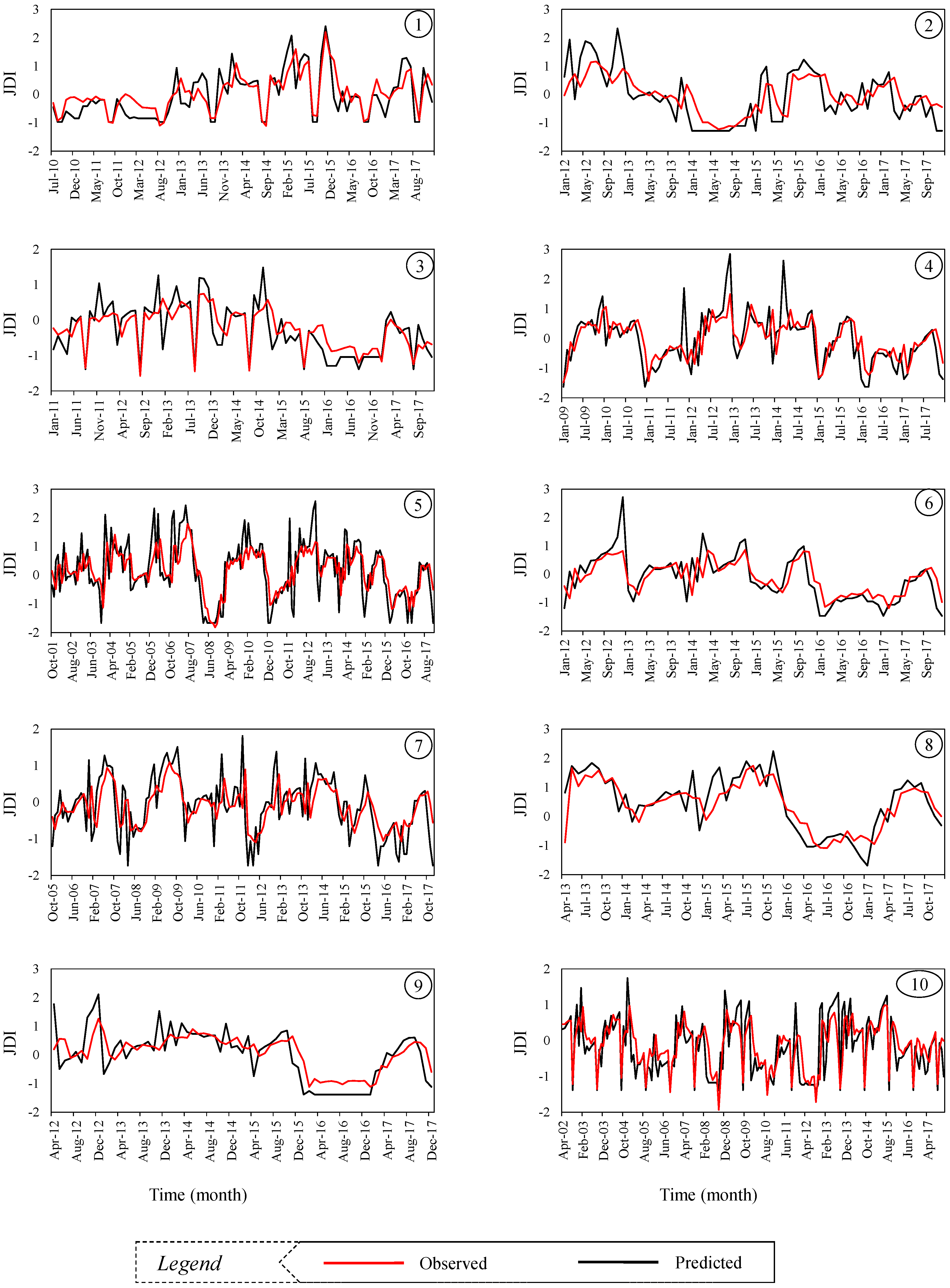
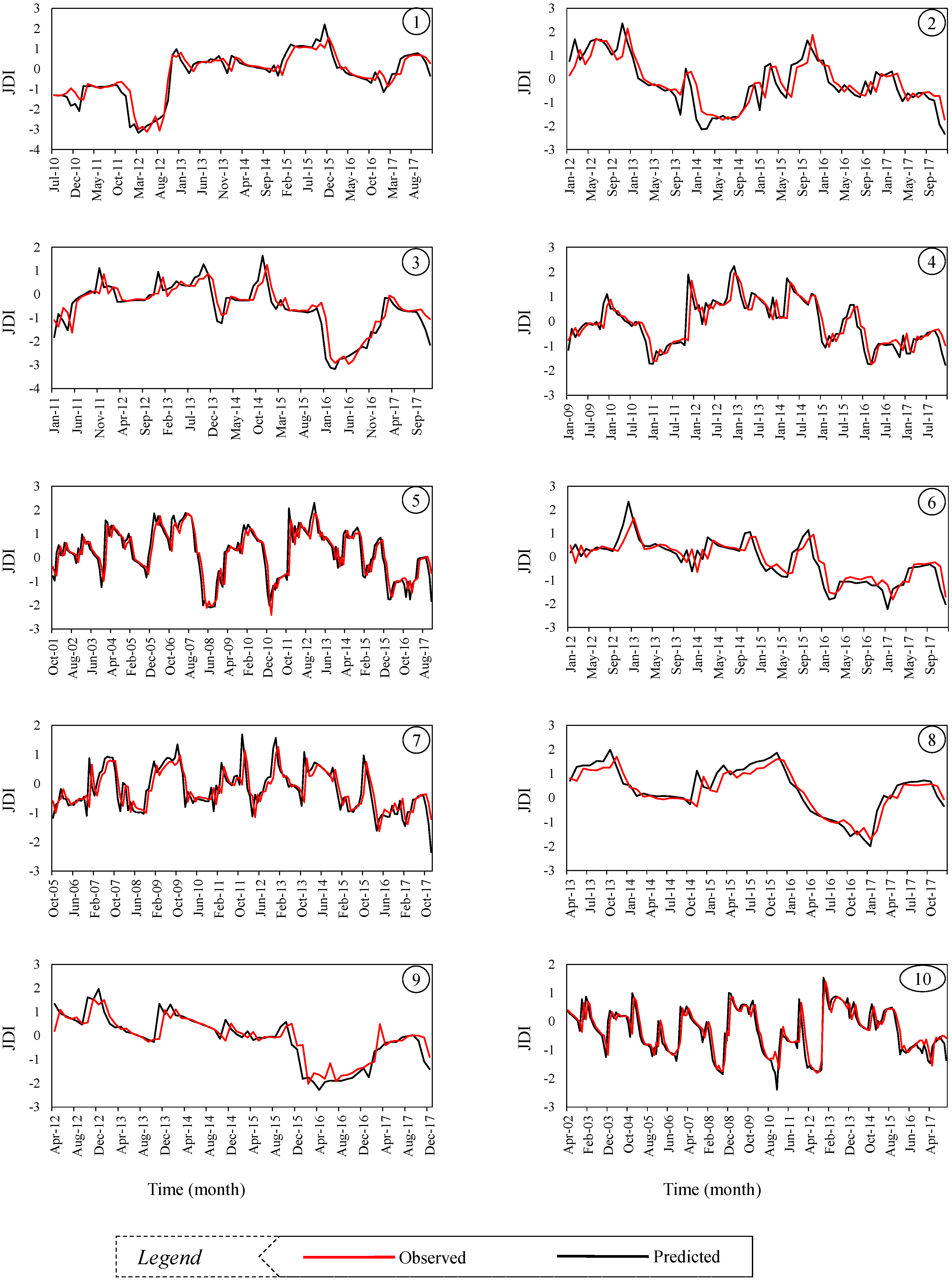
3.2. Results of JDI Prediction

Predicting JDI was implemented by two input scenarios and seven models in 10 stations. The results of JDI prediction are shown in

Table 5. Evaluation criteria for the test period of the models in predicting JDI.

Station	Input Definer	ANFIS			ANFIS-DE			ANFIS-GA			ANFIS-PSO			GMDH			GRNN			LSSVM
		MAE	RMSE	WI	MAE	RMSE	WI	MAE	RMSE	WI	MAE	RMSE	WI	MAE	RMSE	WI	MAE	RMSE	WI	MAE	RMSE	WI
Anar	Gamma	0.562	0.760	0.760	0.525	0.654	0.778	0.543	0.676	0.762	0.576	0.743	0.776	0.415	0.534	0.855	0.559	0.690	0.678	0.461	0.605	0.803
	Entropy	0.576	0.921	0.678	0.512	0.664	0.776	0.513	0.667	0.778	0.503	0.696	0.784	0.398	0.523	0.862	0.544	0.675	0.683	0.468	0.618	0.797
Biarjmand	Gamma	0.673	0.900	0.681	0.591	0.741	0.725	0.574	0.735	0.727	0.610	0.798	0.738	0.543	0.693	0.793	0.710	0.850	0.548	0.615	0.749	0.697
	Entropy	0.682	0.867	0.731	0.582	0.765	0.728	0.575	0.746	0.730	0.624	0.825	0.712	0.531	0.677	0.790	0.750	0.890	0.497	0.607	0.743	0.713
Boshrouyeh	Gamma	0.675	1.166	0.501	0.652	0.802	0.502	0.693	0.818	0.501	0.729	0.871	0.450	0.607	0.722	0.505	0.674	0.818	0.434	0.721	0.850	0.520
	Entropy	0.784	1.149	0.484	0.471	0.593	0.731	0.502	0.642	0.719	0.584	0.749	0.687	0.338	0.456	0.864	0.661	0.777	0.564	0.491	0.644	0.739
East Isfahan	Gamma	0.626	1.207	0.674	0.517	0.723	0.699	0.524	0.737	0.694	0.594	0.826	0.644	0.466	0.653	0.780	0.649	0.851	0.536	0.531	0.731	0.670
	Entropy	0.696	1.198	0.567	0.559	0.758	0.685	0.555	0.747	0.696	0.609	0.815	0.664	0.453	0.645	0.792	0.661	0.824	0.553	0.541	0.734	0.684
Isfahan	Gamma	0.773	0.924	0.770	0.573	0.771	0.788	0.566	0.768	0.784	0.609	0.823	0.764	0.534	0.721	0.803	0.706	0.904	0.630	0.572	0.770	0.777
	Entropy	0.823	1.072	0.696	0.570	0.777	0.786	0.588	0.799	0.782	0.629	0.839	0.756	0.534	0.734	0.794	0.707	0.901	0.618	0.574	0.774	0.772
Kabootarabad	Gamma	0.648	0.887	0.638	0.599	0.770	0.611	0.590	0.764	0.614	0.601	0.808	0.622	0.491	0.656	0.739	0.630	0.746	0.611	0.573	0.740	0.620
	Entropy	0.698	0.854	0.727	0.525	0.684	0.712	0.551	0.724	0.704	0.527	0.706	0.755	0.391	0.555	0.823	0.583	0.733	0.599	0.511	0.669	0.703
Kashan	Gamma	0.604	0.829	0.650	0.489	0.658	0.698	0.486	0.656	0.717	0.521	0.724	0.664	0.440	0.619	0.761	0.634	0.786	0.236	0.474	0.643	0.716
	Entropy	0.652	0.840	0.652	0.491	0.676	0.701	0.495	0.696	0.690	0.574	0.792	0.638	0.455	0.615	0.745	0.585	0.720	0.543	0.490	0.656	0.691
Marvast	Gamma	0.794	1.134	0.702	0.648	0.814	0.785	0.611	0.766	0.805	0.755	0.957	0.712	0.461	0.576	0.884	0.845	1.021	0.598	0.661	0.812	0.711
	Entropy	0.872	1.092	0.699	0.628	0.768	0.782	0.623	0.780	0.783	0.655	0.856	0.749	0.421	0.542	0.899	0.849	1.003	0.615	0.682	0.843	0.689
Naein	Gamma	0.764	0.985	0.669	0.694	0.874	0.533	0.689	0.858	0.539	0.697	0.890	0.599	0.557	0.711	0.732	0.748	0.907	0.469	0.655	0.831	0.620
	Entropy	0.877	0.958	0.615	0.573	0.737	0.734	0.607	0.803	0.679	0.787	1.121	0.507	0.444	0.582	0.837	0.746	0.881	0.368	0.558	0.723	0.706
Yazd	Gamma	0.748	0.815	0.721	0.548	0.689	0.609	0.476	0.615	0.735	0.445	0.595	0.808	0.461	0.611	0.770	0.522	0.657	0.693	0.451	0.601	0.777
	Entropy	0.851	0.724	0.734	0.507	0.651	0.713	0.478	0.627	0.754	0.475	0.628	0.760	0.399	0.551	0.835	0.528	0.669	0.687	0.431	0.578	0.798

The bold numbers are the best performance of each station, on its own row.

.

This includes 140 evaluations for JDI. In these evaluations, there are 70 comparisons between entropy theory and gamma test, which shows the superiority of entropy theory in 43 cases (61.4%). Between the models, GMDH could have the best JDI predictions in all of the stations. The most accurate prediction of JDI is reported for Boshrouyeh station by inputs of entropy theory and GMDH model, with MAE = 0.338, RMSE = 0.456, and WI = 0.864. Among ANFIS and its hybrid models, the bio-inspired algorithms DE, GA and PSO could improve the performance of ANFIS by an average of 32.8%, 32.0% and 20.9%, respectively. The weakest performance belongs to the simple ANFIS model in East Isfahan station, which is given by inputs of gamma test with MAE = 0.626, RMSE = 1.207, and WI = 0.674. The predictions of JDI for each station are shown in time-series plots (Figure 3).

In this figure, the best prediction of each station in the test period (bold cases of Table 5) is presented beside its observation. At the first look at these plots (Figure 3), there is not significant overlapping of the outputs for the stations in JDI prediction. However, in some of the cases, the overlapping can be acceptable. For example, in Boshrouyeh station, the moderate and severe droughts that occurred in Augusts of 2011, 2012, 2013 and 2014, are predicted accurately. Or the moderate drought classes for Yazd station in September of 2002, 2003, 2005, 2007, 2011, 2013, 2014 and 2016, were acceptably predicted. However, in the wet classes of the stations, the overlapping is weak and unacceptable.

3.3. Results of MSPI Prediction

MSPI prediction was also implemented by the inputs of the two aforementioned methods, entropy theory and gamma test, and the evaluation results are shown in

Table 6. Evaluation criteria for the test period of the models in predicting MSPI.

Station	Input Definer	ANFIS			ANFIS-DE			ANFIS-GA			ANFIS-PSO			GMDH			GRNN			LSSVM
		MAE	RMSE	WI	MAE	RMSE	WI	MAE	RMSE	WI	MAE	RMSE	WI	MAE	RMSE	WI	MAE	RMSE	WI	MAE	RMSE	WI
Anar	Gamma	0.582	0.742	0.886	0.466	0.627	0.894	0.487	0.677	0.869	0.530	0.768	0.848	0.381	0.498	0.943	0.671	0.910	0.674	0.574	0.834	0.768
	Entropy	0.596	0.793	0.833	0.417	0.562	0.919	0.434	0.590	0.910	0.562	0.853	0.787	0.271	0.409	0.964	0.668	0.884	0.712	0.510	0.767	0.816
Biarjmand	Gamma	0.684	0.882	0.829	0.467	0.639	0.879	0.474	0.656	0.870	0.584	0.818	0.820	0.420	0.564	0.917	0.699	0.899	0.636	0.481	0.639	0.873
	Entropy	0.694	0.824	0.859	0.487	0.656	0.876	0.501	0.655	0.876	0.570	0.737	0.843	0.398	0.568	0.911	0.731	0.942	0.531	0.487	0.648	0.872
Boshrouyeh	Gamma	1.235	1.086	0.772	0.395	0.535	0.910	0.386	0.528	0.912	0.459	0.649	0.869	0.325	0.476	0.938	0.772	1.068	0.465	0.436	0.600	0.873
	Entropy	1.357	1.080	0.779	0.448	0.609	0.875	0.446	0.606	0.876	0.535	0.821	0.807	0.397	0.571	0.897	0.752	1.042	0.471	0.537	0.734	0.799
East Isfahan	Gamma	0.586	0.905	0.781	0.379	0.552	0.898	0.377	0.549	0.900	0.416	0.615	0.875	0.322	0.498	0.916	0.526	0.701	0.774	0.365	0.530	0.901
	Entropy	0.654	0.881	0.770	0.376	0.563	0.894	0.365	0.539	0.902	0.453	0.648	0.869	0.327	0.499	0.910	0.532	0.674	0.823	0.372	0.541	0.899
Isfahan	Gamma	0.637	0.686	0.879	0.354	0.505	0.929	0.352	0.507	0.929	0.384	0.544	0.919	0.333	0.492	0.932	0.550	0.711	0.829	0.357	0.507	0.928
	Entropy	0.683	0.763	0.864	0.352	0.508	0.928	0.357	0.511	0.928	0.383	0.551	0.915	0.330	0.492	0.935	0.560	0.723	0.821	0.364	0.514	0.924
Kabootarabad	Gamma	0.623	0.776	0.821	0.427	0.575	0.863	0.457	0.639	0.830	0.529	0.790	0.726	0.347	0.474	0.908	0.502	0.704	0.736	0.429	0.596	0.841
	Entropy	0.666	0.665	0.859	0.421	0.573	0.862	0.447	0.577	0.866	0.424	0.552	0.888	0.335	0.454	0.919	0.486	0.677	0.761	0.430	0.591	0.843
Kashan	Gamma	0.707	0.613	0.799	0.434	0.586	0.742	0.432	0.600	0.737	0.456	0.608	0.758	0.479	0.620	0.707	0.452	0.603	0.747	0.425	0.574	0.788
	Entropy	0.588	0.688	0.758	0.347	0.502	0.842	0.342	0.501	0.844	0.380	0.537	0.826	0.326	0.464	0.866	0.425	0.551	0.782	0.333	0.494	0.844
Marvast	Gamma	0.590	0.882	0.783	0.382	0.490	0.916	0.368	0.463	0.924	0.428	0.634	0.877	0.296	0.389	0.951	0.802	0.953	0.633	0.395	0.492	0.910
	Entropy	0.640	0.819	0.796	0.382	0.477	0.920	0.382	0.477	0.920	0.416	0.547	0.908	0.280	0.374	0.955	0.741	0.906	0.680	0.379	0.479	0.913
Naein	Gamma	0.643	0.888	0.805	0.590	0.770	0.770	0.576	0.765	0.775	0.634	0.827	0.761	0.456	0.637	0.855	0.679	0.838	0.668	0.613	0.802	0.743
	Entropy	0.724	0.892	0.767	0.362	0.528	0.910	0.363	0.518	0.915	0.521	0.773	0.829	0.290	0.458	0.938	0.692	0.847	0.651	0.382	0.550	0.897
Yazd	Gamma	0.592	0.666	0.805	0.306	0.462	0.897	0.306	0.462	0.897	0.300	0.502	0.881	0.253	0.389	0.929	0.465	0.603	0.764	0.306	0.458	0.896
	Entropy	0.633	0.627	0.844	0.307	0.463	0.897	0.305	0.461	0.900	0.293	0.460	0.901	0.257	0.419	0.917	0.470	0.610	0.764	0.305	0.458	0.897

The bold numbers are the best performance of each station, on its own row.

.

Similarly, for this index, there are 140 evaluations and 70 comparisons between the input selectors too. In 40 cases (about 57.1%), entropy theory was superior in comparison to gamma tests. In MSPI prediction like JDI, GMDH is evaluated as the most accurate model, which had the best predictions in all of the investigated stations. The most accurate prediction of MSPI with MAE = 0.280, RMSE = 0.374 and WI = 0.955, is made for Marvast station by GMDH model and inputs of entropy theory. In evaluating ANFIS and its hybrid forms, the results showed that DE, GA and PSO algorithms could cause on average 45.9%, 45.4% and 24.2% improvement for ANFIS, respectively. The weakest MSPI prediction is reported for the ANFIS model in Boshrouyeh station, with MAE = 1.235, RMSE = 1.086 and WI = 0.772, which is given by the inputs of gamma tests. In Figure 4, the overlapping of MSPI predictions and their observations are shown in time series plots.

In these graphs, the best predictions of each station (bold cases of Table 5) are drawn. At first look at Figure 4, it is obvious that there is stronger overlapping in MSPI prediction compared to JDI in all of the stations. The predictions of stations East Isfahan, Isfahan, Kashan and Yazd, have significant overlapping with their observations, even in severe and extreme drought events. The weakest MSPI predictions can be reported for Biarjmand and Boshrouyeh stations, but in comparison with JDI, they are significantly more accurate. In addition, in wet classes, the predictions of MSPI are acceptable in all of the investigated stations. In addition, the scatter plots for comparing the predicted, and observed values are provided in Figure 5.

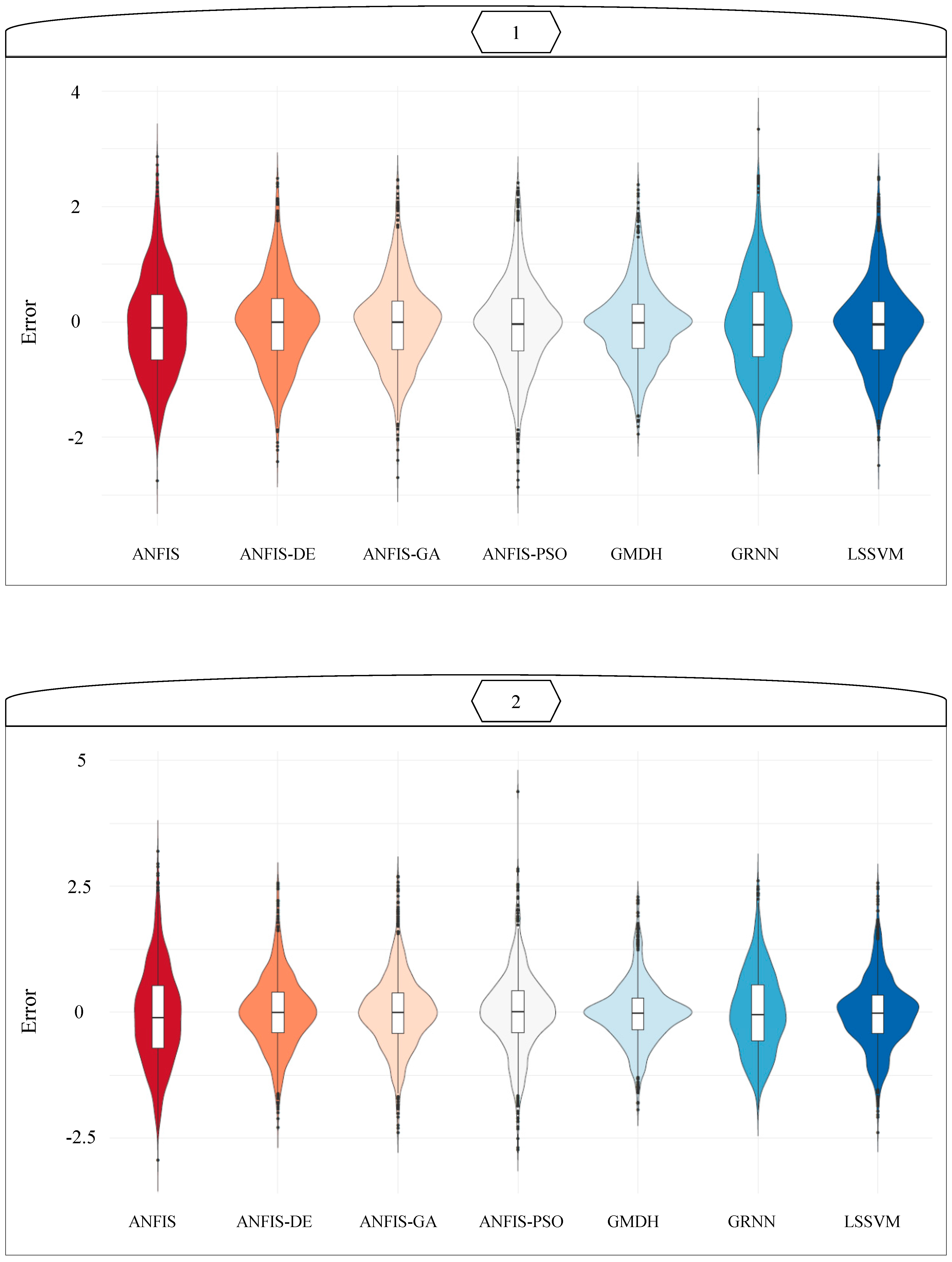
3.4. Models’ Comparisons

In this section, a Taylor diagram was used for comparing the overall performance of the models in such a way that the entire outputs of each model for the entire stations were evaluated against the real values of the indices (Figure 6).

The diagram exhibits the error rate, correlation coefficient and the standard deviation of the estimated values in comparison to the observed amounts [57,58]. Taylor diagrams (Figure 6) show that ANFIS and GRNN have had the lowest accuracy in contrast to the other models in terms of both of the suggested inputs (entropy theory and gamma test), and GMDH was found with the best predictions. It can be stated, according to the Taylor diagram, that the models’ predictions are more correlated and less erroneous when applying the inputs of entropy theory. Furthermore, the standard deviation of the outputs also approaches the real values to some extent, with the use of entropy theory’s inputs. In diagrams related to JDI, the maximum value of R is about 0.7, and the minimum value of RMSE is about 0.65 that is pertinent to the GMDH model and entropy theory. MSPI diagrams also confirm that GMDH (especially with entropy theory’s inputs) has the best performance with RMSE below 0.5 and R found to be about 0.9. In this case (MSPI with entropy theory’s inputs), the standard deviation values of the predicted data are closest to that of the observed data.

The models’ error distributions are shown in violin plots (Figure 7). In this violin plot, the entire errors of each model (for all the stations) were delineated for each index. It can be seminally observed that the violin’s curvature is softer in the violin plots drawn for ANFIS and GRNN models. This is reflective of the idea that these two models’ errors have relatively more uniform distribution than the other models; or, in other words, the errors’ frequencies slightly differ between the larger and smaller values, and the errors with larger values are relatively more frequent in these two models. In the ANFIS-PSO model and, after this, in LSSVM, ANFIS-GA and ANFIS-DE models, the violins’ curvatures are reduced and their frequency is gradually increased about zero error. In the GMDH model, this issue reaches its peak point in such a way that the GMDH model’s errors feature the highest frequency about zero in all the four diagrams of Figure 7. The issue can be clearly seen in the MSPI’s outputs.

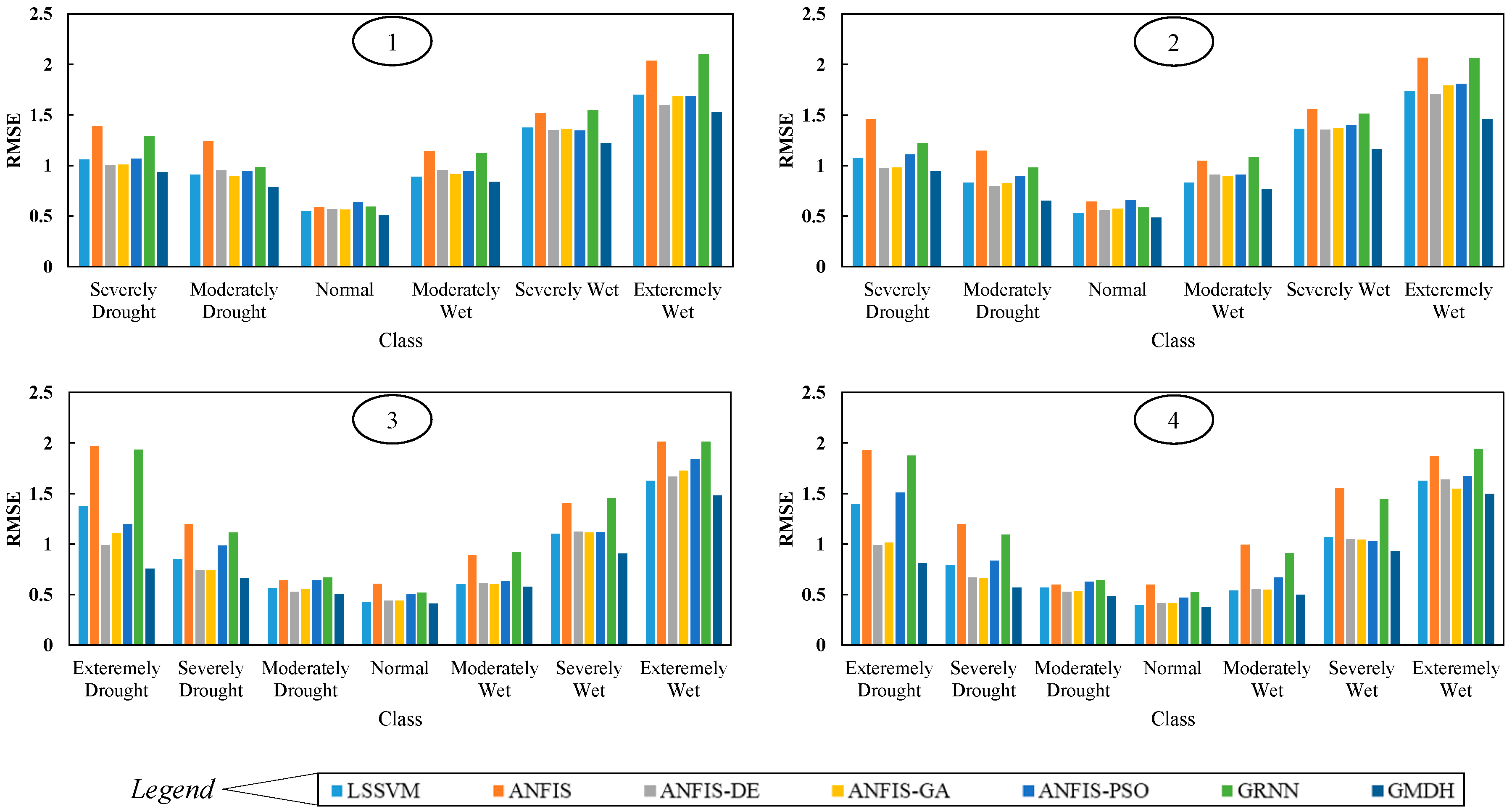
3.5. Evaluation of the Models’ Accuracy in Drought Classes

In this part of the present study, the models’ errors are evaluated with regard to the various drought classes. Something that draws attention at first glance in Figure 8 is that JDI is one class shorter than MSPI.

The reason for this issue is JDI’s weakness in showing the very severe droughts, and it had been previously examined by Bazrafshan et al. [2]. Considering Figure 8, MSPI takes a smaller RMSE value in comparison to JDI for all of the drought classes. The lowest prediction error pertains to the normal class, and the RMSE value is increased after this with the increase in the intensity of drought or wetness. It can also be observed that drought is predicted with smaller errors in contrast to wetness for identical intensities. For instance, in MSPI predictions based on the inputs suggested by entropy theory, RMSE value was smaller in severe drought periods than severe wetness periods and/or more accurate predictions were offered by the models for the very severe drought periods as compared to very intensive wetness periods. In addition, in predicting moderate and severe droughts (for both MSPI and JDI) as well as predicting very severe droughts (MSPI), GMDH followed by ANFIS-DE and ANFIS-GA can be trusted to give more reliable results compared to other models.

4. Discussion

Forecasting JDI has not been found among the previous studies up to now. MSPI forecasting was found only in one study [11] that is getting discussed. Aghelpour et al. [11] used the GA & PSO algorithms to optimize ANFIS, and there are also similar stations (Isfahan & Yazd). Comparing these two prediction studies shows that the similar models, including ANFIS, ANFIS-GA & ANFIS-PSO, had better performances for these two stations, in the research of Aghelpour et al. [11]. There are similarities between the models and stations; so, the difference can only be related to the time windows. In Aghelpour et al. [11], the prediction was implemented for the time windows MSPI9-12, but in the current study, MSPI_1–12 was investigated. MSPI_9–12 is an index of agricultural drought and deal with about one type of drought. However, MSPI_1–12 is an index for three types of droughts, including meteorological, hydrological and agricultural drought simultaneously. In predicting three types of droughts simultaneously, more error is completely normal, compared to predicting just one type of drought.

In comparing the two multivariate drought indices, these prediction results can complement the study by Bazrafshan et al. [2]. They found MSPI is more appropriate than JDI for monitoring multivariate drought status in Iran. The present study adds that MSPI predictions are also more accurate than JDI’s. Hence, it can be stated that the MSPI is more appropriate for both monitoring and predicting multivariate droughts compared to JDI in Iran.

5. Conclusions

Machine learning models have good accuracies for predicting multivariate drought based on JDI and MSPI and can be considered good alternatives among the models that can provide short-term predictions.

Among the studied models, GMDH was found to have the best accuracy and is suggested to be employed for multivariate drought predictions. The reason for that the number of parameters in this model is more than the other models. The number of layers and neurons in GMDH is changeable and creates a large range of network make-up, whereas GRNN has only spread parameters. The optimizers of ANFIS, including DE, GA and PSO, could improve the ANFIS’s accuracy by 39.4%, 38.7% and 22.6%, respectively. Hence, in multivariate drought forecasting, the use of DE and GA is suggested.

On the other hand, according to the results of the gamma test and entropy theory, precipitation and temperature values of the previous months (in addition to the past amounts of the indices) are also influential in forecasting multivariate drought. Hence, the use of these variables as the models’ inputs is suggested for predicting the general status of the drought. None of the two methods of input selection for short-term prediction of the indices proposed in the current research can be decisively considered superior to the other, but entropy theory seems to be more promising according to the general results. Generally, forecasting some different types of drought together (e.g., meteorological, hydrological and agricultural droughts simultaneously) by the current method is a “theoretical study” and to be changed to an “applied study”, it is suggested to validate the indices by the actual simultaneous events of these different drought types.

References

1. Abbaspour, M.; Sabetraftar, A. Review of cycles and indices of drought and their effect on water resources, ecological, biological, agricultural, social and economical issues in Iran. Int. J. Environ. Stud. 2005, 62, 709–724. [Google Scholar] [CrossRef]
2. Bazrafshan, J.; Nadi, M.; Ghorbani, K. Comparison of Empirical Copula-Based Joint Deficit Index (JDI) and Multivariate Standardized Precipitation Index (MSPI) for Drought Monitoring in Iran. Water Resour. Manag. 2015, 29, 2027–2044. [Google Scholar] [CrossRef]
3. Bai, X.; Wang, Y.; Jin, J.; Ning, S.; Wang, Y.; Wu, C. Spatio-Temporal Evolution Analysis of Drought Based on Cloud Transformation Algorithm over Northern Anhui Province. Entropy 2020, 22, 106. [Google Scholar] [CrossRef] [Green Version]
4. Svoboda, M.; Hayes, M.; Wood, D. Standradized Precipitation Index User Guide; World Meteorological Organization: Geneva, Switzerland, 2012; Volume 21, pp. 1333–1348. [Google Scholar] [CrossRef] [Green Version]
5. Kao, S.C.; Govindaraju, R.S. A copula-based joint deficit index for droughts. J. Hydrol. 2010, 380, 121–134. [Google Scholar] [CrossRef]
6. Mirabbasi, R.; Anagnostou, E.N.; Fakheri-Fard, A.; Dinpashoh, Y.; Eslamian, S. Analysis of meteorological drought in northwest Iran using the Joint Deficit Index. J. Hydrol. 2013, 492, 35–48. [Google Scholar] [CrossRef]
7. Hao, Z.; Singh, V.P. Drought characterization from a multivariate perspective: A review. J. Hydrol. 2015, 527, 668–678. [Google Scholar] [CrossRef]
8. Ma, M.; Ren, L.; Singh, V.P.; Tu, X.; Jiang, S.; Liu, Y. Evaluation and application of the SPDI-JDI for droughts in Texas, USA. J. Hydrol. 2015, 521, 34–45. [Google Scholar] [CrossRef]
9. Bazrafshan, J.; Hejabi, S.; Rahimi, J. Drought Monitoring Using the Multivariate Standardized Precipitation Index (MSPI). Water Resour. Manag. 2014, 28, 1045–1060. [Google Scholar] [CrossRef]
10. Bateni, M.M.; Behmanesh, J.; De Michele, C.; Bazrafshan, J.; Rezaie, H. Composite agrometeorological drought index accounting for seasonality and autocorrelation. J. Hydrol. Eng. 2018, 23. [Google Scholar] [CrossRef] [Green Version]
11. Aghelpour, P.; Bahrami-Pichaghchi, H.; Kisi, O. Comparison of three different bio-inspired algorithms to improve ability of neuro fuzzy approach in prediction of agricultural drought, based on three different indexes. Comput. Electron. Agric. 2020, 170, 105279. [Google Scholar] [CrossRef]
12. Moreira, E.E.; Pires, C.L.; Pereira, L.S. SPI drought class predictions driven by the North Atlantic Oscillation index using log-linear modeling. Water 2016, 8, 43. [Google Scholar] [CrossRef] [Green Version]
13. Belayneh, A.; Adamowski, J.; Khalil, B.; Ozga-Zielinski, B. Long-term SPI drought forecasting in the Awash River Basin in Ethiopia using wavelet neural networks and wavelet support vector regression models. J. Hydrol. 2014, 508, 418–429. [Google Scholar] [CrossRef]
14. Deo, R.C.; Kisi, O.; Singh, V.P. Drought forecasting in eastern Australia using multivariate adaptive regression spline, least square support vector machine and M5Tree model. Atmos. Res. 2017, 184, 149–175. [Google Scholar] [CrossRef] [Green Version]
15. Mokhtarzad, M.; Eskandari, F.; Jamshidi Vanjani, N.; Arabasadi, A. Drought forecasting by ANN, ANFIS, and SVM and comparison of the models. Environ. Earth Sci. 2017, 76, 729. [Google Scholar] [CrossRef]
16. Zahraie, B.; Nasseri, M.; Nematizadeh, F. Exploring spatiotemporal meteorological correlations for basin scale meteorological drought forecasting using data mining methods. Arab. J. Geosci. 2017, 10, 419. [Google Scholar] [CrossRef]
17. Chen, M.; Ning, S.; Cui, Y.; Jin, J.; Zhou, Y.; Wu, C. Quantitative assessment and diagnosis for regional agricultural drought resilience based on set pair analysis and connection entropy. Entropy 2019, 21, 373. [Google Scholar] [CrossRef] [Green Version]
18. Deo, R.C.; Şahin, M. Application of the Artificial Neural Network model for prediction of monthly Standardized Precipitation and Evapotranspiration Index using hydrometeorological parameters and climate indices in eastern Australia. Atmos. Res. 2015, 161, 65–81. [Google Scholar] [CrossRef]
19. Maca, P.; Pech, P. Forecasting SPEI and SPI drought indices using the integrated artificial neural networks. Comput. Intell. Neurosci. 2016, 2016, 3868519. [Google Scholar] [CrossRef] [Green Version]
20. Soh, Y.W.; Koo, C.H.; Huang, Y.F.; Fung, K.F. Application of artificial intelligence models for the prediction of standardized precipitation evapotranspiration index (SPEI) at Langat River Basin, Malaysia. Comput. Electron. Agric. 2018, 144, 164–173. [Google Scholar] [CrossRef]
21. Tian, Y.; Xu, Y.P.; Wang, G. Agricultural drought prediction using climate indices based on Support Vector Regression in Xiangjiang River basin. Sci. Total Environ. 2018, 622, 710–720. [Google Scholar] [CrossRef]
22. Mohammadi, B.; Guan, Y.; Aghelpour, P.; Emamgholizadeh, S.; Pillco Zolá, R.; Zhang, D. Simulation of Titicaca Lake Water Level Fluctuations Using Hybrid Machine Learning Technique Integrated with Grey Wolf Optimizer Algorithm. Water 2020, 12, 3015. [Google Scholar] [CrossRef]
23. Kisi, O.; Gorgij, A.D.; Zounemat-Kermani, M.; Mahdavi-Meymand, A.; Kim, S. Drought forecasting using novel heuristic methods in a semi-arid environment. J. Hydrol. 2019, 578, 124053. [Google Scholar] [CrossRef]
24. Malik, A.; Kumar, A.; Singh, R.P. Application of heuristic approaches for prediction of hydrological drought using multi-scalar streamflow drought index. Water Resour. Manag. 2019, 33, 3985–4006. [Google Scholar] [CrossRef]
25. Ahmadi, A.; Han, D.; Karamouz, M.; Remesan, R. Input data selection for solar radiation estimation. Hydrol. Process. 2009, 23, 2754–2764. [Google Scholar] [CrossRef]
26. Remesan, R.; Shamim, M.A.; Han, D. Model data selection using gamma test for daily solar radiation estimation. Hydrol. Process. 2008, 22, 4301–4309. [Google Scholar] [CrossRef]
27. Ashrafzadeh, A.; Ghorbani, M.A.; Biazar, S.M.; Yaseen, Z.M. Evaporation process modelling over northern Iran: Application of an integrative data-intelligence model with the krill herd optimization algorithm. Hydrol. Sci. J. 2019, 64, 1843–1856. [Google Scholar] [CrossRef]
28. Khaledian, M.R.; Isazadeh, M.; Biazar, S.M.; Pham, Q.B. Simulating Caspian Sea surface water level by artificial neural network and support vector machine models. Acta Geophys. 2020, 68, 553–563. [Google Scholar] [CrossRef]
29. Rahimi, J.; Ebrahimpour, M.; Khalili, A. Spatial changes of Extended De Martonne climatic zones affected by climate change in Iran. Theor. Appl. Climatol. 2013, 112, 409–418. [Google Scholar] [CrossRef]
30. McKee, T.B.; Doesken, N.J.; Kleist, J. The relationship of drought frequency and duration to time scales. In Proceedings of the 8th Conference on Applied Climatology, Boston, MA, USA, 17–22 January 1993; Volume 17, pp. 179–183. [Google Scholar]
31. Evans, D.; Jones, A.J. A proof of the Gamma test. Proc. R. Soc. A Math. Phys. Eng. Sci. 2002, 458, 2759–2799. [Google Scholar] [CrossRef]
32. Moghaddamnia, A.; Ghafari Gousheh, M.; Piri, J.; Amin, S.; Han, D. Evaporation estimation using artificial neural networks and adaptive neuro-fuzzy inference system techniques. Adv. Water Resour. 2009, 32, 88–97. [Google Scholar] [CrossRef]
33. Shannon, C.E. A Mathematical Theory of Communication. Bell Syst. Tech. J. 1948, 27, 379–423. [Google Scholar] [CrossRef] [Green Version]
34. Cheng, L.; Niu, J.; Liao, D. Entropy-based investigation on the precipitation variability over the Hexi Corridor in China. Entropy 2017, 19, 660. [Google Scholar] [CrossRef] [Green Version]
35. Reza, F.M. An Introduction to Information Theory; Courier Corporation: North Chelmsford, MA, USA, 1994; ISBN 0486682102. [Google Scholar]
36. Mohammadi, B.; Linh, N.T.T.; Pham, Q.B.; Ahmed, A.N.; Vojteková, J.; Guan, Y.; Abba, S.I.; El-Shafie, A. Adaptive neuro-fuzzy inference system coupled with shuffled frog leaping algorithm for predicting river streamflow time series. Hydrol. Sci. J. 2020, 65. [Google Scholar] [CrossRef]
37. Jang, J.S.R. ANFIS: Adaptive-Network-Based Fuzzy Inference System. IEEE Trans. Syst. Man Cybern. 1993, 23, 665–685. [Google Scholar] [CrossRef]
38. Storn, R.; Price, K. Differential Evolution—A Simple and Efficient Heuristic for Global Optimization over Continuous Spaces. J. Glob. Optim. 1997, 11, 341–359. [Google Scholar] [CrossRef]
39. Halabi, L.M.; Mekhilef, S.; Hossain, M. Performance evaluation of hybrid adaptive neuro-fuzzy inference system models for predicting monthly global solar radiation. Appl. Energy 2018, 213, 247–261. [Google Scholar] [CrossRef]
40. Holland, J.H. Adaptation in Natural and Artificial Systems; MT Press: Berkeley, CA, USA, 2019. [Google Scholar]
41. Jahani, B.; Mohammadi, B. A comparison between the application of empirical and ANN methods for estimation of daily global solar radiation in Iran. Theor. Appl. Climatol. 2019, 137, 1257–1269. [Google Scholar] [CrossRef]
42. Jaramillo, J.H.; Bhadury, J.; Batta, R. On the use of genetic algorithms to solve location problems. Comput. Oper. Res. 2002, 29, 761–779. [Google Scholar] [CrossRef]
43. Eberhart, R.; Kennedy, J. New optimizer using particle swarm theory. In Proceedings of the International Symposium on Micro Machine and Human Science, Nagoya, Japan, 4–6 October 1995. [Google Scholar]
44. Mohammadi, B.; Ahmadi, F.; Mehdizadeh, S.; Guan, Y.; Pham, Q.B.; Linh, N.T.T.; Tri, D.Q. Developing Novel Robust Models to Improve the Accuracy of Daily Streamflow Modeling. Water Resour. Manag. 2020, 34, 3387–3409. [Google Scholar] [CrossRef]
45. Ivakhnenko, A.G. Heuristic self-organization in problems of engineering cybernetics. Automatica 1970, 6, 207–219. [Google Scholar] [CrossRef]
46. Aghelpour, P.; Varshavian, V. Evaluation of stochastic and artificial intelligence models in modeling and predicting of river daily flow time series. Stoch. Environ. Res. Risk Assess. 2020, 34, 33–50. [Google Scholar] [CrossRef]
47. Ashrafzadeh, A.; Kişi, O.; Aghelpour, P.; Biazar, S.M.; Masouleh, M.A. Comparative study of time series models, support vector machines, and GMDH in forecasting long-term evapotranspiration rates in northern Iran. J. Irrig. Drain. Eng. 2020, 146, 4020010. [Google Scholar] [CrossRef]
48. Aghelpour, P.; Guan, Y.; Bahrami-Pichaghchi, H.; Mohammadi, B.; Kisi, O.; Zhang, D. Using the MODIS Sensor for Snow Cover Modeling and the Assessment of Drought Effects on Snow Cover in a Mountainous Area. Remote Sens. 2020, 12, 3437. [Google Scholar] [CrossRef]
49. Araghinejad, S. Data-Driven Modeling: Using MATLAB® in Water Resources and Environmental Engineering; Springer Science and Business Media: Berlin, Germany, 2014; Volume 67. [Google Scholar]
50. Houichi, L.; Dechemi, N.; Heddam, S.; Achour, B. An evaluation of ANN methods for estimating the lengths of hydraulic jumps in U-shaped channel. J. Hydroinform. 2013, 15, 147–154. [Google Scholar] [CrossRef]
51. Suykens, J.A.K.; Vandewalle, J. Least squares support vector machine classifiers. Neural Process. Lett. 1999, 9, 293–300. [Google Scholar] [CrossRef]
52. Mohammadi, B.; Mehdizadeh, S. Modeling daily reference evapotranspiration via a novel approach based on support vector regression coupled with whale optimization algorithm. Agric. Water Manag. 2020, 237, 106145. [Google Scholar] [CrossRef]
53. Moazenzadeh, R.; Mohammadi, B. Assessment of bio-inspired metaheuristic optimisation algorithms for estimating soil temperature. Geoderma 2019, 353, 152–171. [Google Scholar] [CrossRef]
54. Mohammadi, B.; Aghashariatmadari, Z. Estimation of solar radiation using neighboring stations through hybrid support vector regression boosted by Krill Herd algorithm. Arab. J. Geosci. 2020, 13, 1–16. [Google Scholar] [CrossRef]
55. Guan, Y.; Mohammadi, B.; Pham, Q.B.; Adarsh, S.; Balkhair, K.S.; Rahman, K.U.; Linh, N.T.T.; Tri, D.Q. A novel approach for predicting daily pan evaporation in the coastal regions of Iran using support vector regression coupled with krill herd algorithm model. Theor. Appl. Climatol. 2020, 142, 349–367. [Google Scholar] [CrossRef]
56. Biazar, S.M.; Fard, A.F.; Singh, V.P.; Dinpashoh, Y.; Majnooni-Heris, A. Estimation of Evaporation from Saline-Water with More Efficient Input Variables. Pure Appl. Geophys. 2020, 177, 5599–5619. [Google Scholar] [CrossRef]
57. Biazar, S.M.; Fard, A.F.; Singh, V.P.; Dinpashoh, Y.; Majnooni-Heris, A. Estimation of evaporation from saline water. Environ. Monit. Assess. 2020, 192, 1–17. [Google Scholar] [CrossRef] [PubMed]
58. Aghelpour, P.; Mohammadi, B.; Biazar, S.M. Long-term monthly average temperature forecasting in some climate types of Iran, using the models SARIMA, SVR, and SVR-FA. Theor. Appl. Climatol. 2019, 138, 1471–1480. [Google Scholar] [CrossRef]
Figure 1. Situation of the intended stations in Iran.
Ijgi 09 00701 g001
Figure 2. Schematic form of adaptive neuro-fuzzy inference system (ANFIS) merging with the algorithms differential evolution (DE), genetic algorithm (GA) and particle swarm optimization (PSO).
Ijgi 09 00701 g002
Figure 3. The variation of forecasts and observations for the JDI prediction in all of the stations; The numbers of the subplots refer to the stations including Anar (1), Biarjmand (2), Boshrouyeh (3), East Isfahan (4), Isfahan (5), Kabootarabad (6), Kashan (7), Marvast (8), Naein (9) and Yazd (10).
Ijgi 09 00701 g003
Figure 4. The variation of forecasts and observations for the MSPI prediction in all of the stations; The numbers of the subplots refer to the stations including Anar (1), Biarjmand (2), Boshrouyeh (3), East Isfahan (4), Isfahan (5), Kabootarabad (6), Kashan (7), Marvast (8), Naein (9) and Yazd (10).
Ijgi 09 00701 g004
Figure 5. Scatter plots in comparing the performances of the gamma test and entropy theory for MSPI and JDI prediction (Marvast station).
Ijgi 09 00701 g005
Figure 6. Taylor diagrams of the model prediction; Total evaluation of JDI’s predictions by inputs of gamma test (1) and entropy theory (2) and total evaluation of MSPI’s predictions by inputs of gamma test (3) and entropy theory (4).
Ijgi 09 00701 g006
Figure 7. Violin plots of the errors; Total evaluation of JDI’s prediction error resulted by inputs of gamma test (1) and entropy theory (2) and total evaluation of MSPI’s prediction error resulted by inputs of gamma test (3) and entropy theory (4).
Ijgi 09 00701 g007aIjgi 09 00701 g007b
Figure 8. Root mean squared error (RMSE) values in drought classes; JDI’s prediction resulted by inputs of gamma test (1) and entropy theory (2) and MSPI’s prediction resulted by inputs of gamma test (3) and entropy theory (4).
Ijgi 09 00701 g008