Geodiversity Assessment with Crowdsourced Data and Spatial Multicriteria Analysis

Abstract

This paper presents an approach to geodiversity assessment based on spatial multicriteria analysis. Instead of relying solely on weighted linear combination (WLC) for aggregating factor ratings and weights to compute a synthetic measure of geodiversity, the approach employs WLC in concert with its local version called L-WLC to provide a more comprehensive assessment approach. As part of the approach, the assessment input data comprised of geodiversity factor ratings and weights were obtained through crowdsourcing. A geoinformation crowdsourcing tool called the geo-questionnaire was used to obtain data from 57 Earth science researchers worldwide. These data served as the bases for a group assessment of geodiversity. The reliability of assessment was evaluated by means of spatially explicit uncertainty analysis. The results showed the efficacy of local spatial multicriteria analysis techniques (L-WLC) used in concert with a global technique (WLC) on the example of geodiversity assessment for Karkonosze National Park in southwestern Poland.

1. Introduction

Geodiversity denotes variability in abiotic components in a hierarchical ecological system that includes geology, Earth surface relief, soil cover, surface and ground water, and climate [1,2,3,4]. Arguably, geodiversity determines biotic conditions and by extension biodiversity. However, despite the relationship, the concept of geodiversity is much less known than biodiversity. Although geodiversity underpins biodiversity, it does have a stand-alone scientific and practical value. Information on geodiversity can aid the assessment of protected areas (e.g., national parks, reserves, geoparks, and geosites) or comparative studies of special interest areas. Undoubtedly, the value of geodiversity is instrumental for geotourism, geoheritage and geoconservation, which indicates a significant interdisciplinary nature of geodiversity [5]. The benefits of geodiversity assessment include, among others, better understanding of geo-ecosystem functioning, facilitating the management of protected areas, and more complete valuation of ecosystem services [6]. These benefits are of paramount importance in the age of global warming and accelerated land use/land cover change.

While the value of geodiversity is established, the methods of assessing it are not. Geodiversity assessment methods include, among others, descriptive methods, geodiversity indexes, and GIS-based suitability analysis [7]. Each of these methods introduces an ambiguity by way of relying on expert judgement rather than on direct measurement. The ambiguity, in turn, compromises the robustness of geodiversity assessment.

Geodiversity assessment typically involves an individual expert or a group of experts who judge the contribution value of geodiversity factors to the overall geodiversity score for a given geographical area. The contribution of each factor is expressed by a rating value selected from a standardized scale, e.g., a Likert 1–5 scale [7]. In the case of GIS-based suitability analysis, experts judge in addition to ratings the importance of each factor relative to other geodiversity factors and express it with a numeric weight, e.g., an integer value ranging between 0 and 100 in the case of percentages [8]. Rating scores and weights need to be aggregated to calculate the overall geodiversity score. Judgement aggregation in geodiversity assessment is analogous to judgment aggregation in group decision making and can follow one of two scenarios [9]. Under the first scenario, individual ratings and weights are aggregated into a collective set of rating scores and weights used next to calculate the overall geodiversity score for each area. Under the second scenario, the individual expert ratings and weights are initially used to compute the geodiversity scores for each analysis unit. Then, the geodiversity scores are aggregated for each unit using an aggregation rule (e.g., an arithmetic, geometric, or harmonic mean). While the former approach has been used in previous geodiversity assessment studies (e.g., [7,8]), the latter approach has not.

A common aggregation rule for calculating geodiversity assessment scores is weighted linear combination (WLC) [7,10,11]. The result of WLC aggregation for each spatial unit under assessment is a geodiversity score represented by the sum of factor ratings and weights. WLC has been widely used in calculating composite indicators for policy monitoring, public communication, and environmental assessment [12] and in spatial multicriteria analysis [9,13]. The appeal of WLC as a multiple attribute aggregation rule is obvious: weighted sum is an aggregate value that is easy to calculate and comprehend. In an assessment problem where WLC is applied to calculate a geodiversity score for each spatial unit, a factor weight is assumed to be constant over the study area irrespective of the intrinsic factor’s variability. This approach does not account for differences in spatial variability among the geodiversity factors. A local approach to WLC (L-WLC) proposed by Malczewski [14] accounts for a factor’s spatial variability by way of factor weights calculated in each neighborhood comprised of multiple spatial units. This approach opens up the possibility of analyzing geodiversity by explicitly accounting for local (neighborhood-based) differences and comparing it with the geodiversity assessed with a less granular(global) approach (WLC). By analogy to image processing, the local approach (L-WLC) can be compared to high-pass filter that captures local variation (high-frequency patterns) in the immediate surroundings of each spatial unit comprising a study area, whereas the global approach (WLC) resembles a low-pass filter that registers regional variations (low-frequency patterns). Combined, the two approaches to geodiversity assessment—local and global, have the potential to facilitate a more complete assessment than either one of them when used individually, yet they have not been used in concert before.

In geodiversity assessment, factor ratings and weights are typically assessed by experts who are recruited from Earth science specialists, geo-ecologists, and natural resources managers. In this paper, we introduce a crowdsourcing approach that uses an online questionnaire linked with an interactive map called geo-questionnaire [15,16]. The approach has been used in the study to collect data on geodiversity factor ratings and weights from Earth scientists worldwide with diverse interest in geodiversity. The collected data were used to implement the geodiversity assessment for Karkonosze National Park in southwestern Poland using the local and global approaches based on WLC and L-WLC aggregation rules.

In the remainder of the paper, we present the study methods, including a brief description of the study area, a geo-questionnaire for crowdsourcing data on factor ratings and weights, and WLC and L-WLC aggregation rules used for calculating the geodiversity assessment scores. We also describe the data processing steps leading to the implementation of WLC and L-WLC. Following the method description, we compare and discuss the results obtained with local (L-WLC) and global (WLC) aggregation techniques. We conclude the paper with a brief summary and future research recommendations.

2. Methods

2.1. Data Crowdsourcing and Geo-Questionnaire

Geoinformation crowdsourcing is increasingly becoming an important source of geographic information [17]. In general, geoinformation crowdsourcing involves citizens passively or actively contributing data to a data collection effort organized by scientists (i.e., citizen science), volunteers (e.g., Open Street Map), local agencies (i.e., public participation GIS) and for-profit entities (e.g., Wikimapia). In this study, we have used a geoinformation crowdsourcing approach to engage Earth science experts instead of lay citizens. The logic behind this approach takes after the idea of “wisdom of the crowd” [18], which dates back to Aristotle [19] and is well established in philosophy of science and in practice. The basic tenant of this idea is that a collective judgement of a group of individuals (e.g., experts) represented by an average of individual judgements cancels out an idiosyncratic noise introduced by an individual judgement, yielding in effect a superior estimate of phenomenon in comparison to the estimate of the individual expert. The important caveat here is that the quality of estimate is expected to improve with the number of collected judgements. However, unlike the phenomena, for which the true value can be empirically established and used as the basis for evaluating the quality of estimate, there is no such true value for geodiversity. Geodiversity is a synthetic category that can only be assessed rather than measured directly. That said, following the logic of wisdom of the crowds, one can reasonably expect the geodiversity scores resulting from crowdsourcing effort to be superior to those from an individual who specializes in a sub-field of Earth science.

To facilitate crowdsourcing, we used a geo-questionnaire. A geo-questionnaire is a web application that includes a multi-page online questionnaire with potentially various types of questions (single check box, choice list, poll, multiple choice grid, numeric slider, range, and open text field) combined with a capability to mark geographical features (e.g., points, polylines, and polygons) on an interactive map [16,20]. Map interactivity is achieved by programming in a geo-questionnaire follow-up questions that ask a respondent to substantiate/provide additional information about marked locations. Features may also be marked/delineated by selecting objects comprising a map—typically in a GeoJSON format map layer. GeoJSON is an open spatial data format supporting the encoding of various geometry types. Multiple applications of geo-questionnaires, albeit under different configurations and using different software tools, have been reported by Kahila and Kyttä [21], Brown and Weber [22], Chaix et al. [23], Jankowski et al. [24], and Haklay et al. [25]. Within the geodiversity context, this has been the first application of s geo-questionnaire to collect data for geodiversity assessment.

2.2. Local Weighted Linear Combination (L-WLC)

The L-WLC aggregation technique [14] takes into account the spatial heterogeneity of data by employing the range sensitivity principle [26]. According to the principle, factors with larger value ranges should be given greater weights than factors with smaller value ranges, that is, factors with larger value ranges are perceived as more important than factor with smaller ranges. Thus, for a factor of relief energy that shows the majority of study area within a narrow range of relief energy values, local weights will be low—in accordance with the principle. Conversely, for another factor, such as the topographic wetness index (TWI), which exhibits more spatial variability in the TWI values, local weights will be higher.

A local weight is the function of factor values in a local neighborhood (local value range), factor values in the entire study area (global value range), and a global weight assigned to the factor in question [14]:

$$w_k^q=\frac{\frac{w_k{r}_k^q}{r_k}}{{{\displaystyle \sum }}_{k=1}^n\frac{w_k{r}_k^q}{r_k}} 0\le w_k^q\le 1 and {\displaystyle \sum }_{k=1}^n{w}_k^q=1$$

(1)

where $w_k^q$ denotes the local weight of factor (k) in the neighborhood (q);

$r_k^q$ denotes the value range of factor (k) in the neighborhood (q);

$r_k$ denotes the global value range factor (k);

$w_k$ denotes the global weight factor (k).

The distinction between local and global weights should be intuitively obvious. The former vary locally depending on the local diversity of factor values, while the latter are constant for the entire study area—like in traditional non-spatial WLC (or the analytic hierarchy process (AHP)). The locally dependent weights make L-WLC a distinctly spatial method of multicriteria analysis. The crucial issue in L-WLC is the selection of proper neighborhood for calculating local value ranges and consequently local weights. The neighborhood selection is an experimental process, and the main selection guideline is to choose the shape and size of neighborhood to ensure that sufficient local variability is captured such that the number of local weights that equal zero (observe that if the range of local values equals zero, the corresponding local weight also equals zero) be minimized. In practice, this means that for homogenous data distribution with a little factor value variability, the neighborhood size should be much larger than that of heterogeneous data distribution.

3. Data and Analysis

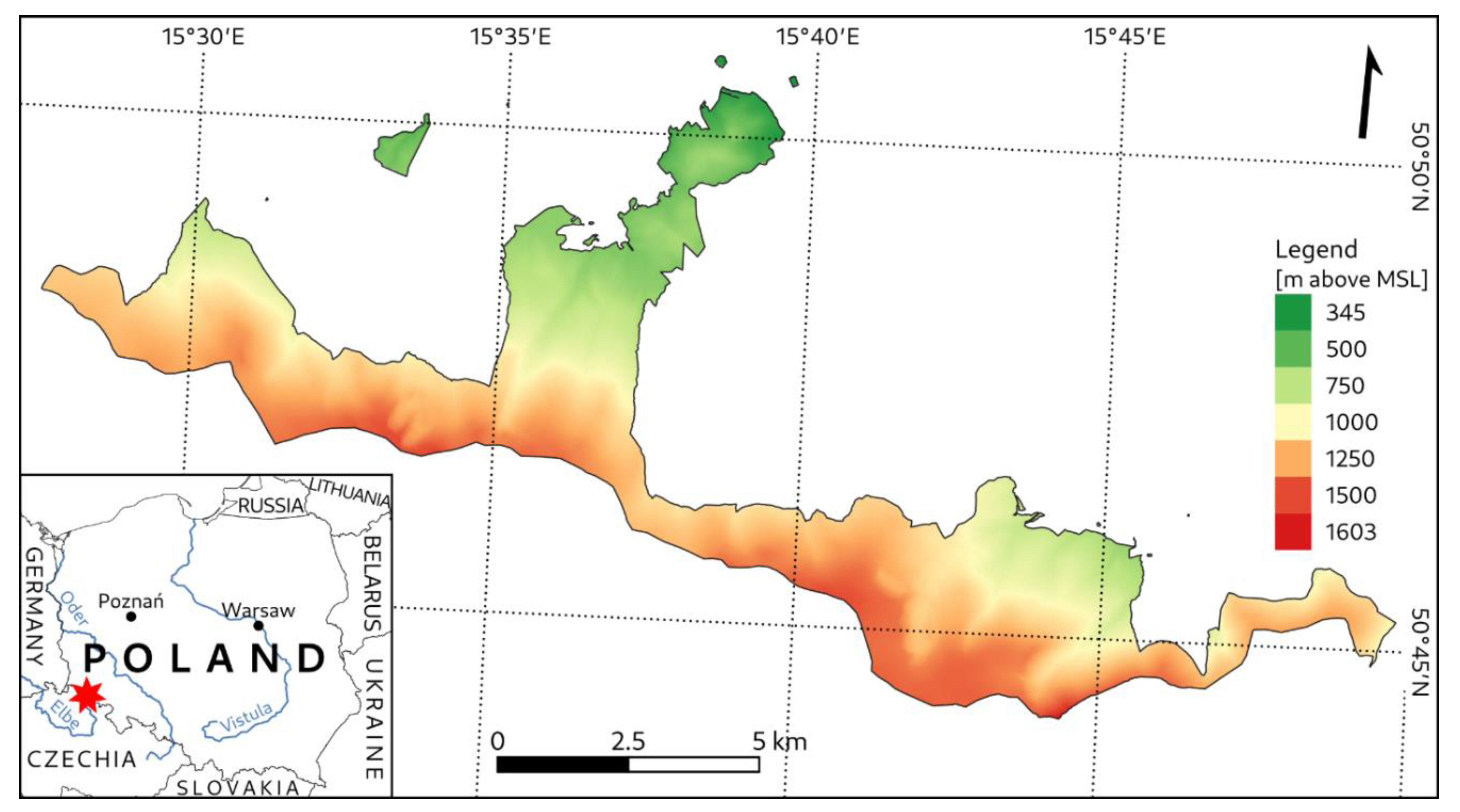
3.1. Study Area

Karkonosze National Park (KNP) is located in southwestern Poland in the border area between Poland and the Czech Republic, and it occupies the area of 59.5 km² (Figure 1). Karkonosze is the highest mountain range of the Sudetes [27]. The park also includes one enclave in the Karkonosze Foothills: waterfall Szklarka. The uniqueness of Karkonosze and its landscape is underscored by the presence of altitudinally highest and the second highest climate–vegetation zones: alpine and subalpine, despite the top altitude rising only to the modest 1603 m a.s.l. (Mt. Śnieżka). Within the park enclave, there are well-preserved submontane and lower montane forests (primarily beech forests). The most valuable asset of Karkonosze is their Pleistocene postglacial relief represented by glacial kettles (Snow kettles with 120 m vertical walls) as well as terminal and lateral moraines. The characteristic elements of the Karkonosze landscape are planation surfaces and granite rocks with fanciful shapes. A peculiarity of the park is the subarctic Upa bog.

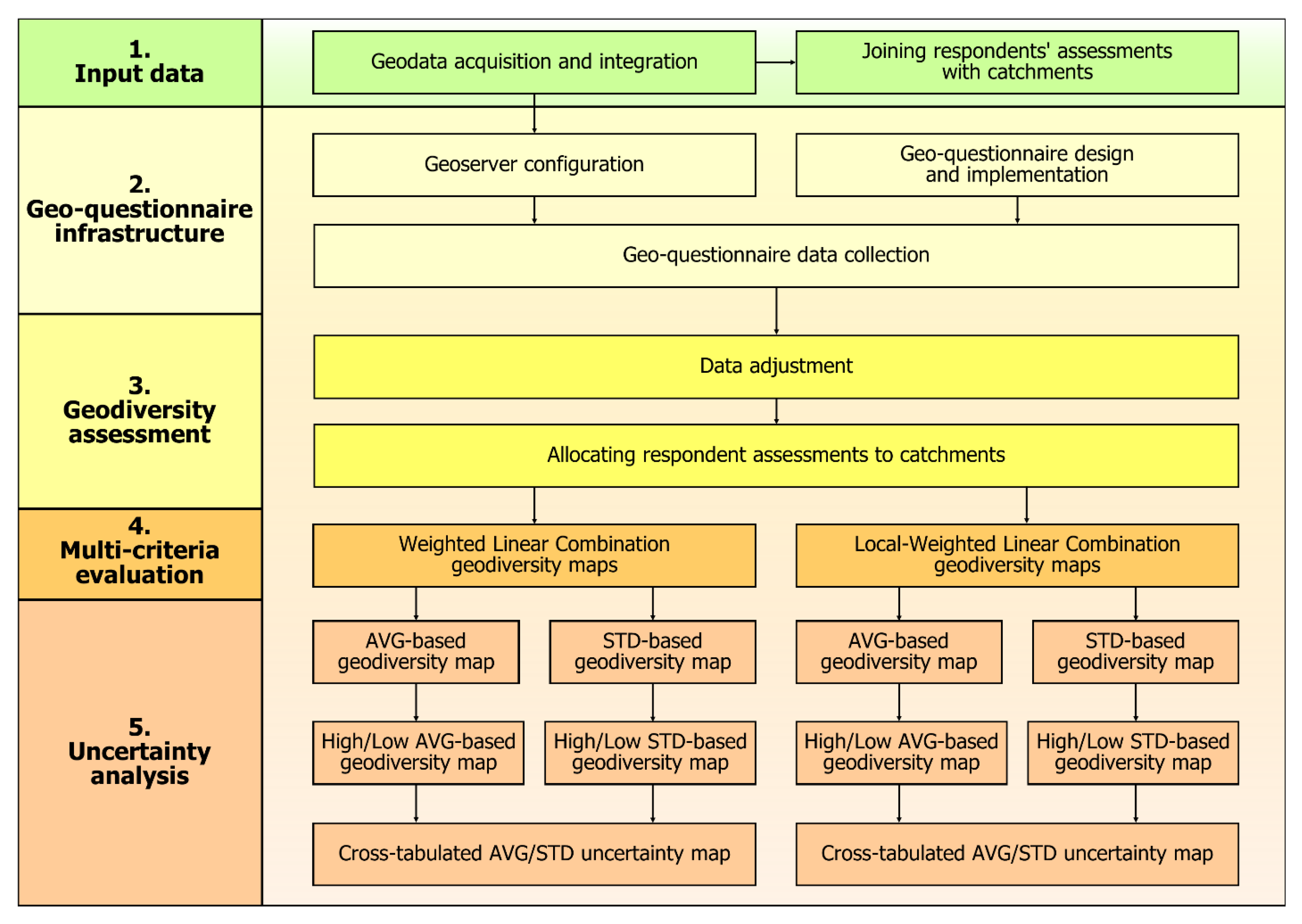
3.2. Data Processing Workflow

The geodiversity assessment for KNP involving global and local weighted linear combination rules (WLC and L-WLC) followed a workflow comprised of five tasks with subsequent steps in each task (Figure 2). The workflow tasks include: input data preparation (1. in Figure 2), geo-questionnaire infrastructure preparation (2. in Figure 2), geodiversity assessment (3. in Figure 2), multi-criteria evaluation (4. in Figure 2) and uncertainty analysis (5. in Figure 2).

The input datasets included 1 m Digital Elevation Model (DEM) [28], CORINE Land Cover [29], and thematic feature map layers, as well as lithological, geomorphological, and hydrographical soils, obtained from the GIS section of the KNP [28]—see Figure 3. The layers were integrated and transformed into the ETRS89/Poland CS92 (EPSG 2180) coordinate system. The first-order catchments were selected as map units for the geodiversity assessment. In total, 419 polygon catchments were delineated within the KNP area using the Catchment Grid Delineation tool implemented in ArcHydro 10.2—an open-source tool [30]. The burnt-out stream network, on the basis of which catchments were delineated, was verified using vector features of streams obtained from the KNP.

Bearing in mind the contemporary understanding of geodiversity, care was taken to include all factors influencing geodiversity in the research. Following the geodiversity assessment method [7,8,10,11,31], this article uses the seven following components of the geographical environment in raster-format maps: lithological features, relief energy as relative height, landforms, land cover and land use as a surrogate of landform preservation, soils, solar radiation as a surrogate of mesoclimatic conditions and the topographical wetness index as a surrogate of hydrographic conditions. They were compiled using standard GIS data processing functions for the geodiversity assessment task. The above-mentioned factors meet the conditions of commonly used definitions of geodiversity [2,3,4,32].

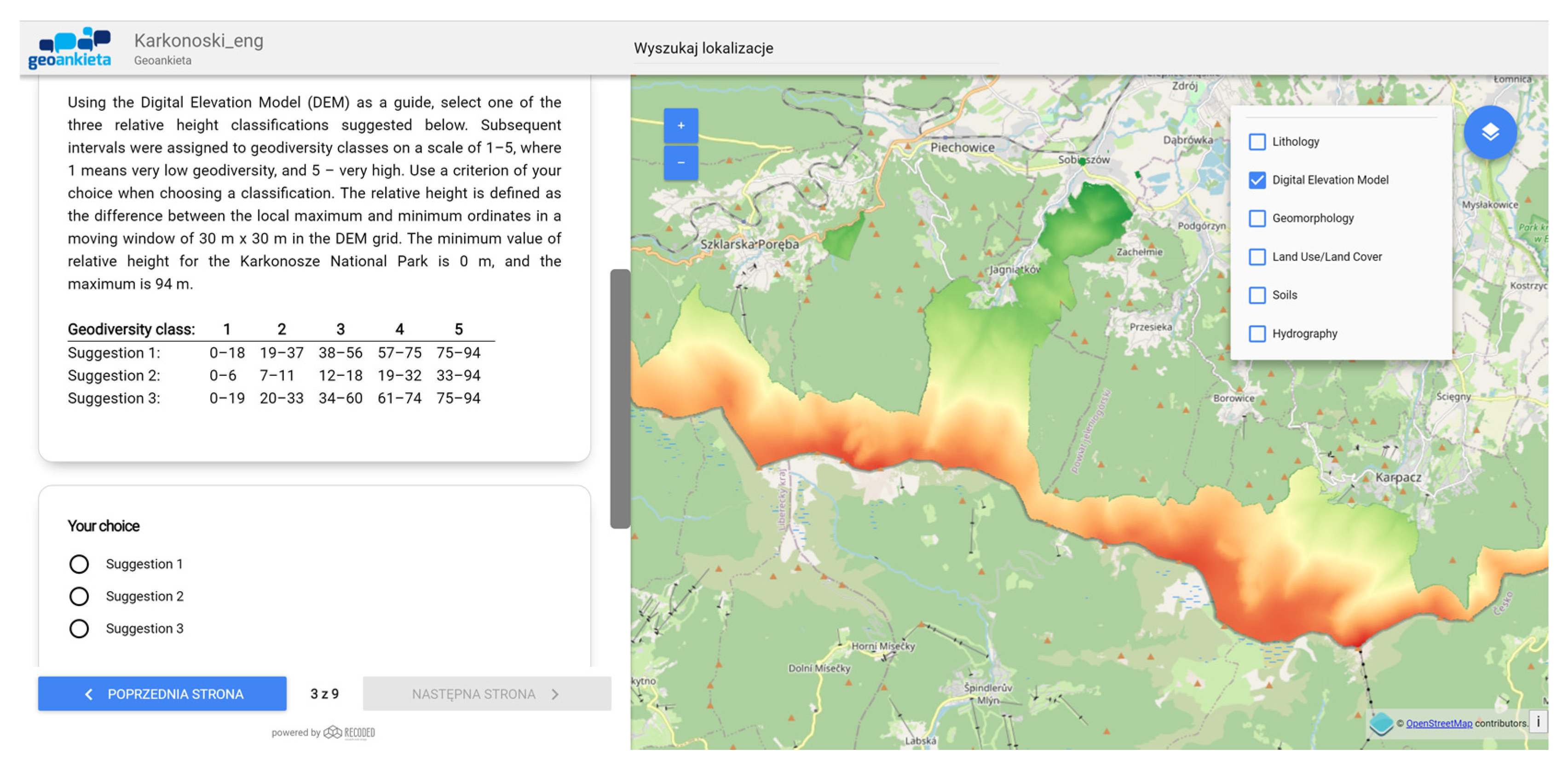
3.3. Geo-Questionnaire

The geo-questionnaire was built using an external web-based tool for custom geo-surveys, which is based on open source technology [16,20]. Using the geo-questionnaire wizard, an application can be configured in a few steps, out of which the most important are formulating questions and setting up map layers. The capability of the geo-questionnaire allowing one to link questions with map displays was leveraged to support the respondents in factor rating and weighting. The maps were served from a dedicated geoserver via Tile Map Service using the open-source GeoServer software [33]. In the map definition part of the LOPI software creation wizard, we simply provided proper web links to the tiled maps of KNP stored on the geoserver. Geo-questionnaire questions are facilitated by drag-and-drop components representing different question types, for example, slider range question, matrix answer question, number range question, or open question. The geo-questionnaire wizard is available from a vendor as an app, however, the tool can be also compiled from an open-source code available at Recoded GitLab repository [34].

The geo-questionnaire includes nine pages with page 1 for respondent contact data, pages 2–8 for responses to geodiversity factors ratings (geodiversity classes) and page 9 for responses to questions about factor weights. The geodiversity classes are assessed on a five-point Likert scale [35] with 1 representing very low geodiversity and 5 very high geodiversity (Figure 4). The geodiversity factors include lithology, relief energy (represented by relative height), geomorphology, land use/land cover (as an indicator of changes in the Earth’s surface caused by human impact), soils, mesoclimate (represented by total insolation), and hydrography (represented by the topographic wetness index). Each factor weight can be selected by using the 1–100 percentage scale, where a weight represents the relative influence of a given factor on the overall geodiversity score. Each page of the geo-questionnaire also includes an open question asking a respondent to provide a brief justification for a geodiversity factor class assignment.

Earth science researchers were contacted by the authors first in May and next in June 2020 and asked to respond to the geo-questionnaire. The estimated time required to complete the geo-questionnaire (the authors’ estimate) ranged from 40 to 50 min, but the respondents were not asked to report their time effort. The initial call (made in May 2020) resulted in 23 geo-questionnaire responses, including 11 complete and 12 incomplete. The subsequent call in June acquired 59 responses, including 46 complete and 13 incomplete. In total, out of 82 responses, there were 57 completes and 25 incomplete. The higher response rate following the second call can be attributed to individualized invitation in contrast to mass-invitation sent with the first call. Given a relatively high time effort required to respond to the geo-questionnaire on voluntary bases, an individualized invitation provided an extra incentive to respond. As a result of using the geo-questionnaire, responses were obtained from 24 countries (Europe—13 countries, Asia—5, Africa—3, North America—1, South America—1, and Australia). However, the geographic distribution of respondents is of less importance for this study than the knowledge of respondents in the field of Earth sciences. The respondents’ knowledge of the analyzed factors is essential for the proper assessment of geodiversity.

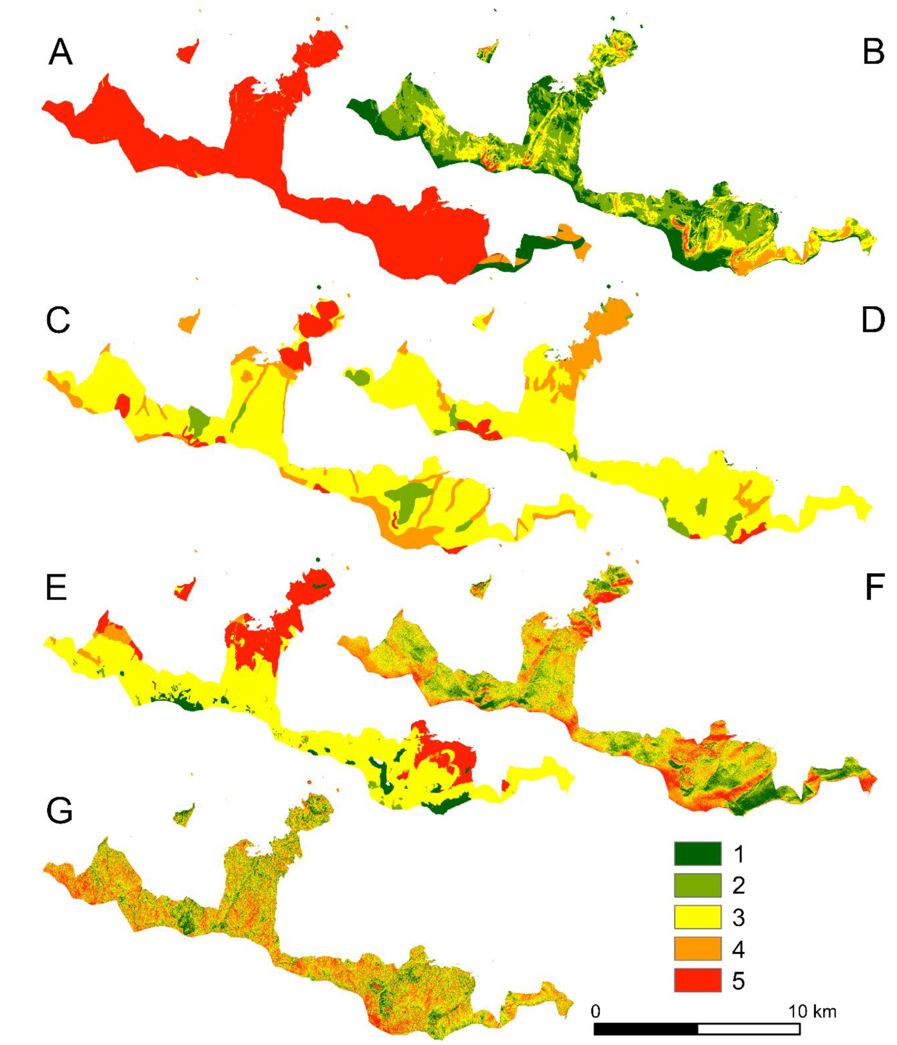
3.4. Geodiversity Assessment

The complete 57 geo-questionnaire responses provided data for 57 sets of seven aforementioned geodiversity factor maps with each factor rated on a five-point Likert scale [35]. The factor rating values were subsequently normalized to the 0.0–1.0 scale. Next, the normalized factor values were allocated to each of the 419 polygon feature catchments by calculating the area-weighted mean of raster cell values for each of the seven input factors. This step was carried out with the help of command-line open-source GRASS GIS v.7.8 [36]. The resulting 57 vector polygon layers, containing the respondents’ assessment ratings of geodiversity classes, constituted the input file for the analysis.

3.5. Multicriteria Evaluation

Two multicriteria evaluation techniques were adopted for the geodiversity assessment: weighted linear combination (WLC) [9,37] and locally weighted linear combination (L-WLC) [14]. In this study, we used the implementation of two techniques in the MCDA4ArcMap add-in [38]. MCDA4ArcMap is an open-source tool for spatial multicriteria analysis written in C# programming language within the NET environment [39]. It serves as a geovisualization tool for exploring vector GIS data and is implemented as an add-in in ArcMap. The analytical functionality of the tool includes the WLC and L-WLC method.

In both techniques, each geodiversity factor was treated as a benefit factor where the objective was to maximize the factor’s rating value. The maximum score normalization was applied in both methods (Figure 5). A major question in the case of L-WLC is the definition of neighborhood. In order to avoid the impossibility of calculating local weights due to unfortunate neighborhood arrangement resulting in zero-value local range (see Equation (1)), the extended neighborhood option (automatic neighborhood definition) was chosen in MCDA4ArcMap [40]. The tool computations resulted in 57 tables with global (WLC) and local (L-WLC) sets of factor weights that were joined with catchment layer attribute tables. In the final step of the task, two geodiversity maps were created for each respondent: (a) a geodiversity map with WLC-based geodiversity scores for each catchment area, and (b) a geodiversity map with L-WLC-based geodiversity scores for each catchment area. The geodiversity maps were obtained with a standard polygon-to-raster data conversion.

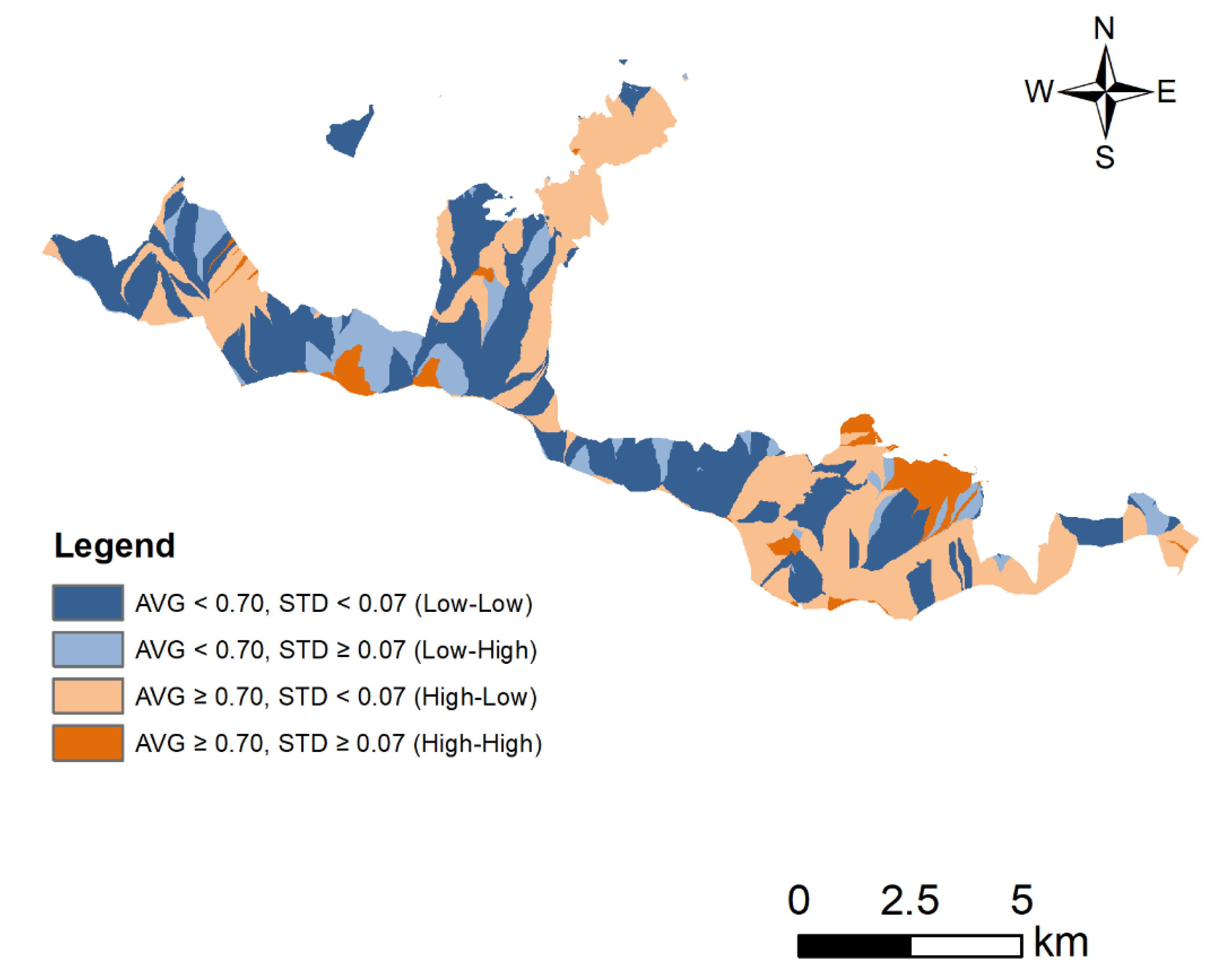
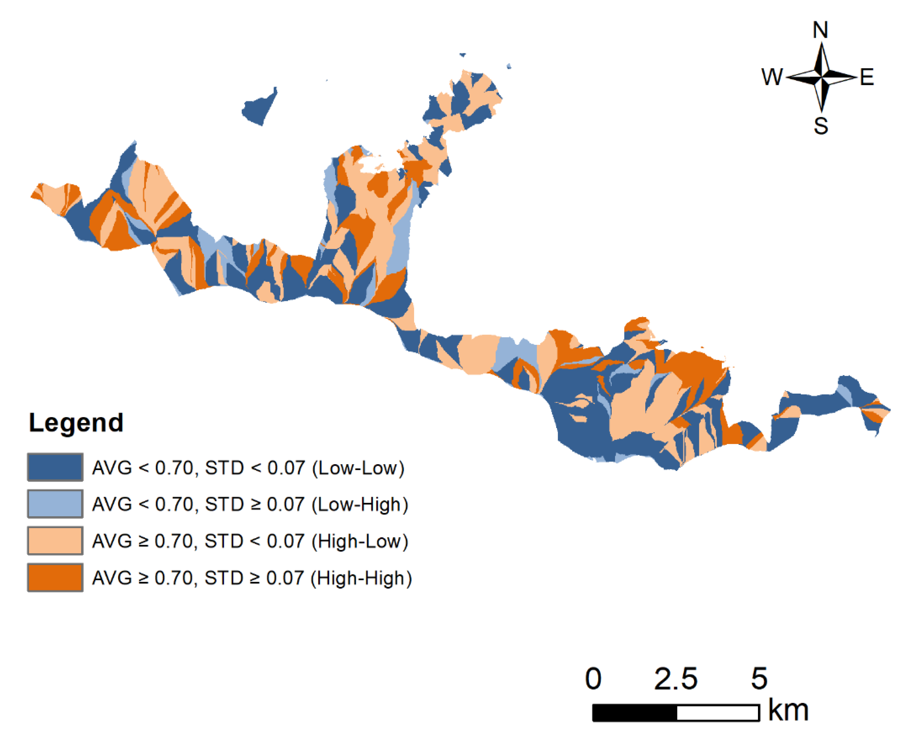
3.6. Uncertainty Analysis

The purpose of uncertainty analysis (UA) is to account for the influence of inputs on the variability (uncertainty) of model output [41]. In the study, the UA of geodiversity assessment was carried out by calculating the mean geodiversity map (the mean of 57 respondent maps) for both WLC and L-WLC, converting the floating point rasters (means) to integer rasters (integer means), and reclassifying them into two-class maps based on the average (AVG) and standard deviation (STD) values of geodiversity. For the purpose of classification, the means of both integer rasters (i.e., the mean of means and the mean of standard deviations) were adopted as threshold values. The following thresholds were used: mean AVG = 0.70 and 0.64 < AVG < 0.95; mean STD = 0.07 and 0.05 < STD < 0.22. The reclassified integer raster layers were then combined using the Map Algebra local overlay [42] into the surfaces representing the cross-tabulation of high (>0.70) and low (<0.70) AVG geodiversity, and low (<0.07) and high (>0.07) STD for both WLC and L-WLC (Figure 6 and Figure 7). The two-by-two design resulted in four classes representing four categorical outcomes for geodiversity and its uncertainty (Figure 6 and Figure 7):

(1)

Low–Low: A relative low geodiversity and low uncertainty (high confidence) areas also referred to as low–low areas. These are the areas that could be categorized as exhibiting potentially inferior geodiversity based on the classification thresholds for mean geodiversity and standard deviation.

(2)

Low–High: A relative low geodiversity and high uncertainty (low confidence) areas referred to as low–high. These areas could be considered as candidates pending further investigation of uncertainty sources, but, overall, the areas are of inferior geodiversity.

(3)

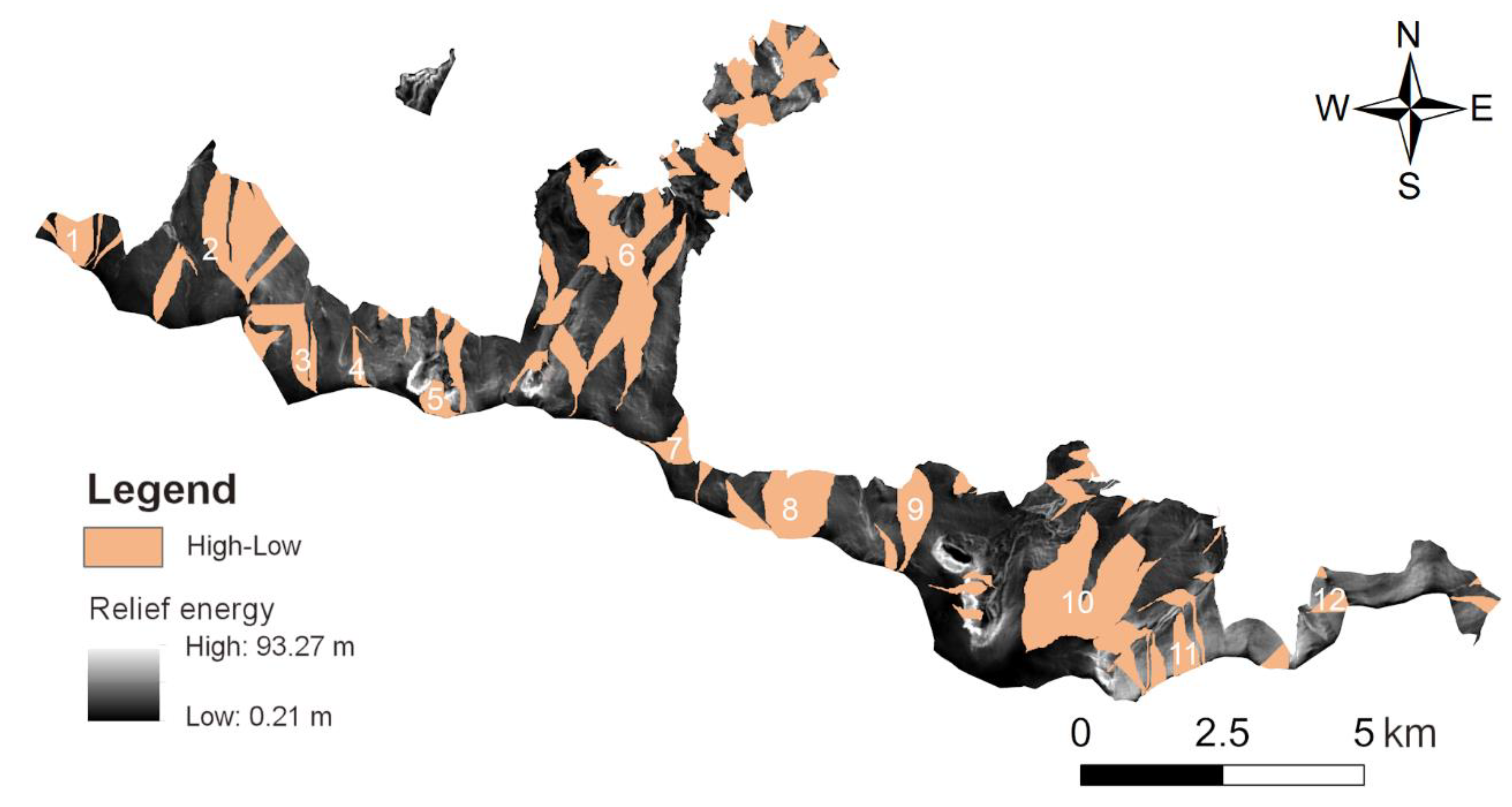
High–Low: A relative high geodiversity and low uncertainty (high confidence) areas referred to as high–low. These are robust areas that could be considered as superior geodiversity areas.

(4)

High–High: A relative high geodiversity and high uncertainty (low confidence) areas referred to as high–high. These areas could be considered as candidate for superior geodiversity areas pending further investigation of uncertainty sources.

4. Results and Discussion

The workflow (Figure 2) leads to the cross-tabulation of mean and standard deviation values (Figure 6 and Figure 7) for the geodiversity scores calculated on the bases of respondents’ ratings and weights. The geodiversity assessment in the proposed method is based on the following assumptions:

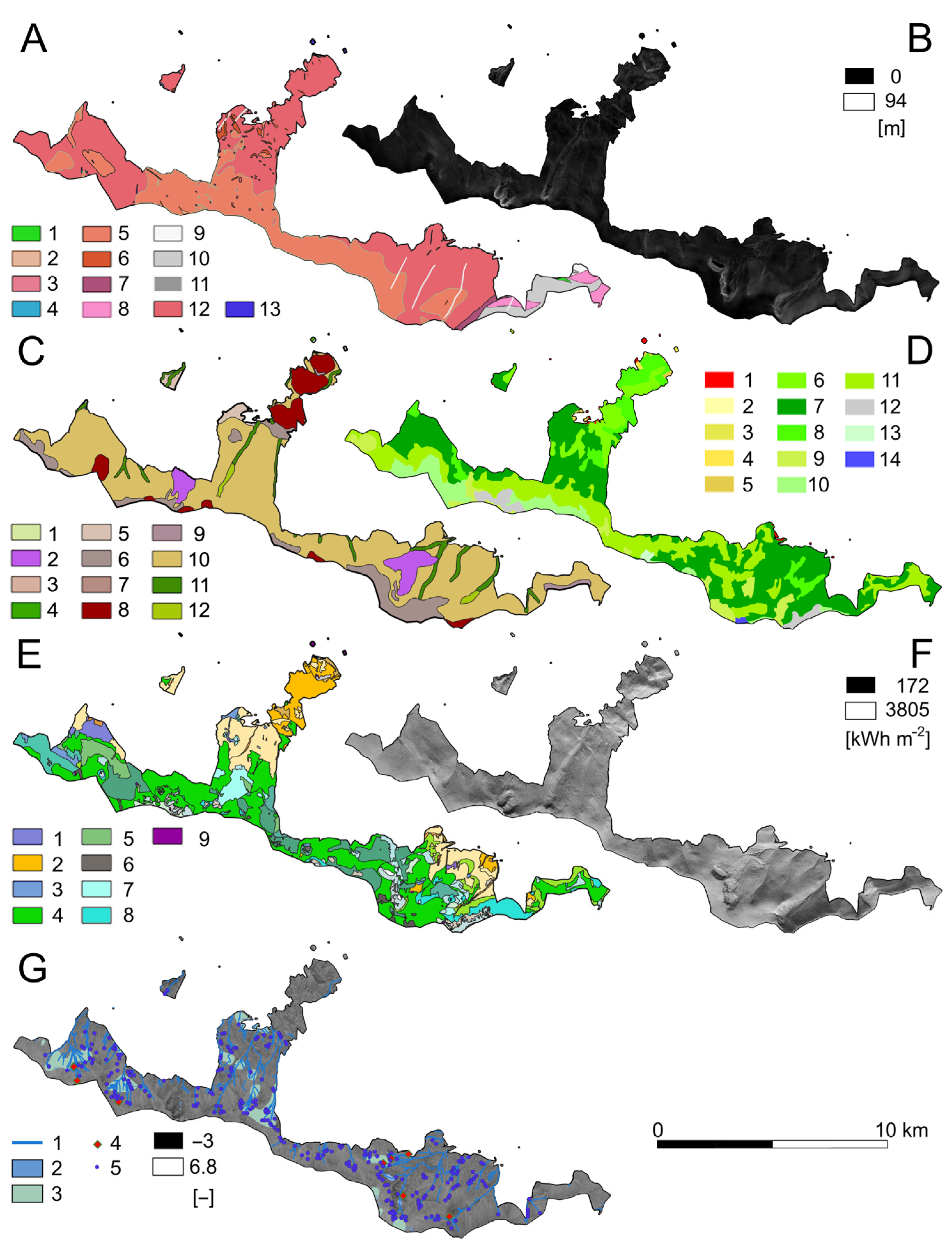
• One can identify the components of natural environment (factors) that will form the basis for factor maps in the geodiversity assessment.
• Reasonable factor ratings and weights can be crowdsourced by means of a geo-questionnaire.
• An assessment area can be logically subdivided into smaller spatial analysis units, e.g., microregions, catchments, hydrological response units etc. In this paper, catchments were selected due to the high fragmentation of the assessment area.
• Ratings of the geo-questionnaire respondents can be assigned to individual spatial units, i.e., catchments.
• Geodiversity appraisal scores are calculated with WLC and L-WLC techniques.

The above assumptions present two potential biases in the method. The first is the selection of respondents, recruited from a broad pool of specialists in various sub-disciplines in Earth sciences and environmental protection. This study included respondents with different research interests and commitments, who inadvertently might have introduced bias in data through factor ratings and weights focused in their specialty domain. The second bias stems from the selection of spatial analysis unit for geodiversity assessment. In our case, first-order catchments were selected. However, in the absence of authoritative map with detailed hydrographic divisions of the Karkonosze Mountains, the catchments were derived through the algorithmic processing of 1 m ground resolution DEM. Although the GIS algorithms for determining watershed boundaries are good, they are not perfect. Bearing in mind these two biases, one can interpret the obtained results.

The geodiversity map of the catchments obtained with the WLC technique, presented in Figure 6, shows two key features of the studied area. The largest area (25.5 km² or 42.9% of KNP area) is covered by catchments described by the low–low categories of average geodiversity (AVG) and its uncertainty (STD), which should be interpreted as predominating areas of low geodiversity accompanied by relative high confidence. These areas include, among others, the meadow beneath Mt. Łabski Szczyt in the western part of the park, the Polish Stream Valley in the central area of the park, and the Little Pond kettle in the eastern part of the park (Figure 8). The second most widely represented category pair (AVG, STD), covering the area of 23.6 km² (39.7% of KNP area), is the high–low pair representing a significant value of geodiversity accompanied by relative high confidence in the assessment. The areas in this category encompass prominent features of the park such as Mt. Szrenica in the western part of the park, Mt. Chojnik in the north-central part of the park, and Mt. Śnieżka in the eastern part of the park (Figure 8). These two category pairs represent the areas of clear geodiversity divergence between high and low values and little uncertainty. The other two category pairs, i.e., low–high and high–high, occupy only 10.3 km² or 17.3% of KPN area in total, and they should be also interpreted as the areas of clear geodiversity divergence. However, in contrast to the low–low and high–low pairs, these areas have higher uncertainty of assessment. Examples of these areas include the Snow kettles (high–high), and the foreground of the Snow kettles (low–high), both in the central section of KNP (Figure 8).

The second geodiversity map (Figure 7), calculated with the L-WLC technique, also shows (similarly to the WLC result) the low–low category occupying a significant share of park area (23.5 km² or 39.5%). However, differently to the map depicting the results of WLC technique, the areas classified as low–low are much more fragmented and dispersed. This category pair includes features such as the headwaters of the Kamieńczyk stream in the most western part of the park, and the areas surrounding the Great Pond and Little Pond in the headwaters area of the Łomnica Valley excluding the ponds (Figure 8). Interestingly enough, the next two categories, high–low and high–high, taken together occupy more than half of the park area (31 km² or 52.1%). This implies that the respondents not only highly rated the geodiversity factors for much of KNP area, but also that their ratings were amplified by the local multicriteria technique, more so than by the global technique. This may also be the results of geodiversity richness detected locally, which is higher than for the park when taken as a whole. This potential difference stems from the methodological difference between L-WLC and WLC, where the former calculates geodiversity scores for each spatial unit (i.e., catchment) based on the differences in factor ratings and weights found in local neighborhoods formed for each catchment by its neighboring catchments. That said, the aggregation of ratings and weights in the high–high category pair (11.7 km² or 19.7% of KNP area) exhibited more variance, and hence uncertainty than the high–low category pair. The areas representative of high geodiversity, according to the L-WLC results, include, among others, the Mumlawski Slope with the meadow near Kamiennik together with the Ciekotka Valley and the Złoty Potok Valley in the western part of the park, some fragments of the Wrzosówka Valley and the Polish Stream Valley in the middle section of the park, and the White Gorge and the Łomniczka kettle within the Łomniczka Valley in the eastern section of the park (Figure 8). The low–high category is characterized by the smallest area (4.9 km² or 8.2% of KNP), as for the case of WLC results. An example of the park area in this category pair is the vast northern slopes of Mt. Śnieżka covered with the hornfels boulder field.

Comparing the two maps in Figure 6 and Figure 7, the map that better reflects the degree of geodiversity of KNP is the map depicting the results of L-WLC technique (Figure 7). It contains more areas of high geodiversity value (the high–low and high–high pairs) than the WLC map (31 km² versus 27.3 km²). Given that WLC has been a previously used multicriteria approach to geodiversity assessment [7,8,31], the L-WLC technique represents an improvement over the WLC technique in its ability to capture local changes in geodiversity. Conversely, the L-WLC technique resulted in fewer low–low areas than WLC.

Table 1. Comparison of geodiversity maps resulted from WLC and L-WLC techniques from the catchment perspective.

WLC	L-WLC				Total
	Low–Low	Low–High	High–Low	High–High
Low–Low	74	16	39	23	152
Low–High	30	15	20	18	83
High–Low	54	8	49	35	146
High–High	7	13	8	10	38
Total	165	52	116	86	419

presents the numerical comparison of the category pairs resulting from WLC and L-WLC. It shows that 148 (35%) of the catchments do not change the category pair in the assessment of geodiversity. These catchments are represented by the four cells on the table’s diagonal. The catchments designated as low–low (74) and high–low (49) are the most consistent in maintaining their category designation across the results of two techniques. Conversely, 58 (14%) catchments completely changed the category designation across the results. The most numerous among them are the catchments that moved from low–low to the high–high category pair (23 catchments). The prominent features in the park that moved from low–low in WLC to high–high in L-WLC include the headwaters of the Kamienna River in the most western section of the park and the Kamieńczyk Valley—a bit further to the east, some fragments of the upper course of the Wrzosówka stream in the center part of the park, and the Upłaz. The least frequent changes concerned the transition from high–high to low–low (seven catchments), from high–low to low–high (eight catchments), and from high–high to high–low (eight catchments).

Given that L-WLC provides a realistic assessment of geodiversity and guided by its results, the following areas of high geodiversity and low uncertainty have been identified (Figure 8): 1. the Mumlawski Slope; 2. the meadow near Kamiennik with the Ciekotka Valley and the Złoty Potok Valley; 3. the Szrenickie Wetlands; 4. the Łabski kettle; 5. the Snow kettles; 6. fragments of the Wrzosówka Valley, the Polish Stream Valley, and Mt. Chojnik; 7. the headwater of the Sopot Valley; 8. the northern slopes of Mt. Mały Szyszak; 9. the northern slopes of Mt. Smogornia; 10. the White Gorge and the Łomniczka kettle with the Łomniczka Valley; 11. the northern slopes of the Black Ridge; and 12. the western slopes of Mt. Rock Table. Each of these areas is located on the northern slopes of the Karkonosze Mountains and is undoubtedly an interesting geological, geomorphological, sometimes hydrographic and biogenic peculiarity [27]. However, it should be noted that the areas of the plain beneath Mt. Śnieżka with the Upy peat bog, the Great Pond and the Little Pond kettles, Mt. Łabski Szczyt and Mt. Szrenica were not classified among the areas of significant geodiversity. Arguably, these areas could be considered as candidates for the high–low category.

5. Conclusions

Geodiversity is essential to human well-being and provides the foundations and habitats for all living things [31,43]. It offers the evidence of past climate and landscape changes and their causes and consequently helps to understand and plan for the impacts of future environmental changes. As such, geodiversity is crucial in promoting sustainable use of the Earth’s resources and geo-ecosystem services. That being said, societies tend to value what is measured; thus, there is a need to develop geodiversity valuation methods that introduce a degree of guidance and rigor in data interpretation and assessment.

In this paper, one approach to measuring geodiversity and the uncertainty of measurement has been presented. The approach builds on the WLC-based assessment method in two distinct ways. First, it employs a crowdsourcing approach to collect the geodiversity factor ratings and weights pertaining to a specific assessment area (i.e., KNP). Second, it extends the WLC-based assessment by adding a local spatial multicriteria analysis technique (L-WLC) and averaging the geodiversity assessments on the individual response basis (the geo-questionnaire respondents). Thus, an average geodiversity assessment score is computed for each spatial analysis unit (i.e., the first-order catchment polygon) and, thus, is the standard deviation value representing the uncertainty of average geodiversity score. Next, the distributions of average and standard deviation values are examined for salient data points (e.g., distribution mean or data frequency break-point), which serve as guidelines for threshold values. The thresholds are used to compile a bivariate map with average geodiversity values (AVG: low, high) and standard deviation values (STD: low, high). Two such maps, one for WLC results and another for L-WLC results, are compiled and evaluated, providing a more holistic picture of average geodiversity and its uncertainty.

The presented approach could be extended further in the following ways: Differences between the solutions could be investigated by focusing on specific neighborhoods in a study area or a sample of randomly selected neighborhoods and comparing the geodiversity scores computed with WLC and L-WLC for each spatial unit. In another extension, the uncertainty of assessment could be investigated by way of spatially explicit global sensitivity analysis [41] aimed at discovering influential input factors (i.e., ratings and weights) that contribute the most to uncertainty of assessment, and locations within the study area where the influence is the strongest. It is also worth to consider the uncertainty analysis of respondents’ assessments for individual geodiversity factors and components. Last, but not least, the efficacy of presented approach could be further investigated by extending it to other physiographic and climatic landscapes, including uplands and lowlands, as well as choosing other spatial analysis methods, such as microregions and/or hydrological response units. This might offer evidence for or against the efficacy of the presented approach for areas and landscapes other than that used in this study. That being stated, the presented approach still relies on the area-specific assessment of a contribution made by each geodiversity factor to the overall measure of geodiversity, which means that there are limits to generalizing an assessment made for one area to other areas.

References

1. Sharples, C. Geoconservation in forest management—Principles and procedures. Tasforests 1995, 7, 37–50. [Google Scholar]
2. Gray, M. Geodiversity: Valuing and Conserving Abiotic Nature, 2nd ed.; John Wiley & Sons Ltd.: Chichester, UK, 2013; ISBN 978-0-470-74215-0. [Google Scholar]
3. Gray, M. Geodiversity: Valuing and Conserving Abiotic Nature; Wiley: Chichester, UK, 2004; ISBN 0-470-84895-2. [Google Scholar]
4. Zwoliński, Z. Geodiversity. In Encyclopedia of Geomorphology; Goudie, A.S., Ed.; Routledge: London, UK, 2004; Volume 1, pp. 417–418. [Google Scholar]
5. Coratza, P.; Reynard, E.; Zwoliński, Z. Geodiversity and Geoheritage: Crossing Disciplines and Approaches. Geoheritage 2018, 10, 525–526. [Google Scholar] [CrossRef] [Green Version]
6. Barron, H.; Gordon, J.E. The role of geodiversity in delivering ecosystem services and benefits in Scotland. Scott. J. Geol. 2013, 49, 41–58. [Google Scholar] [CrossRef] [Green Version]
7. Zwoliński, Z.; Najwer, A.; Giardino, M. Methods for Assessing Geodiversity. In Geoheritage: Assessment, Protection, and Management; Reynard, E., Brilha, J., Eds.; Elsevier: Amsterdam, The Netherlands, 2018; pp. 27–52. [Google Scholar] [CrossRef]
8. Najwer, A.; Borysiak, J.; Gudowicz, J.; Mazurek, M.; Zwoliński, Z. Geodiversity and Biodiversity of the Postglacial Landscape (Dębnica River Catchment, Poland). Quaest. Geogr. 2016, 35, 5–28. [Google Scholar] [CrossRef] [Green Version]
9. Malczewski, J.; Rinner, C. Multi-Criteria Decision Analysis in Geographic Information Science; Springer: Berlin/Heidelberg, Germany, 2015. [Google Scholar] [CrossRef]
10. Zwoliński, Z. The routine of landform geodiversity map design for the Polish Carpathian Mts. Landf. Anal. 2009, 11, 77–85. [Google Scholar]
11. Zwoliński, Z.; Stachowiak, J. Geodiversity map of the Tatra National Park for geotourism. Quaest. Geogr. 2012, 31, 99–107. [Google Scholar] [CrossRef] [Green Version]
12. Becker, W.; Saisana, M.; Paruolo, P.; Vandecasteele, I. Weights and importance in composite indicators: Closing the gap. Ecol. Indic. 2017, 80, 12–22. [Google Scholar] [CrossRef]
13. Malczewski, J. GIS-based multi-criteria decision analysis: A survey of the literature. Int. J. Geogr. Inf. Sci. 2006, 20, 703–726. [Google Scholar] [CrossRef]
14. Malczewski, J. Local weighted linear combination. Trans. GIS 2011, 15, 439–455. [Google Scholar] [CrossRef]
15. Czepkiewicz, M.; Jankowski, P.; Młodkowski, M. Geo-questionnaires in urban planning: Recruitment methods, participant engagement, and data quality. Cartogr. Geogr. Inf. Sci. 2017, 44, 551–567. [Google Scholar] [CrossRef]
16. Jankowski, P.; Czepkiewicz, M.; Młodkowski, M.; Zwoliński, Z. Geo-questionnaire: A Method and Tool for Public Preference Elicitation in Land Use Planning. Trans. GIS 2016, 20, 903–924. [Google Scholar] [CrossRef]
17. See, L.; Mooney, P.; Foody, G.; Bastin, L.; Comber, A.; Estima, J.; Fritz, S.; Kerle, N.; Jiang, B.; Laakso, M.; et al. Crowdsourcing, Citizen Science or Volunteered Geographic Information? The Current State of Crowdsourced Geographic Information. ISPRS Int. J. Geo-Inf. 2016, 5, 55. [Google Scholar] [CrossRef]
18. Surowiecki, J. The Wisdom of Crowds; Doubleday: New York, NY, USA, 2004. [Google Scholar]
19. Aristotle. Politics; Rackham, H., Ed.; Harvard University Press: Cambridge, UK, 1932; ISBN 9780674992917. [Google Scholar]
20. Czepkiewicz, M.; Brudka, C.; Jankowski, P.; Kaczmarek, T.; Zwoliński, Z.; Mikuła, Ł.; Bąkowska, E.; Młodkowski, M.; Wójcicki, M. Public Participation GIS for sustainable urban mobility planning: Methods, applications and challenges. Rozw. Reg. i Polityka Reg. 2016, 35, 9–35. [Google Scholar]
21. Kahila, M.; Kyttä, M. SoftGIS as a bridge-builder in collaborative urban planning. In Planning Support Systems Best Practice and New Methods; Geertman, S., Stillwell, J., Eds.; Springer: Berlin/Heidelberg, Germany, 2009; pp. 389–411. [Google Scholar] [CrossRef]
22. Brown, G.; Weber, D. Public Participation GIS: A new method for national park planning. Landsc. Urban Plan. 2011, 102, 1–15. [Google Scholar] [CrossRef]
23. Chaix, B.; Kestens, Y.; Perchoux, C. An interactive mapping tool to assess individual mobility patterns in neighborhood studies. Am. J. Prev. Med. 2012, 43, 440–450. [Google Scholar] [CrossRef] [Green Version]
24. Jankowski, P.; Czepkiewicz, M.; Młodkowski, M.; Zwoliński, Z.; Wójcicki, M. Evaluating the scalability of public participation in urban land use planning: A comparison of Geoweb methods with face-to-face meetings. Environ. Plan. B Urban Anal. City Sci. 2019, 46, 511–533. [Google Scholar] [CrossRef]
25. Haklay, M.; Jankowski, P.; Zwoliński, Z. Selected modern methods and tools for public participation in urban planning—A review. Quaest. Geogr. 2018, 37, 127–149. [Google Scholar] [CrossRef] [Green Version]
26. Fischer, G.W. Range sensitivity of attribute weights in multiattribute value models. Organ. Behav. Hum. Decis. Process. 1995, 62, 252–266. [Google Scholar] [CrossRef]
27. Knapik, R.; Migoń, P. Atlas. Georóżnorodność i Geoturystyczne Atrakcje Karkonoskiego Parku Narodowego i Otuliny; Karkonoski Park Narodowy: Jelenia Góra, Poland, 2011; pp. 1–100. ISBN 978-83-933795-8-3. [Google Scholar]
28. KNP (Karkonosze National Park). Dane GIS z terenu KNP; Jelenia Góra, 2019; Umowa nr GIS/4/2019 z dn. 16.04.2019. [Google Scholar]
29. CLC (CORINE Land Cover). Projekt Corine Land Cover 2018 w Polsce; Główny Inspektorat Ochrony Środowiska: Warszawa, Poland, 2020. Available online: https://clc.gios.gov.pl (accessed on 26 October 2020).
30. ESRI (Environmental Systems Research Institute). Arc Hydro Tools 2.0—Facilitate the Creation, Manipulation, and Display of Arc Hydro Features; Informer Technologies, Inc.: California, CA, USA, 2020; Available online: https://arc-hydro-tools.software.informer.com/2.0/ (accessed on 26 October 2020).
31. Najwer, A.; Zwoliński, Z. Semantyka i metodyka oceny georóżnorodności—Przegląd i propozycja badawcza. Landf. Anal. 2014, 26, 115–127. [Google Scholar] [CrossRef]
32. Crofts, R.; Gordon, J.E.; Brilha, J.; Gray, M.; Gunn, J.; Larwood, J.; Santucci, V.L.; Tormey, D.; Worboys, G.L. Guidelines for Geoconservation in Protected and Conserved Areas; Best Practice Protected Area Guidelines Series No. 31; IUCN: Gland, Switzerland, 2020. [Google Scholar] [CrossRef]
33. GeoServer Development Team. GeoServer Software; Open Source Geospatial Foundation: Chicago, IL, USA, 2020; Available online: http://geoserver.org (accessed on 26 October 2020).
34. Recoded GitLab. Geoankieta. 2020. Available online: https://recoded.co/geoplan/geoankieta (accessed on 26 October 2020).
35. Likert, R. A Technique for the Measurement of Attitudes. Arch. Psychol. 1932, 140, 1–55. [Google Scholar]
36. GRASS Development Team. Geographic Resources Analysis Support System (GRASS) Software; Open Source Geospatial Foundation: Chicago, IL, USA, 2020; Available online: http://grass.osgeo.org (accessed on 26 October 2020).
37. Hopkins, L. Methods for generating land suitability maps: A comparative evaluation. J. Am. Inst. Plan. 1977, 34, 19–29. [Google Scholar] [CrossRef]
38. Rinner, C.; Voss, S. MCDA4ArcMap: An open-source multi-criteria decision analysis and geovisualization tool for ArcGIS 10. Cartouche 2013, 86, 12–13. [Google Scholar]
39. Voss, S. MCDA4ArcMap 1.1A for ArcMap 10.2 or Later rev36981. 2020. Available online: https://github.com/steffanv/mcda4arcmap/releases/tag/1.1Anew (accessed on 26 October 2020).
40. Voss, S. MCDA4ArcMap version 1.1A. 2020. Available online: https://github.com/steffanv/mcda4arcmap/releases/download/1.1Anew/MCDA4ArcMap.User.Guide.pdf (accessed on 26 October 2020).
41. Ligmann-Zielinska, A.; Jankowski, P. Spatially-explicit integrated uncertainty and sensitivity analysis of criteria weights in multicriteria land suitability evaluation. Environ. Model Softw. 2014, 57, 235–247. [Google Scholar] [CrossRef]
42. Tomlin, C.D. Geographical Information Systems and Cartographic Modeling; Prentice-Hall: Englewood Cliffs, NJ, USA, 1990. [Google Scholar]
43. Hjort, J.; Gordon, J.E.; Gray, M.; Hunter, M.L., Jr. Why geodiversity matters in valuing nature’s stage. Conserv. Biol. 2015, 29, 630–639. [Google Scholar] [CrossRef]
Figure 1. Digital Elevation Model of the Karkonosze National Park (KNP).
Ijgi 09 00716 g001
Figure 2. Data processing workflow.
Ijgi 09 00716 g002
Figure 3. Input dataset of environmental components for geodiversity assessment. (A) lithology: 1—amphibolite, 2—aplite, 3—basaltoid, basanite, 4—cataclasite, mylonite, tectonic breccia, 5—equigranular granite, 6—fine-grained granite, 7—hornfels, 8—laminated augen gneiss, 9—leptynite, 10—mica schist, 11—microgranite, 12—porphyritic granite, 13—vein quartz; (B) relief energy (relative height): from 0 to 94 m; (C) geomorphology: 1—floodplain, 2—hillock moraine, 3—intramontane basin, 4—meadow terraces, 5—planation surface in basin bottom, 6—planation surface on flat-topped hill, 7—planation surface on slope, 8—residual hill—resistance monadnock, 9—rock wall or rock slope, 10—slope, 11—V-shaped valley, 12—valley bottom with moraine cover; (D) land cover and land use: 1—discontinuous urban fabric, 2—non-irrigated arable land, 3—pastures, 4—complex cultivation patterns, 5—agricultural land with areas of natural vegetation, 6—broad-leaved forest, 7—coniferous forest, 8—mixed forest, 9—natural grasslands, 10—moors and heathland, 12—transitional woodland shrub, 13—bare rocks, 14—sparsely vegetated areas, 15—peat bogs; (E) soils: 1—Endogleyic Cambisols, 2—Haplic Cambisols, 3—Haplic Fluvisols, 4—Haplic Podzol, 5—Haplic Regosols, 6—Histosols, 7—Leptic Regosols, 8—Leptosols, 9—Urbic Technosols; (F) solar irradiance: from 172 to 3805 kWh m−2; (G) hydrography: 1—rivers and streams, 2—lakes, ponds, reservoirs, 3—wetlands and swamps larger than 10 ha, 4—wetlands and swamps smaller than 10 ha, 5—springs, topographic wetness index: from −3.0 to 6.8 [–]. Data sources are listed in the text.
Ijgi 09 00716 g003
Figure 4. Geo-questionnaire application for Karkonosze National Park (KNP); page 3 with the relief energy geodiversity factor. On this page, a respondent is asked to select one of three classifications representing three possible geodiversity ratings of relief energy (a derivative of local elevation change).
Ijgi 09 00716 g004
Figure 5. Factor maps of partial lithological (A); relief energy (B); geomorphological (C); land cover and land use (D); soil (E); solar irradiance (F); and hydrographical (G) geodiversity normalized to five classes: 1—very low, 2—low, 3—medium, 4—high, and 5—very high geodiversity.
Ijgi 09 00716 g005
Figure 6. Geodiversity classification based on average geodiversity (AVG) and standard deviation (STD) for Karkonosze National Park. Geodiversity was computed using the weighted linear combination (WLC) aggregation technique for each geo-questionnaire respondent (57 in total). AVG and STD values are normalized to the 0–1 value range.
Ijgi 09 00716 g006
Figure 7. Geodiversity classification based on average geodiversity (AVG) and standard deviation (STD) for Karkonosze National Park. Geodiversity was computed using the local weighted linear combination (L-WLC) aggregation technique for each geo-questionnaire respondent (57 in total). AVG and STD values are normalized to 0–1 value range.
Ijgi 09 00716 g007
Figure 8. Areas of high geodiversity and low uncertainty (high–low calculated with the L-WLC technique) on the background of relief energy map (relative height). Digits 1–12 denote the selected features of KNP referred to in the Results and Discussion Section: 1. the Mumlawski Slope; 2. the meadow near Kamiennik with the Ciekotka Valley and the Złoty Potok Valley; 3. the Szrenickie Wetlands; 4. the Łabski kettle; 5. the Snow kettles; 6. fragments of the Wrzosówka Valley, the Polish Stream Valley and Mt. Chojnik; 7. the headwater of the Sopot Valley; 8. the northern slopes of Mt. Mały Szyszak; 9. the northern slopes of Mt. Smogornia; 10. the White Gorge and the Łomniczka kettle with the Łomniczka Valley; 11. the northern slopes of the Black Ridge; and 12. the western slopes of Mt. Rock Table.
Ijgi 09 00716 g008