Spatiotemporal LUCC Simulation under Different RCP Scenarios Based on the BPNN_CA_Markov Model: A Case Study of Bamboo Forest in Anji County

Abstract

Simulating spatiotemporal land use and land cover change (LUCC) data precisely under future climate scenarios is an important basis for revealing the carbon cycle response of forest ecosystems to LUCC. In this paper, a coupling model consisting of a back propagation neural network (BPNN), Markov chain, and cellular automata (CA) was designed to simulate the LUCC in Anji County, Zhejiang Province, under four climate scenarios (Representative Concentration Pathway (RCP) 2.6, 4.5, 6.0, 8.5) from 2024 to 2049 and to analyze the temporal and spatial distribution of bamboo forests in Anji County. Our results provide four outcomes. (1) The transition probability matrices indicate that the area of bamboo forests shows an expansion trend, and the largest contribution to the expansion of bamboo forests is the cultivated land. The Markov chain composed of the average transition probability matrix could perform excellently, with only small errors when simulating the areas of different land-use types. (2) Based on the optimized BPNN, which had a strong generalization ability, a high prediction accuracy, and area under the curve (AUC) values above 0.9, we could obtain highly reliable land suitability probabilities. After introducing more driving factors related to bamboo forests, the prediction of bamboo forest changes will be more accurate. (3) The BPNN_CA_Markov coupling model could achieve high-precision simulation of LUCC at different times, with an overall accuracy greater than 70%, and the consistency of the LUCC simulation from one time to another also had good performance, with a figure of merit (FOM) of approximately 40%. (4) Under the future four RCP scenarios, bamboo forest evolution had similar spatial characteristics; that is, bamboo forests were projected to expand in the northeast, south, and southwest mountainous areas of Anji County, while bamboo forests were projected to decline mainly around the junction of the central and mountainous areas of Anji County. Comparing the simulation results of different scenarios demonstrates that 74% of the spatiotemporal evolution of bamboo forests will be influenced by the interactions and competition among different land-use types and other driving factors, and 26% will come from different climate scenarios, among which the RCP8.5 scenario will have the greatest impact on the bamboo forest area and spatiotemporal evolution, while the RCP2.6 scenario will have the smallest impact. In short, this study proposes effective methods and ideas for LUCC simulation in the context of climate change and provides accurate data support for analyzing the impact of LUCC on the carbon cycle of bamboo forests.

1. Introduction

Land use and land cover change (LUCC) is a direct driving factor affecting the carbon balance of terrestrial ecosystems, and its impact on global warming is second only to that of fossil fuels and industrial emissions [1,2,3]. The Fifth Assessment Report (AR5) produced by the Intergovernmental Panel on Climate Change (IPCC) further noted that the emissions caused by forest reduction and land-use changes are as high as 180 billion tons of carbon, accounting for 33% of the cumulative anthropogenic CO₂ emissions. Therefore, the role of land-use plans such as reforestation in mitigating climate change has been widely recognized [4]. However, the impact of climate change and LUCC on the temporal and spatial dynamics of forests has also received attention [5]. Limited LUCC data cause considerable underestimations regarding the impact of LUCC on carbon emissions [6]. The lack of spatiotemporal LUCC data under the background of the future climate is an important limitation we must overcome if we are to reveal the response of the carbon cycle of forest ecosystems to future climate change. Therefore, simulating spatiotemporal LUCC data accurately under future climate scenarios and probing the spatial evolution trajectories of LUCC has important scientific significance for revealing the response of the forest ecosystem carbon cycle to LUCC. Accurate LUCC simulation is proposed under the background that LUCC affects the carbon budget of terrestrial ecosystems, and global climate change has an urgent need for information on the regional and global future land-use spatiotemporal evolution patterns [7].

At present, spatiotemporal LUCC simulation mainly includes the simulation of quantity changes and spatial distribution changes. There are many models for these two situations, and these models can be roughly divided into three types: quantitative models, spatial models, and coupling models of quantitative and spatial models. Quantitative models focus on the analysis of the area change and rate of change of each land-use type, including the gray correlation, Markov chain, logistic regression, and system dynamic models [8,9,10]. Gobin et al. [11] used a logistic regression model to predict the quantity of agricultural land in southeastern Nigeria. Tian et al. [12] projected China’s land-use demand under different scenarios from 2010 to 2050 based on the system dynamic model. Spatial models that mainly include the cellular automata (CA) model, the conversion of land use and its effects at small regional extent (CLUE-S) model and Geomod model, combine remote sensing and geographic information system technology to overcome the shortcomings of quantitative models regarding the spatial scale, and could be used to reveal the LUCC and its interrelationships on different temporal and spatial scales [13,14,15,16]. However, the efficiency of some spatial models, such as the CLUE-S model, is not satisfactory because the model must rely on relevant results provided by quantitative models to make reasonable predictions for various land-use types [17,18].

The single model described above does not fully consider the internal mechanism of the ecosystem when simulating LUCC. Therefore, to improve the accuracy of the simulation, the coupling of the quantitative model and the spatial model has become a popular method for accurately predicting the spatiotemporal pattern of LUCC [19]. The research results of Leemans et al. and Meijl et al. [20,21] both indicate that the coupled model is more advantageous in simulating the state of LUCC under different scenarios. Meanwhile, the CA and the Markov chain coupling model (CA_Markov) are found to be the most universal and effective models in predicting future LUCC dynamics under various scenarios [22,23,24,25]. Wu et al. [5] simulated forest landscape dynamics of Taihe County by integrating CA_Markov and a forest landscape model for 2010 to 2050. Zhao et al. [26] linked the CA_Markov and Invest models to effectively assess the potential effects of ecological engineering on carbon storage. In these studies, the Markov chain model controls the area change between land-use types by the transition probability matrix [27]. The CA model controls the spatial pattern changes by considering factors such as land suitability and neighborhood effects; thus, the use of appropriate methods to determine land suitability is also one of the keys to LUCC simulation [28]. With the development of artificial intelligence, the combination of artificial neural networks and CA models to determine land suitability and simulate the temporal and spatial evolution of land use has attracted increasing attention [7,13,29]. 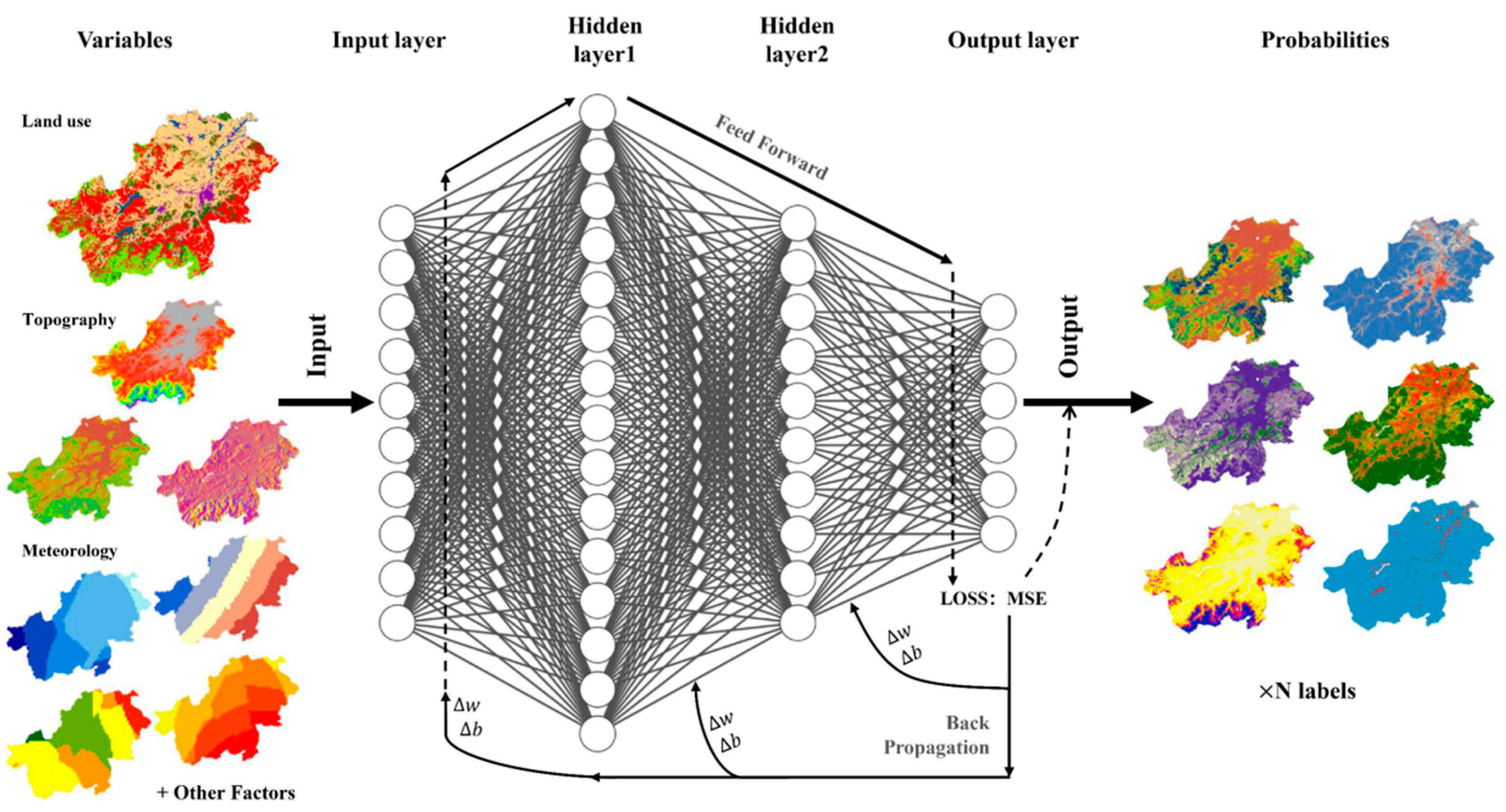A future land-use simulation (FLUS) consisting of an artificial neural network and CA model could be applied to the effective LUCC prediction of four scenarios from 2010 to 2050 that depict different development strategies by considering various socioeconomic and natural climatic factors [7]. Considering that the performance of the back propagation neural network (BPNN) is better than some artificial neural networks, the CA model integrated with the BPNN (BPNN_CA) can be designed to control the spatial pattern changes more precisely.

Global forests are under tremendous pressure from various natural and anthropogenic disturbances [30,31] that have resulted in forest loss and degradation over the past 20 years [5,32]. As efficient and reproducible tools, spatiotemporal LUCC simulations can analyze both the origins and consequences of future landscape dynamics relative to anthropogenic and natural environmental driving forces [33,34]. The complex structure of linkages and feedback will be assessed by using simulation models to predict future LUCC trajectories [35,36]. Bamboo forest is a special type of forest in the subtropical zone that has a high-efficiency carbon sequestration capacity and a strong carbon sink potential. Currently, the bamboo forest area in China, which is a veritable “world bamboo kingdom”, has reached more than 6.41 million hectares, accounting for approximately 20% of the world’s bamboo forest area; thus, it has played an important role in how regional forests respond to climate change [37]. The area of bamboo forests in China has grown at an alarming rate, with an increase of approximately 52% in the past 20 years. Furthermore, the potential suitable areas for bamboo forests in China show range contractions towards interior China and expansions towards southwestern China under future climate scenarios [38]. However, due to the unclear relationship between bamboo forests and other land-use types under the current climate change background, exploring the spatiotemporal evolution of bamboo forests under the background to grasp the competitive relationship between bamboo forests and other land-use types under the LUCC driving forces has important scientific significance for bamboo forests in terms of how they adapt to climate change and how we evaluate its contribution to the carbon balance of regional ecosystems.

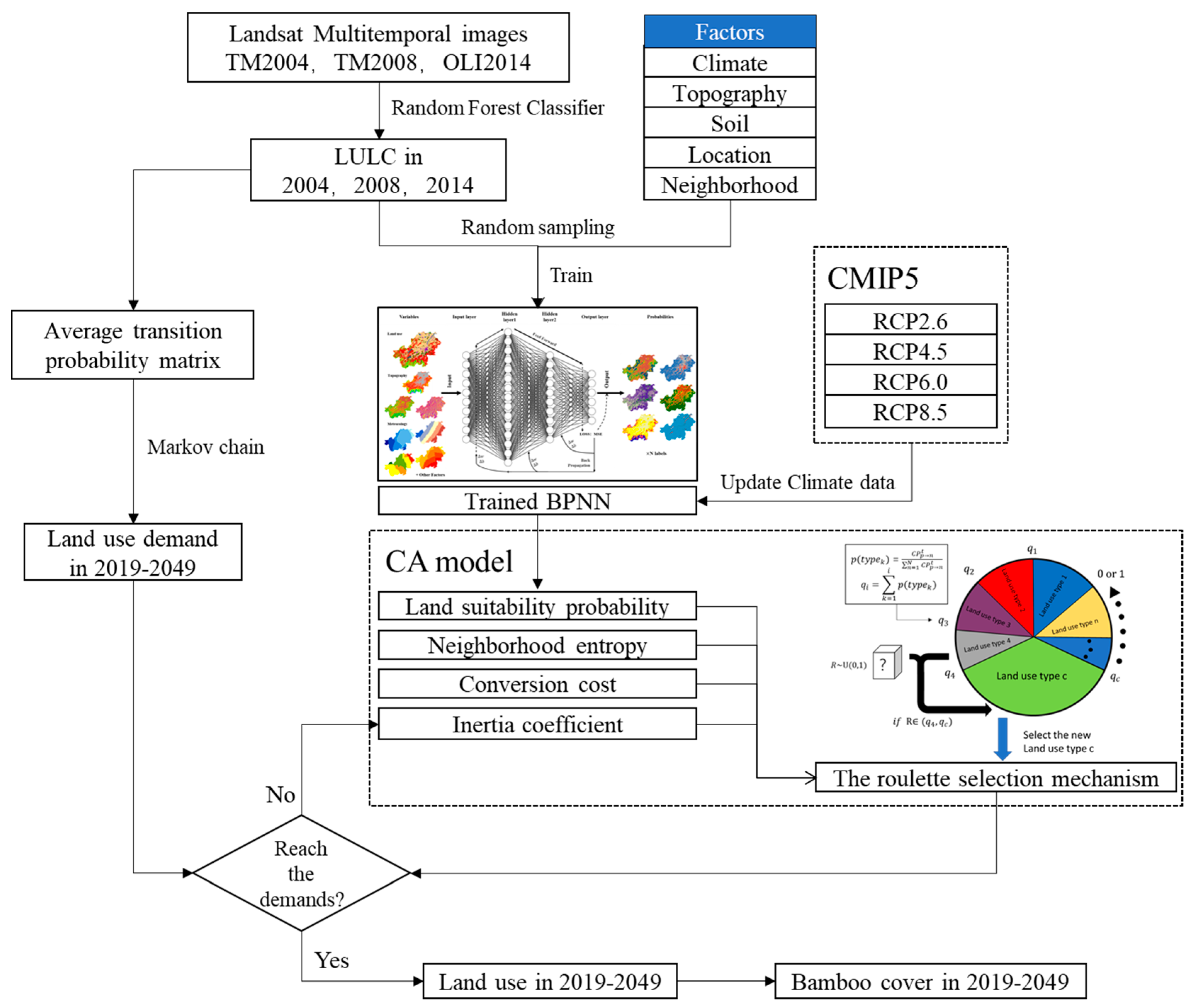
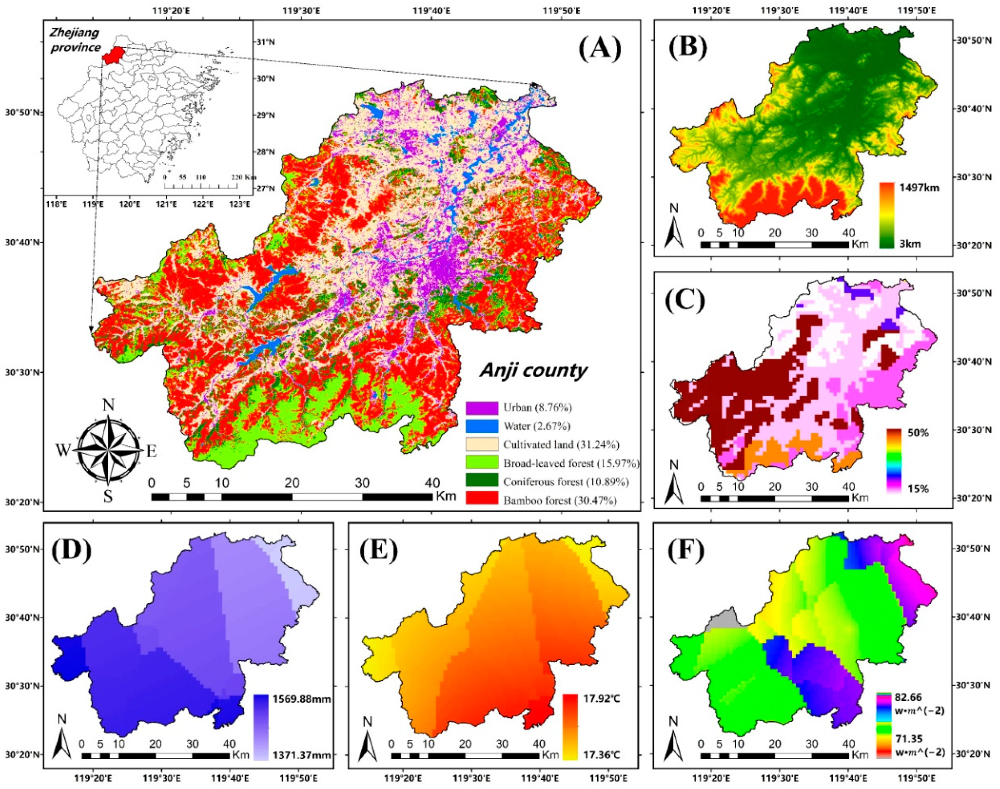
Anji County is the famous bamboo hometown of Zhejiang Province in China. In recent years, the area of bamboo forests in the county has continued to increase, and its impacts on forest types and carbon cycles have been a concern [39,40]. Therefore, based on past and current remote sensing information, this study takes Anji County as an example and uses the BPNN_CA_Markov coupling model to simulate the LUCC under the Representative Concentration Pathway (RCP) 2.6, 4.5, 6.0, and 8.5 (RCP2.6, 4.5, 6.0, 8.5) scenarios from 2024 to 2049. The objectives of our research are mainly as follows: (1) to build a Markov chain model to predict the land-use demand in the study area in a certain future period; (2) to construct a BPNN_CA model to deal with the complex competition and internal interactions between different land-use types to simulate the LUCC spatial patterns; (3) to couple the BPNN_CA model with the Markov model to simulate the spatial distribution map of land-use types that meet the quantitative demands. (4) to analyze the LUCC of Anji County under the background of climate change and reveal the impact of future climate change on the distribution of bamboo forests.

2. Materials and Methods

2.1. Study Area

Anji County is located in northwest Zhejiang Province in China, ranging from 119°14′ E to 119°35′ E and from 30°23′ N to 30°53′ N (Figure 1A). The county has a total population of 470,700 and a gross domestic product of 40.43 billion yuan in 2018. It is surrounded by mountains on three sides, with a valley bottom plain in the middle. The terrain is high in the southwest and low in the northeast (Figure 1B). Its main drainage system is Xitiao River. Its climate is subtropical maritime monsoon. Data from 2014 showed that the annual total precipitation was 1370–1570 mm (Figure 1D), the annual average temperature was 17–18 °C (Figure 1E), and the annual average radiation reached 70–83 $\mathrm{W}·{\mathrm{m}}^{-2}$ (Figure 1F), indicating sufficient sunlight, mild climate, abundant rainfall, and four distinct seasons. The soil types are mainly red soil, yellow soil, and lithological soil, among which red soil with a clay fraction of more than 40% has the largest area (Figure 1C). Anji County is rich in bamboo, covering an area of more than 60,000 hectares, accounting for more than 30% of the county’s area and more than 50% of the county’s forest area (Figure 1A).

2.2. Data

According to a review of common factors involved in LUCC modeling summarized in Poelmans [41] and Dubovyk [42], two types of driving factors are expected to explain LUCC, namely, natural environmental factors and socioeconomic factors. Based on these two types, the relevant data in

Table 1. List of data used in this study.

Category	Data	Year	Data Resource
Land use	Land-use data	2004, 2008, 2014	Based on the Landsat TM and OLI
Neighborhood effects	Urban land density	2004, 2008, 2014	Density of the specific land-use type in the Moore neighborhood
	Water body density
	Cultivated land density
	Broadleaf forest density
	Coniferous forest density
	Bamboo density
Climate	Annual total Precipitation (Pre)	2004–2014	Interpolation based on data from 410 weather stations in Zhejiang Province and its surrounding provinces, from 2004 to 2014
	Annual average radiation (Rad)
	Annual average relative humidity (Rhu)
	Annual average temperature (Tav)
Future Climate	RCP2.6 (Pre, Rad, Rhu, Tav)	2019–2049	Derived from BCC-CSM1-1 climate change modeling data
	RCP4.5 (Pre, Rad, Rhu, Tav)
	RCP6.0 (Pre, Rad, Rhu, Tav)
	RCP8.5 (Pre, Rad, Rhu, Tav)
Topography	DEM	2014	Calculated from DEM
	Slope
	Aspect
Soil	Silt fraction	2008	Derived from the Harmonized World Soil Database (HWSD 1.2)
	Clay fraction
	Wilt point
	Soil available water content
	Soil bulk density
Location	Distance to road	2014	Generated using the distance analysis function in ArcGIS 10.4
	Distance to water

were collected and processed, mainly including historical and current land-use patterns and their corresponding neighborhood effects, historical and current climate data, future climate data simulated by Coupled Model Intercomparison Project Phase 5 models, topographic conditions, soil data, road network data, and water system data.

Land-use patterns in Anji County were based on the 30 m multispectral data of Landsat-5 TM (2004, 2008) and Landsat-8 OLI (2014). After radiation correction and atmospheric correction, we used the random forest algorithm combined with the spectral band, vegetation indices, and texture variables to obtain land-use classification. Land use in this paper was classified into six types: bamboo forest (BF), broad-leaved forest (BLF), coniferous forest (CF), urban land (UL), cultivated land (CL), and water body (WB). Based on the results of the field surveys in 2004, 2008, 2014 combined with the methods of visual interpretation of high-resolution image data such as Google Earth, we obtained 366 verification plots in 2004, 435 plots in 2008, and 434 plots in 2014, respectively. These plots were used to build confusion matrices to evaluate the accuracy of the classification results. The confusion matrices for each year are shown in the

Table 2. The confusion matrices of the land-use classification in 2004, 2008, and 2014.

Year	Type	UL	WB	CL	BLF	CF	BF	OA	Kappa
2004	UL	82	1	1	0	0	0	0.9621	0.9541
	WB	1	52	0	0	0	0
	CL	2	0	41	0	1	1
	BLF	0	0	1	73	0	2
	CF	0	0	0	1	58	1
	BF	0	0	1	1	0	50
2008	UL	71	0	4	0	0	0	0.9617	0.9536
	WB	1	78	1	0	0	0
	CL	2	2	106	0	1	1
	BLF	0	0	0	78	0	1
	CF	0	0	0	1	58	2
	BF	0	0	0	2	0	61
2014	UL	68	1	0	0	0	0	0.9313	0.9170
	WB	1	64	0	0	0	0
	CL	1	0	83	0	0	2
	BLF	0	0	0	84	2	11
	CF	0	0	1	1	54	4
	BF	0	0	2	5	1	81

urban land (UL), water body (WB), cultivated land (CL), broad-leaved forest (BLF), coniferous forest (CF), bamboo forest (BF), overall accuracy (OA), kappa coefficient (Kappa).

. The overall accuracy (OA) of the classification results in 2004 was 0.9629, and the kappa coefficient (Kappa) was 0.9551; the OA of the classification results in 2008 was 0.9621, and the Kappa was 0.9543; and the OA of the classification results in 2014 was 0.9313, and the Kappa was 0.9170. The accuracy of land-use classification in each year is relatively high, illustrating that this information can be used as the accuracy verification map of the spatiotemporal LUCC simulation.

The neighborhood effects of each land-use type in Anji County in 2004, 2008, and 2014 were the area ratio of the land-use type in the Moore neighborhood, which was calculated by Equation (8).

Climate data of Anji County from 2004 to 2014 were clipped from the 1 km meteorological data of Zhejiang Province, mainly including annual total precipitation, annual average temperature, annual average radiation, and annual average relative humidity. Meteorological spatial data of Zhejiang Province with a resolution of 1 km were interpolated from observations at all 410 meteorological stations in Zhejiang Province and its surrounding provinces using the inverse distance weighting method [43]. The observational data were downloaded from the Climatic Data Center of the National Meteorological Information Center at the China Meteorological Administration (http://data.cma.cn/).

Future climate data for Anji County from 2019 to 2024 [38,44] were simulated under the representative concentration pathway (RCP) 2.4, 4.5, 6.0 and 8.5 scenarios proposed by the IPCC AR5 [45]. The concentrations of greenhouse gases such as CO₂, CH₄, and N₂O under the four scenarios from 2004 to 2049 are shown in Figure 2, which suggests that RCP2.6 is the scenario with the lowest greenhouse gas emissions, RCP4.5 and RCP6.0 are the intermediate stability scenarios, and RCP8.5 is the high-emission scenario, with the highest and increasing greenhouse gas concentrations. Future climate data under the four scenarios include total annual precipitation, annual average temperature, annual average radiation, and annual average relative humidity, all of which were simulated with a resolution of 1°.

Topographic conditions include the digital elevation model (DEM), slope, and aspect. The DEM dataset was downloaded from the Geospatial Data Cloud site (http://www.gscloud.cn/) with a resolution of 30 m. Slope and aspect were calculated from the DEM with the “Spatial Analyst” tool in ArcGIS v.10.4. The effect of different topographic factors on bamboo forest productivity varies significantly [46,47,48].

Soil data of Anji County with a resolution of 1 km were derived from the Harmonized World Soil Database (HWSD 1.2), and the data included silt fraction, clay fraction, and soil effective water holding capacity. The wilt point was calculated by the silt and clay fraction. Soil bulk density was calculated by the silt and clay fraction with the Brooks–Corey model of Saxton holding capacity.

Distances to road and water systems were obtained from the vector map of the road network and water system with the “Distance Analysis” tool in ArcGIS v.10.4. The vector maps of the road network data and water system data in 2014 were downloaded from the Open Street map (https://www.openstreetmap.org/).

All of the above spatial data were projected onto a WGS_1984 coordinate system and resampled to the same resolution of 30 × 30 m. Some of the data are shown in Figure 1.

2.3. Methods

2.3.1. Evaluation of Spatiotemporal Bamboo Forest Change

Two indicators, including change amplitude and dynamic degree, were used to evaluate the dynamic changes in bamboo forests in the study area [49,50]. The equations are defined as follows:

$$K_T=\frac{U_b-U_a}{U_a}\times 100\%$$

(1)

$$\mathrm{K}=\frac{U_b-U_a}{U_a}\times \frac{1}{T}\times 100\%$$

(2)

where $K_T$ is the amplitude of one land cover area change for a specific time horizon; $U_a$ and $U_b$ are the area of the land cover at the beginning and the end of the period, respectively; $\mathrm{K}$ is the dynamic degree of the land cover area change and refers to the average annual rate of area change at the time horizon; and $T$ is the time period. When $\mathrm{K}$ is greater than 0, it indicates that the area of land cover shows an expanding trend. When K is less than 0, it represents a decreasing trend.

Furthermore, to analyze the contribution rate of other land-use types to bamboo forest change, the contribution rate (P) was defined as follows:

$$P_i=\frac{M_i}{{{\displaystyle \sum }}_i^n{M}_i}\times 100\%$$

(3)

where $P_i$ is the contribution rate of a given land cover to bamboo expansion, $M_i$ is the area of a given land cover that has been converted into bamboo cover, and $\mathrm{i}$ is the land-use type, $\mathrm{i}=1,2,3,4,5$.

2.3.2. Markov Chain Model

The Markov chain is a stochastic model with the ability to predict future LUCC trends by taking past LUCC into account [51]. It has a key-descriptive tool allowing the model to predict the future LUCC, and this tool is the transition probability matrix [52,53]. The transition probability matrix is a set of conditional probabilities predicting the likelihood of the cells in the model transforming into a particular new state [53,54], where the cell state is the land-use type, such as BF, BLF, CF, UL, CL, and WB. The transition probability matrix is given by the following:

$$P_{ij}= \left[\begin{array}{cc}\begin{array}{cc}{P}_{11}& P_{12}\\ P_{21}& P_{22}\end{array}& \begin{array}{cc}\cdots & P_{1n}\\ \cdots & P_{2n}\end{array}\\ \begin{array}{cc}\cdots & \cdots \\ P_{n1}& P_{n2}\end{array}& \begin{array}{cc}\cdots & \cdots \\ \cdots & P_{nn}\end{array}\end{array}\right]$$

(4)

where $P_{ij}$ denotes the probability of land use $i$ shifting to land-use $j$ ($0\le P_{ij}\le 1$, ${{\displaystyle \sum }}_{i=1}^n{P}_{ij}=1$) and $n$ is the number of land-use types. Based on the land-use classification data in 2004, 2008, and 2014, this study obtained transition probability matrices in the study area.

The land-use areas at the beginning and end of a time period, as well as the transition probability matrix, are used to construct the Markov chain, which is expressed as follows:

$$S_{t+1}= P_{ij}\times S_t$$

(5)

where $S_{t+1}$ and $S_t$ represent the states of land use at given times $t+1$ and $t$, respectively.

2.3.3. CA Model Integrated with a BPNN Model (BPNN_CA)

The CA allocation model aims to obtain specific transformation rules to simulate the future spatial land-use patterns under the land-use demands given by the Markov chain. The CA model for LUCC can be expressed as follows:

$$C^{t+1}=f\left(D^2,C^t,C{P}_{p\to n}^t\right)$$

(6)

where $D^2$ is the two-dimensional cell space, representing the set of all cells, and each cell in the space has its own state. $C^{t+1}$ and $C^t$ represent the states of cells at given times $t+1$ and $t$, respectively. We choose the specific transformation rule $f$ as the roulette mechanism.$C{P}_{p\to n}^t$ is the combined probability calculated by Equation (7).

With references to the previous CA model [55,56], the combined probability of grid cells occupied by a specific land-use type is one of the keys of the simulation, which depends on four categories of factors: (1) neighborhood effects of different land-use types, (2) land suitability (the impact of external driving factors on local land), (3) land inheritance (representing the inherent tendency of a grid cell to keep its land-use type), and (4) stochastic occurrence. Based on Python language programming with libraries such as NumPy and TensorFlow, the spatial model in this study was implemented in two modules: (1) a BPNN module was used to train and calculate the land suitability probability, and (2) a CA module referred to the self-adaptive inertia and competition mechanism to address the competition and interaction between different land-use types. Through these two modules, the combined probabilities of all the land-use types at each specific grid cell were estimated, and then the dominant land-use type was allocated to the grid cell according to the allocation method during the spatial model iteration process. Finally, the spatial distribution of land use was simulated.

Back Propagation Neural Network (BPNN)

The BPNN module is designed to have an input layer, two hidden layers, and an output layer to train and predict the land suitability of different land-use types to the external environment (Figure 3).

The input layer data of BPNN are derived from 21 variables, including land-use types, climate, topography, and other variables, which are shown in Table 1; thus, the number of input layer neurons is 21. For faster data processing and operation efficiency, the normalized function is used to map the input layer data in the range of 0 to 1. According to the empirical formula for the optimal number of hidden layer neurons and considering model conditions, the number of neurons in the first hidden layer is set to 30, and the number of neurons in the first hidden layer is set to 14. There are six land-use type categories in this study; thus, the number of output layer neurons is 6, and the activation function of the output layer is the sigmoid function to ensure that the probability values fall within [0,1].

To obtain the optimal network parameters, a total of 150,000 randomly selected samples from the study area are divided into a training set and a validation set at a ratio of 7:3. The training set is used to train the neural network, and the validation set is used to quantitatively assess its performance. The minibatch gradient descent method is adopted to input the training set into the BPNN module in batches to train and optimize the parameters of the network. To prevent the overfitting problem and local convergence, the initial learning rate of the BPNN is set to be very small, at 0.0005; then, the Adam adaptive optimizer is used to automatically adjust the learning rate of the neural network after training a batch of data to improve BPNN training efficiency. After BPNN training, we use the mean square error (MSE), accuracy, the receiver operating characteristic (ROC) curve, and the area under ROC curve (AUC) value of the validation set to evaluate the performance of the optimized BPNN. The network with optimal parameters can be used to obtain the land suitability of different land-use types in different years ($B{P}_{p\to n}$).

Self-Adaptive Inertia and Competition Mechanism

The land suitability of land-use types obtained by the BPNN model reveals the relationship between future land-use types and current driving factors; however, it can interpret only part of the LUCC. Whether a grid cell experiences a state transformation is not only related to external factors but also depends on the interrelationships between various land uses. Therefore, this study introduces self-adaptive inertia and competition mechanisms in the simulation process to consider the competitive relationship of different land-use types to comprehensively measure the combined probability of LUCC. The combined probability is defined as follows:

$$C{P}_{p\to n}^t=B{P}_{p\to n}\times {\mathsf{\Omega }}_{p\to n}^t\times I_n^t\times \left(1-C_{m\to n}\right)$$

(7)

(1) ${ \mathsf{\Omega }}_{p\to n}^t$ represents the neighborhood effect of land-use type $n$ on grid cell $p$ at iteration time $t$ affected by the surrounding neighborhood at iteration time $t-1$, which is given as follows:

$${\mathsf{\Omega }}_{p\to n}^t=\frac{Coun{t}_{N\times N}\left(L_p^{t-1}=n\right)}{N\times N-1}\times w_n$$

(8)

where $Coun{t}_{N\times N}\left(L_p^{t-1}=n\right)$ is the total number of grid cells occupied by land-use type $n$ at the last iteration time $t-1$ within the $N\times N$ window. The value of $w_n$, the weight of different land-use types, is based on a series of CA module optimizations. The adjusted weight for each land-use type is shown in

Table 3. The neighborhood weights for individual land-use type.

Types	UL	WB	CL	BLF	CF	BF
values	1	0.9	0.55	0.7	0.6	0.8

.

(2) $I_n^t$ represents the inertia coefficient of land-use type $n$ at iteration time $t$. If the development of a specific land-use type contradicts the future quantitative demands, the inertia coefficient would dynamically control the inheritance of the land-use type to increase or decrease to rectify the change trend in the next iteration, which is given by the following:

$$I_n^t= \{\begin{array}{ccc}{I}_n^{t-1}& ,& if \left|D_n^{t-1}|\leqq |D_n^{t-2}\right|\\ I_n^{t-1}\times \frac{D_n^{t-2}}{D_n^{t-1}}& ,& if D_n^{t-1}<D_n^{t-2}<0\\ I_n^{t-1}\times \frac{D_n^{t-1}}{D_n^{t-2}}& ,& if 0<D_n^{t-2}<D_n^{t-1}\end{array}$$

(9)

where $D_n^{t-1}, D_n^{t-2}$ represent the difference between the quantitative demand and the allocated amount of land-use type $n$ until the iteration times of t − 1 and t − 2, respectively. According to the ratio of the two values, the CA module updates the size of the inertia coefficient in real time.

(3) $C_{m\to n}$ represents the conversion cost, which is the difficulty of converting a specific grid pixel from land-use type $m$ to the target land-use type $n$, reflecting the inherent nature of land use.

The conversion cost is also determined by the parameter optimization of the CA module. The different conversion cost of each land-use type (

Table 4. The conversion cost of different land-use types from 2004 to 2049.

Types	UL	WB	CL	BLF	CF	BF
UL	0	0.8	0.6	0.99	0.99	0.99
WB	0.8	0	0.8	0.9	0.9	0.9
CL	0.3	0.7	0	0.5	0.4	0.5
BLF	0.9	0.9	0.7	0	0.6	0.5
CF	0.9	0.9	0.6	0.5	0	0.6
BF	0.9	0.9	0.7	0.6	0.6	0

) is a parameter that remains unchanged in the model, and its value is fixed at [0, 1]. Additionally, larger values indicate more difficult conversions and a smaller probability of occurrence. For example, the conversion cost of urban transformation to other land-use types is extremely small, which is in line with the actual situation.

The land-use type at a grid cell with the highest combined probability dominates and is used as the output of the spatial model [57]. However, other types with lower probability should still have the chance of being selected and allocated to that grid cell. Therefore, in the spatiotemporal LUCC simulation, the roulette selection mechanism can be used to increase the chance of other land-use types with a lower combination probability being selected and assigned [7]. As shown in Figure 4, each sector on the wheel corresponds to a land-use type, and the area of the sector is proportional to the combination probability. By generating a uniformly distributed random number from 0 to 1 and assigning the land-use type corresponding to the generated random number to the grid cell, it not only ensures the chance of all events occurring but also ensures the dominant position of high-probability events, thereby effectively reducing the uncertainty of LUCC.

2.3.4. Integration of BPNN_CA and Markov Chain

In this study, we coupled the BPNN_CA model with the Markov chain model to achieve spatiotemporal LUCC simulation under the background of future climate. The specific coupling process was as follows:

(1) Based on the land-use classifications in 2004, 2008, and 2014, the Markov chain model was used to obtain the land-use transition probability matrices from 2004 to 2008 and from 2008 to 2014, and to calculate the average transition probability matrix.

(2) Setting 2004 as the initial year, we used the average transition probability matrix to obtain the area demand of various land-use types in 2008, 2014, 2019 and the demand from 2024 to 2049 under future climate scenarios. Simultaneously, the demand results were added into the CA model as the quantitative constraint of outputs.

(3) Based on the constructed BPNN_CA model, the land-use classifications in 2004 and their corresponding driving force data were input as the sample set of the BPNN, and the land-use classifications in 2008 were used as the label value of the BPNN. We randomly selected samples and corresponding labels for BPNN training. After the training was completed and the optimal network parameters were obtained, the only data that needed to be replaced in the input of BPNN were the past land-use type data, neighborhood data, and meteorological data corresponding to the year to be simulated in subsequent simulations, while other driving force data remained unchanged. The CA module selected a $5\times 5$ extended Moore neighborhood to calculate neighborhood effects. Except for the inertia coefficient, the neighborhood weight and conversion cost were adjusted according to the comparison between the output result and the actual classification.

(4) BPNN_CA and Markov coupling process—according to the combined probability and the roulette selection mechanism, BPNN_CA completed the preliminary spatial allocation and counted the quantity of each land-use type. If a type failed to meet the quantitative constraint established by the Markov chain model, the allocation result would be reinput to the CA model for the next iteration. By updating the inertia coefficient according to Equation (9), the coupling model adaptively adjusted the parameters and reallocated them until the quantity condition was met. With the end of the model iteration, the spatial distribution of land use at a certain time in the future was simulated.

(5) Similar to the Markov chain model, the coupling model also used 2004 as the starting year to simulate the land-use patterns in 2008 and then used the simulation results in 2008 to simulate the land-use patterns in 2014. After verifying the consistency between the simulation results and the actual situation to indicate the accuracy of the model parameter setting and the applicability of the model’s predictive ability, the starting year was changed to 2014. We only reinput the land-use patterns, neighborhood effects, and climate data from 2014 into the input layer of the BPNN model to obtain the simulated results in 2019. Then, the simulation results in 2019, its neighborhood effects, and the different spatial climate data under four RCP scenarios were input into the BPNN to replace the past data. With the replacement method and using a 5-year interval, the land-use patterns in 2024, 2029, 2039, and 2049 under four different climate scenarios were simulated in turn. Finally, we analyzed the temporal and spatial evolution of bamboo forests (BFs).

The simulation flow chart is shown in Figure 5.

3. Results

3.1. Dynamics Change and Average Transition Probability Matrix of Land Use

Table 5. The transition area matrix (${\mathrm{km}}^2$) and contribution rate in different periods of 2004–2014 in Anji County.

Year	Types	UL	WB	CL	BLF	CF	BF	Total	${\mathit{K}}_{\mathit{T}}$	K	P
2004–2008	UL	56.12	2.61	17.20	0.16	0.19	0.51	76.80	41.86%	10.46%	0.37%
	WB	2.58	35.65	9.49	0.09	2.58	0.02	50.41	−1.11%	−0.28%	0.02%
	CL	71.13	11.26	567.66	27.21	30.00	88.57	795.84	−20.78%	−5.20%	63.78%
	BLF	0.22	0.01	4.13	173.52	3.67	37.39	218.94	19.76%	4.94%	26.92%
	CF	1.17	0.27	23.48	20.05	127.27	12.37	184.59	10.29%	2.57%	8.91%
	BF	0.87	0.06	36.96	51.82	42.05	425.52	557.28	1.26%	0.31%
	Total	132.09	49.86	658.91	272.84	205.77	564.39	1883.86
2008–2014	UL	80.31	3.69	46.40	0.72	0.46	0.51	132.09	22.18%	3.70%	0.28%
	WB	4.42	36.77	8.32	0.17	0.18	0.00	49.86	2.48%	0.41%	0.00%
	CL	76.35	9.14	455.47	32.72	30.09	55.15	658.91	−9.96%	−1.66%	30.68%
	BLF	1.44	0.09	17.89	150.07	19.62	83.74	272.84	5.17%	0.86%	46.59%
	CF	3.04	1.36	17.87	42.60	100.56	40.35	205.77	−6.36%	−1.06%	22.45%
	BF	4.18	0.09	53.29	61.44	42.56	402.84	564.39	3.12%	0.52%
	Total	169.75	51.13	599.23	287.71	193.46	582.59	1883.86
2004–2014	UL	55.00	3.29	16.41	0.90	0.56	0.64	76.80	54.76%	5.48%	0.35%
	WB	5.04	37.20	6.37	0.76	0.96	0.08	50.41	1.41%	0.14%	0.04%
	CL	104.82	9.75	520.45	41.92	35.62	83.27	795.84	−32.81%	−3.28%	45.67%
	BLF	0.32	0.01	8.52	129.40	16.12	64.57	218.94	23.90%	2.39%	35.41%
	CF	2.35	0.71	12.71	46.41	88.63	33.78	184.59	4.58%	0.46%	18.53%
	BF	2.22	0.17	34.77	68.31	51.57	400.25	557.28	4.34%	0.43%
	Total	169.75	51.13	599.23	287.71	193.46	582.59	1883.86

shows the contribution rate (P) of other land-use types to bamboo forests and the land-use transfer area matrix calculated by the Markov chain model in 2004–2008, 2008–2014, and 2004–2014.

Table 5 shows that the area of BF increased from 557.28 to 564.39 ${\mathrm{km}}^2$ during 2004–2008, and the area of BF increased to 582.5 ${\mathrm{km}}^2$ in 2014, which illustrates that BF expanded during the ten years from 2004 to 2014 and that its area is still increasing. From the perspective of the entire ten-year interval, CL, BLF, and CF had greater contribution rates to the expansion of BF. The contribution rate of CL was highest, reaching 45.67%, followed by the contribution rate of BLF, reaching 35.41%, and the contribution rate of CF, reaching 18.53%. The impacts of UL and WB were minimal, each with a contribution rate lower than 0.5%. From the perspective of two specific time periods: (1) during 2004 to 2008, the contribution rate of CL was 63.78%, and the contribution rates of BLF and CF were 26.92% and 8.91%, respectively; (2) during 2008 to 2014, the contribution rate of BLF was 46.59%, and the contribution rates of CL and CF were 30.68% and 22.45%, respectively.

This analysis shows that the area of BF in different periods showed an expansion trend, among which CL and BLF contributed most to bamboo forest expansion. In addition, we found that bamboo forests were transforming to other land-use types from 2004 to 2014. The area converted from BF to BLF was 68.31 ${\mathrm{km}}^2$, the area converted to CF was 51.57 ${\mathrm{km}}^2$, and the area converted to CL was 34.77 ${\mathrm{km}}^2$. The change amplitude ($K_T$) and the dynamic degree $K$ of BF shown in Table 5 were both greater than 0, indicating that the increasing trend of the bamboo forest area was greater than the decreasing trend; thus, the result reflects the spatiotemporal expansion and its complexity in relation to bamboo forest from another aspect.

Since the land-use change amplitude of Anji County from 2004 to 2014 was relatively large and the change amplitude and dynamic value of each type in the two time periods from 2004 to 2008 and 2008 to 2014 were significantly different, the average transition probability matrix (

Table 6. The average transition probability matrix from 2004 to 2014 in Anji County.

Types	UL	WB	CL	BLF	CF	BF
UL	0.6694	0.0310	0.2876	0.0038	0.0030	0.0053
WB	0.0699	0.7223	0.1776	0.0026	0.0274	0.0003
CL	0.1026	0.0140	0.7023	0.0419	0.0417	0.0975
BLF	0.0031	0.0002	0.0422	0.6713	0.0443	0.2388
CF	0.0106	0.0040	0.1070	0.1578	0.5891	0.1315
BF	0.0045	0.0001	0.0804	0.1009	0.0754	0.7387

) for the two time periods of 2004–2008 and 2008–2014 was calculated to simulate the area demand of each land-use type in subsequent years. The average transition probability matrix is related to the conversion cost in the CA model, and it also represents the difficulty of converting a land-use type to other types; thus, it is used as a reference for the optimization of the conversion cost. For example, in the average transition probability matrix, the transition from CL to BF easily occurs; thus, the conversion cost of CL to BF is adjusted to 0.5, which is lower than other conversion costs, so that the conversion of CL to BF is more likely to occur, which is reflected in the CA model.

Based on the average transition probability matrix in Table 6, the land-use area demands in 2008 and 2014 are predicted. They were compared with the actual land-use classification areas in 2008 and 2014 to evaluate the prediction ability of the Markov chain model, as shown in Figure 6. The prediction area of land use obtained by using the average transition probability matrix had a high correlation with the actual classified area. The $R^2$ values between the classified area and the predicted area in 2008 and 2014 were both higher than 0.99, with the small RMSE values of 6.6852 and 7.8478 ${\mathrm{km}}^2$, respectively. The relative error of each land-use type in 2008 was in the range of 0.3% and 7.3%, and the relative error in 2014 ranged from 1.5% to 6.0%. Furthermore, the relative errors of BF in 2008 and 2014 were only 0.3% and 1.5%, respectively. This demonstrates that the Markov chain model based on the average transition probability matrix has a strong prediction ability with small errors, thus providing an important basis for the accurate area prediction of spatial bamboo forest distribution in the future.

3.2. Parameter Optimization of BPNN and the Probability of Land Suitability

The mean square error (MSE) and accuracy of the BPNN optimization process are shown in Figure 7A,B, respectively. Figure 7A shows that the loss curves of the training set and the validation set decrease steadily until the epoch increases to 150–200, with the MSE value of the training set and the validation set stabilizing at approximately 0.052. Figure 7B shows that the accuracy curves of the training set and the validation set continue to rise with network training, and the curves finally reach a stable condition, with the accuracy stabilized between 0.785 and 0.79. The low MSE and high accuracy indicate that the network training optimization has no overfitting and has great generalization ability.

Figure 7C shows the receiver operating characteristic (ROC) curves and the area under ROC curve (AUC) values of the six land-use types obtained after the BPNN training. The ROC curve is used to prove the performance of a binary classifier system by changing the discriminative threshold, which directly reflects the true positive rate (TPR, specificity) and the false positive rate (FPR, sensitivity) of the model at different thresholds. The ROC curve defines FPR and TPR as the x and y axes, respectively, to reflect the comparison between specificity and sensitivity. Since the ROC curve is difficult to quantify and compare, the AUC value is introduced to evaluate the prediction results; the larger the AUC value, the better the model performance. The gray dashed line in Figure 7C is the ROC curve of the random guessing classifier, of which the AUC value is 0.5; however, the AUC value of the perfect model is 1.0. Figure 7C shows that the AUC values of all land-use types are greater than 0.5. The AUC value of WB was highest, reaching 0.99, followed by the AUC of UL, which reached 0.98. The AUC of BLF was 0.95, the AUC of BF was 0.93, and the AUCs of CF and CL were relatively small, with values of 0.91. These AUC values demonstrate that the optimized BPNN has great predictive ability for various land-use types under the impacts of external driving factors.

These results show the great performance of the BPNN; thus, land suitability probabilities in any year can be obtained. Figure 8 shows the land suitability probabilities of the six land-use types in 2008 affected by the land use and its corresponding driving forces in 2004. The result indicates the probability of a grid pixel occupied by a land-use type in 2008, considering only the driving factors in 2004. The higher the land-use suitability probability, the higher the probability that the grid cell is occupied by the land-use type.

3.3. Verification of the Consistency between the Simulation Results and the Actual Patterns

Based on the optimized BPNN_CA model and the land-use area demands established by the Markov chain, the simulated land-use patterns in Anji County in 2008 and 2014 were obtained, and more details are displayed in the three partial enlargements shown in Figure 9.

First, Figure 9 compares the simulation results of land use with the actual classification. The simulation results in 2008 and 2014 were spatially consistent with the actual classification by comparison. In 2008 and 2014, the simulation performances of CL and CF were great in area A, and the great simulation performances of BF, WB, and CL were also shown in area B, while the simulation effects of BLF and BF in area C were not very great because the model simulation still had some errors. In the actual classification situation, there were still fragmentary pixels in the three local details, which create what is called a “salt and pepper phenomenon”. However, the simulated result under the effect of the $5\times 5$ window filter had greater spatial continuity and was more compact than the actual classification.

Based on the simulation results and the actual classification in 2008 and 2014, the normalized confusion matrices were used to quantitatively evaluate the spatial consistencies of the two maps, as shown in Figure 10, which shows that (1) the overall accuracy (OA) in 2008 was 0.7512, and the kappa coefficient (kappa) was 0.6676; the OA in 2014 was 0.7176, and the kappa coefficient was 0.6158. These results indicate that the BPNN_CA_Markov coupling model has great spatial simulation performance. (2) The main diagonal in the normalized confusion matrix represents the producer precision (PA) value of each land-use type. The PA values of most land-use types in 2008 and 2014 were higher than 0.7. Moreover, the PA values of BF in 2008 and 2014 were 0.7744 and 0.7249, respectively, indicating that more than 70% of BF was predicted correctly in the two simulations and that the prediction accuracy with its small decline over time was relatively stable.

Furthermore, Figure 9 shows the ability of the coupling model to simulate the spatial changes in land use. It shows that (1) in the actual classification situation, the cities in area A had a trend of outward expansion from 2004 to 2014, and the results for 2008 and 2014 simulated by the coupling model support this trend. (2) The competitive relationship between BF and CL is shown in area B. In the actual classification situation, the BF mark at the northwest of area B from 2004 to 2014 succeeded the CL and expanded outward. This trend of the simulated results in 2008 is not yet complete, but the expansion trend of BF in 2014 is displayed in the simulated results. (3) The markers in the northwest and southeast of area C in the actual classification situation show the decreasing change trend of BLF and the increasing change trend of BF from 2004 to 2014. The coupling model was slightly worse in simulating the changes in 2008, while the simulation in 2014 was more complete.

The FOM is used to validate the consistency of land-use change from the previous year to the simulated year, and it is the intersection of the simulated land-use change and the actual land-use change divided by their union. The index is expressed as follows:

$$\mathrm{FOM}=\frac{B}{A+B+C+D}$$

(10)

where A is the total number of pixels that have actual changes but no change in the simulation, B is the total number of pixels whose actual changes are consistent with their simulated changes, C is the total number of pixels whose actual changes are inconsistent with their simulated changes, and D is the total number of pixels that have simulated changes but no change in the actual situation.

Table 7. The FOM values from 2004 to 2008 and from 2008 to 2014.

Year	A	B	C	D	FOM
2004–2008	309,377	349,891	107,615	121,845	39.36%
2008–2014	292,171	438,083	146,782	188,308	41.12%

shows the FOM of the LUCC from 2004 to 2008 and from 2008 to 2014. The B values of the simulation results in 2004–2008 and 2008–2014 are 349,891 and 438,083, accounting for 39% and 41%, respectively. Pontius et al. [58] reported FOM ranging from 1% to 59%, most of which were lower than 30%. Thus, the FOM values in this paper demonstrate that the model is effective in simulating LUCC during 2004–2008 and 2008–2014.

Generally, the BPNN_CA_Markov coupling model can not only be used to simulate great land-use spatial distributions but can also be used to show consistent LUCC between the simulated results and the actual classification. Furthermore, the prediction accuracy of BF in the two periods was greater than 70%, which ensures the accurate simulation of the future bamboo forest spatial distribution.

3.4. Future Spatiotemporal LUCC Simulation and Its Evolution

3.4.1. Future Land-Use Demand Projection

Based on the average transition probability matrix, the Markov chain model was used to predict the area demands of various land-use types in Anji County from 2014 to 2049, as shown in Figure 11. It can be seen that (1) the BF in Anji County will expand to 599.41 ${\mathrm{km}}^2$, with an increase of 42${ \mathrm{km}}^2$ from 557.28 ${\mathrm{km}}^2$ in 2004. The increased amplitude of the BF area is relatively stable, which is consistent with previous research [40]. (2) The UL area will increase from 76.80 ${\mathrm{km}}^2$ in 2004 to 187.51 ${\mathrm{km}}^2$ in 2049, and the BLF area will increase from 218.94 ${\mathrm{km}}^2$ in 2004 to 343.16 ${\mathrm{km}}^2$ in 2049. (3) There are slight changes in the areas of CF and WB, of which the amplitudes are small. (4) From 2004 to 2049, the area of CL will be reduced by 295.59 ${\mathrm{km}}^2$, and the total area of CF, BLF, UL, and WB will be increased by 252.5 ${\mathrm{km}}^2$. It can be estimated that there will be approximately 40 ${\mathrm{km}}^2$ of CL converted to BF in the future. Therefore, the area of CL becomes a limiting factor for the future expansion of BF.

In addition, the area of each land-use type will reach a stable state from 2034 to 2049, and the quantity change will no longer be obvious; thus, the spatiotemporal LUCC simulation under the future climate background is predicted only until 2049.

3.4.2. Spatiotemporal Land-Use Pattern and Bamboo Forest Distribution in the Future

Figure 12 shows the spatial land-use patterns in 2024, 2029, 2039, and 2049 under four RCP climate scenarios. It can be generally seen from Figure 12 that the spatial and temporal distributions of land-use types in different years under the four RCP scenarios have similar characteristics to those observed in the past, indicating that the coupling model can accurately simulate and reveal the land-use evolution in the study area. Furthermore, the differences in land-use types from quantitative changes to spatial distributions in different scenarios and different years can be accurately presented. Therefore, the different changes in BF in different years under the four RCP scenarios can be obtained, as shown in Figure 13.

Figure 13A illustrates that (1) under the four scenarios, BF will expand in the northeast, south, and southwest mountainous areas of Anji County, mainly due to the expansion capacity of bamboo forests and the transformation of other land-use types such as CL and CF. (2) The main scope of BF decrement will be due to the distribution of BLF in southern Anji County and the distribution of CL and CF in central Anji County.

To further analyze the impacts of the four future climate scenarios on the BF distribution, Figure 13B represents a statistical map of the BF change area from 2014 to 2049. The areas of increased and decreased bamboo forest were smallest in the RCP2.6 scenario, with values of 210.82 ${\mathrm{km}}^2$ and 194.01 ${\mathrm{km}}^2$, respectively, while the increases and decreases were largest in the RCP8.5 scenario, indicating that the increase in temperature and CO₂ concentration will have greater negative impacts on the BF area.

Figure 14 is used to further compare the different effects of four different climate scenarios on the spatiotemporal BF changes from 2014 to 2049. Figure 14A–D shows the intersection of and the difference in BF changes under the four RCP scenarios, demonstrating the different impacts. Figure 14A shows the regions with the same changes in the four RCP scenarios, and these changes can be divided into three categories: the same regions of BF remain unchanged, the same regions of BF are decreasing, and the same regions of BF are increasing. Figure 14B shows the different increase regions of BF in the four scenarios; Figure 14C shows the different decrease regions of BF in the four scenarios; and Figure 14D shows the different unchanged regions of BF in the four scenarios. The coupling model of this study simulates LUCC mainly through the internal competition of various land-use types and the influences of various driving factors on the land-use types. The land use and other driving factors to be input initially into the model are the same, but the input climate scenarios are different. Therefore, it can be considered that the same areas of bamboo forest-change in the four RCP scenarios (Figure 14A) are caused by the same internal land-use competition and other driving factors, while the three maps (Figure 14B–D) indicate the different impacts of different climate scenarios on the temporal and spatial distribution of BF in the future.

Figure 14A illustrates that under the four different scenarios, the same area of the BF remaining unchanged from 2014 to 2049 is 301.3 ${\mathrm{km}}^2$. The same areas of the BF that increase and decrease in the period under the different scenarios are 142.47 and 104.99 ${\mathrm{km}}^2$, respectively. Therefore, for the distribution of BF in 2049, the area of the same change under the four scenarios is 442.77 ${\mathrm{km}}^2$ in total; that is, 74% of the spatiotemporal evolution of BF come from factors including internal land-use competition and other constant factors, while 26% of BF changes are caused by different impacts caused by the four different climate scenarios.

Together with Figure 14B–D, the regions where BF will increase or decrease or remain unchanged due to different climate scenarios were comprehensively analyzed and had differences in their spatial distributions. These differences will be mainly at the junction of the plains and mountains in the southwest and northeast of Anji County. Comparing Figure 14B–D with the same regions of BF that increased, decreased, and remained unchanged in Figure 14A, respectively, we find that the spatial difference between the RCP2.6 scenario and the same area of four different climate scenarios will be the smallest, indicating that its impact on the BF distribution will be the smallest, while the scope of BF transformation under the RCP8.5 scenario was larger than the other three scenarios, resulting in a wider spatial range involved in the future spatial distribution of BF. This finding shows that with the increase in temperature and CO₂ concentration, there will be more space for BF to transform, and climate will have a higher degree of impact on BF.

In summary, the coupling model designed in this study can accurately simulate and reflect the evolution of land use in the study area on temporal and spatial scales; 74% of the spatiotemporal evolution of BF come from factors including internal land-use competition and other constant factors, while 26% of BF changes come from different impacts caused by four different climate scenarios. Among the four different climate scenarios, the RCP8.5 scenario will have the largest impact on the BF area and the spatiotemporal evolution of BF, and RCP2.6 will have the smallest impact.

4. Discussion

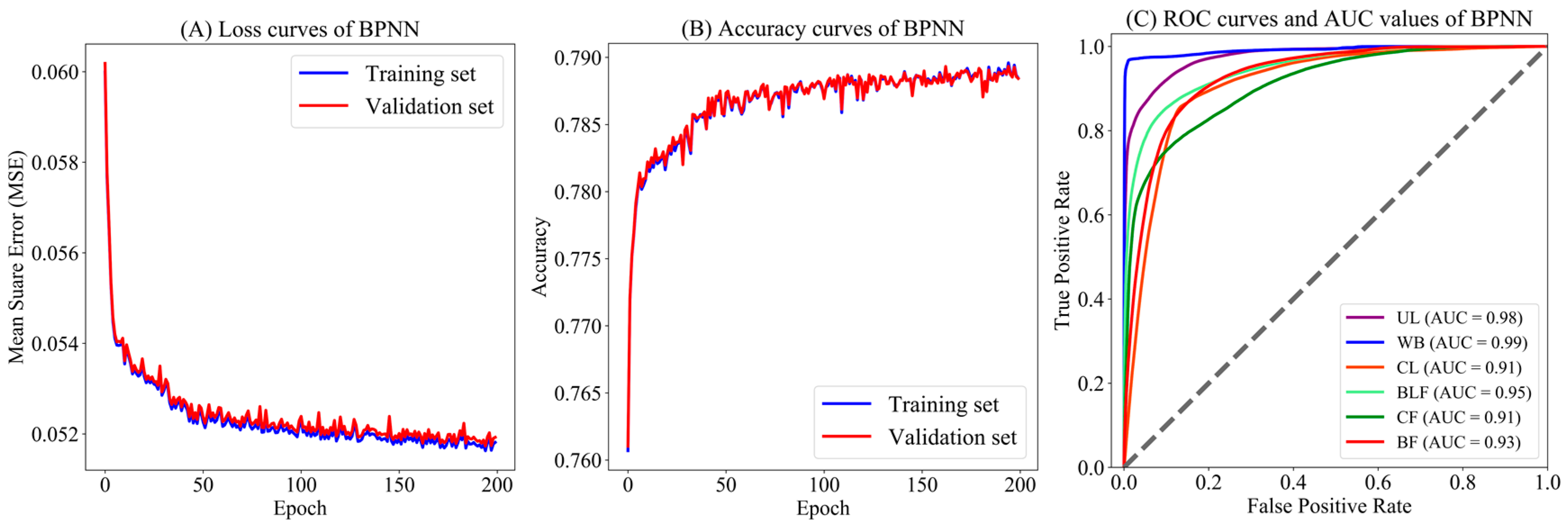
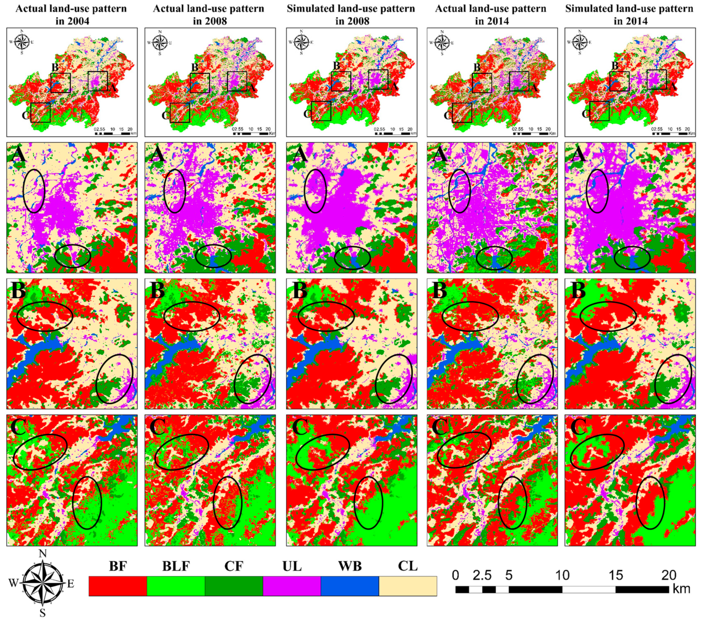
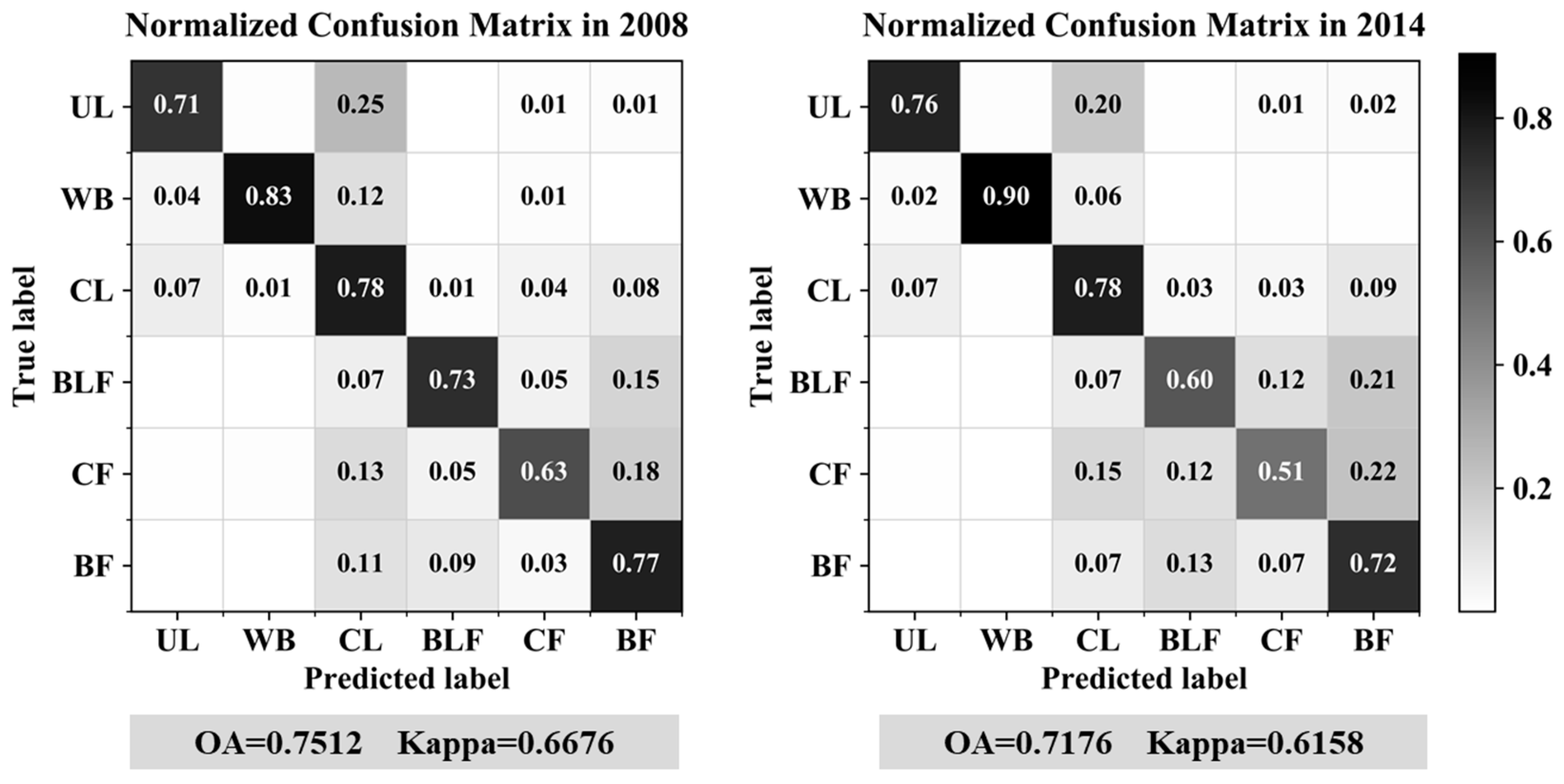
The BPNN constructed in this study has strong generalization ability and high prediction accuracy (Figure 7). Through the coupling of BPNN_CA and the Markov chain, the transformation law of LUCC in Anji County was obtained from the data for 2004, 2008, and 2014. The OAs of the two periods of simulation were above 0.7, and their kappa coefficients were above 0.6 (Figure 10), which ensured that the model provided an important solution for predicting LUCC in different climate scenarios. Meanwhile, Figure 10 shows that the longer the forecast time scale is, the lower the forecast accuracy. However, the FOM value of the simulation results in 2014 was higher than the FOM value in 2008. The main reason for this difference is that there is a relationship between FOM and the net change in actual LUCC. This relationship will cause the FOM value of a long-term simulation to be higher than that of a short-term simulation [58,59].

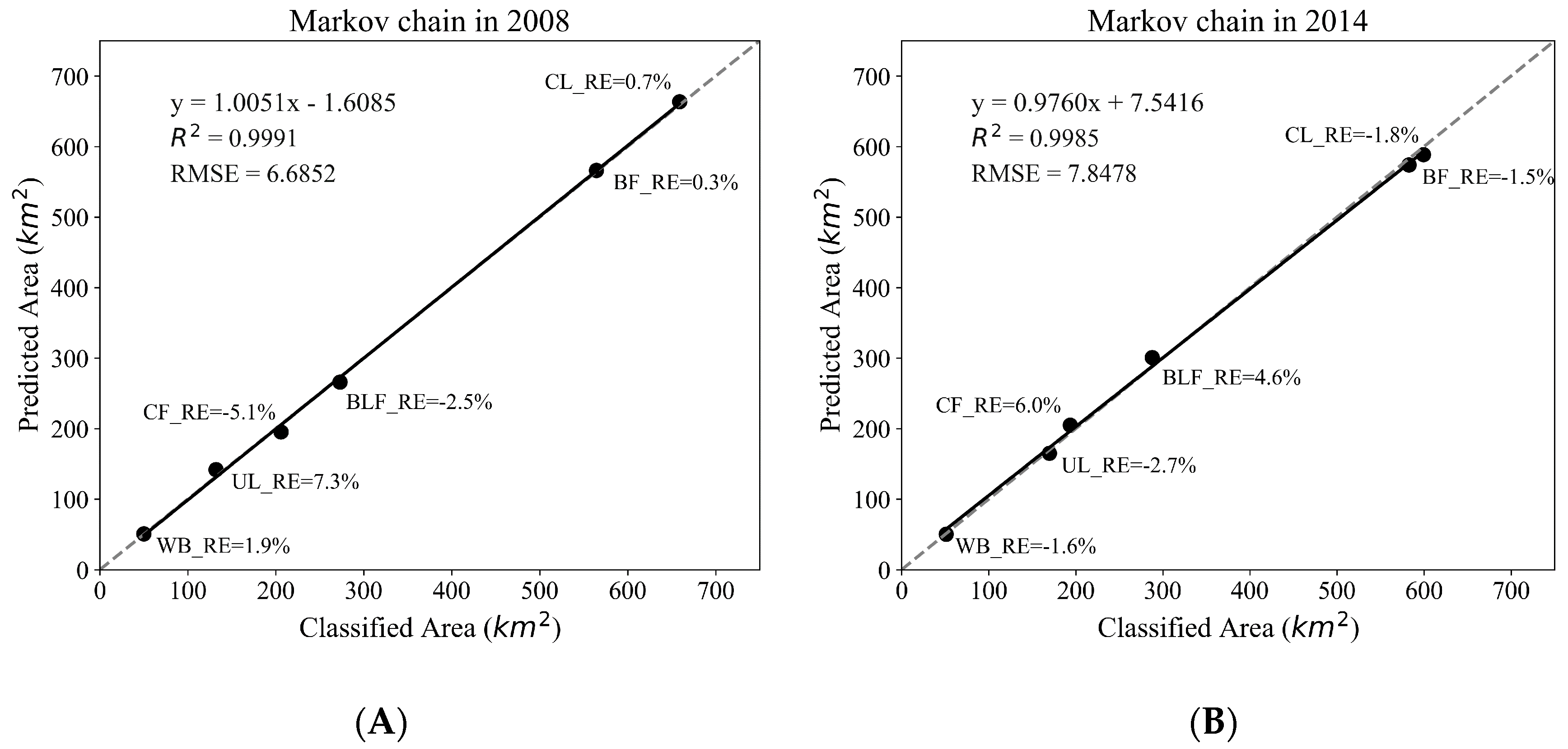
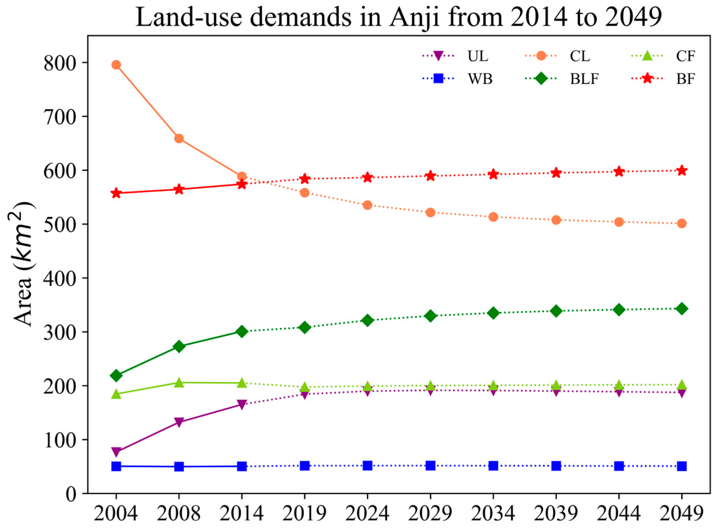
The dynamic evolution of land use has the characteristics of randomness and no after-effect [60], which conforms to the nature of the Markov chain process. Moreover, the Markov chain model can effectively combine human factors and land use and obtain future land-use demand changes based on past data [17,53]. Based on the past land-use classification, the Markov chain was used to predict the future land-use area demands of Anji County, indicating that the Markov chain can well control the land-use evolution under future weather scenarios (Figure 5 and Figure 10). The error of each land-use area is approximately 5% in the Markov chain. However, there are still some shortcomings in the Markov chain. The quantity demands under future scenarios are all set by humans according to their research needs [52,61]. For different RCP climate scenarios, the relationship between different forest tree species is not clear enough; thus, it is difficult to accurately establish the quantity requirements of different forest species. To obtain the future area of bamboo forests and other land types more accurately, it is necessary to use SD models and other methods to set different quantitative requirements relative to different climate scenarios [7,56,62].

LUCC is also the result of the comprehensive influences of complex and diverse factors. Considering a variety of driving factors, the ROC curves and AUC values of the BPNN are different in each land-use type, illustrating that the transformation of land-use types is affected by driving factors to different degrees (Figure 7C). The driving factors, such as the distances to roads and water, restrict the transformation of UL and WB. Their AUC values are 0.98 and 0.99, respectively, which are higher than those of other land-use types; thus, the transformations of UL and WB are clearer. Certainly, there are still many uncertain factors for land-use changes that have not been considered in this study. The accuracy of the BPNN model to extract the characteristics of each driving factor to obtain the LUCC law can be improved. For example, approximately 20% of UL was incorrectly predicted as CL in 2008 and 2014 (Figure 10), so we can later introduce relevant data such as the spatial distribution of population density to distinguish UL from CL. For the competition among the three forest types, factors such as the size of the timber harvest and the growth mechanism of the tree species can be considered later [5]. The expansion and succession of BFs are not only related to climate change but are also affected by human activities and their own growth conditions [38]. In future research, how to add these factors to make more accurate simulation predictions is a difficult challenge to overcome. Although the BPNN can obtain the land suitability of the environment quickly and accurately, it does not quantitatively reveal the individual contributions of the driving factors to LUCC during modeling, such as logistical regression and other methods [23]. How to interpret the neural network model is still a difficult issue in the field of computer science and needs to be explored in future work [63].

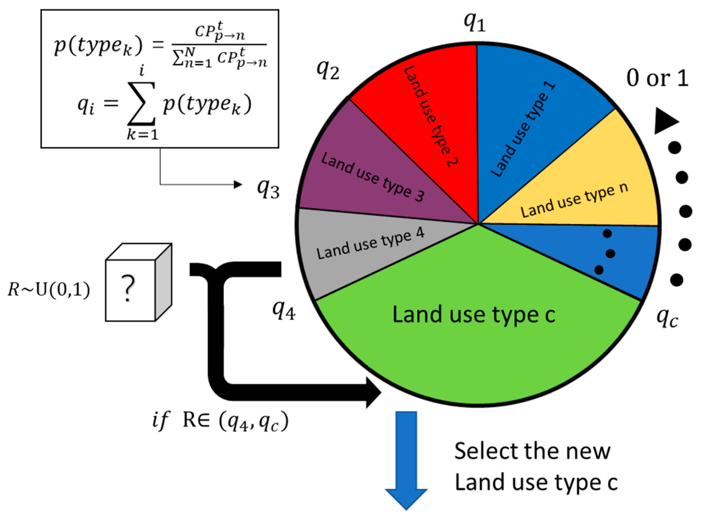
There is no unified standard for the CA model to explore the internal competition rules of LUCC. Parameters such as neighborhood weight and conversion cost are generally established by referring to expert experience and artificial optimization. In this study, the distribution method of the CA model used the roulette mechanism instead of the stochastic disturbance term. The reason is that the stochastic disturbance term will change the probability value of each pixel and change the ratio of low-probability events to high-probability events to a certain extent, which cannot show the status of the original probability [13,56], while the roulette mechanism can retain the dominant position of high-probability events [7]. The roulette mechanism has certain advantages in its allocation method, but it also introduces randomness, which leads to the difference between the simulated LUCC and the actual LUCC, which can be seen from the C and D values in Table 7.

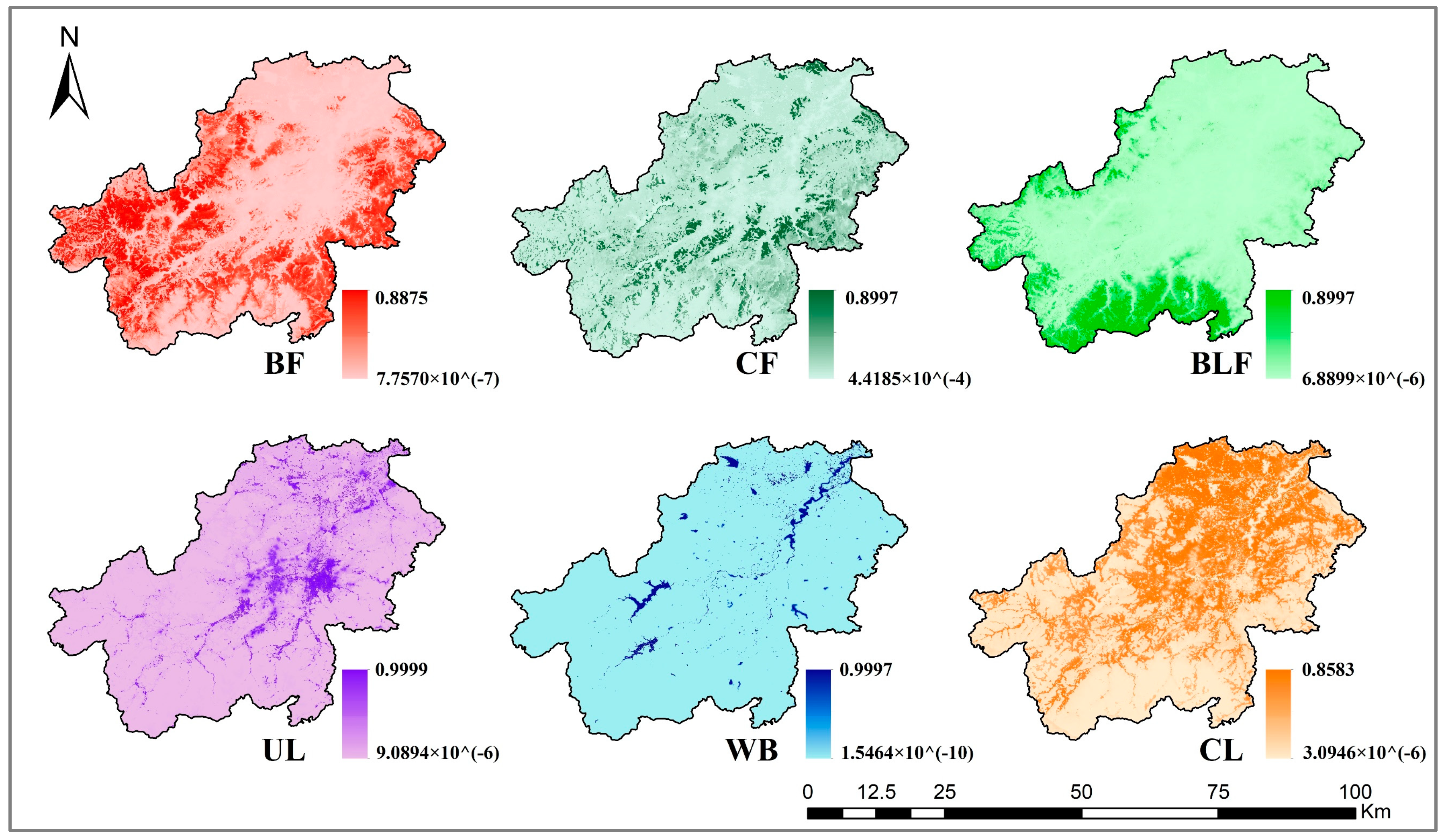
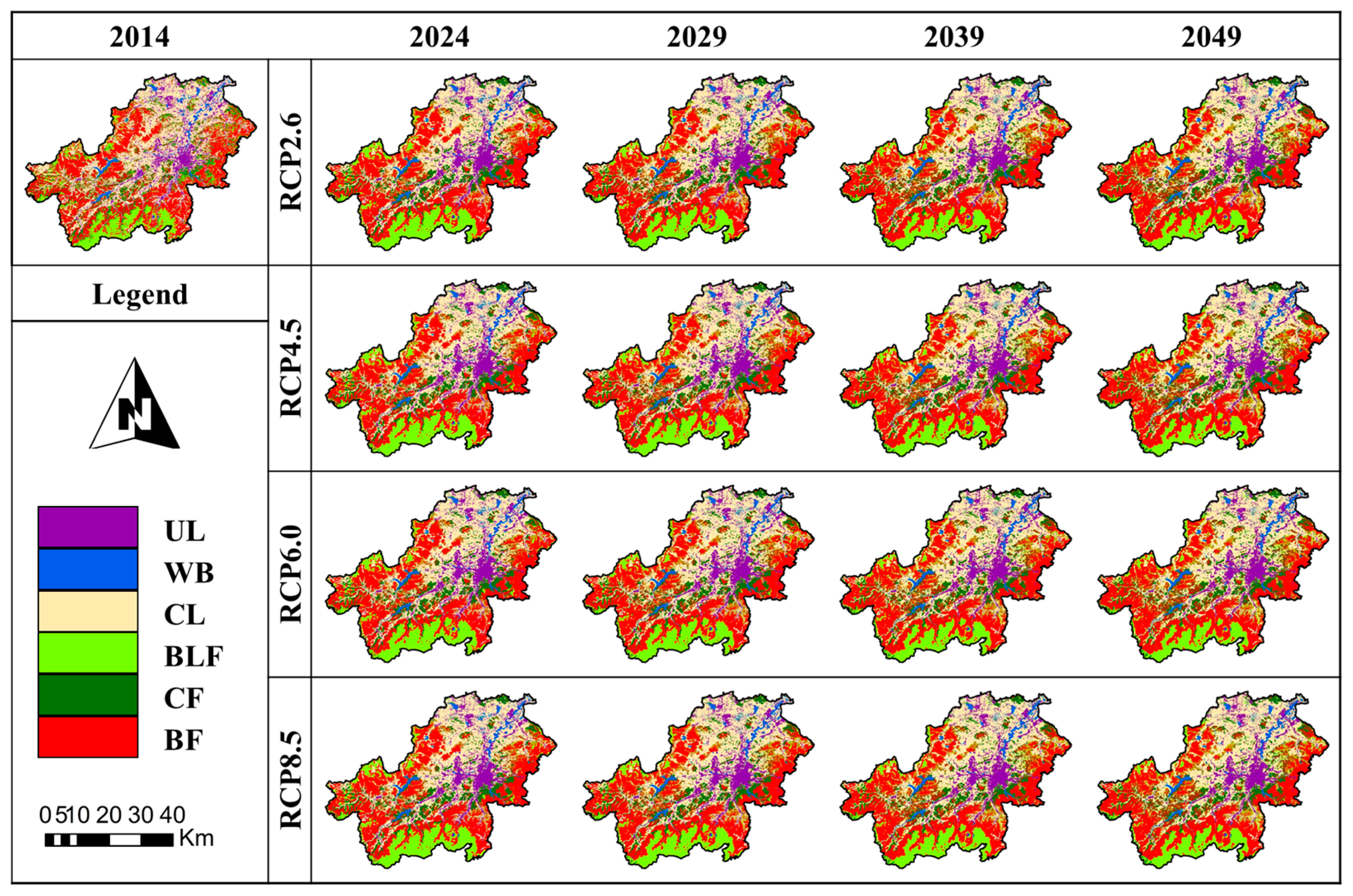
In the future spatial distribution map simulated by the BPNN_CA_Markov coupling model (Figure 12), the spatial distribution of each land-use type does not change significantly under different climate scenarios. The reason is that the use of climate data with a resolution of 1 km to drive the spatial distribution of land use with a resolution of 30 m has certain disadvantages. At the same time, the scale of the study area is small, and land-use changes are not obvious. However, this study provides a model basis for subsequent low-resolution LUCC simulations on a large scale.

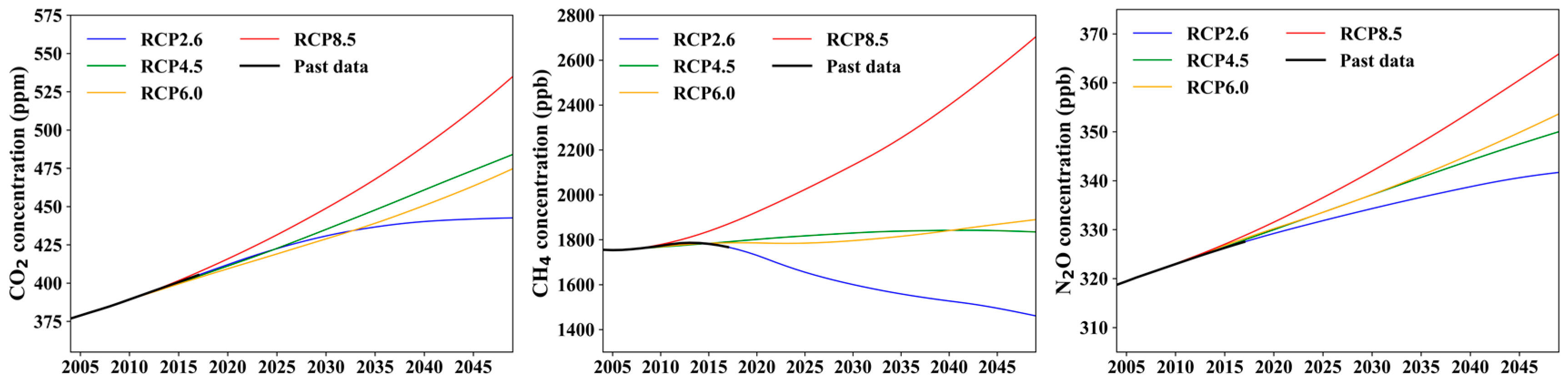
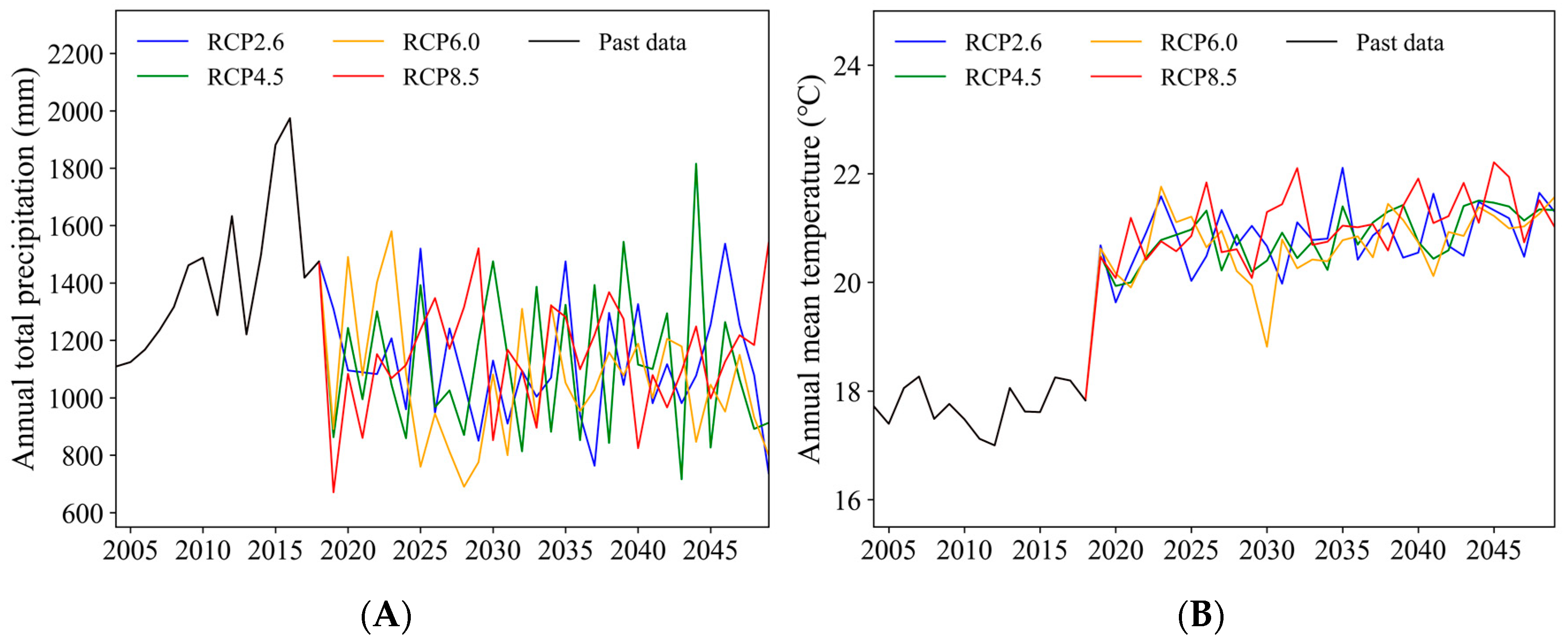
The growth of BF is affected by the climate and has certain requirements on precipitation and temperature. The annual total precipitation required for bamboo growth is 1200–2500 mm, and the average daily temperature conducive to bamboo growth is in the range of 15°–25° [64]. The annual total precipitation in Anji County will be 750–1750 mm under the four future climate scenarios, and the average daily temperature will be between 18° and 22° (Figure 15), indicating that Anji County is still suitable for bamboo forest growth in the future. Therefore, the BF area predicted by the Markov chain will expand steadily (Figure 11), which conforms to the actual situation to some extent.

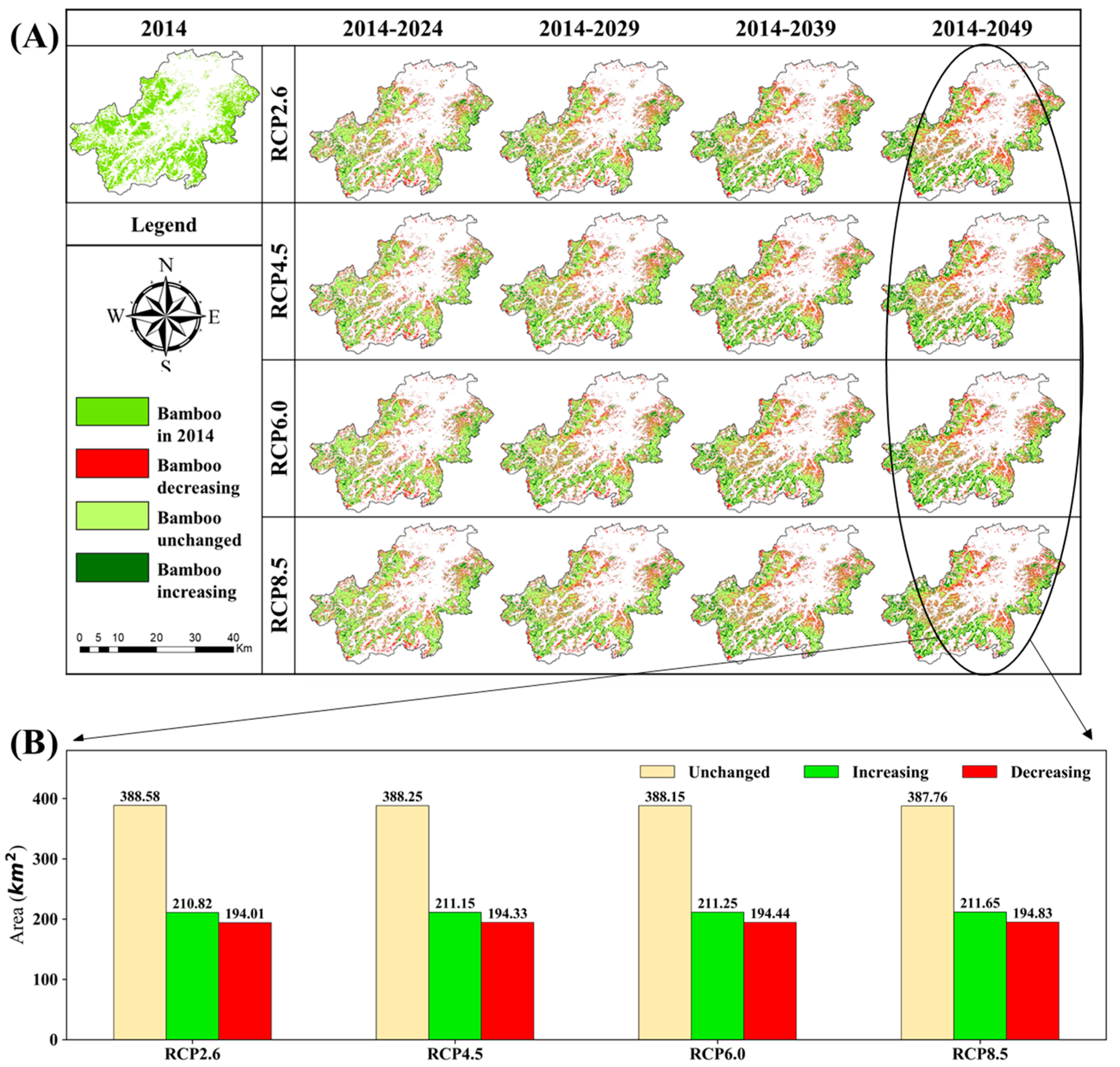
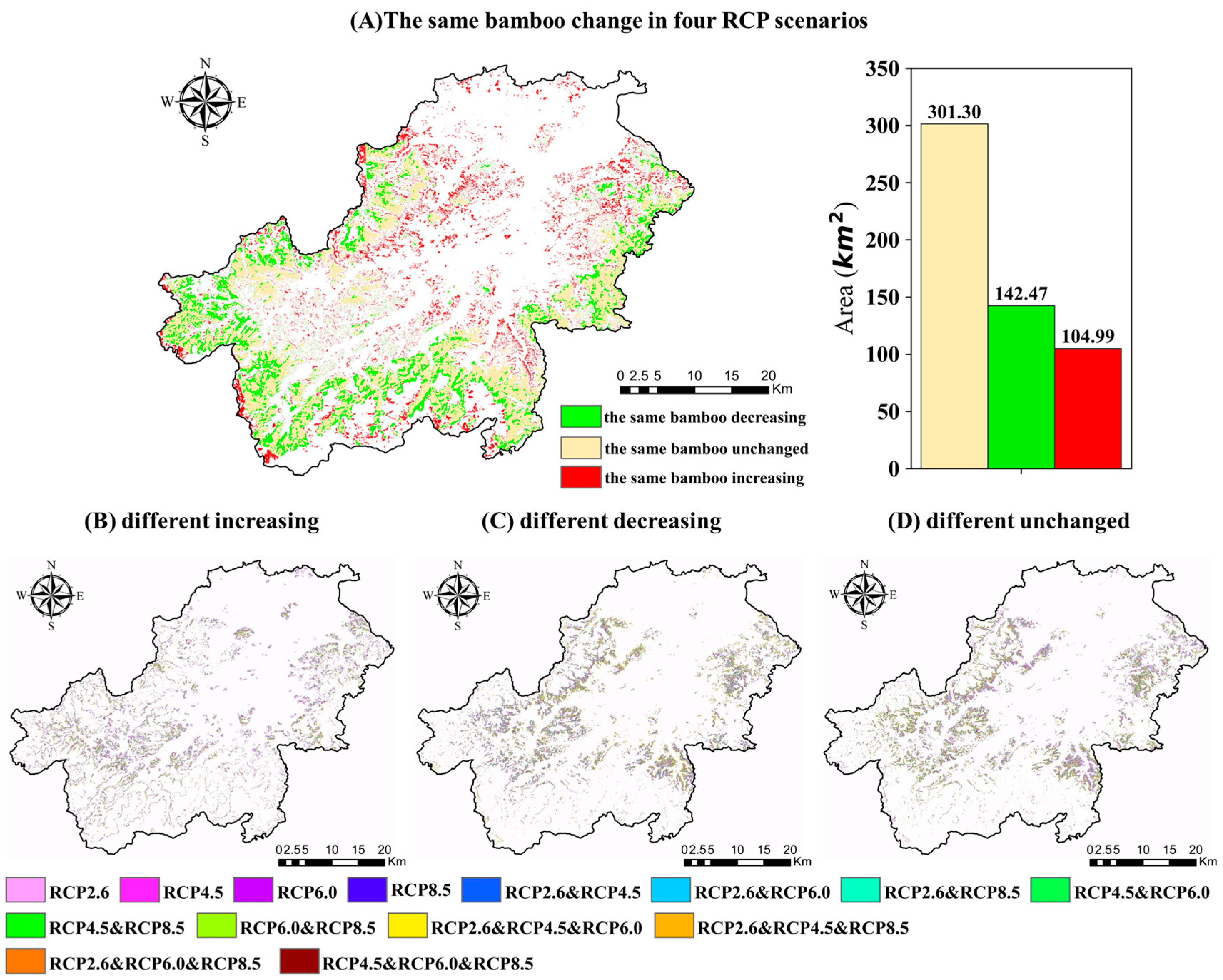
The greenhouse gas emissions, precipitation, and temperature in Anji County under the four climate scenarios differ from year to year (Figure 2 and Figure 15), resulting in differences in the BF distribution under each scenario. Figure 13 shows that there is the least damage to the BF under the RCP2.6 scenario. Compared with other scenarios, the BF changes from 2014 to 2049 are the most stable and have the smallest spatial scope in this scenario. This result is mainly because the RCP2.6 scenario is a relatively conservative development strategy scenario. Under this scenario, GDP, population growth rate, and technological innovation are at the lowest levels, and forest restoration is promoted, which is conducive to the preservation and expansion of BF. As greenhouse gas emissions increase, leading to changes in precipitation, temperature, and radiation, the environment gets worse, and the scale of bamboo forest expansion and contraction widens, and a larger area gets damaged [38]. If we simulate the BF distribution according to actual different quantity requirements relative to different climate scenarios, the area of BF at RCP8.5 will be much lower than that at RCP2.6. With reference to the RCP2.6 scenario, the government can establish corresponding climate policies to reduce the negative impact of climate change on BF for the sustainable management of bamboo forest resources.

5. Conclusions

Simulating spatiotemporal LUCC data precisely under future climate scenarios is an important basis for revealing the carbon cycle response of forest ecosystems to LUCC. In this paper, a coupling model consisting of BPNN, Markov chain, and cellular automata (CA) was designed to simulate the LUCC in Anji County, Zhejiang Province, under four climate scenarios (RCP2.6, 4.5, 6.0, 8.5) from 2024 to 2049 and to analyze the temporal and spatial distribution of bamboo forests in Anji County. The studies we performed show that (1) the transition probability matrices indicate that the area of bamboo forests shows an expansion trend, and the largest contribution to the expansion of bamboo forests is the cultivated land. The Markov chain composed of the average transition probability matrix could perform excellently with small errors when simulating the areas of different land-use types. (2) Based on the optimized BPNN, which had a strong generalization ability, a high prediction accuracy, and AUC values above 0.9, we could obtain highly reliable land-use transfer rules and land suitability probabilities. After introducing more driving factors related to bamboo forests, the prediction of bamboo forest changes will be more accurate. (3) The BPNN_CA_Markov coupling model could achieve a high-precision simulation of LUCC at different times, with an overall accuracy greater than 70%, and the consistency of the LUCC simulation from one time to another also had good performance, with an FOM of approximately 40%. (4) Under the future four RCP scenarios, bamboo forest evolution has similar spatial characteristics; that is, bamboo forests will expand in the northeast, south, and southwest mountainous areas of Anji County, while bamboo forests will decrease mainly around the junction of the central and mountainous areas of Anji County. Comparing the simulation results of different scenarios demonstrates that 74% of the spatiotemporal evolution of bamboo forests will be influenced by internal land-use competition and other driving factors, and 26% will come from different climate scenarios, among which the RCP8.5 scenario will have the greatest impact on the bamboo forest area and spatiotemporal evolution, while the RCP2.6 scenario will have the smallest impact. In short, this study proposes effective methods and ideas for LUCC simulation in the context of climate change and provides accurate data support for analyzing the impact of LUCC on the carbon cycle of bamboo forests.

References

1. Jiao, J.-G.; Yang, L.-Z.; Wu, J.-X.; Wang, H.-Q.; Li, H.-X.; Ellis, E.C. Land Use and Soil Organic Carbon in China’s Village Landscapes. Pedosphere 2010, 20, 1–14. [Google Scholar]
2. Matthews, H.D.; Graham, T.L.; Keverian, S.; Lamontagne, C.; Seto, D.; Smith, T.J. National contributions to observed global warming. Environ. Res. Lett. 2014, 9, 468–475. [Google Scholar] [CrossRef] [Green Version]
3. Su, Z.-Y.; Xiong, Y.-M.; Zhu, J.-Y.; Ye, Y.-C.; Ye, M. Soil Organic Carbon Content and Distribution in a Small Landscape of Dongguan, South China. Pedosphere 2006, 16, 10–17. [Google Scholar]
4. Law, B.E.; Hudiburg, T.W.; Berner, L.T.; Kent, J.J.; Buotte, P.C.; Harmon, M.E. Land use strategies to mitigate climate change in carbon dense temperate forests. Proc. Natl. Acad. Sci. USA 2018, 115, 201720064. [Google Scholar] [CrossRef] [Green Version]
5. Wu, Z.; Dai, E.; Wu, Z.; Lin, M. Future forest dynamics under climate change, land use change, and harvest in subtropical forests in Southern China. Landsc. Ecol. 2019, 34, 843–863. [Google Scholar] [CrossRef]
6. Yu, Z.; Lu, C.; Tian, H.; Canadell, J.G. Largely underestimated carbon emission from land use and land cover change in the conterminous United States. Glob. Chang. Biol. 2019, 25, 3741–3752. [Google Scholar] [CrossRef]
7. Liu, X.; Liang, X.; Li, X.; Xu, X.; Ou, J.; Chen, Y.; Li, S.; Wang, S.; Pei, F. A future land use simulation model (FLUS) for simulating multiple land use scenarios by coupling human and natural effects. Landsc. Urban Plan. 2017, 168, 94–116. [Google Scholar] [CrossRef]
8. Marull, J.; Pino, J.; Tello, E.; Cordobilla, M.J. Social metabolism, landscape change and land-use planning in the Barcelona Metropolitan Region. Land Use Policy 2010, 27, 497–510. [Google Scholar] [CrossRef]
9. Pijanowski, B.C.; Brown, D.G.; Shellito, B.A.; Manik, G.A. Using neural networks and GIS to forecast land use changes: A land transformation model. Comput. Environ. Urban Syst. 2002, 26, 553–575. [Google Scholar] [CrossRef]
10. Stephenne, N.; Lambin, E. A dynamic simulation model of land-use changes in Sudano-sahelian countries of Africa (SALU). Agric. Ecosyst. Environ. 2001, 85, 145–161. [Google Scholar] [CrossRef]
11. Gobin, A.; Campling, P.; Feyen, J. Logistic modelling to derive agricultural land use determinants: A case study from southeastern Nigeria. Agric. Ecosyst. Environ. 2002, 89, 213–228. [Google Scholar] [CrossRef]
12. Tian, H.; Liang, X.; Li, X.; Liu, X.; Ou, J.; Hong, Y.; He, Z. Simulating Multiple Land Use Scenarios in China during 2010–2050 Based on System Dynamic Model. Trop. Geogr. 2017, 37, 547–561. [Google Scholar]
13. Li, X.; Yeh, A.G.-O. Neural-network-based cellular automata for simulating multiple land use changes using GIS. Int. J. Geogr. Inf. Sci. 2002, 16, 323–343. [Google Scholar] [CrossRef]
14. Luo, G.; Yin, C.; Chen, X.; Xu, W.; Lu, L. Combining system dynamic model and CLUE-S model to improve land use scenario analyses at regional scale: A case study of Sangong watershed in Xinjiang, China. Ecol. Complex. 2010, 7, 198–207. [Google Scholar] [CrossRef]
15. Yang, X.; Jin, X.; Du, X.; Xiang, X.; Han, J.; Shan, W.; Fan, Y.; Zhou, Y. Multi-agent model-based historical cropland spatial pattern reconstruction for 1661–1952, Shandong Province, China. Glob. Planet. Chang. 2016, 143, 175–188. [Google Scholar] [CrossRef] [Green Version]
16. Itami, R.M. Simulating spatial dynamics: Cellular automata theory. Landsc. Urban Plan. 1994, 30, 27–47. [Google Scholar] [CrossRef]
17. Han, H.; Yang, C.; Song, J. Scenario simulation and the prediction of land use and land cover change in Beijing, China. Sustainability 2015, 7, 4260–4279. [Google Scholar] [CrossRef] [Green Version]
18. Verburg, P.H.; Schulp, C.; Witte, N.; Veldkamp, A. Downscaling of land use change scenarios to assess the dynamics of European landscapes. Agric. Ecosyst. Environ. 2006, 114, 39–56. [Google Scholar] [CrossRef]
19. Marta, L.; Michelle, R.; Erika, C.; Filippo, G.; Rosmeri, D.R.; Diego, D.S. Land Use Change over the Amazon Forest and Its Impact on the Local Climate. Water 2018, 10, 149. [Google Scholar]
20. Leemans, R.; Van Amstel, A.; Battjes, C.; Kreileman, E.; Toet, S. The land cover and carbon cycle consequences of large-scale utilizations of biomass as an energy source. Glob. Environ. Chang. 1996, 6, 335–357. [Google Scholar] [CrossRef]
21. van Meijl, H.; Van Rheenen, T.; Tabeau, A.; Eickhout, B. The impact of different policy environments on agricultural land use in Europe. Agric. Ecosyst. Environ. 2006, 114, 21–38. [Google Scholar] [CrossRef]
22. Behera, M.D.; Borate, S.N.; Panda, S.N.; Behera, P.R.; Roy, P.S. Modelling and analyzing the watershed dynamics using Cellular Automata (CA)–Markov model—A geo-information based approach. J. Earth Syst. Sci. 2012, 121, 1011–1024. [Google Scholar] [CrossRef] [Green Version]
23. Jokar Arsanjani, J.; Helbich, M.; Kainz, W.; Darvishi Boloorani, A. Integration of logistic regression, Markov chain and cellular automata models to simulate urban expansion. Int. J. Appl. Earth Obs. Geoinf. 2013, 21, 265–275. [Google Scholar] [CrossRef]
24. Guan, D.J.; Li, H.F.; Inohae, T.; Su, W.; Nagaie, T.; Hokao, K. Modeling urban land use change by the integration of cellular automaton and Markov model. Ecol. Model. 2011, 222, 3761–3772. [Google Scholar] [CrossRef]
25. Tiné, M.; Perez, L.; Molowny-Horas, R. Hybrid spatiotemporal simulation of future changes in open wetlands: A study of the Abitibi-Témiscamingue region, Québec, Canada. Int. J. Appl. Earth Obs. Geoinf. 2019, 74, 302–313. [Google Scholar] [CrossRef]
26. Zhao, M.; He, Z.; Du, J.; Chen, L.; Lin, P.; Fang, S. Assessing the effects of ecological engineering on carbon storage by linking the CA-Markov and InVEST models. Ecol. Indic. 2018, 98, 29–38. [Google Scholar] [CrossRef]
27. Wang, S.; Zhang, Z.; Wang, X. Land use change and prediction in the Baimahe Basin using GIS and CA-Markov model. IOP Conf. Ser. Earth Environ. Sci. 2014, 17, 012074. [Google Scholar] [CrossRef] [Green Version]
28. Yang, J.; Chen, F.; Xi, J.; Xie, P.; Li, C. A Multitarget Land Use Change Simulation Model Based on Cellular Automata and Its Application. Abstr. Appl. Anal. 2014, 2014, 1–11. [Google Scholar] [CrossRef] [Green Version]
29. Shooshtari, S.J.; Gholamalifard, M. Scenario-based land cover change modeling and its implications for landscape pattern analysis in the Neka Watershed, Iran. Remote Sens. Appl. Soc. Environ. 2015, 1, 1–19. [Google Scholar] [CrossRef]
30. Espiritosanto, F.D.B.; Gloor, M.; Keller, M.; Malhi, Y.; Saatchi, S.; Nelson, B.W.; Junior, R.; Pereira, C.; Lloyd, J.; Frolking, S. Size and frequency of natural forest disturbances and the Amazon forest carbon balance. Nat. Commun. 2014, 5, 3434. [Google Scholar] [CrossRef] [Green Version]
31. Seidl, R.; Thom, D.; Kautz, M.; Martin-Benito, D.; Peltoniemi, M.; Vacchiano, G.; Wild, J.; Ascoli, D.; Petr, M.; Honkaniemi, J. Forest disturbances under climate change. Nat. Clim. Chang. 2017, 7, 395–402. [Google Scholar] [CrossRef] [Green Version]
32. Houghton, R.A.; Nassikas, A.A. Negative emissions from stopping deforestation and forest degradation, globally. Glob. Chang. Biol. 2018, 24, 350–359. [Google Scholar] [CrossRef]
33. Costanza, R.; Ruth, M. Using Dynamic Modeling to Scope Environmental Problems and Build Consensus. Environ. Manag. 1998, 22, 183–195. [Google Scholar] [CrossRef]
34. Verburg, P.H.; Schot, P.P.; Dijst, M.J.; Veldkamp, A. Land use change modelling: Current practice and research priorities. Geojournal 2004, 61, 309–324. [Google Scholar] [CrossRef]
35. Kline, J.D.; Moses, A.; Lettman, G.J.; Azuma, D.L. Modeling forest and range land development in rural locations, with examples from eastern Oregon. Landsc. Urban Plan. 2007, 80, 320–332. [Google Scholar] [CrossRef]
36. Schulp, C.J.E.; Nabuurs, G.J.; Verburg, P.H. Future carbon sequestration in Europe—Effects of land use change. Agric. Ecosyst. Environ. 2008, 127, 251–264. [Google Scholar] [CrossRef]
37. Zhou, G.; Jiang, P.; Du, H.; Shi, Y. Technology for the Measurement and Enhancement Carbon Sinks in Bamboo Forest Ecosystems; Science Press: Beijing, China, 2017. [Google Scholar]
38. Li, X.; Mao, F.; Du, H.; Zhou, G.; Zhang, M. Spatiotemporal evolution and impacts of climate change on bamboo distribution in China. J. Environ. Manag. 2019, 248, 109265. [Google Scholar] [CrossRef]
39. Xu, X.; Zhou, G.; Du, H.; Partida, A. Bamboo forest change and its effect on biomass carbon stocks: A case study of Anji County, Zhejiang Province, China. J. Trop. For. Sci. 2012, 24, 426–435. [Google Scholar]
40. Ruirui, C.; Huaqiang, D.; Guomo, Z.; Xiaojun, X.; Dejin, D.; Yulong, L. Remote sensing-based dynamic monitoring of moso bamboo forest and its carbon stock change in Anji County. J. Zhejiang A F Univ. 2011, 28, 422–431. [Google Scholar]
41. Poelmans, L.; Rompaey, A.V. Complexity and performance of urban expansion models. Comput. Environ. Urban Syst. 2010, 34, 17–27. [Google Scholar] [CrossRef]
42. Dubovyk, O.; Sliuzas, R.; Flacke, J. Spatio-temporal modelling of informal settlement development in Sancaktepe district, Istanbul, Turkey. ISPRS J. Photogramm. Remote Sens. 2011, 66, 235–246. [Google Scholar] [CrossRef]
43. Li, X.; Du, H.; Mao, F.; Zhou, G.; Xing, L.; Liu, T.; Han, N.; Liu, E.; Ge, H.; Liu, Y. Mapping spatiotemporal decisions for sustainable productivity of bamboo forest land. Land Degrad. Dev. 2020, 31, 939–958. [Google Scholar] [CrossRef]
44. Zheng, J.; Mao, F.; Du, H.; Li, X.; Xing, L. Spatiotemporal Simulation of Net Ecosystem Productivity and Its Response to Climate Change in Subtropical Forests. Forests 2019, 10, 708. [Google Scholar] [CrossRef] [Green Version]
45. Pachauri, R.; Reisinger, A. Climate Change 2014: Synthesis Report. Contribution of Working Groups I, II and III to the Fifth Assessment Report of the Intergovernmental Panel on Climate Change. J. Roman. Stud. 2014, 4, 85–88. [Google Scholar]
46. Zhou, G.M.; Jiang, P.K. Density, storage and spatial distribution of carbon in Phyllostachy pubescens forest. Sci. Silvae Sin. 2004, 40, 20–24. [Google Scholar]
47. Xiao, F.; Fan, S.; Wang, S.; Xiong, C.; Zhang, C.; Liu, S.; Zhang, J. Carbon storage and spatial distribution in Phyllostachy pubescens and Cunninghamia lanceolata plantation ecosystem. Acta Phytoecol. Sin. 2007, 27, 2791–2801. [Google Scholar]
48. Zhen-Qin, L. Soil Nutrients and Carbon Stocks in Phyllostachys heterocycla cv. pubescens Ecosystems at Various Elevations in Jianou City. J. Bamboo Res. 2013, 2, 7. [Google Scholar]
49. Zhang, M.; Du, H.; Mao, F.; Zhou, G.; Li, X.; Dong, L.; Zheng, J.; Zhu, D.; Liu, H.; Huang, Z. Spatiotemporal Evolution of Urban Expansion Using Landsat Time Series Data and Assessment of Its Influences on Forests. ISPRS Int. J. Geo Inf. 2020, 9, 64. [Google Scholar] [CrossRef] [Green Version]
50. Li, Y.; Du, H.; Mao, F.; Li, X.; Cui, L.; Han, N.; Xu, X. Information Extracting and Spatiotemporal Evolution of Bamboo Forest Based on Landsat Time Series Data in Zhejiang Province. Sci. Silvae Sin. 2019, 55, 88–96. [Google Scholar]
51. Surabuddin Mondal, M.; Sharma, N.; Kappas, M.; Garg, P. Modeling of spatio-temporal dynamics of land use and land cover in a part of Brahmaputra River basin using Geoinformatic techniques. Geocarto Int. 2013, 28, 632–656. [Google Scholar] [CrossRef]
52. Sanchayeeta, A.; Jane, S. Simulating Forest Cover Changes of Bannerghatta National Park Based on a CA-Markov Model: A Remote Sensing Approach. Remote Sens. 2012, 4, 3215–3243. [Google Scholar]
53. Gidey, E.; Dikinya, O.; Sebego, R.; Segosebe, E.; Zenebe, A. Cellular automata and Markov Chain (CA_Markov) model-based predictions of future land use and land cover scenarios (2015–2033) in Raya, northern Ethiopia. Modeling Earth Syst. Environ. 2017, 3, 1245–1262. [Google Scholar] [CrossRef]
54. Akin, A.; Aliffi, S.; Sunar, F. Spatio-temporal urban change analysis and the ecological threats concerning the third bridge in Istanbul City. Int. Arch. Photogramm. Remote Sens. Spat. Inf. Sci. 2014, 40, 9. [Google Scholar] [CrossRef] [Green Version]
55. He, C.; Shi, P.; Chen, J.; Li, X.; Pan, Y.; Li, Y.; Li, J. Developing land use scenario dynamics model by the integration of system dynamics model and cellular automata model. Sci. China Ser. D Earth Sci. 2005, 48, 1979. [Google Scholar] [CrossRef]
56. Huang, Q.X.; Chunyang, H.E.; Liu, Z.F.; Shi, P.J. Modeling the impacts of drying trend scenarios on land systems in northern China using an integrated SD and CA model. Sci. China Earth Sci. 2014, 57, 839–854. [Google Scholar] [CrossRef]
57. Verburg, P.H.; Soepboer, W.; Veldkamp, A.; Limpiada, R.; Espaldon, V.; Mastura, S.S. Modeling the spatial dynamics of regional land use: The CLUE-S model. Environ. Manag. 2002, 30, 391–405. [Google Scholar] [CrossRef]
58. Pontius, R.G.; Boersma, W.; Castella, J.; Clarke, K.C.; De Nijs, T.; Dietzel, C.; Duan, Z.; Fotsing, E.; Goldstein, N.; Kok, K. Comparing the input, output, and validation maps for several models of land change. Ann. Reg. Sci. 2008, 42, 11–37. [Google Scholar] [CrossRef] [Green Version]
59. Estoque, R.C.; Murayama, Y. Examining the potential impact of land use/cover changes on the ecosystem services of Baguio city, the Philippines: A scenario-based analysis. Appl. Geogr. 2012, 35, 316–326. [Google Scholar] [CrossRef]
60. Iacono, M.; Levinson, D.; El-Geneidy, A.; Wasfi, R. A Markov chain model of land use change. TeMA J. Land Use Mobil. Environ. 2015, 8, 263–276. [Google Scholar]
61. Li, K.; Feng, M.; Biswas, A.; Su, H.; Niu, Y.; Cao, J. Driving Factors and Future Prediction of Land Use and Cover Change Based on Satellite Remote Sensing Data by the LCM Model: A Case Study from Gansu Province, China. Sensors 2020, 20, 2757. [Google Scholar] [CrossRef]
62. Liao, W.; Liu, X.; Xu, X.; Chen, G.; Li, X. Projections of land use changes under the plant functional type classification in different SSP-RCP scenarios in China. Sci. Bull. 2020, 65, 1935–1947. [Google Scholar] [CrossRef]
63. Zhai, Y.; Yao, Y.; Guan, Q.; Liang, X.; Li, X.; Pan, Y.; Yue, H.; Yuan, Z.; Zhou, J. Simulating urban land use change by integrating a convolutional neural network with vector-based cellular automata. Int. J. Geogr. Inf. Sci. 2020, 34, 1475–1499. [Google Scholar] [CrossRef]
64. Zhang, Y. A study of the effects of climatic fluctuation on Chinese fir and bamboo ecological envrionment in subtropical regions of China. Q. J. Appl. Meteorl. 1995, 6, 75–82. [Google Scholar]
Figure 1. Location and natural environment of the study area: (A) land-use types in 2014, (B) elevation in 2014, (C) soil clay fraction in 2008, (D) total precipitation in 2014, (E) average temperature in 2014, and (F) average radiation in 2014.
Ijgi 09 00718 g001
Figure 2. The concentrations of greenhouse gas under different climate scenarios from 2004 to 2049.
Ijgi 09 00718 g002
Figure 3. The structure of the back propagation neural network (BPNN).
Ijgi 09 00718 g003
Figure 4. The roulette selection mechanism.
Ijgi 09 00718 g004
Figure 5. Flow chart for the simulation.
Ijgi 09 00718 g005
Figure 6. The error of Markov chain (A) in 2008 and (B) in 2014. (RE is the relative error between the simulated area of each land use and the actual classification area).
Ijgi 09 00718 g006
Figure 7. (A) The mean square error (MSE) of BPNN, (B) the accuracy of BPNN, and (C) the receiver operating characteristic (ROC) curves and area under ROC curve (AUC) values of BPNN.
Ijgi 09 00718 g007
Figure 8. The land suitability probabilities of the six land-use types in 2008.
Ijgi 09 00718 g008
Figure 9. The simulated spatial pattern of land cover from 2004 to 2014.
Ijgi 09 00718 g009
Figure 10. Normalized confusion matrices between predicted results and true label in 2008 and 2014.
Ijgi 09 00718 g010
Figure 11. Area demands of each land-use type in Anji County from 2004 to 2049.
Ijgi 09 00718 g011
Figure 12. Simulated result of Anji County in 2014 and different simulated results of Anji County in four scenarios from 2024–2049.
Ijgi 09 00718 g012
Figure 13. (A) Different simulated results of bamboo forest change in four scenarios in different periods. (B) the statistical area of the bamboo forest change from 2014 to 2049.
Ijgi 09 00718 g013
Figure 14. (A) the same regions where bamboo forests will change under the four RCP scenarios from 2014 to 2049. (B) the different regions where bamboo forests will increase under the four RCP scenarios from 2014 to 2049. (C) the different regions where bamboo forests will decrease under the four RCP scenarios from 2014 to 2049. (D) the different regions where bamboo forests will be unchanged under the four RCP scenarios from 2014 to 2049.
Ijgi 09 00718 g014
Figure 15. The annual total precipitation (A) and annual mean temperature (B) of Anji County under different climate scenarios from 2004 to 2049.
Ijgi 09 00718 g015