A Multiresolution Vector Data Compression Algorithm Based on Space Division

1
MOE Lab of 3D Spatial Data Acquisition and Application, Capital Normal University, Beijing 100048, China
2
College of Resource Environment and Tourism, Capital Normal University, Beijing 100048, China
*
Author to whom correspondence should be addressed.
ISPRS Int. J. Geo-Inf. 2020, 9(12), 721; https://0-doi-org.brum.beds.ac.uk/10.3390/ijgi9120721
Submission received: 1 October 2020
/
Revised: 26 November 2020
/
Accepted: 30 November 2020
/
Published: 2 December 2020
Abstract
:Vector data compression can significantly improve efficiency of geospatial data management, visualization and data transmission over internet. Existing compression methods are either based on information theory for lossless compression mainly or based on map generalization methods for lossy compression. Coordinate values of vector spatial data are mostly represented using floating-point type in which data redundancy is small and compression ratio using lossy algorithms is generally better than that of lossless compression algorithms. The purpose of paper is to implement a new algorithm for efficient compression of vector data. The algorithm, named space division based compression (SDC), employs the basic idea of linear Morton and Geohash encoding to convert floating-point type values to strings of binary chain with flexible accuracy level. Morton encoding performs multiresolution regular spatial division to geographic space. Each level of regular grid splits space horizontally and vertically. Row and column numbers in binary forms are bit interleaved to generate one integer representing the location of each grid cell. The integer values of adjacent grid cells are proximal to each other on one dimension. The algorithm can set the number of divisions according to accuracy requirements. Higher accuracy can be achieved with more levels of divisions. In this way, multiresolution vector data compression can be achieved accordingly. The compression efficiency is further improved by grid filtering and binary offset for linear and point geometries. The vector spatial data compression takes visual lossless distance on screen display as accuracy requirement. Experiments and comparisons with available algorithms show that this algorithm produces a higher data rate saving and is more adaptable to different application scenarios.
1. Introduction
Spatial data acquisition efficiency and accuracy have been drastically improved due to fast development of positioning technologies including global navigation satellite systems (GNSS), Bluetooth, Wi-Fi and others equipped on portable mobile devices [1,2]. Volume of big geospatial data in vector model such as trajectory of moving agents and geotagged social media posts grows exponentially and brings more challenges to efficient spatial data management, network transmission and visualization [3,4,5]. Compression of vector spatial data can relieve the pressure of these application scenarios.
In terms of the fidelity of results to original data, there are two types of vector spatial data compression methods: lossy compression and lossless compression. Lossy compression reduces the volume of data at the cost of certain data accuracy, and relevant methodologies can be roughly grouped into those based on map generalization algorithms and those based on high precision to low precision data type conversion (normally floating-point values to integer values based on rounding operation). Douglas–Peucker algorithm and relevant modified versions [6,7,8,9], Visvalingam algorithm [10,11] and natural principles-based algorithms [12,13,14] are typical ones for line simplification in map generalization by removing nodes to reduce data storage. This kind of algorithm usually simplifies the geometric details of geographical objects and reduces the number of points representing boundaries of vector objects. Map generalization can also be implemented based on spatial to time-frequency domain transformations, such as discrete wavelet transformation (DWT) and discrete cosine transformation (DCT) [15,16,17] by converting spatial domain information to frequency domain information and filtering high frequency coefficients after quantization. This type of algorithm is normally used in raster data and image compression, for example JPEG 2000 [18]. Another type of transformation can be implemented based on data type transformation which normally truncate coordinate values in double precision floating-point type to values in single precision floating-point type values or integers [19,20]. Vector data tiling can be applied to reduce data extent to enable value converting to an even smaller byte integer, with which a data rate saving of 80% can be achieved [20]. Lossless compression algorithms are mainly based on information theory, such as Huffman encoding, LZ series encoding [21,22], which are based on data redundancy evaluation and dictionary building. This kind of algorithm can achieve error-free decoding and is mostly used for file compression and data archiving, which can be applied in data compression of vector file or internet transmission. Another type of lossless vector data compression can be implemented based on specific properties of geometric structures. Isenburg, etc. implemented an algorithm based on parallelogram predictor of floating-point values of vertices of neighboring triangles over a surface mesh and compress the difference between predicted and actual sign, exponent, and mantissa separately using context-based arithmetic coding [23]. Although the data rate saving of this algorithm is not significant considering volume of big geospatial data generated by growing mobile agents [2], it offers an idea on how to take advantage of the geometric characteristics of vector spatial objects.
Vector data normally uses floating-point values which represents a greater range of values comparing integer values, especially when a global geospatial database shall be managed. In most application scenarios, a geospatial database can be divided regularly to smaller tiles accordingly to a predefined grid, for example using topographic sheets’ boundaries. In this way, the extent of each tile is much smaller and can be represented with an integer values with an appropriate conversion and value scaling, which can meet requirements for many applications, especially for screen visualization. With integer values, information redundancy increases, which generates possibility of data compression. During data type conversion, error estimation of data compression is vital to maintain accuracy of vector geospatial data. The conversion can be implemented in a direct float value truncation to integer [20]. It can also be implemented by regular space division. To achieve a consistent space division, a common strategy is to conduct division in global geographic space. Equilateral triangle, square and regular hexagon are three basic division geometric structures for a regular global discrete grid [24,25]. S2, H3 and Geohash encoding schema received research attention and they are used in web map applications and spatial indices. S2 encoding is based on spherical geometry that can be extended to Hilbert space filling curve [26]. H3 encoding is based on a regular icosahedral multiresolution hexagonal grid [27]. Geohash encoding is based on vertical and horizontal cross division [28,29]. Morton encoding and Geohash encoding basically follow similar ideas to encode a geographic range (normally a rectangle) into a string or an integer value [28]. Geohash encoding is designed for global spatial divisions. It transforms two-dimensional adjacent grid cells into one dimensional linear adjacent numbers or strings with same prefix. The Geohash code length or Morton code value range of encoding results depends on the level of spatial division which can be different at various parts of research area and adaptive to local complexity of spatial objects. This property has been applied in geospatial data indexing [30] and point cloud data compression [31]. It is particularly useful for raster data compression since the origin of 2D space for encoding is upper left which meets the requirement of raster data management [32]. The characteristics of variable length at different resolution can be used for multiscale expression of vector object targets under different geometric accuracy requirements [33].
This paper designs and implements a hybrid encoding algorithm based on Morton and Geohash encoding for the purpose of efficient vector spatial data compression. The algorithm takes into account the extent of the study area, transforms the coordinate value into integer binary coding and reduces the coding length. At the same time, since point features can be sorted spatially and boundary points of geospatial features are always adjacent to their preceding and succeeding points, regular space division normally allocate them into nearby grid cells. Furthermore, points located in one cell can be filtered and a point may be referenced to its preceding point. After this introduction, the implementation method including the encoding strategy together with the idea of grid filter and offset storage is explained. Then experimental results are presented with four test datasets. The third section compares this paper’s algorithm with lossless compression and a data type conversion algorithm. Finally, future works are discussed.
2. Methodology
2.1. A Hybrid Implementation of Morton Encoding and Geohash Encoding
Space division based compression (SDC) incorporates ideas of Morton encoding and Geohash encoding. Morton encoding divides a two-dimensional geographic space into regular grids and each cell’s position represented by row and column is converted to one integer value resulted by bit interleaving operation of row and column numbers [34]. An advantage of Morton encoding is that neighboring grid cells in the two-dimension (2D) space is mapped into a one dimension (1D) linear sequencing order and keep the 2D neighboring relationship in 1D at variable resolutions. This encoding scheme is mostly used in quad-tree data model for spatial data indexing and raster data compression [32]. Geohash encoding follows a similar idea with Morton encoding. A unique property of Geohash encoding is that the encoded results at different resolutions share the same prefix. The implementation of Geohash encoding is conducted through an alternate spatial division vertically and horizontally. To implement a hierarchical space division and maintain advantages of both encoding strategies, a hybrid algorithm is designed and the basic idea can be demonstrated using an example below.
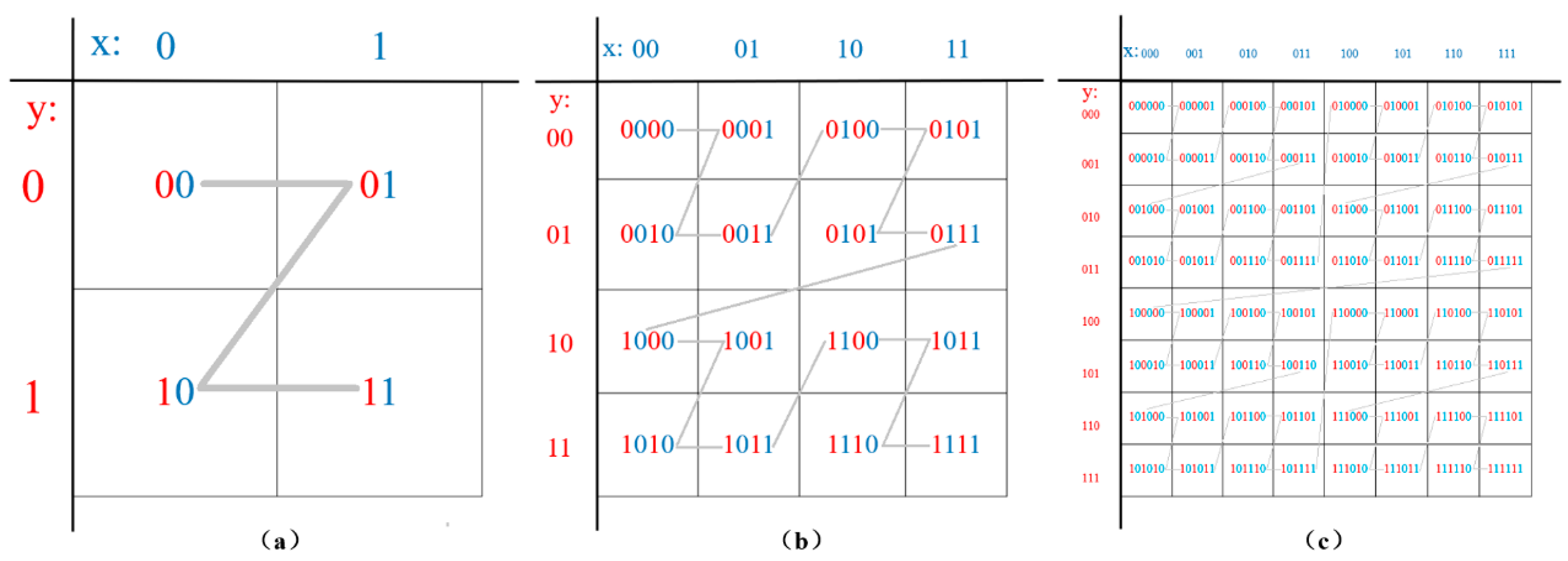
Supposing the study area of (114° E to 120° E, 40° N to 44° N) is going to be encoded. First, the central value in latitude direction, 42°N, is used to divide the area into two horizontal regions. The subregion greater than 42° N (the upper rectangle) is marked as 1, and that smaller than 42° N (lower rectangle) is marked as 0. Then the central value in longitude direction, 117° E, is used to divide the region vertically. The subregions greater than 117° E are marked as 1 and each corresponding cell’s code is appended with a character “1”. The subregions smaller than 117° E are marked as 0 and each corresponding cell’s code is appended with a character “0”. The generated binary code is alternately stored as “00”, “01”, “10”, “11”, which corresponds to the numbers of the first-level spatial division grid. The space can be further divided into finer resolution grid following the same space division strategy until the resolution meets the accuracy requirement of applications or a predefined level, as shown in Figure 1.
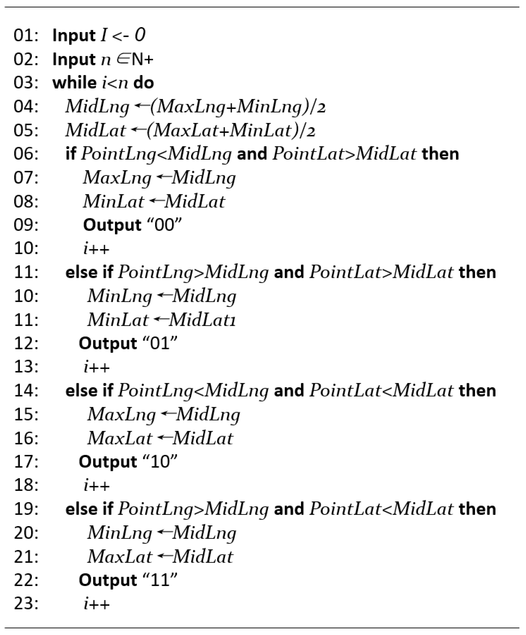
Multiresolution spatial division can be achieved by controlling levels of divisions. Encoding process of a higher resolution grid can be expanded based on its corresponding lower resolution grid encoding results. With more levels of space divisions, the grid resolution is getting finer and a longer binary code is generated, which further results in more accurate coordinates. We suppose a specific point with coordinate as (117.67198438° E, 42.1855639° N). The compression locates the grid cell containing this point and then corresponding Morton code in form of integer is used to substitute original floating-point coordinates. A pseudocode snippet is presented in Figure 2 showing the process of encoding.
In Figure 2, MinLat and MinLat are the minimum and maximum latitude values of the given research region. PointLat and PointLng are the latitude and longitude of the given point. MinLng and MaxLng are the minimum and maximum longitude values of the research region. Furthermore, variable n is the recursion time.
In grid levels with different resolutions, coordinate values stored in the form of floating-point are converted into binary codes of different length, as shown in the Table 1 with examples of binary codes. With more recursion times, a longer binary code is generated corresponding to a high precision representation. Compared with available methods of mapping geographic space to a fixed integer or short integer space, this method is more adaptive to multiscale encoding.
2.2. Grid Filter
Under a certain resolution, multiple coordinate points may fall in one grid cell, and they have one identical binary code. For multiple nodes of one vector object, a grid filtering process is conducted to replace multiple coordinate points in a grid cell with the geometric center point of this cell, as shown in Figure 3.
This operation reduces accuracy and may incur inconsistencies. So, it is an optional process and compression efficiency introduced by grid filtering is related to grid resolution. As grid resolution gradually increases, number of points in one grid cell decreases and grid filter ratio becomes lower. Grid filtering process reduces the number of coordinate points and further improves data rate saving.
2.3. Binary Offset Storage
With hybrid encoding strategy, resulted codes share same prefix in one specific area at different resolutions and present an advantage that proximity in two-dimensional space is maintained on one-dimensional space filling curves. For a given spatial object, points comprising its boundary are normally near to each other. So, encoded results of consecutive points share identical or similar binary encoded values. Then their position deviations can be recorded in resulted value of bit offset as well, which can further reduce storage volume. The offset bits length increases as the starting point bit length increases, which further depends on the grid resolution. When geographic features are more clustered, this process can be more effective.
For point features, each point is an independent vector object. After sorting according to their binary code, offset of neighboring points can be reduced and offset of each point from its preceding point can be record. Steps are as follows:
- (1)
- Sort points according to their corresponding binary codes.
- (2)
- Take the first point as origin, and all following points are presented in binary form using the number of grid cells (steps in the Morton order) that deviates from its preceding point.
- (3)
- Length of offset binary code will be greater than 1 and less than the length of the original binary code, and the maximum length of all offset binary code lengths will be taken as the storage length.
- (4)
- For records with insufficient offset bits, supplementary bits are added and filled with “0” to ensure uniform storage length.
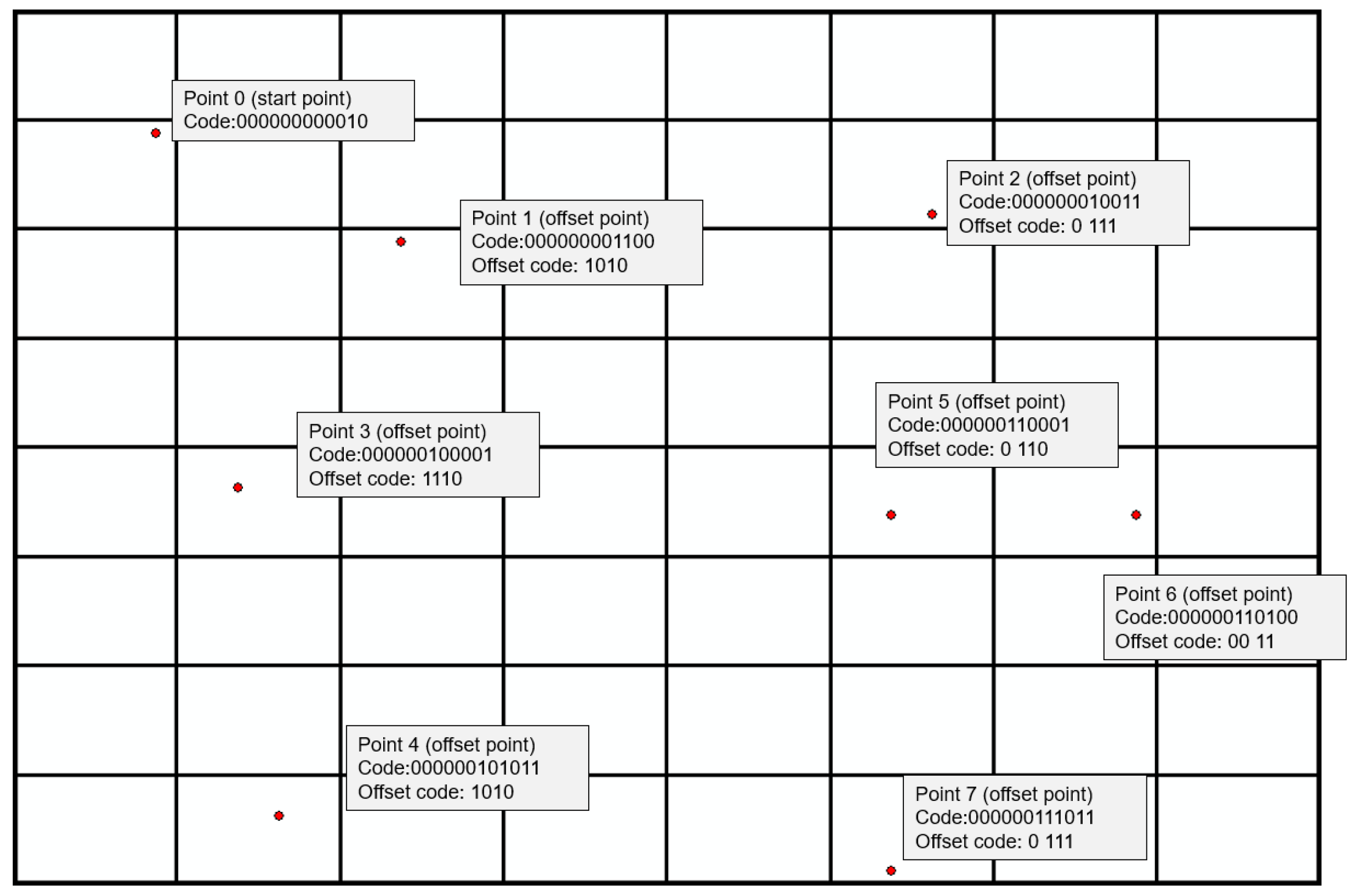
Figure 4 shows the offset storage of point features, and the grid divisions number is 6 in this figure.
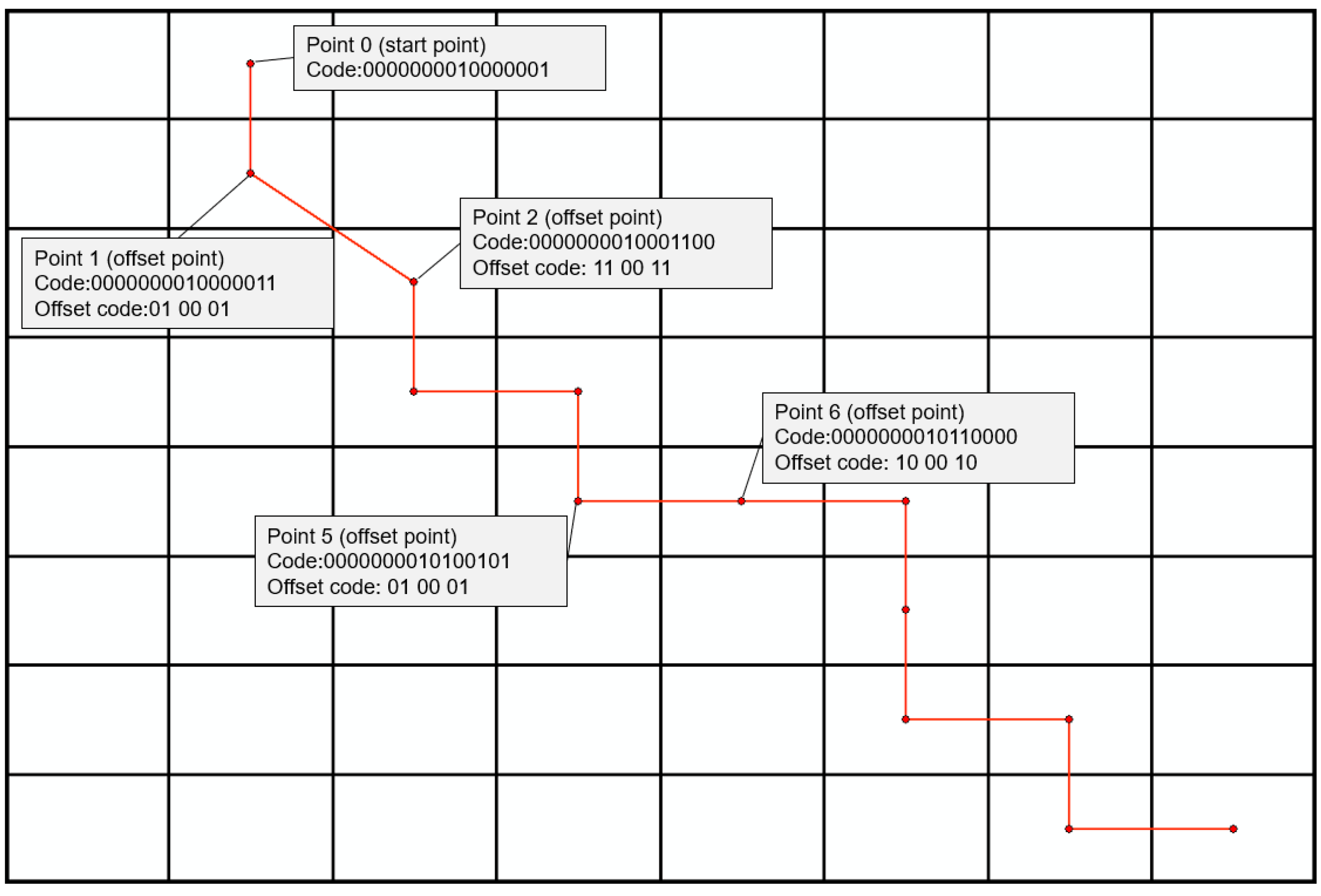
For linear or polygon features, points comprising their boundaries are managed in an ordered sequence. So, the number of points and the direction of offset of each point relative to its preceding point should be maintained. Steps are as follows:
- (1)
- Record the number of nodes and starting point coordinates of each vector object, then calculate offset in the unit of the vector object.
- (2)
- Set up direction bit, calculate the offset direction of each coordinate point to its preceding point, Use “0” or “1” to represent left or right in horizontal direction, downward or upward in vertical direction, respectively.
- (3)
- Calculate offset, record offsets of rows and columns along latitude and longitude directions, convert them into binary codes and store them alternately as the final offset.
- (4)
- Determine offset binary code length as the maximum length of all offset binary code lengths.
- (5)
- For records with insufficient offset bits, set up supplementary bits, fill with “0” to ensure uniform storage length.
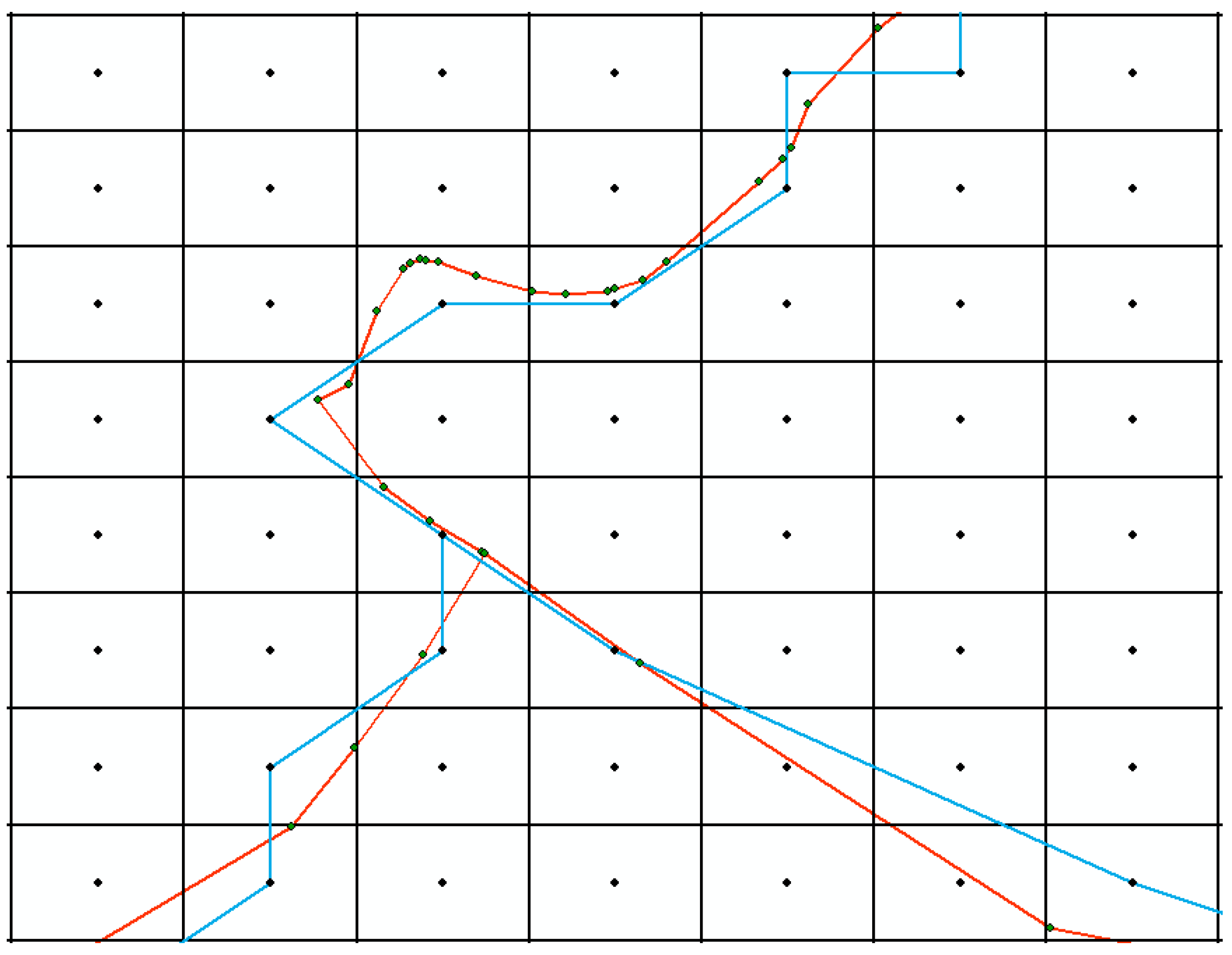
Figure 5 shows the offset storage of line or polygon features, and the grid divisions number is 8 in this figure.
2.4. Error Evaluation
Data rate saving ratio depends on levels of space division. Fewer space division levels induce lower grid resolution and greater accuracy losses. On another side, when there are more space divisions, information redundancy is suppressed and further data rate saving is getting lower. How to determine an appropriate number of space division, or grid resolution, to achieve a balance of data accuracy and data-rate saving is a key question here. This paper employs visual lossless as a controlling parameter for purposes of vector data visualization. If compressed data meets the requirement of displaying indiscernible from original data, it can be understood that accuracy is maintained for visualization purposes.
Considering capability of human eyes, 0.4 mm on paper map is the minimum required to ensure visual discernibility [35]. From the perspective of computer screen resolution, for a 100 dpi display screen, there are 100 pixels in one inch on the screen, and one pixel represents 0.01 inches, which is about 0.025 mm. So, a distance of 0.025 mm can be taken as the minimum distance (min_res_dis) to display vector information, and the ground distance (Min_Res_Dis) is:
where Scaled is map scale’s denominator, and Ratio is map magnification ratio on screen of original vector data.
In data compression process, the center point of a regular grid cell is used to replace points in the corresponding grid cell, which causes position deviation. For a regular rectangular grid, the maximum error from the point in the grid to the center point is half of the diagonal of the grid cell size. Therefore, calculation formula for defining the maximum division error (Max_Error) is
where width and height are the width and height of the research region, and n is the number of space divisions.
When Max_Error < Min_Res_Dis, visual lossless compression can be achieved. For a research region of 114° E to 120° E and 40° N to 44° N at a scale of 1:1,000,000, the evaluation table of division accuracy is shown in Table 4:
When the number of divisions is 11, the map can be displayed visual lossless without magnification. When the number of divisions is 16, the binary code length is exactly the storage size of the short integer, and the visual lossless display can be achieved when the map is enlarged by 36 times. Using more division times can meet the requirement of higher magnification display.
3. Data and Experiment Results
Four datasets were used to test the performance of space division-based compression. The first two datasets are polylines of road layer (LRDL.shp, Figure S1) and points of resident villages (RESP.shp, Figure S2) from a 1:1,000,000 topographic map. These data range between 114° E and 120° E and 40° N and 44° N. The data size of LRDL.shp is about 4075 KB and that of RESP.shp is about 44 KB. The third and fourth datasets are from OpenStreetMap [36]. The third is a natural point layer (gis_osm_natural_free_1.shp, Figure S3) covering majority region of Spain, which is about 16,129 KB. The fourth is a road layer (gis_osm_roads_free_1.shp, Figure S4) covering territory of Albania, which is about 347 MB. All the data is in Esri shapefiles format and the abovementioned sizes refer to the corresponding shapefiles (without consideration all attribute files and index files).
3.1. Visual Comparison
To the first two datasets, the compression results with different space division levels are displayed in Figure 6.
When the level of space division is 8 and 9, there are visual distortions in the compression results, which do not meet the requirement of visual lossless. When the number of divisions reaches 10, the compression result that can meet the visualization requirement at 1:1,000,000 as display scale can reach 97.18%. However, visual errors are obvious when the map is zoomed in, as shown in Figure 7, where the compressed result is overlaid with the original vector data
Figure 8 shows overlaid results of original vector data and compressed results when the level of divisions is 15. When display scale is 1:25,000, the deviation also can be maintained as visual lossless.
3.2. Data Rate Saving and Comparison
In the vector data compression process, points stored in floating-point data are converted to binary code generated by space division. Then, grid filtering reduces the number of coordinate points. Furthermore, binary offset processing further improves storage efficiency. Finally, the vector data rate saving of the test datasets under different division times is shown in Table 5. The size in each row of the “Compressed file size” column here refers to the total size of a corresponding geometry file and an object index file resulted from dumping compressed contents in memory to disks.
The four datasets were compressed using LZMA [37] algorithm with 7-zip, a free and open source file compression tool and using LZX [38] algorithm with makecab.exe, a Microsoft Windows native compression tool. Table 6 shows the compression results with these two lossless compression tools. Compared with these file compression algorithms, the method in this paper has a high data compression saving.
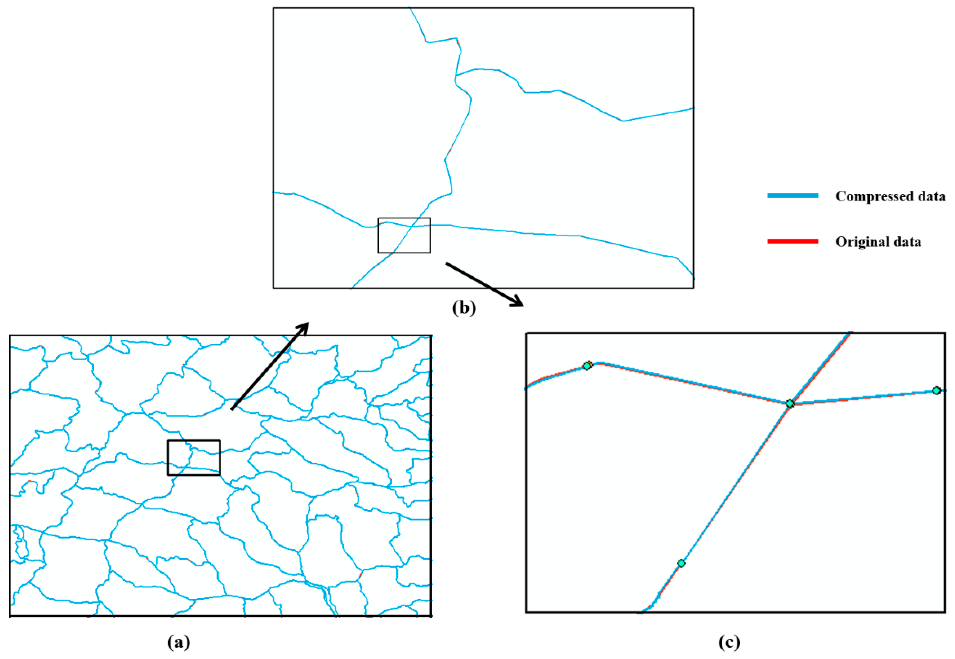
To further compare the performance of this paper’s algorithm, an available algorithm converting floating-point type values to a short integer values is used [20]. As shown in Figure 9, space division level 10 of this paper’s algorithm produces a data rate saving of 97.33%. Furthermore, Li’s method is implemented using parameters Width = 2400 and stepWidth = 2, and the data rate saving is 86.40%. A 1:1 visual comparison of the results of these two compression algorithms is shown in Figure 9.
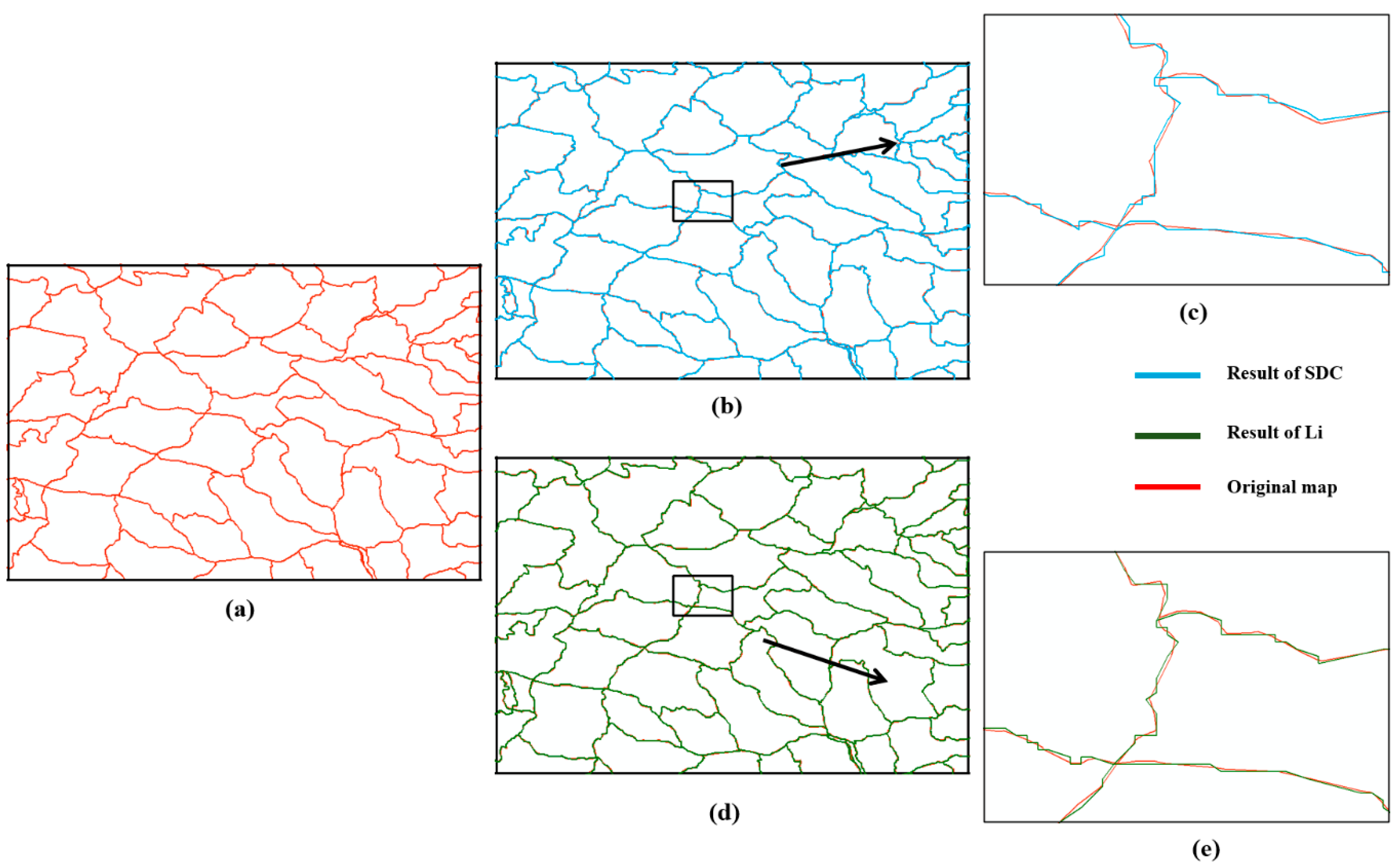
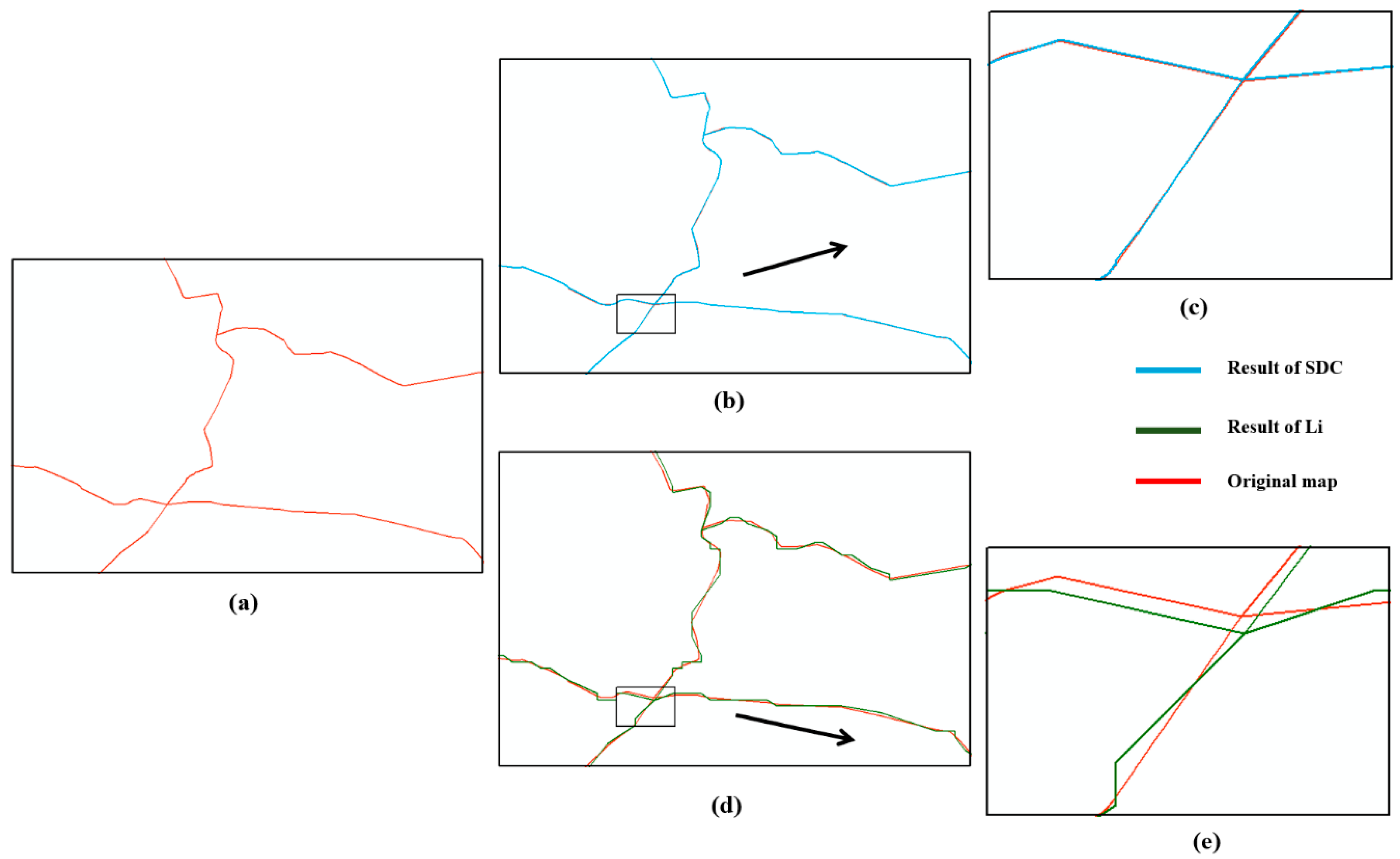
As shown in the Figure 10, space division level 15 of this paper’s algorithm produces a data rate saving of 85.33%. Furthermore, with Width = 3200 and stepWidth = 2, the data rate saving of Li’s method is 83.29%. In addition, the method in this paper maintains better match with the source dataset visually.
4. Conclusions and Discussion
Space division based on Morton and Geohash encoding is mainly used for spatial data index and spatial data management in available studies. Raster data can be compressed with Morton encoding of Quadtrees. This paper proposes and implements a hybrid implementation of Morton and Geohash encoding strategies and applies it for vector data compression. Geographic space is iteratively divided into a regular grid. The center point of each grid cell represented by binary code or binary offset is used to approximate floating-point values of coordinates located in the corresponding cell. This effectively reduces original coordinate storage. This paper implemented a new compression algorithm based on the hybrid encoding strategy. Experiments with four datasets demonstrate that this method is more flexible in space division and offers higher compression efficiency, compared with converting float type values to integer values directly. Multiresolution Morton encoding schemata were implemented and results show that this method is adaptive. This design and implementation for vector data compression can be applied in most real-world situations where vector features are distributed randomly in 2D space. It may not be suitable to use in some extreme situations where vector features are clustered and sparsely distributed, especially for sparsely distributed point features, for which further experiment and evaluation are needed to compare this algorithm’s performance. Error evaluation based on quantitative measures should also be considered in the future.
The lossless compression methods are popular and mostly used for file archiving and quick transmission over network. The experiments in this article shows that lossless compression can achieve 35–75% data rate saving with binary Esri shapefiles. These methods ensure accuracy of vector geometry and can be implemented and accommodated in many applications. However, the corresponding data rate saving is not as significant as the space division-based compression algorithm. Lossless compression may not be applicable when progressive vector data transmission is necessary in the context of quick online visualization, where multiresolution space division encoding results based on this new algorithm are more applicable.
Future research can explore how to implement an algorithm to produce variable length Morton encoding for different nodes of one vector object. A structure can be designed to manage each number of Morton codes in a Level of Details (LODs) manner. A further compression operation using traditional file compression algorithms over encoding results is possible. Further work can include a design of representing encoded results in a JSON format, which can enable spatial data sharing over internet for generic applications [39].
Supplementary Materials
The following are available online at https://0-www-mdpi-com.brum.beds.ac.uk/2220-9964/9/12/721/s1, Figure S1: Test dataset 1: LRDL layer, Figure S2: Test dataset 2: RESP layer, Figure S3: Test dataset 3: gis_osm_natural_free_1 layer, Figure S4: Test dataset 4: gis_osm_roads_free_1 layer.
Author Contributions
Concept presentation, method guidance, original paper writing and revising, Tao Wang; Completion of algorithms, programming and experiments, original draft preparation, Dongge Liu; review and editing, Tao Wang, Xiaojuan Li, Yeqing Ni, Dongge Liu, Yanping Li, Zhao Jin. All authors have read and agreed to the published version of the manuscript.
Funding
This research is supported by a NSFC grant (No. 41671403) and a NKRD program (No. 2017YFB0503502).
Acknowledgments
We are thankful to the reviewers and the editors for their helpful comments and suggestions.
Conflicts of Interest
The authors declare no conflict of interest.
References
- Tao, W. Interdisciplinary urban GIS for smart cities: Advancements and opportunities. Geo-Spat. Inf. Sci. 2013, 16, 25–34. [Google Scholar] [CrossRef]
- Jo, J.; Lee, K.-W. High-performance geospatial big data processing system based on mapreduce. ISPRS Int. J. Geo-Inf. 2018, 7, 399. [Google Scholar] [CrossRef] [Green Version]
- Coluccia, G.; Lastri, C.; Guzzi, D.; Magli, E.; Nardino, V.; Palombi, L.; Pippi, I.; Raimondi, V.; Ravazzi, C.; Garoi, F.; et al. Optical compressive imaging technologies for space big data. IEEE Trans. Big Data 2019, 6, 430–442. [Google Scholar] [CrossRef]
- Li, C.; Wu, Z.; Wu, P.; Zhao, Z. An adaptive construction method of hierarchical spatio-temporal index for vector data under peer-to-peer networks. ISPRS Int. J. Geo-Inf. 2019, 8, 512. [Google Scholar] [CrossRef] [Green Version]
- Feng, B.; Zhu, Q.; Liu, M.; Li, Y.; Zhang, J.; Fu, X.; Zhou, Y.; Li, M.; He, H.; Yang, W. An efficient graph-based spatio-temporal indexing method for task-oriented multi-modal scene data organization. ISPRS Int. J. Geo-Inf. 2018, 7, 371. [Google Scholar] [CrossRef] [Green Version]
- Huang, W.; Yang, J.; Chen, Y.; Zhang, Y.; Zhang, R. Method of vector data compression based on sector screening. Geomat. Inf. Sci. Wuhan Univ. 2016, 41, 487–491. [Google Scholar] [CrossRef]
- Sim, M.S.; Kwak, J.H.; Lee, C.H. Fast shape matching algorithm based on the improved douglas-peucker algorithm. KIPS Trans. Softw. Data Eng. 2016, 5, 497–502. [Google Scholar] [CrossRef]
- Lee, S.; Hwang, W.; Jung, J.; Kwon, K. Vector map data compression using polyline feature. IEICE Trans. Fundam. Electron. Commun. Comput. Sci. 2014, 97, 1595–1604. [Google Scholar] [CrossRef]
- Chand, A.; Vijender, N. Positive blending hermite rational cubic spline fractal interpolation surfaces. Calcolo 2015, 52, 1–24. [Google Scholar] [CrossRef]
- Visvalingam, M.; Whelan, J.C. Implications of weighting metrics for line generalization with Visvalingam’s Algorithm. Cartogr. J. 2016, 53, 1–15. [Google Scholar] [CrossRef]
- Visvalingam, M. The visvalingam algorithm: Metrics, measures and heuristics. Cartogr. J. 2016, 53, 1–11. [Google Scholar] [CrossRef]
- Zhu, F.; Miao, L.; Liu, W. Research on vessel trajectory multi-dimensional compression algorithm based on Douglas-Peucker theory. Appl. Mech. Mater. 2014, 694, 59–62. [Google Scholar] [CrossRef]
- Wang, Z.; Müller, J.-C. Line generalization based on analysis of shape characteristics. Cartogr. Geogr. Inf. Syst. 1998, 25, 3–15. [Google Scholar] [CrossRef]
- Ai, T.; Ke, S.; Yang, M.; Li, J. Envelope generation and simplification of polylines using Delaunay Triangulation. Int. J. Geogr. Inf. Sci. 2017, 31, 297–319. [Google Scholar] [CrossRef]
- Yan, Z.P.; Wang, H.J.; He, Q.Q. A statistical analysis of papers and author group in geomatics and information science of Wuhan University. Adv. Mater. Res. 2014, 998, 1536–1540. [Google Scholar] [CrossRef]
- Xue, S.; Wang, G.; Guo, J.; Yu, W.; Xu, X. Vector map data compression of frequency domain with consideration of maximum absolute error. Geomat. Inf. Sci. Wuhan Univ. 2018, 43, 1438–1444. [Google Scholar]
- Yu, X.; Zhang, J.; Zhang, L. Spatial vector data compression method based on integer wavelet transform. Earth Sci. J. China Univ. Geosci. 2011, 36, 381–385. [Google Scholar]
- Bjørke, J.; Nilsen, S. Efficient representation of digital terrain models: Compression and spatial de-correlation techniques. Comput. Geosci. 2002, 28, 433–445. [Google Scholar] [CrossRef]
- Li, Q.; Yang, C.; Chen, A. Research on geographical relational database model in webGIS. J. Image Graph. 2000, 2, 33–37. [Google Scholar]
- Li, Q.; Liu, X.; Cao, D. Research in webGIS vector spatial data compression methods. J. Image Graph. 2001, 12, 81–85. [Google Scholar]
- Kasban, H.; Hashima, S. Adaptive radiographic image compression technique using hierarchical vector quantization and Huffman encoding. J. Ambient. Intell. Humaniz. Comput. 2019, 10, 2855–2867. [Google Scholar] [CrossRef]
- Ozsoy, A. An efficient parallelization of longest prefix match and application on data compression. Int. J. High Perform. Comput. Appl. 2015, 30, 276–289. [Google Scholar] [CrossRef]
- Isenburg, M.; Lindstrom, P.; Snoeyink, J. Lossless compression of floating-point geometry. Comput. Aided Des. 2004, 1, 495–501. [Google Scholar] [CrossRef]
- Zhang, X.; Chen, J. Fast translating algorithm between QTM code and longitude/latitude coordination. Acta Geod. Cartogr. Sin. 2003, 32, 272–277. [Google Scholar]
- Sahr, K.; White, D.; Kimerling, A.J. Geodesic discrete global grid systems. Cartogr. Geogr. Inf. Sci. 2020, 30, 121–134. [Google Scholar] [CrossRef] [Green Version]
- Google. 2020. Available online: https://github.com/google/s2geometry (accessed on 20 September 2020).
- Uber. 2020. Available online: https://eng.uber.com/h3/ (accessed on 20 September 2020).
- Geohash. 2020. Available online: https://en.wikipedia.org/wiki/Geohash (accessed on 20 September 2020).
- Zhou, C.; Lu, H.; Xiang, Y.; Wu, J.; Wang, F. GeohashTile: Vector geographic data display method based on geohash. ISPRS Int. J. Geo-Inf. 2020, 9, 418. [Google Scholar] [CrossRef]
- Yi, X.; Xu, Z.; Guo, C.; Liu, D. Spatial index structure based on patricia tree. Comput. Eng. 2015, 41, 69–74. [Google Scholar]
- Tang, L.; Da, F.-P.; Huang, Y. Compression algorithm of scattered point cloud based on octree coding. In Proceedings of the 2016 2nd IEEE International Conference on Computer and Communications (ICCC), Chengdu, China, 14–17 October 2016; Volume 2, pp. 85–89. [Google Scholar]
- Gong, X.; Ci, L.; Yao, K. Split-merge algorithm of image based on Morton code. Comput. Eng. Des. 2007, 22, 5440–5443. [Google Scholar]
- Yang, B.; Purves, R.; Weibel, R. Variable-resolution compression of vector data. GeoInformatica 2008, 12, 357–376. [Google Scholar] [CrossRef] [Green Version]
- Samet, H. Applications of Spatial Data Structures; Addision-Wesley: New York, NY, USA, 1990. [Google Scholar]
- Li, Z.; Openshaw, S. Algorithms for automated line generalization1 based on a natural principle of objective generalization. Int. J. Geogr. Inf. Sci. 1992, 6, 373–389. [Google Scholar] [CrossRef]
- OpenStreetMap. Available online: https://www.openstreetmap.org/#map=10/27.1295/31.1133 (accessed on 20 January 2020).
- LZMA. Available online: http://en.wikipedia.org/wiki/Lempel-Ziv-Markov_chain_algorithm (accessed on 25 November 2020).
- Ziv, J.; Lempel, A. A universal algorithm for sequential data compression. IEEE Trans. Inf. Theory 1977, 23, 337–343. [Google Scholar] [CrossRef] [Green Version]
- Ai, T. Constraints of progressive transmission of spatial data on the web. Geo-Spat. Inf. Sci. 2010, 13, 85–92. [Google Scholar] [CrossRef]
Figure 1.
Multilevel space division following a hybrid implementation encoding. (a) is the first-level division grid; (b) is the second-level division grid; (c) is the third-level division grid.
Figure 1.
Multilevel space division following a hybrid implementation encoding. (a) is the first-level division grid; (b) is the second-level division grid; (c) is the third-level division grid.

Figure 2.
Pseudocode of space division algorithm.

Figure 3.
Grid filtering diagram.

Figure 4.
Offset storage of point features diagram.

Figure 5.
Corresponding figure showing line or polygon features offset storage.

Figure 6.
Visualization of compression results at different space division level. (a) is the result of the original data, (b) is the drawing result with a division level of 8, (c) is the drawing result with a division level of 9, and (d) is the drawing result with a division level of 10.
Figure 6.
Visualization of compression results at different space division level. (a) is the result of the original data, (b) is the drawing result with a division level of 8, (c) is the drawing result with a division level of 9, and (d) is the drawing result with a division level of 10.

Figure 7.
Overlaid result of different scale maps when n = 10. (a) is at the display scale of 1:1,000,000; (b) is at the display scale of 1:100,000; (c) is at the display scale of 1:25,000.
Figure 7.
Overlaid result of different scale maps when n = 10. (a) is at the display scale of 1:1,000,000; (b) is at the display scale of 1:100,000; (c) is at the display scale of 1:25,000.

Figure 8.
Overlay result of different scale when n = 15. (a) at the display scale of 1:1,000,000; (b) at the display scale of 1:100,000; (c) at the display scale of 1:25,000.
Figure 8.
Overlay result of different scale when n = 15. (a) at the display scale of 1:1,000,000; (b) at the display scale of 1:100,000; (c) at the display scale of 1:25,000.

Figure 9.
Overlaid results of different scales. (a) is the original map at a scale of 1:1,000,000; (b) is the compression map at the scale of 1:1,000,000 using the new algorithm and n is 15. (c) is the compression map zooming into a scale of 1:100,000 using the new algorithm; (d) is the compression map at the scale of 1:1,000,000 using Li’s method. (e) is the compression map zooming into a scale of 1:100,000 using Li’s method.

Figure 10.
Overlaid results of maps at different scales. (a) is the original map at a scale of 1:100,000; (b) is the compression map at the scale of 1:100,000 using the new algorithm and n is 15. (c) is the compression map zooming to a scale of 1:25,000 using the new algorithm (d) is the compression map at the scale of 1:100,000 using Li’s method. (e) is the compression map zooming to a scale of 1:25,000 using Li’s method.


Table 1.
Binary code of different n.
| n | Bit Length | Binary Code |
|---|---|---|
| 1 | 2 | 01 |
| 2 | 4 | 0110 |
| 3 | 6 | 011010 |
| 4 | 8 | 01101000 |
| 5 | 10 | 0110100001 |
| 6 | 12 | 011010000100 |
| 7 | 14 | 01101000010001 |
| 8 | 16 | 0110100001000111 |
| 9 | 18 | 011010000100011101 |
Table 2.
Point feature binary offset format.
| Starting Point | Offset Point 1 | Offset Point 2 | ||
|---|---|---|---|---|
| 000000000010 | Supplementary bits | Offset bits | Supplementary bits | Offset bits |
| 1010 | 0 | 111 | ||
Table 3.
Line or polygon feature binary offset format.
| Number | Starting Point | Offset Point 1 | Offset Point 2 | ||||
|---|---|---|---|---|---|---|---|
| 13 | 0000000010000001 | Direction bits | Supplementary bits | Offset bits | Direction bits | Supplementary bits | Offset bits |
| 01 | 00 | 01 | 11 | 00 | 11 | ||
Table 4.
Result of precision evaluation.
| n | Bit Length | Number of Rows/Columns | Longitude Resolution (m) | Latitude Resolution (m) | Max_Error (m) | Distance (m) | Magnification |
|---|---|---|---|---|---|---|---|
| 10 | 20 | 1024 | 652.262641 | 585.449125 | 438.2343 | 250 | 0.57 |
| 11 | 22 | 2048 | 326.131321 | 292.724562 | 219.11715 | 250 | 1.14 |
| 12 | 24 | 4096 | 163.06566 | 146.362281 | 109.55857 | 250 | 2.28 |
| 13 | 26 | 8192 | 81.53283 | 73.181141 | 54.779288 | 250 | 4.56 |
| 14 | 28 | 16,384 | 40.766415 | 36.59057 | 27.389644 | 250 | 9.13 |
| 15 | 30 | 32,863 | 20.324284 | 18.242397 | 13.655233 | 250 | 18.31 |
| 16 | 32 | 65,536 | 10.191604 | 9.147643 | 6.8474112 | 250 | 36.51 |
| 17 | 34 | 131,072 | 5.095802 | 4.573821 | 3.4237054 | 250 | 73.02 |
| 18 | 36 | 262,144 | 2.547901 | 2.286911 | 1.7118529 | 250 | 146.04 |
| 19 | 38 | 524,288 | 1.27395 | 1.143455 | 0.855926 | 250 | 292.08 |
| 20 | 40 | 1,048,576 | 0.636975 | 0.571728 | 0.4279632 | 250 | 584.16 |
Table 5.
Compression saving table at different space division n.
| n | Bit Length | RESP.shp | gis_osm_natural_free_1.shp | ||
| Compressed File Size (BYTE) | Data RateSaving | Compressed File Size (KB) | Data Rate Saving | ||
| 5 | 10 | 600 | 98.67% | 17 | 99.89% |
| 6 | 12 | 801 | 98.22% | 30 | 99.81% |
| 7 | 14 | 1206 | 97.32% | 46 | 99.71% |
| 8 | 16 | 1603 | 96.44% | 72 | 99.54% |
| 9 | 18 | 2007 | 95.54% | 122 | 99.23% |
| 10 | 20 | 2409 | 94.64% | 199 | 98.74% |
| 11 | 22 | 2808 | 93.76% | 316 | 97.99% |
| 12 | 24 | 3207 | 92.87% | 473 | 97.00% |
| 13 | 26 | 3613 | 91.97% | 674 | 95.72% |
| 14 | 28 | 4012 | 91.08% | 928 | 94.11% |
| 15 | 30 | 4411 | 90.19% | 1 248 | 92.08% |
| n | Bit Length | LRDL.shp | gis_osm_roads_free_1.shp | ||
| Compressed File Size (KB) | Data Rate Saving | Compressed File Size (MB) | Data Rate Saving | ||
| 5 | 10 | 17 | 99.60% | 4.4 | 98.67% |
| 6 | 12 | 20 | 99.52% | 4.8 | 98.55% |
| 7 | 14 | 28 | 99.31% | 5.1 | 98.46% |
| 8 | 16 | 39 | 99.06% | 5.5 | 98.34% |
| 9 | 18 | 65 | 98.41% | 6.2 | 98.13% |
| 10 | 20 | 109 | 97.33% | 7.1 | 97.85% |
| 11 | 22 | 174 | 95.72% | 8.3 | 97.49% |
| 12 | 24 | 263 | 93.55% | 11 | 96.68% |
| 13 | 26 | 372 | 90.88% | 15.7 | 95.26% |
| 14 | 28 | 491 | 87.95% | 23.1 | 93.02% |
| 15 | 30 | 598 | 85.33% | 32.5 | 90.18% |
Table 6.
Lossless compression results of four test datasets.
| LZMA | LZX | ||||
|---|---|---|---|---|---|
| Data | Original File Size (KB) | Compressed File Size (KB) | Data Rate Saving | Compressed File Size (KB) | Data Rate Saving |
| RESP.shp | 44 | 22 | 50.00% | 25 | 43.18% |
| gis_osm_natural_free_1.shp | 15,752 | 3 906 | 75.20% | 5 372 | 65.90% |
| LRDL.shp | 4075 | 2 248 | 44.83% | 2 610 | 35.95% |
| gis_osm_roads_free_1.shp | 339,477 | 100 850 | 70.29% | 122 226 | 64.00% |
Publisher’s Note: MDPI stays neutral with regard to jurisdictional claims in published maps and institutional affiliations. |
© 2020 by the authors. Licensee MDPI, Basel, Switzerland. This article is an open access article distributed under the terms and conditions of the Creative Commons Attribution (CC BY) license (http://creativecommons.org/licenses/by/4.0/).
Share and Cite
MDPI and ACS Style
Liu, D.; Wang, T.; Li, X.; Ni, Y.; Li, Y.; Jin, Z. A Multiresolution Vector Data Compression Algorithm Based on Space Division. ISPRS Int. J. Geo-Inf. 2020, 9, 721. https://0-doi-org.brum.beds.ac.uk/10.3390/ijgi9120721
AMA Style
Liu D, Wang T, Li X, Ni Y, Li Y, Jin Z. A Multiresolution Vector Data Compression Algorithm Based on Space Division. ISPRS International Journal of Geo-Information. 2020; 9(12):721. https://0-doi-org.brum.beds.ac.uk/10.3390/ijgi9120721
Chicago/Turabian StyleLiu, Dongge, Tao Wang, Xiaojuan Li, Yeqing Ni, Yanping Li, and Zhao Jin. 2020. "A Multiresolution Vector Data Compression Algorithm Based on Space Division" ISPRS International Journal of Geo-Information 9, no. 12: 721. https://0-doi-org.brum.beds.ac.uk/10.3390/ijgi9120721
Note that from the first issue of 2016, this journal uses article numbers instead of page numbers. See further details here.