Quality of GNSS Traces from VGI: A Data Cleaning Method Based on Activity Type and User Experience

Abstract

VGI (Volunteered Geographic Information) refers to spatial data collected, created, and shared voluntarily by users. Georeferenced tracks are one of the most common components of VGI, and, as such, are not free from errors. The cleaning of GNSS (Global Navigation Satellite System) tracks is usually based on the detection and removal of outliers using their geometric characteristics. However, according to our experience, user profile differentiation is still a novelty, and studies delving into the relationship between contributor efficiency, activity, and quality of the VGI produced are lacking. The aim of this study is to design a procedure to filter GNSS traces according to their quality, the type of activity pursued, and the contributor efficiency with VGI. Source data are obtained Wikiloc. The methodology includes tracks classification according mobility types, box plot analysis to identify outliers, bivariate user segmentation according to level of activity and efficiency, and the study of its spatial behavior using kernel-density maps. The results reveal that out of 44,326 tracks, 8096 (18.26%) are considered erroneous, mainly (73.02%) due to contributors’ poor practices and the remaining being due to bad GNSS reception. The results also show a positive correlation between data quality and the author’s efficiency collecting VGI.

1. Introduction

VGI (Volunteered Geographic Information) refers to spatial data that are voluntarily collected, created, and shared by users [1]. VGI constitutes large series of data, which can be used for a variety of purposes [2,3,4,5,6]. Overall, VGI is considered a highly valuable and innovative data source in geographical research [7]. Among the many advantages offered by VGI, it is free, it provides a large amount and continuity of data, and information is made available that was never previously used on a spatial basis [8]. VGI also presents many challenges [8,9], among which the following are of note: (1) its quality is highly variable and is undocumented; (2) when it is generated, the scientific principles of collecting geographic data are rarely followed; (3) its authors are not professionals, so they do not have the same training or commitment as professionals in the process of acquiring data; and (4) in many cases, data present varying levels of detail because they have been captured via different methods or devices. Of all these issues, the quality and reliability of data stand out [10].

Georeferenced tracks are one of the most common components of VGI and, as such, are not free from errors [11,12]. Many studies have been conducted on the pre-processing of data from VGI GNSS (Global Navigation Satellite System) traces. Notable examples were published [12,13,14,15,16], which mainly focused first on detecting outliers to then correcting or removing them. The most common geometric errors related to capturing data with GNSS devices occur due to factors that influence the quality of the signal such as ionospheric and atmospheric delays, the multipath effect (when the receiver is located near a reflective surface), or the dilution of accuracy [11]. However, when GNSS data from VGI are processed, such errors are not always the most relevant: although they distort the GNSS signal, those caused by the users are the most common. This is because the incorrect use of the application causes significant errors that considerably alter or deform GNSS traces. Two main error sources can be identified regarding GNSS data quality: (1) those resulting from the capture device and (2) those caused through misuse of the VGI platform used by the contributor. Although the first source of error may greatly distort the process of capturing a GNSS path, the second, corresponding to the user’s good practices, not only affects the thematic attributes of the traces but also their geometry [12].

The cleaning of GNSS tracks is based on the detection and removal of outliers to evaluate their intrinsic spatial quality and avoid using anomalous traces. An outlier in a GNSS trace may be defined as an x,y point or coordinate whose metric and geometric characteristics differ significantly from the characteristics of other points or coordinates that compose the complete trace [11,12]. Some authors e.g., [15] used the geometric characteristics of the components of the traces to detect and analyze outliers. They drew from the premise that a continuous sequence of points (coordinates) or segments of a trace with a significant deviation from the main sequence of GNSS traces will determine an atypical section of the trace in question. Other studies [13,14] applied data pre-processing methods using all their components, including the temporal component. Thus, they identified the noise of traces with a space–time cube depending on the shape, speed, and topology of the segments that composed the trace.

Contributors to VGI have a variety of backgrounds and their motivations to collect and share data may also be diverse [17]. One of the main methodological challenges faced by VGI is related to user profile heterogeneity [18]. Behind a common desire to share with others, different users have different motivations and behave in different ways. An instance was previously provided [19]; the authors analyzed off-trail rambling through a variety of sportive apps, finding that off-trail practices were twice as prevalent among cyclist than among runners. Along this line, a group of works focused on differentiating user profiles according to several areas and themes e.g., [20,21,22,23]. Most works focused on the type of activity users perform e.g., [19]. However, works analyzing the role of VGI contributor in terms of efficiency in data collection are lacking. To the best of our knowledge, user profile differentiation according to contributor efficiency is still poorly understood, and works examining the relationship between contributor’s efficiency, activity, and quality of VGI produced are scarce. A notable exception is [24], which aimed at assessing data quality with regards to contributor reputation among users within a given platform. Another significant exception is [25], which associated trustworthiness of information and author’s reputation in the approach to VGI quality, finding that those parameters can be used as quality indicators. Despite some recent works, the role of the contributor’s background in data collection has not been sufficiently explored.

It is understood that the contributor’s background includes experience and efficiency. An experienced contributor would be more competent in the use of VGI-related devices, platforms, and procedures, and hence would prove more efficient in producing better outputs. By acknowledging contributor efficiency, it is assumed that the contributor’s practical knowledge plays a significant role in their competence. The aim of this study was to construct a procedure to filter GNSS tracks according to their quality, the type of activity pursued, and the contributor’s efficiency with VGI. We hypothesized that users behave differently according to the activity they perform, that more experienced VGI users tend to be more efficient than less experienced users, and that activity and efficiency affect the final reliability of the information. Our goals were to: (1) detect and clean spatial errors in a GNSS database, and (2) characterize users according to their activity and efficiency. The study was conducted within the peri-urban setting of Tarragona (Spain) and Wikiloc tracks were used as the VGI source.

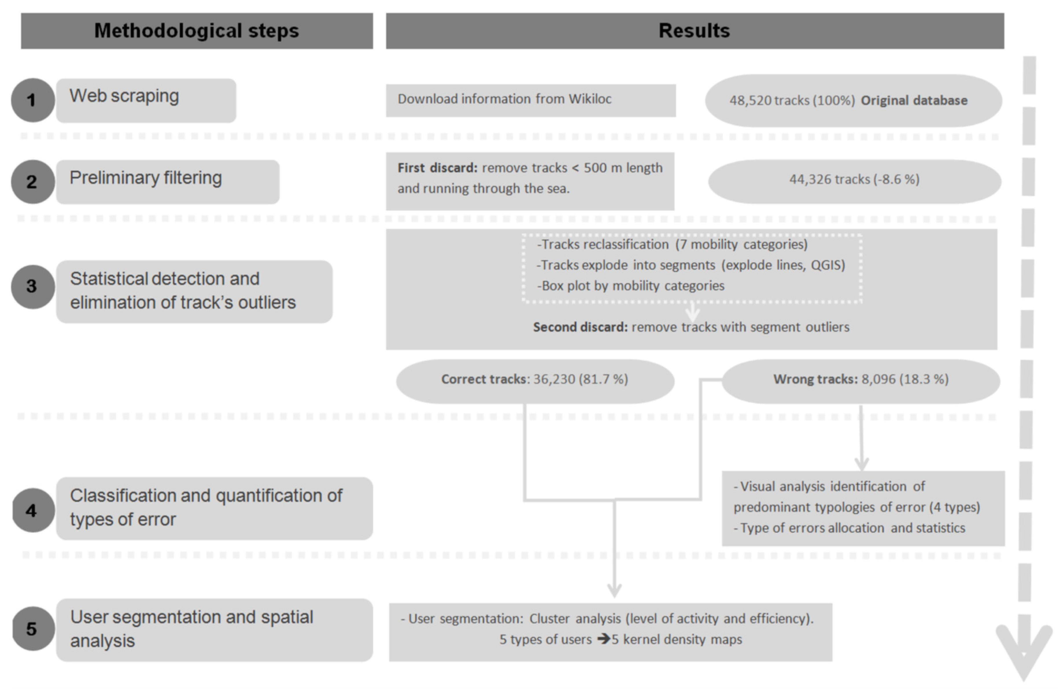
2. Materials and Methods

The devised methodology is split into five steps: (1) web scraping or the downloading of massive data, (2) preliminary filtering, (3) statistical detection and elimination of tracks with segments understood as outliers, (4) classification and quantification of types of error in the removed tracks, and (5) segmentation of users and analysis of spatial behavior. Figure 1 shows the different steps of the procedure and the results associated with each step.

2.1. Source, Web Scraping, and Database Characteristics

The VGI data for this study were directly obtained from the Wikiloc web platform: a crowdsourced online platform operating since 2006 [26]. This online service allows the sharing of outdoor tracks that can be supplemented with georeferenced photographs. In 2020, it reached more than 5 million users worldwide with more than 15 million tracks shared and 27.5 million photographs. Tracks can be recorded using all kinds of GNSS devices and smartphones, and can be uploaded to the platform via an Internet connection immediately after being completed.

Data were downloaded using web scraping techniques and a geodatabase was set up consisting of a spatial file containing geometric information about the tracks (.kml) and another theme with their attributes (.csv). The thematic information associated with the tracks features the following fields: author/user, activity carried out, URL of the track, downloads received, date recorded, recording device, and whether the track is circular or not.

The .kml file obtained by web scraping contains the generalized or simplified tracks, i.e., the number of vertices is less than that of the original tracks with the .gpx extension. In addition, the time variable that can be used for their debugging is not associated with them. If the tracks are downloaded manually, their evolution in time can be retained; however, the temporal attribute is lost when data are exported to work formats, which prevents applying certain methodologies [13,14,16].

2.2. Preliminary Filtering

The debugging process begins with preliminary filtering to (1) discard the tracks less than 500 m in length considered functional tests performed by the user or itineraries expressly recorded that are not representative of the set and (2) remove the tracks wholly or partly in the sea, since our focus was terrestrial tracks. In both cases, these tracks do not provide substantial information to the database, either spatially or thematically, and it was deemed appropriate to discard them.

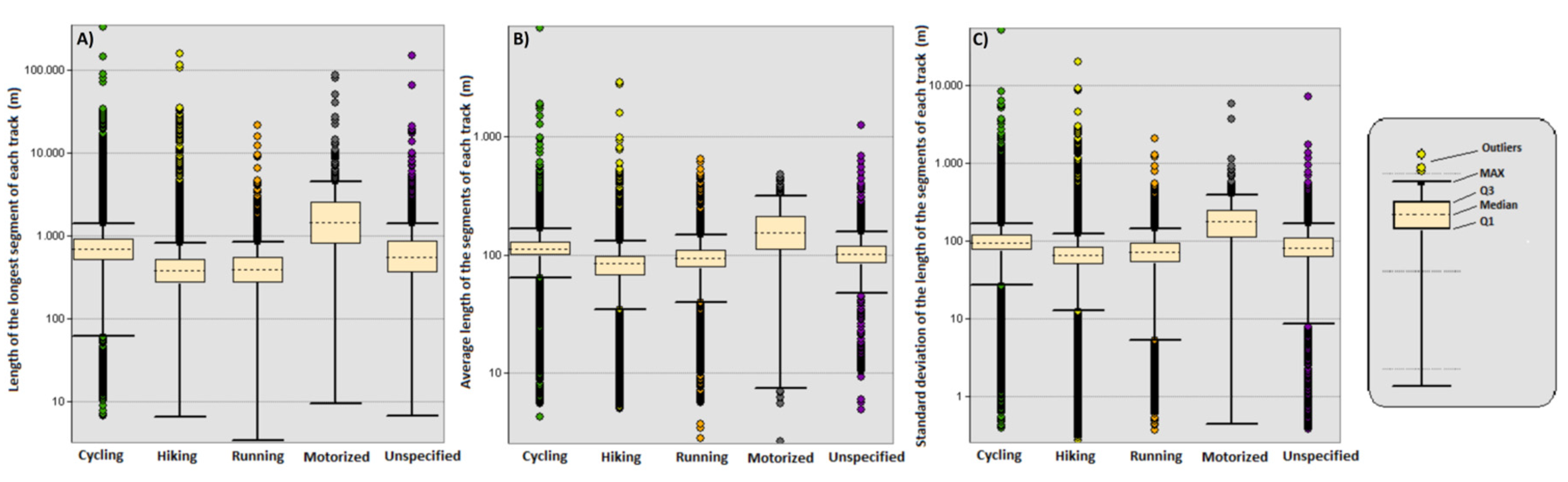
2.3. Statistical Analysis for the Detection and Removal of Outliers

Detect statistically atypical traces within the set of tracks of the same activity is considered more effective than from all tracks, without distinguishing which type. For example, a track of 180 km in length would be an outlier in the “hiking” but not in the “motorized” category. For this reason, the 32 detected activities from Wikiloc were reclassified into seven categories based on type of mobility (

Table 1. Reclassification of Wikiloc activities in mobility typologies.

Type of Activity in Wikiloc (Old Category)	Type of Mobility (New Category)	Type of Activity in Wikiloc (Old Category)	Type of Mobility (New Category)
Cycling (unspecified)	Cycling	Car	Motorized
Mountain bike		Motorcycle
Bicycle touring		Quadricycle
Trail bike		Recreational Vehicle
Gravel bike		Trial motorcycle
Enduro		Skating (unspecified)	Skating
Downhill mountain biking		Skating (line skates)
eBike		Electric scooter
Trailer bike		Horseback riding trail
Trekking/hiking (unspecified)	Hiking	Mountaineering	Others
Nordic walking		Training
Orienteering races		Multisport
Via ferrata		Spelunking
Hiking (with baby stroller)		Birdwatching
Canyoning		Unspecified	Unspecified
Running (unspecified)	Running
Running (on trails)
Canicross

).

Then, each of the traces was exploited to obtain the segments that compose them with the Explode Lines algorithm of QGIS (free software). Once the traces were segmented, for each trace, the following were calculated: (A) the length of the longest segment, (B) the average length of the segments, and (C) the standard deviation of the length of the segments. For each of these variables, a box-and-whisker plot was generated to identify traces with atypically long segments within the activity group to which they belonged. In this type of graph, outliers are those that are above the max value (the third quartile + the interquartile range: Q3 + IQR) and below the min value (the first quartile – the interquartile range: Q1 – IQR). In this case, an atypically short segment of the track may be related to a high GPS sampling frequency and does not show any type of error in the track. The presence of one or more atypically long segments in a track means that there are errors in its geometry. Therefore, only erroneous tracks that had one or more segments with a length greater than the max value were considered.

2.4. Visual Analysis for the Characterization of Errors and Identification and Allocation of Error Types on Discarded Tracks

To identify and characterize the most common errors, the tracks were visually analyzed to detect the very long segments that are largely responsible for the noise present in the dataset. In addition, the causes of each characterized error and whether the cause was the user or the device was identified. This visual analysis allowed identification of a total of four different types of errors (A, B, C, and D), which are described and explained in Section 3.2.

Due to the difficulty of quantifying the types of error of the set of erroneous tracks, an estimate was performed with a random sample. For this calculation, the QGIS Random Selection algorithm was applied to extract a random sample of 30% of the discarded tracks. Therefore, from the total set of discarded tracks (8096), a sample of 2428 tracks (30%) was selected for visually analysis by assigning each track one of the four types of errors previously defined. This step was conducted manually by means of visual inspection by a trained cartographer. The erroneous tracks were classified into one of the four types of errors previously defined, in addition of a fifth one called “other types”.

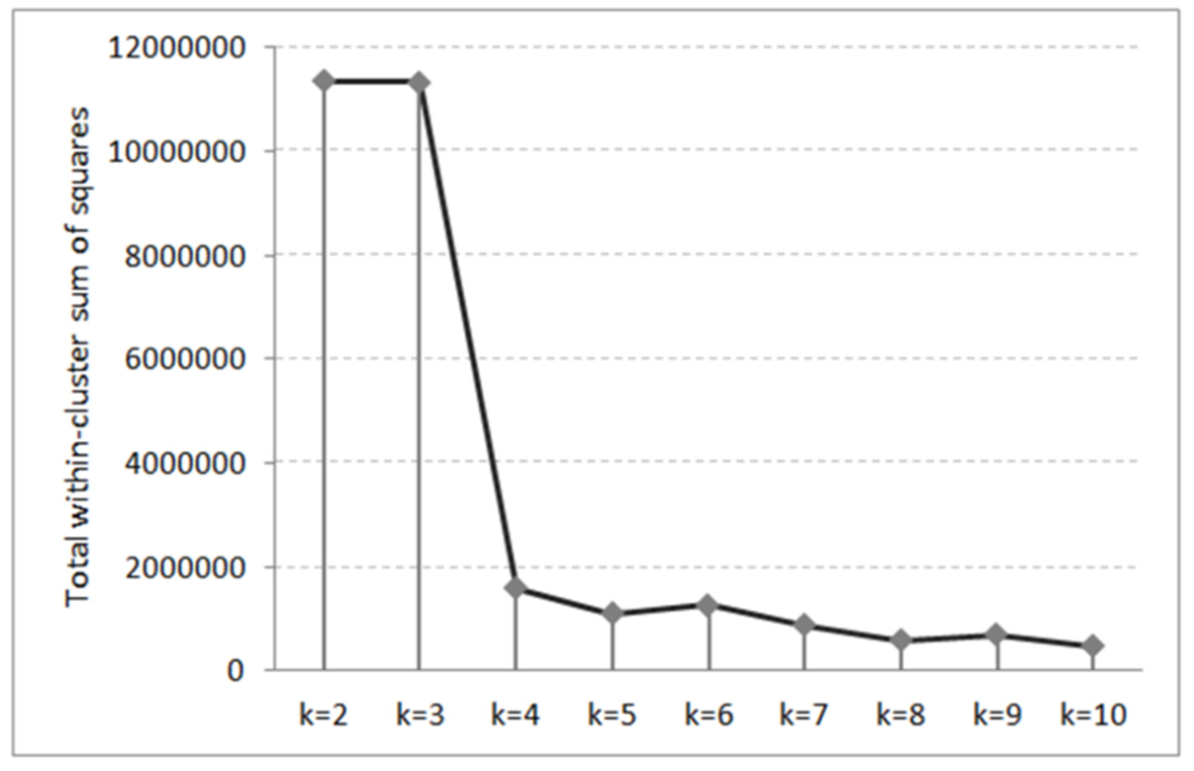
2.5. Segmentation of Users and Spatial Analysis

Having identified the erroneous/correct tracks, for each user, the following were calculated: (1) the proportion of correct tracks over the total number of tracks shared by each user (percentage of “correct tracks”) and (2) the total number of tracks shared on Wikiloc, which are variables used in the cluster analysis based on k-medians clustering to classify users into types according to their degree of expertise. This bivariate model means that the higher the percentage of correct tracks (high efficiency) and the greater the number of tracks shared (high activity), the greater the user expertise or reliability.

This method is a variation of k-means clustering where instead of calculating the mean of each group to determine its centroid, the median is calculated. The median is considered a more robust measurement than the mean, since it is not influenced by outliers. In the case of k-medians, Manhattan distance was used instead of squared Euclidean distance (k-means) as a dissimilarity measure [27]. In summary, considering the distribution of the analyzed data, characterized by the presence of outliers, more robust results were obtained to determine the cluster center using the median.

To select the optimal number of clusters, the algorithm was repeated nine times, testing from 2 to a total of 10 clusters. In each test, the total within-cluster sum of squares (WSS) was calculated, following the work of others [28,29]. According to the Elbow Method [30], the point at which an abrupt change (“elbow”) is observed in the WSS value is considered indicative of the appropriate number of clusters to be selected for the data range in question [31,32]. Figure 2 shows that the WSS decreases as k increases and an abrupt curve or elbow can be easily identified at k = 4. Although according to this method k = 4 should be selected, it was decided to select k = 5 because a new cluster appears whit it, which is associated with an intermediate user profile.

For spatial analysis, it was conducted a track density analysis. In this sense, a kernel-density analysis was conducted on the tracks for each type of user. The resulting rasters had a cell length of 100 m and were classified into four levels of frequentation or intensity of use based on Jenks’ natural breaks method to obtain groups with homogeneous values within the series: 0, 1, 2, 3 (from lower to higher density, respectively). The representation of the five density maps (Section 3.4) used the same classification by intervals in each so that they could be compared with each other.

2.6. Study Area

The study was conducted in a peri-urban area comprising the municipality of Tarragona (Catalonia, Spain) and surroundings (Figure 3). It covers an area of 21,871 hectares with a total population of 289,723 in 2019 [33] and two major population centers (Tarragona and Reus), plus other smaller settlements and shopping and entertainment centers that are arranged around them.

This area is arranged along the coastline in the southeast, and follows the course of the Francolí River, which flows from north to south and divides the study area into two: west and east. In this setting, the traditional agricultural landscape has been fragmented due to the proliferation of industrial, logistics, and commercial areas along with the presence of a dense network of infrastructure. As a result, it appears chaotic with the emergence of many interstitial spaces between the communications networks, the peri-urban neighborhoods, and the commercial and industrial areas [34]. Despite this accumulation of functions, this space has the potential for recreation and conducting activities outdoors as it has an extensive network of tracks and trails, some recognized by the Spanish Federation of Mountain Sports and Climbing (FEDME).

The Wikiloc social network is rather popular in this area and other studies have used it as a source of VGI in places nearby [5,6,18].

3. Results

The results obtained are presented from the perspective of data pre-processing and the analysis of users. The pre-processing of tracks includes the types of errors present and their characteristics according to type of activity. The analysis of users includes their reliability and spatial behavior.

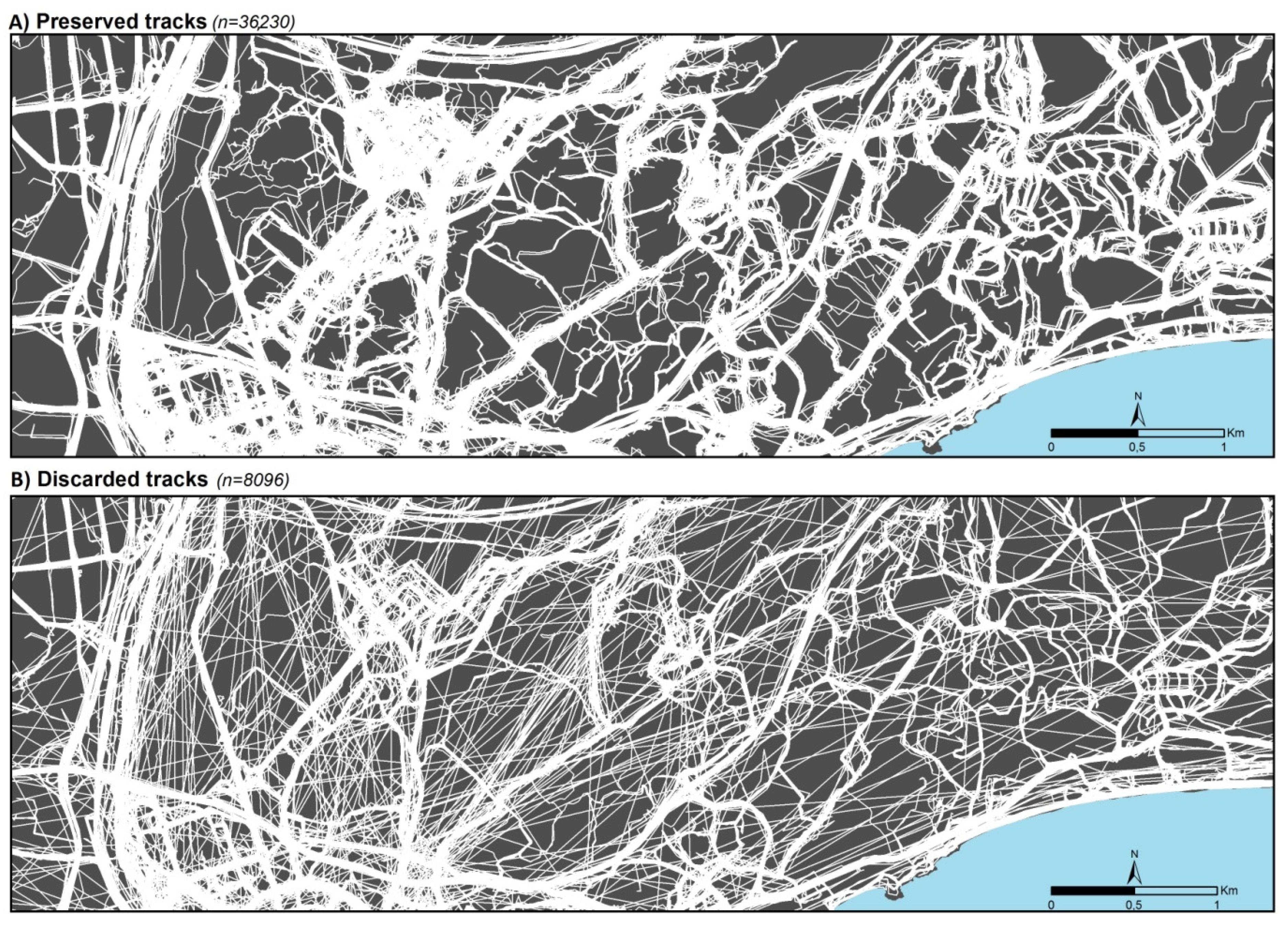
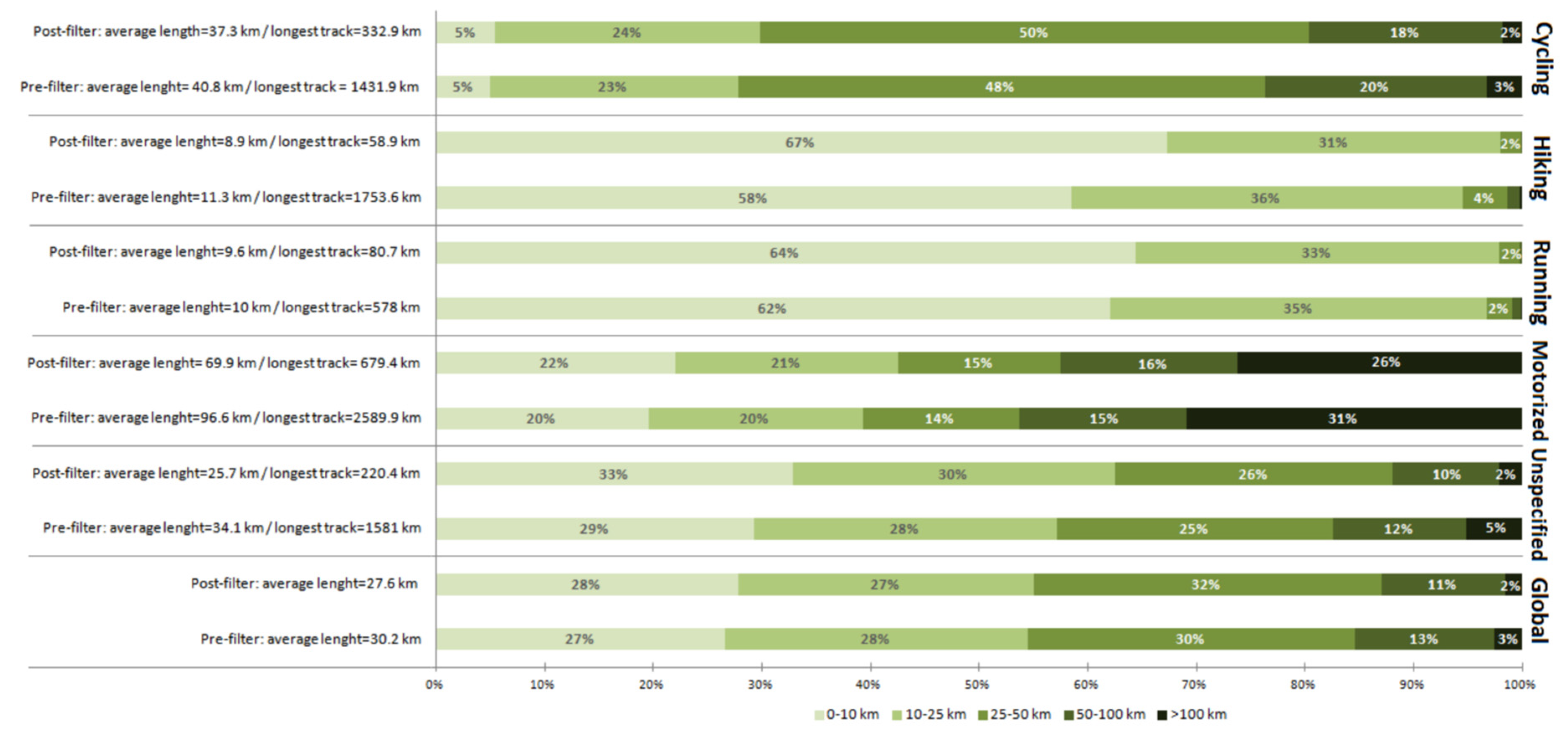
3.1. Pre-Processing and Filtering: Characteristics of Discarded and Preserved Tracks According to Mobility Type

In the first preliminary filter step corresponding to the removal of tracks with of less than 500 m (Section 2.2), 0.5% of GNSS traces were discarded (from 48,520 to 48,279), and in the second, to discard non-terrestrial tracks, 8.2% were removed, reducing the number of tracks from 48,279 to 44,326.

The set of 44,326 tracks resulting from preliminary filtering underwent division into segments and subsequent statistical analysis by box-and-whisker plots (Section 2.3) constructed for each variable and by activity groups (Figure 4). In them, outliers were considered to be those greater than the max (unusually long segments): box upper whisker was calculated from the sum of the third quartile and the interquartile range (Q3 + IQR). The algorithm used to select the correct traces was: A <= Max (A) AND B <= Max (B) AND C <= Max (C), which was applied for each type of activity (

Table 2. Max values that were used to determine the tracks with outliers (atypically long segments) by type of activity and for the three variables analyzed: (A) length of the longest segment of each track; (B) average length of the segments of each track; (C) standard deviation of the length of the segments of each track.

Activities	A: Length of the Longest Segment of Each Track	B: Average Length of the Segments of Each Track	C: Sd of the Length of the Segments of Each Track
	Max Value (m)	Max Value (m)	Max Value (m)
Cycling	1395.09	166.44	169.41
Hiking	495.15	131.64	122.93
Running	853.30	149.03	143.27
Unspecified	1411.31	157.78	165.65
Motorized	4508.78	315.70	394.77

). This method of debugging retained a total of 36,230 tracks (81.7%), removing 8096 tracks (18.3%).

Figure 5 compares the tracks considered correct and those that were discarded. The first case (Figure 5A) highlights its spatial logic, and they are represented in branch fashion with the typical capillarity of the road network. The second case (Figure 5B) highlights the unusual geometry of the tracks and their lack of territorial sense. In Figure 5A, entities that at first glance seem not to follow a logical geometry are highlighted, as they may be associated with errors in some segments. These long and straight lines were not identified by the filter algorithm as statistically anomalous segments because most of them refer to bicycle or motorized tracks in which the algorithm was less restrictive. Random analysis of tracks that visually still contained errors (n = 50) revealed that 62% correspond to the cycling category, 16% to motorized tracks, and the remainder (22%) to other activities.

Over half of the original tracks were created by bicycle; consequently, the highest percentage of discarded tracks corresponded to this activity. Activities on foot (hiking and running) accounted for 37.3%, while the remaining activities displayed little significant weights.

From the group of discarded tracks, 17.4% corresponded to tracks created through the three main activities (cycling, hiking, and running), and this proportion was divided almost equally between those on bicycle or on foot (8.3% and 9.1%, respectively). Finally, the percentage of discarded tracks of other activities accounted for a mere 0.9% altogether (

Table 3. Type of selection and number of tracks before and after filtering by activity groups.

Activities	Tracks Pre-Filter	Tracks Pre-Filter (%)	Type of Selection of the Correct Tracks	Preserved Tracks	Discarded Tracks	Discarded Tracks (%)
Cycling	25,310	57.10	Selection algorithm	21,611	3699	8.34
Hiking	10,644	24.01	Selection algorithm	7348	3296	7.44
Running	5889	13.29	Selection algorithm	5145	744	1.68
Unspecified	1675	3.78	Selection algorithm	1415	260	0.59
Motorized	680	1.53	Selection algorithm	590	90	0.20
Skating	67	0.15	Visual check and manual selection	63	4	0.01
Others	61	0.14	Visual check and manual selection	58	3	0.01
Total	44,326	100	-	36,230	8096	18.26

).

Many of the erroneous tracks featured unusually long segments that considerably increase their real length. Figure 6 shows that the mean and maximum distance of the tracks were larger before applying the filter and that the maximum length of each type of activity reduced after debugging. For example, the longest hiking track before processing was almost 2000 km, which was 59 km after the cleaning procedure. This situation was common to all other activities, with the longest track length being consistent with reality after debugging.

If track lengths were analyzed by intervals in all activities, the proportion of tracks with a length greater than 100 km decreased due to the removal of tracks with unusually long segments.

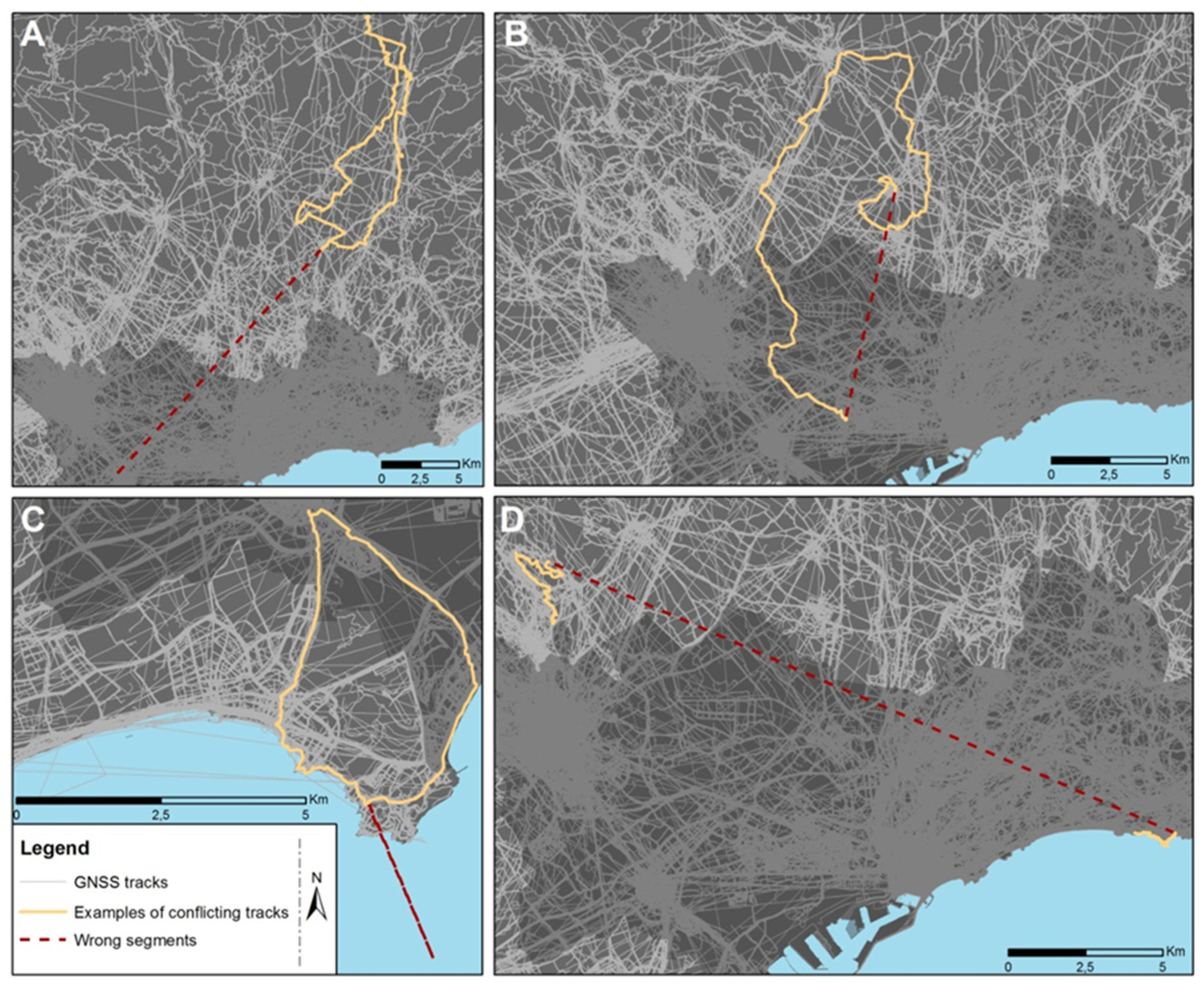
3.2. Types of Errors on Tracks

Regarding the discarded tracks, four predominant types of errors were identified by visual analysis (Section 2.4). Of these four types, three are associated with errors caused by users and the other is related to GNSS device signal quality:

A: Long, straight segments between the penultimate and last vertex of the itinerary. This error is associated with the misuse of the application. The problem segment is generated when “track” is paused and the user resumes at a location distant from the actual end (e.g., at home). As shown in Figure 7A, a straight trace appears that joins the last point of the track (where there is a pause) and the point where track is uploaded to the platform for sharing.

B: Long, straight segments between the vertices of each end of the itinerary. This error may also be directly associated with the user and is generated at the time of ending “track” and it prompts the application that a circular itinerary has been completed when this is not the case. Wikiloc generates a straight line between the two ends of the track to make it into a circular path and fully close it (Figure 7B).

C: Loss of GNSS signal. Errors due to the quality of the signal generating very long segment pairs in any section of the trace (Figure 7C).

D: Long, straight segments between the end vertex of an itinerary and the start vertex of another, completely different one. This error is associated with the use of the application and occurs because the user pauses the recording, having finished a track, by starting another continuous one adding coordinates to the previous track (Figure 7D).

Each trace of a random sample of 30% of the discarded tracks (2428 tracks of the total 8,096 tracks discarded) was associated with a particular type of error (Section 2.4). The results showed that 31.01% of the erroneous tracks correspond to error type A, 33.03% to type B, 22.98% to type C, 8.98% to type D, and the remainder (4%) were not classified because they were attributed to other, uncategorized errors.

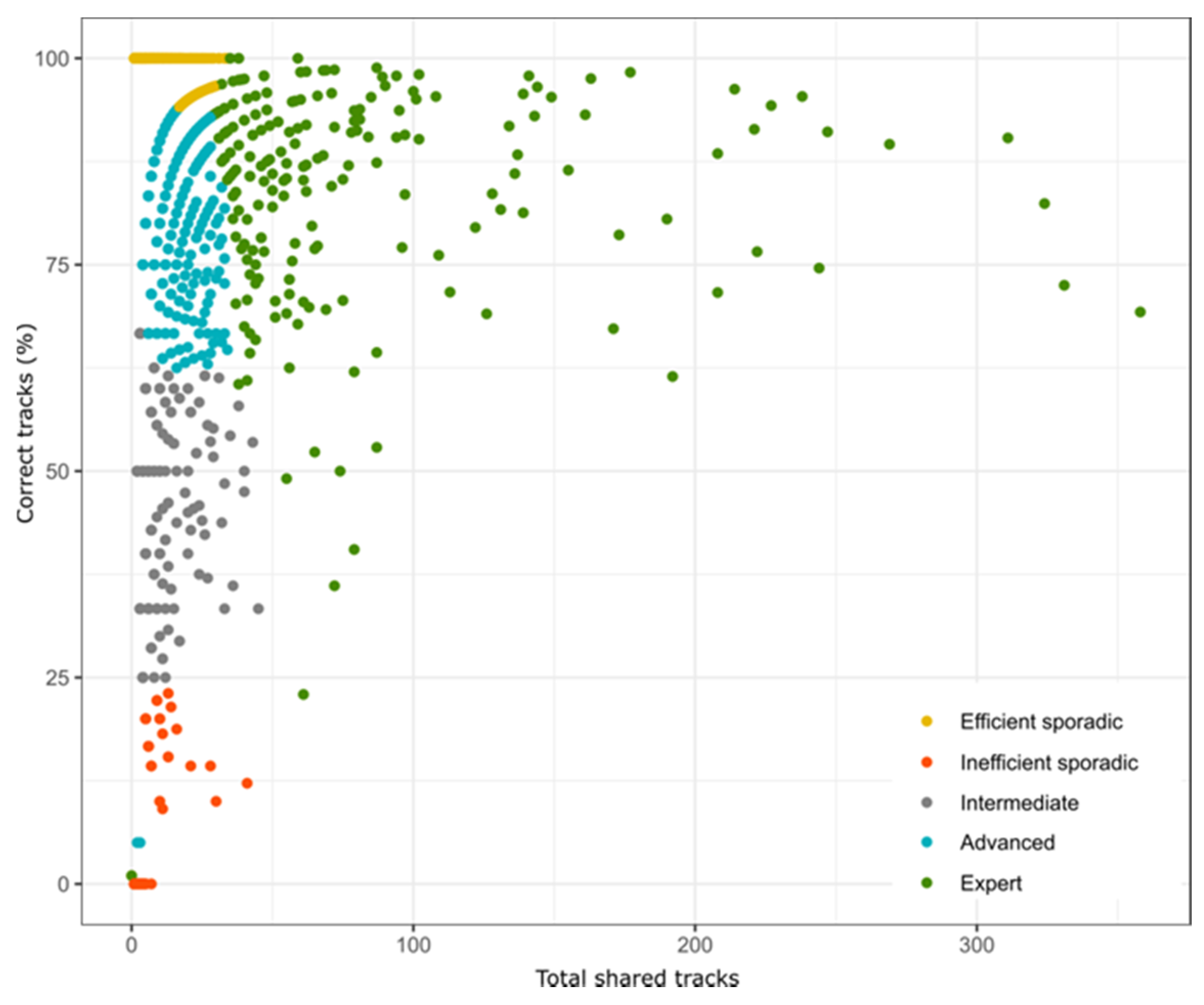
3.3. Reliability of Users

After applying the cluster analysis (Section 2.5), five profiles or different types of user were described, depending on their level of activity and efficiency (percentage of correct tracks) (

Table 4. Centroids of k-medians clustering (5 clusters), assigned level of activity or efficiency and user typologies established by each k.

Clusters	Total Shared Tracks (n)	Correct Tracks (%)	Activity Level	Efficiency Level	User Type
	Cluster Centroid (Median)	Cluster Centroid (Median)
k1	1	100	Very low	Very high	Efficient sporadic
k2	1	0	Very low	Very low	Inefficient sporadic
k3	3	50	Low	Medium	Intermediate
k4	9	80	Medium	High	Advanced
k5	56	88	Very high	Very high	Expert

, Figure 8). The first and second profiles, k1 and k2, are characterized by a very low number of tracks shared on Wikiloc (one track according to the median); however, whereas the first type (k1) presents very high efficiency, that of the second (k2) is very low (median percentage of correct tracks = 0). For this reason, the first has an “efficient sporadic” profile and the second has an “inefficient sporadic” profile. The three following groups highlight that the higher the number of tracks, the higher the percentage of correct tracks, from which it follows that experience and efficiency are positively correlated. Therefore, k3 is an intermediate-type user (low activity and medium efficiency), k4 has an “advanced” profile (average activity and high efficiency) and, finally, k5 corresponds to the “expert” user type (very high activity and efficiency).

The group with the largest number of users is the efficient sporadic group, with 62% of the total (

Table 5. Proportion of users, shared and correct tracks by user types.

User Type	Users		Tracks
	n	%	n	%	Preserved	Discarded	% Correct
Efficient Sporadic	4814	62.00	12,115	27.34	12,071	44	99.64
Inefficient Sporadic	1013	13.05	1553	3.50	59	1494	3.80
Intermediate	850	10.95	4224	9.53	2124	2100	50.28
Advanced	872	11.23	9800	22.11	7912	1888	80.73
Expert	216	2.78	16,627	37.52	14,056	2572	84.54
Total	7765	100	44,319	100	36,222	8098

). The rest is spread in rather even percentages of between approximately 10% and 13%, except the expert group, which did not reach 3% of total users (2.78%). Therefore, most users are sporadic (75%), indicating that they shared a very low number of tracks in the study area. Conversely, the more reliable users (advanced and expert) shared a greater proportion of tracks (59.63%) with a very high percentage of correct tracks (80.73% and 84.54%, respectively). At the other end of the scale is the inefficient sporadic user, who shared the fewest tracks (3.5%) and simultaneously produced the lowest percentage of correct tracks (3.8%). Finally, intermediate users shared about 10% of the total tracks (9.53%) and their percentage of correct tracks was around half (50.28%).

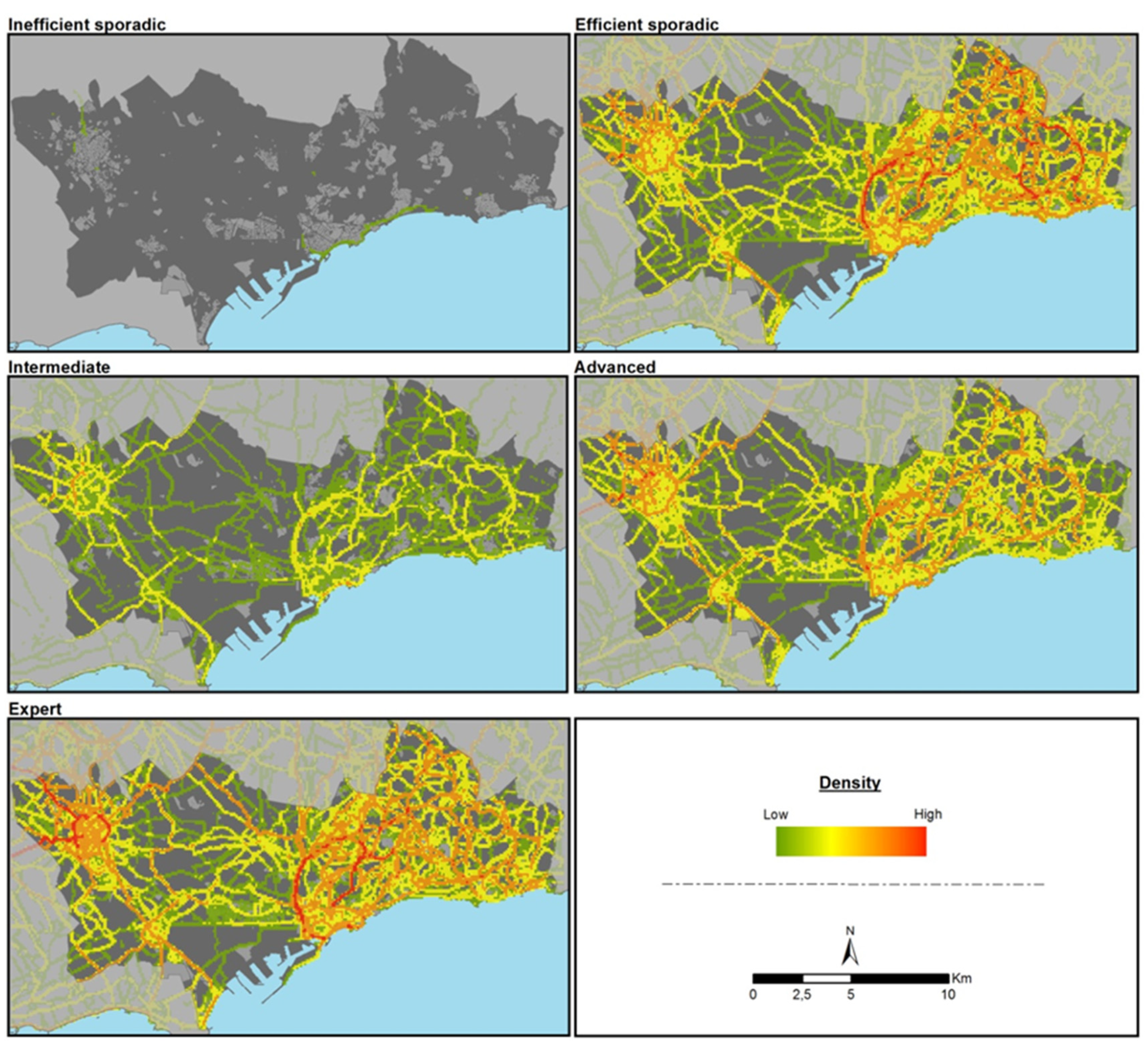
3.4. Spatial Behavior of Users According to Their Level of Efficiency, Expertise, or Reliability

The higher the density of tracks, the more a place is frequented. Thus, using a kernel-density analysis of tracks, highly frequented axes according to user type were readily identified (Figure 9). From the heat map of inefficient sporadic users, the coastal axis of the municipality of Tarragona was observed as being highly frequented from the port to the coastal residential developments within the municipal district. Efficient sporadic users move mainly along the axis of the Francolí River and inland sections that connect small settlements. Intermediate users more intensely frequent the periphery of Reus, the axis of the Francolí River, and the coastline of Tarragona. Advanced and expert users produced an almost identical spatial pattern and their mobility also focused around the periphery of the town of Reus, the axis of the Francolí River, and the inner axis of the municipality of Tarragona.

4. Discussion

This article presents a methodology for debugging GNSS data taken from VGI by detecting unusually long segments in groups of tracks classified according to the performed activity. In addition, this filtering allows dividing the set of traces into preserved (no outliers detected) or discarded/removed (outliers present), which enables the later segmenting of users according to their degree of reliability.

Studies [11,15] have determined outliers from the length of each trace, the number of vertices, the standard deviation, and the maximum Z distance above the digital elevation model, but did not differentiate between the type of activity or the features of the recorded track. A key step in the method proposed here is the separation of tracks by type of activity. Tracks have different geometric features according to the type of activity recorded, and the length of a segment considered unusual varies according to the activity. Therefore, the tracks should be analyzed according to the type of activity rather than without distinguishing between types. Furthermore, the algorithm applied is most advantageous when processing large volumes of geographic data, assuming visual analysis is not feasible to discard erroneous tracks.

The techniques used to debug such data rely to some extent on their characteristics, which are the format of the layer containing the tracks and their thematic attributes that may influence filtering methods. For example, some formats, such as .gpx, can record the time variable, although this is lost when data are obtained in .kml format. This point is significant because it limits the versatility of the most popular data extensions such as Google’s .kml. Some procedures attach importance to the temporal variable of traces: Ivanovic et al. [16] designed a method that considers the speed at which the tracks are covered to then manually tag a sample of atypical and non-atypical values and end with the application of an algorithm to detect irregularities; others [13,14] also used the time component with a space–time cube depending on the shape, speed, and topology of the segments, and associated rather unrealistic speeds with the presence of errors.

From the original set of tracks, 18.3% of the traces were removed. Although this might a priori seem to be a dismissal of a considerable amount of information, it is similar to the value reported in other studies. Usyukov [35] removed about 10% of the original data; Bergman et al. [36] started with a total of 29,958 tracks, but discarding 22% of the total original data, resulting in 23,290 tracks.

The assignment of the sample of discarded tracks into the predefined types of error was conducted by a trained cartographer by means of visual inspection. In this sense, it is assumed that different technicians may produce different results depending on their interpretation of the tracks with erroneous segments. However, we speculate that this estimate would not change significantly because the four predominant types of error are easily distinguishable from each other through a simple visual analysis.

Statistical analysis of the length of the tracks before and after processing as well as the preserved and discarded track map confirmed that the degree of operability and reliability of spatial data after debugging have considerably increased, also demonstrating the superiority of this method over simple visual inspection.

Notably, the algorithm functions to identify the entities with atypical segments within the same activity group and according to the contributor’s efficiency. Therefore, the set of spatial data does not remain completely free of errors and some preserved tracks may still have erroneous segments that were not considered statistically atypical. However, this should not be considered a problem as the goal is to remove most of the noise generated by tracks with very long segments lacking territorial sense to retain an operational database.

5. Conclusions

In this study, a method of filtering to detect and discard GNSS traces with errors from Wikiloc was developed. Boxplots were used to identify outliers, and quality filtering was ensured using the statistical processing of the tracks according to activity groups and considering contributor efficiency.

Of all the tracks, 18.3% were discarded, mostly due to problems related to misuse by the user (73.02%). Fewer problems were related to a loss of signal by the GNSS device (22.98%). Our experience suggests that the number of discarded tracks may be a good indicator for evaluating the quality of a VGI source, and that a threshold of acceptable quality may be at around 20% of discarded tracks [35,36,37].

The statistics of the length of tracks according to activity before and after debugging showed how the proposed method is able to adjust the data to maintain values that are closer to reality. As such, excessively long tracks (due to the presence of erroneous and atypically long segments) for the type of activity performed are eliminated.

The proposed procedure enables the differentiating of five types of users based on their efficiency. More efficient users record more tracks and produce fewer errors. This leads to the conclusion that the more the application is used and the greater the efficiency of its use, the lower the percentage of erroneous tracks associated with each user and, therefore, the greater their reliability. We speculate that over time, the errors generated by users will decrease due to the improved technological skills of the younger generations and the popularization and simplification of data collection tools or mapping tools [38,39,40,41]. As a limiting factor, some users classified as efficient sporadic may actually be experts, but the small number of shared tracks occurred due to being a tourist or visitor to the territory; hence, their main activities were performed in other regions.

Segmenting users is also really useful for identifying different patterns of spatial behavior. With the method used based on density maps, the degree of frequentation to the space can be ascertained and their areas of specialization delimited.

One pending line of research involves analyzing and explaining the quality of information from the type of activity, experience, and spatial behavior of the user.

References

1. Goodchild, M.F. Citizens as sensors: The world of volunteered geography. GeoJournal 2007, 69, 211–221. [Google Scholar] [CrossRef] [Green Version]
2. García-Palomares, J.C.; Gutiérrez, J.; Mínguez, C. Identification of tourist hot spots based on social networks: A comparative analysis of European metropolises using photo-sharing services and GIS. Appl. Geogr. 2015, 63, 408–417. [Google Scholar] [CrossRef]
3. Norman, P.; Pickering, C.M. Using volunteered geographic information to assess park visitation: Comparing three on-line platforms. Appl. Geogr. 2017, 89, 163–172. [Google Scholar] [CrossRef]
4. Palacio, A.B.; Pérez, A.M.Y.; Serrano, G.D. PPGIS and public use in protected areas: A case study in the Ebro Delta Natural Park, Spain. ISPRS Int. J. Geo Inf. 2019, 8, 244. [Google Scholar] [CrossRef] [Green Version]
5. Serrano, G.D.; Pérez, A.M.Y.; Àvila, C.A.; Jurado, R.J. Dataset on georeferenced and tagged photographs for ecosystem services assessment, Ebro Delta, N-E Spain. Data Brief 2020, 29, 105178. [Google Scholar] [CrossRef] [PubMed]
6. Jurado, R.J.; Pérez, A.M.Y.; Serrano, G.D. Visitor monitoring in protected areas: An approach to Natura 2000 sites using Volunteered Geographic Information (VGI). Geogr. Tidsskr. 2019, 119, 69–83. [Google Scholar] [CrossRef]
7. Barros, C.; Moya-Gómez, B.; Gutiérrez, J. Using geotagged photographs and GPS tracks from social networks to analyse visitor behaviour in national parks. Curr. Issues Tour. 2019, 23, 1291–1310. [Google Scholar] [CrossRef]
8. Goodchild, M.F.; Li, L. Assuring the quality of volunteered geographic information. Spat. Stat. 2012, 1, 110–120. [Google Scholar] [CrossRef]
9. Flanagin, A.J.; Metzger, M.J. The credibility of volunteered geographic information. GeoJournal 2008, 72, 137–148. [Google Scholar] [CrossRef]
10. Mooney, P.; Minghini, M.; Laakso, M.; Antoniou, V.; Olteanu-Raimond, A.-M.; Skopeliti, A. Towards a protocol for the collection of VGI vector data. ISPRS Int. J. Geo Inf. 2016, 5, 217. [Google Scholar] [CrossRef] [Green Version]
11. Gil de la Vega, P.; Ariza-López, F.J.; Mozas-Calvache, A.T. Problemas que presentan las trazas GNSS procedentes de VGI. Geofocus 2016, 17, 161–184. [Google Scholar]
12. Ivanović, S.S.; Raimond, A.-M.O.; Mustière, S.; Devogele, T. Detection of outliers in crowdsourced GPS traces. In Proceedings of the Spatial Accuracy 2016 Symposium, Montpellier, France, 5–8 July 2016. [Google Scholar]
13. Qi, F.; Du, F. Tracking and visualization of space-time activities for a micro-scale flu transmission study. Int. J. Health Geogr. 2013, 12, 6. [Google Scholar] [CrossRef] [PubMed] [Green Version]
14. Qi, F.; Du, F. Trajectory data analyses for pedestrian space-time activity study. J. Vis. Exp. 2013, 72, e50130. [Google Scholar] [CrossRef] [PubMed] [Green Version]
15. Ariza-López, F.J.; Rodríguez-Avi, J.; Reinoso-Gordo, J.F. An approximation to outliers in GNSS traces. In Proceedings of the 11th International Symposium on Spatial Accuracy Assessment in Natural Resources and Environmental Sciences, East Lansing, MI, USA, 8–11 July 2014. [Google Scholar]
16. Ivanovic, S.S.; Olteanu-Raimond, A.-M.; Mustière, S.; Devogele, T. A filtering-based approach for improving crowdsourced GNSS traces in a data update context. ISPRS Int. J. Geo Inf. 2019, 8, 380. [Google Scholar] [CrossRef] [Green Version]
17. Ames, M.; Naaman, M. Why we tag: Motivations for annotation in mobile and online media. In Proceedings of the 25th SIGCHI Conference on Human Factors in Computing Systems, San José, CA, USA, 28 April–3 May 2007; pp. 971–980. [Google Scholar] [CrossRef]
18. Àvila, C.A.; Pérez, A.M.Y.; Jurado, R.J.; Serrano, G.D. Landscape characterization using photographs from crowdsourced platforms: Content analysis of social media photographs. Open Geosci. 2019, 11, 558–571. [Google Scholar] [CrossRef]
19. Korpilo, S.; Virtanen, T.; Lehvävirta, S. Smartphone GPS tracking—Inexpensive and efficient data collection on recreational movement. Landsc. Urban Plan. 2017, 157, 608–617. [Google Scholar] [CrossRef] [Green Version]
20. Nuviala, A.; Gómez-López, M.; Grao-Cruces, A.; Granero-Gallegos, A.; Nuviala, R. Perfiles motivacionales de usuarios de servicios deportivos públicos y privados. Univ. Psychol. 2013, 12, 421–431. [Google Scholar] [CrossRef] [Green Version]
21. Sauvageot, N.; Schritz, A.; Leite, S.; Alkerwi, A.; Stranges, S.; Zannad, F.; Guillaume, M. Stability-based validation of dietary patterns obtained by cluster analysis. Nutr. J. 2017, 16, 4. [Google Scholar] [CrossRef] [Green Version]
22. Bulut, Z.A.; Doğan, O. The ABCD typology: Profile and motivations of Turkish social network sites users. Comput. Hum. Behav. 2017, 67, 73–83. [Google Scholar] [CrossRef]
23. Kakalejcik, L.; Bacik, R.; Gavurova, B. Diverse groups of smartphone users and their shopping activities. Sci. Pap. Univ. Pardubic. Ser. Fac. Econ. Adm. 2018, 26, 5–16. [Google Scholar]
24. Gusmini, M.; Jabeur, N.; Karam, R.; Melchiori, M.; Renso, C. Reputation evaluation of georeferenced data for crowd-sensed applications. In Proceedings of the 8th International Conference on Ambient Systems, Networks and Technologies and the 7th International Conference on Sustainable Energy Information Technology, Madeira, Portugal, 16–19 May 2017; Volume 109, pp. 656–663. [Google Scholar] [CrossRef] [Green Version]
25. Fogliaroni, P.; D’Antonio, F.; Clementini, E. Data trustworthiness and user reputation as indicators of VGI quality. Geo. Spat. Inf. Sci. 2018, 21, 213–233. [Google Scholar] [CrossRef] [Green Version]
26. Wikiloc. Available online: https://es.wikiloc.com/ (accessed on 1 July 2019).
27. Leiva-Valdebenito, S.A.; Torres-Avilés, F.J. A review of the most common partition algorithms in cluster analysis: A comparative study. Rev. Colomb. Estad. 2010, 33, 321–339. [Google Scholar]
28. Zhang, Y.; Moges, S.; Block, P. Optimal cluster analysis for objective regionalization of seasonal precipitation in regions of high spatial-temporal variability: Application to Western Ethiopia. J. Clim. 2016, 29, 3697–3717. [Google Scholar] [CrossRef]
29. Clayman, C.L.; Clayman, S.N.; Mukherjee, P. Clustering analysis of brain protein expression levels in trisomic and control mice. In Proceedings of the 3rd International Conference on Information System and Data Mining, University of, Houston, Houston, TX, USA, 6–8 April 2019; pp. 114–118. [Google Scholar] [CrossRef]
30. Thorndike, R.L. Who belongs in the family? Psychometrika 1953, 18, 267–276. [Google Scholar] [CrossRef]
31. Marutho, D.; Hendra Handaka, S.; Wijaya, E.; Muljono. The Determination of Cluster Number at k-Mean Using Elbow Method and Purity Evaluation on Headline News. In Proceedings of the International Seminar on Application for Technology of Information and Communication: Creative Technology for Human Life, Universitas Dian Nuswantoro, Semarang, Indonesia, 21–22 September 2018; pp. 533–538. [Google Scholar] [CrossRef]
32. Yu, L.; Zhou, C. Determining the Best Clustering Number of K-Means Based on Bootstrap Sampling. In Proceedings of the 2nd Annual International Conference on Data Science and Business Analytics, ChangSha, Hunan, China, 24 December 2018; pp. 78–83. [Google Scholar] [CrossRef]
33. Idescat. Available online: https://www.idescat.cat/?lang=es (accessed on 5 February 2020).
34. Saladié Gil, S. El catálogo de paisaje del Camp de Tarragona como instrumento para la ordenación y gestión del paisaje periurbano de Reus-Tarragona. In Ciudad, Territorio y Paisaje: Reflexiones Para un Debate Multidiciplinar; CSIC: Madrid, Spain, 2010; pp. 421–436. [Google Scholar]
35. Usyukov, V. Methodology for identifying activities from GPS data streams. In Proceedings of the 8th International Conference on Ambient Systems, Networks and Technologies and the 7th International Conference on Sustainable Energy Information Technology, Madeira, Portugal, 16–19 May 2017; Volume 109, pp. 10–17. [Google Scholar] [CrossRef]
36. Bergman, C.; Oksanen, J. Conflation of OpenStreetMap and Mobile Sports Tracking Data for Automatic Bicycle Routing. Trans. GIS 2016, 20, 848–868. [Google Scholar] [CrossRef] [Green Version]
37. Hernández, C.; Rodríguez, J. Structured Data Preprocessing. Revista Vínculos 2008, 4, 27–48. [Google Scholar] [CrossRef]
38. Czaja, S.J.; Lee, C.C. The impact of aging on access to technology. Univers. Access Inf. Soc. 2007, 5, 341–349. [Google Scholar] [CrossRef]
39. Gottwald, S.; Laatikainen, T.E.; Kyttä, M. Exploring the usability of PPGIS among older adults: Challenges and opportunities. Int. J. Geogr. Inf. Sci. 2016, 30, 2321–2338. [Google Scholar] [CrossRef]
40. Poplin, A. How user-friendly are online interactive maps? Survey based on experiments with heterogeneous users. Cartogr. Geogr. Inf. Sci. 2015, 42, 358–376. [Google Scholar] [CrossRef]
41. Rzeszewski, M.; Kotus, J. Usability and usefulness of internet mapping platforms in participatory spatial planning. Appl. Geogr. 2019, 103, 56–69. [Google Scholar] [CrossRef]
Figure 1. Methodological steps and associated results.
Ijgi 09 00727 g001
Figure 2. Determination of the optimal number of clusters for user segmentation.
Ijgi 09 00727 g002
Figure 3. Study area: peri-urban space of Tarragona.
Ijgi 09 00727 g003
Figure 4. Box and whiskers plots that were used to determine the traces with atypical segments by type of activity and for the three variables analyzed: (A) length of the longest segment of each track; (B) average length of the segments of each track; (C) standard deviation of the length of the segments of each track.
Ijgi 09 00727 g004
Figure 5. (A) Preserved and (B) discarded tracks after filtering. The view is a magnification of the study area.
Ijgi 09 00727 g005
Figure 6. Longitudinal characteristics of the tracks before and after filtering by activity groups.
Ijgi 09 00727 g006
Figure 7. Error typologies established with visual analysis: (A) long, straight segments between the penultimate and last vertex of the track; (B) long, straight segments between the vertices of each end of the track; (C) loss of GNSS signal; (D) long, straight segments between the end vertex of a track and the start vertex of another, totally different one.
Ijgi 09 00727 g007
Figure 8. User clusters according to the number of shared tracks and their percentage of correct tracks.
Ijgi 09 00727 g008
Figure 9. Kernel density of correct tracks by user types.
Ijgi 09 00727 g009