Crime Prediction with Historical Crime and Movement Data of Potential Offenders Using a Spatio-Temporal Cokriging Method

Abstract

Crime prediction using machine learning and data fusion assimilation has become a hot topic. Most of the models rely on historical crime data and related environment variables. The activity of potential offenders affects the crime patterns, but the data with fine resolution have not been applied in the crime prediction. The goal of this study is to test the effect of the activity of potential offenders in the crime prediction by combining this data in the prediction models and assessing the prediction accuracies. This study uses the movement data of past offenders collected in routine police stop-and-question operations to infer the movement of future offenders. The offender movement data compensates historical crime data in a Spatio-Temporal Cokriging (ST-Cokriging) model for crime prediction. The models are implemented for weekly, biweekly, and quad-weekly prediction in the XT police district of ZG city, China. Results with the incorporation of the offender movement data are consistently better than those without it. The improvement is most pronounced for the weekly model, followed by the biweekly model, and the quad-weekly model. In sum, the addition of offender movement data enhances crime prediction, especially for short periods.

1. Introduction

Since criminal activities are closely related to the social and built environment [1,2,3], the rapid change of the latter two may alter the spatial and temporal crime pattern, which in turn, brings new challenges to the city management. Efficient and accurate crime prediction at a suitable spatio-temporal scale is a pressing need of the police for situational crime prevention efforts. Benefited from its general applicability and predictive ability, machine learning has been used in various disciplines, including criminology. Both scholars and practitioners have been trying to take advantage of various machine-learning algorithms to predict crime patterns and tailor situational crime prevention strategies [4,5,6,7,8]. Some of them solely use historical crime data [7,9,10,11], while many consider additional factors for the sake of improving the accuracy of crime prediction [12]. The latter approach is theoretically sound because the distribution of crimes often has complex relationships with the social/built environment (e.g., nearby buildings, facilities, residents and activities, the perception of crime) [13,14,15,16,17,18,19].

Existing criminology theories provide insights into the selection of the additional factor, such as the activity of potential offenders. Routine activity theory expounds that the “potential offender” is one of the causes of criminal opportunities [20]. Crime Pattern theory suggests that crime happens where the motivated offender and victim co-exist at the same time [1]. Offenders are likely to commit crimes near their routine activity nodes and paths because of their familiarity with the places [21,22,23,24]. Furthermore, general strain theory indicates that the strain of previous offenders may increase recidivism because they may experience difficulties in finding positive values when getting back to society, and their activity nodes usually do not change much [25]. The perception of crime can also affect the activity of people and then affect the crime patterns [17,18,19]. People are likely to be more active in the spaces they feel safe, such as the places under the surveillance of police for deterring the movement of potential criminals. It means that the activity patterns of previous offenders can be similar to those of current offenders, which are closed to the crime spots. Therefore, the inclusion of the data from the offenders’ perspective, especially those with a high temporal resolution, may improve the accuracy of crime prediction.

Although offenders’ data do exist, they are usually drawn from criminal records or correctional population records, which do not contain precise locational information, let alone the routine activity nodes or paths. Data with finer temporal resolutions recorded by the police are often not accessible. No published crime prediction research has considered the offender movement data with fine spatio-temporal resolutions.

To fill the identified research gap, this study uses the Spatio-Temporal Cokriging (ST-Cokriging) algorithm to assess the possible influence of the activity of potential offenders on the crime patterns and enhance the crime prediction accuracy. The algorithm is proposed by Yang et al. (2020), which is designed to use both historical crime data and auxiliary environmental variables to predict criminal activities [26]. In this algorithm, the traditional cokriging method was extended from the spatial domain to space–time domain with the primary variable and secondary co-variable. Spatial, temporal, and spatio-temporal covariances were modeled in a rigorous statistical approach. Research gaps have been filled for issues such as challenges of incorporating multi-source data that come from the modeling of cross-covariance between different datasets, estimation of valid spatio-temporal structure, and justifications of the use of environment variable(s). We adopted this novel method and applied it to a more comprehensive dataset with the availability of potential offender data. The primary variable representing historical crime risk is constructed with the historical theft and robbery data of 2017 in the XT district, ZG city of China. The covariate representing the routine activities of potential offenders is extracted from the police’s stop-and-question operations data. Weekly, biweekly, and quad-weekly models are implemented, respectively. The comparisons of the prediction results with and without the covariate were made to demonstrate the contribution of the offender movement data to crime prediction.

2. Related Work

2.1. Crime Prediction Methods

Kernel density estimation used to be a popular crime prediction method [9,10], but more and more recent studies start to explore machine learning algorithms. Short et al. (2008) used the biased random walk model [27]. Mohler et al. (2011) used the self-exciting point process model [6]. Bogomolov et al. (2014) used logistic regression, support vector machine (SVM), neural network, decision tree, and random forest to predict eleven types of crime hot spots in London [4]. Castelli et al. (2017) used geometric semantic operators to predict the per capita growth rate of violent crime in cities [5]. Saltos and Cocea (2017) used instance-based learning, regression model and decision tree to predict the frequency of criminal activities and anti-social behavior [7]. Wang et al. (2012) used natural language processing and semantic analysis to identify crime hotspots [8].

As an important prediction method in geostatistics, Cokriging interpolation has been widely used in hydrology, ecology, mechanical design, and social sciences [28,29,30,31,32]. Some efforts have been taken to expand Cokriging by combining the dimension of both space and time, i.e., the ST-Cokriging. Most of the previous studies focus on the measurement of soil moisture data [33], precipitation data [34], and traffic flow data [35]. Although the study of the ST-Cokriging method used for crime prediction is still rare, Yang et al. (2020) applied this method to criminology for the first time and got good results [26]. This study extends the ST-Cokriging method with high spatio-temporal offender movement data to predict crimes.

2.2. Role of Offenders in Criminal Activities

Additional factors of social environment, demographics, economics, and human flow are also used in crime predictions [12]. Castelli et al. (2017) combined the socio-economic data and law enforcement data of American cities since 1990 to predict the urban crime rate and achieved good results [5]. Kang and Kang (2017) proposed a feature-level data fusion method to combine different datasets of crime statistics, demography, and meteorology to predict crimes in Chicago, Illinois [12]. Recently, social media data showing public activities is widely applied. Lan et al. (2019) used a yearlong geotagged tweets dataset as a measure of the ambient population and verified the significant effect on theft crime [36]. Wang et al. (2012) used Twitter data for automatic crime prediction by extracting the spatio-temporal information about different events from the Twitter posts [8]. Gerber (2014) combined a monthly Twitter dataset and 19 types of crime data to predict the daily crime patterns in Chicago, Illinois and found that adding Twitter data can improve the accuracy of crime prediction significantly [37]. Chen et al. (2015) added geotagged tweets and categorized weather data to predict crime patterns [38]. Clearly, the inclusion of additional factors can enhance the effectiveness of crime prediction models. However, offenders’ data have not been included in any prediction research.

The role of potential offenders in criminal activities has long been recognized by routine activity theory [20], crime pattern theory [1], and general strain theory [39]. Cohen and Felson (1979) summarize three factors that contributed to the crime opportunities: potential offenders, suitable targets, and the absence of capable guardians [20]. Criminal activities are likely to happen when a motivated offender encounters a suitable target, and the power of crime prevention is absent at that time. This is especially true for property crimes, including thefts and robberies [14,40,41,42]. Crime pattern theory suggests that the routine activity space of offenders can be broken down into several activity nodes and linking routes. Offenders are more likely to commit crimes near their activity nodes and routes because their familiarity with the place can enhance the reward and lower the risk [1]. However, it is very hard to get the accurate activity patterns of the real offenders in the predictive period. So, the previous offenders, which are always seen as potential offenders because of their criminal experiences, can be used as an alternative. General strain theory proposed by Agnew (1992) suggests that three kinds of strains could result in crime: “failure to achieve positively valued goals”, “removal of positively valued stimuli”, and “presentation of negatively valued stimuli” [39]. These three factors can bring negative emotions and push the individual into crime. Related work has situated this theory as an explanation for recidivism, proving that the previous offenders in high strains are more likely to re-offend [25]. Thus, the activity of potential offenders could play an important role in the formation of crimes.

Other influence factors include the perception of crime. Scholars have explored the distribution of fear of crime in GIScience [17] and confirmed the correlation between the perception data and the crime hotspots [18]. To decrease the fear of crime, people are more likely to stay in places with lower crime levels [19]. However, perception data are typically collected through survey, in long intervals. Therefore, the limited data on the perception of crime are not ideal for crime prediction, especially in high-temporal resolutions.

Offenders’ perspective has been recognized by both scholars and practitioners [43]. Most offenders’ data are criminal records from the police/court or correctional population records from the jail/prison with little spatio-temporal information. These data can be used to analyze the behavioral characteristics of offenders, such as psychological attributes [44,45,46], motivation [47], previous criminal experiences [45,46], and the temporal and spatial characteristics of criminal activities [45,46,48]. Some studies tried to use the limited spatio-temporal information of offenders provided by the police or cellular companies to identify why certain places experience more crimes [21,22,23,24]. These places are mainly the current home of the criminals [27,49,50], the former residence of offenders [51], and the homes of their friends where they frequented [27]. One obvious drawback of this type of data is the sample size, which is usually less than 20 individuals [52]. Thus, a pressing need for offenders’ data at a fine spatio-temporal scale is emerging [27,53] but has not been accommodated. This research represents the first effort on the topic.

In this study, besides the historical crime data, we derive a variable representing the activity pattern of potential offenders from the police stop-and-question operations data at precise spatio-temporal scales. It should be pointed out that only aggregated offender movement data are used such that trajectories of the individuals remain confidential. Historical crime risk is used as the primary variable in the ST-Cokriging model, and the potential offenders’ activity data constitute the covariate.

3. Study Area and Data

3.1. Study Area

The research area of this study is the XT district of ZG city in southern China, which covers an area of 7.42 km² with 180,000 residents. There exist two distinct parts (north and south) delineated by the inner ring road of ZG city. The two parts have obviously different built and social environments. The northern part is mostly occupied by factories with dense road networks, and the population is mostly local residents. China’s Household Registration system, or Hukou, can be used to separate migrants and local people. Only people with local Hukou are entitled to urban benefits and services. The southern part is the fringe area of the city center, where many commercial facilities, urban villages, and affordable housing are located. Consequently, temporary residents including migrant workers tend to live there, and the built environment is more complex than the northern part. These migrants with Hukou are registered in other cities and are treated as outsiders, and they are not eligible for the benefits and services for the local residents.

3.2. Data

The area is divided into 2604 grids, and the dimension of each grid is 50 m. All data used in this study are organized in this grid format.

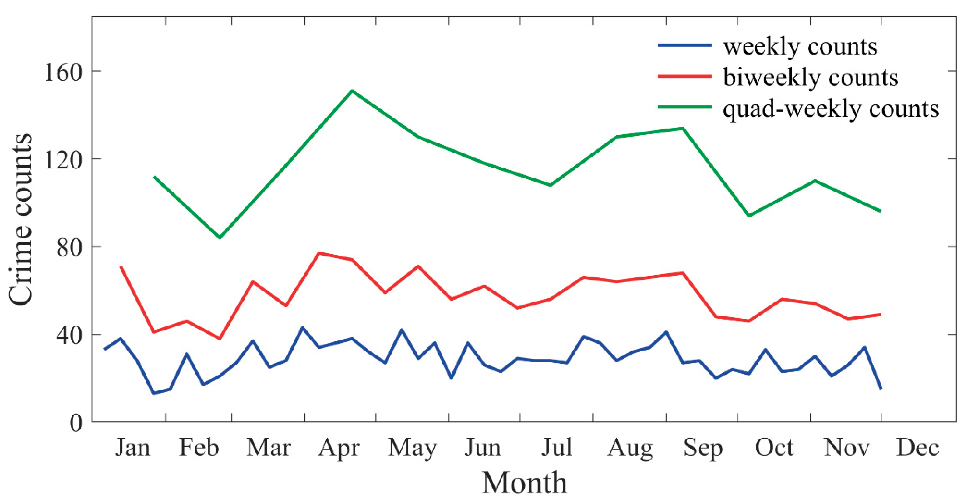
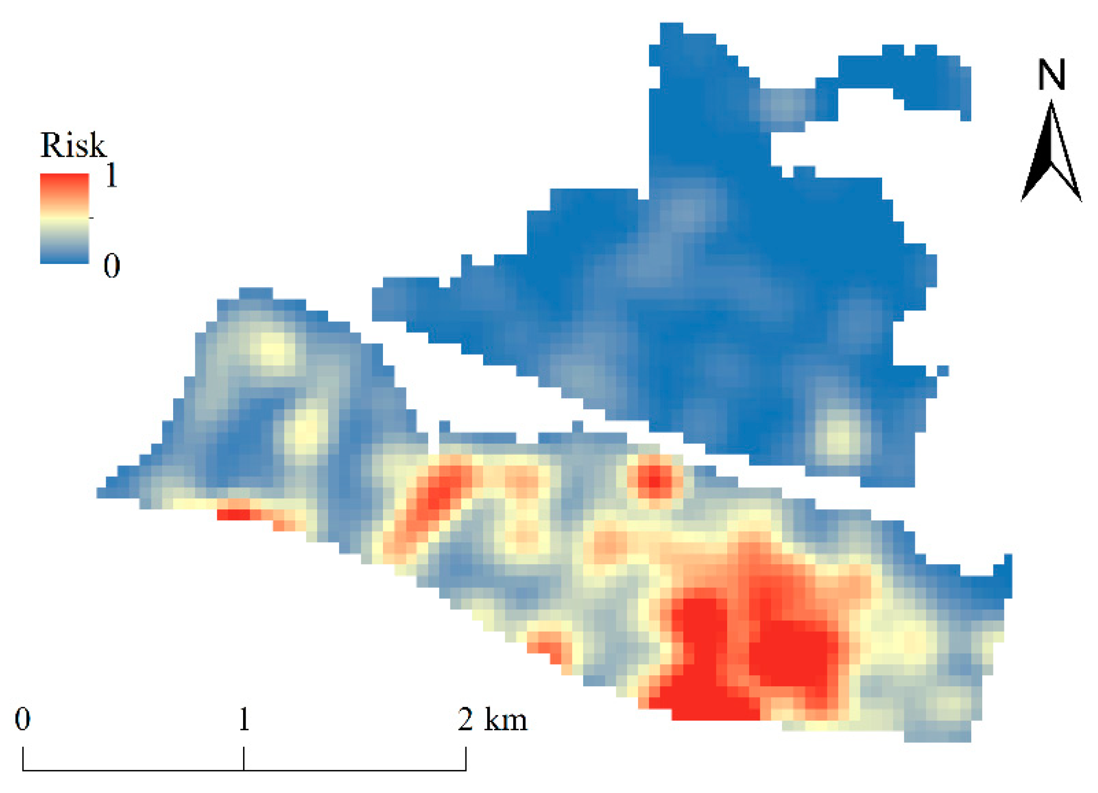
3.2.1. Historical Crime Risk (Primary Variable)

The precise historical theft and robbery data in the XT district, ZG city of China from 2 January 2017 (the first Monday of the data) to 3 December 2017 (the last Sunday of the data) are used in this study for the weekly, biweekly, and quad-weekly basis. The data from 2 January 2017 (Monday) to 5 November 2017 (Sunday) are used to calculate the historical crime risk variable (the primary variable). The data from 6 November 2017 (Monday) to 3 December 2017 (Sunday) are used for the crime prediction. We choose thefts from person and robberies from person for two reasons. (1) The vast majority of crimes in the study area fell into these two categories. There were about 3200 crime cases in the XT district from 2 January 2017 to 5 November 2017. The proportion of theft from person and robbery from person is about 55%, while those of burglary, fraud, and assault are about 8%, 7%, 9%, respectively. (2) The covariate showing the potential offenders’ activity is derived from the stop-and-question operations of the police on the street, and thefts and robberies are often considered as street crimes [36,54].

Figure 1 shows the temporal distribution of thefts and robberies for a weekly, biweekly, and quad-weekly basis. The crime counts dropped rapidly near the Spring Festival (28 January 2017). One possible reason could be that the temporary residents (mostly migrants who do not have the local Hukou) might be out of the town and visit relatives in their hometowns, so both potential offenders and victims decreased [55]. With the return of these temporary residents after the major holiday, the crime counts kept increasing until the end of April. From May to July, the crime counts dropped again because of the prolonged rainy days. People are unlikely to go outside in inclement weather, and street crime was suppressed [56,57,58]. From mid-September to early December, the crime counts were lower than the earlier stage. One of the possible explanations is that the local police department initiated proactive crime prevention strategies, which deterred the potential criminals and suppressed crime opportunities.

The primary variable, historical crime risk is built by preprocessing the theft and robbery data with kernel density estimation (KDE) [59]. We set the$Z{\left(x\right)}_k$ as the kernel density at the crime point x:

$$Z{\left(x\right)}_k={{\displaystyle \sum }}_{i=1}^n\frac{1}{nh}k\left(\frac{x-X_i}{h}\right),$$

(1)

where $h$ is the threshold value of the distance decay of $x$. $n$ is the number of crime points whose distance from $x$ is not greater than $h$. $k$ is the spatial weight function:

$$k\left(x\right)=\{\begin{array}{r}3{\pi }^{-1}(1-x^{T}x{)}^2, x^{T}x<1\\ 0, x^{T}x\ge 1\end{array},$$

(2)

The normalization of crime risk value is needed to avoid the error in prediction results caused by the inconsistency of dimensions between the primary variables and the covariate. Since the crime distribution does not follow the normal distribution [60], this study chooses the Min-Max Scaling normalization method, which can scale these data equally to the range of [0,1]:

$$Z{\left(x\right)}_n=\frac{Z{\left(x\right)}_{k }-Z{\left(x\right)}_{min}}{Z{\left(x\right)}_{max}-Z{\left(x\right)}_{min}},$$

(3)

where the $Z{\left(x\right)}_n$ is the normalized crime risk value at $x$, $Z{\left(x\right)}_{max} \mathrm{and} Z{\left(x\right)}_{min}$ are the maximum value and the minimum value respectively of the crime risk value in the whole study area. The normalized historical crime risk value (hereafter historical crime risk) is the primary variable in the crime prediction models.

Figure 2 shows the spatial distribution of the normalized historical crime risk in the XT police district. It is clear that after the normalization, the crime risk is not evenly distributed in the study area. As expected, the area at the south of the inner road experiences a much more severe crime problem than the north. The complex built and social environments in the south region result in the concentration of crime generators/attractors, which in turn promotes the convergence of potential offenders and victims. On the contrary, the relatively homogeneous land use and population composition in the north do not create many crime opportunities.

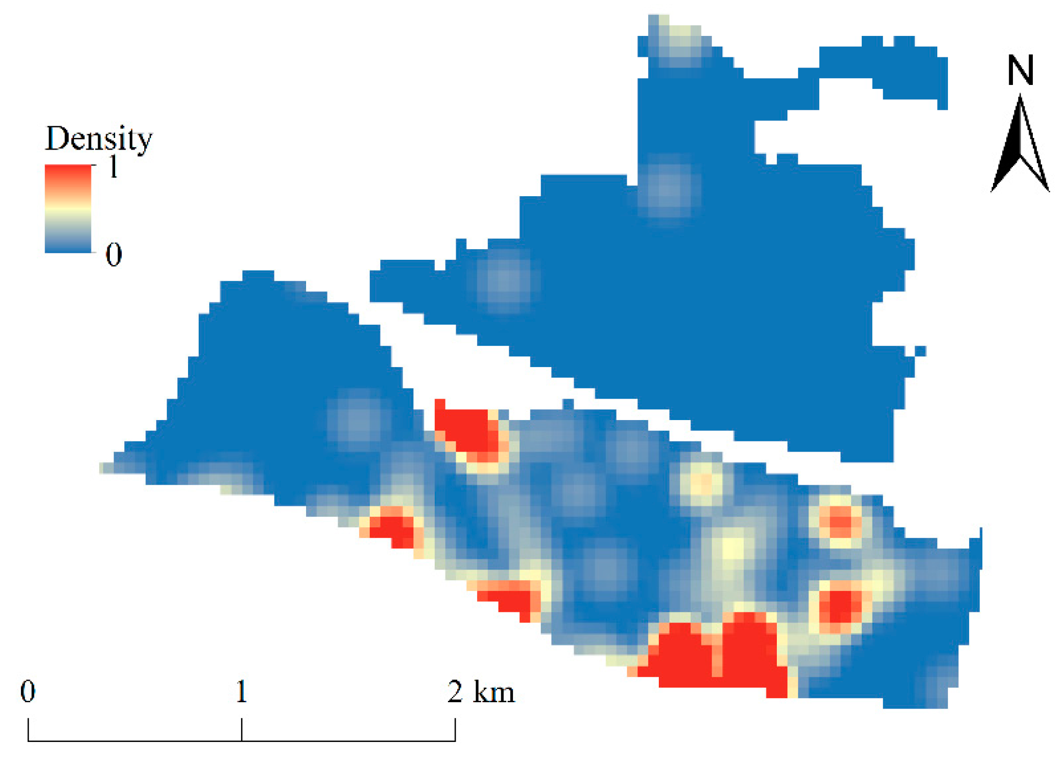
3.2.2. Potential Offenders (Covariate)

Following the general strain theory, we select the previous offenders’ activity nodes, which were derived from the stop-and-question activities of the police, as the indicator of the potential offenders. The recidivism chance of them is high, and their activity nodes usually do not change much [25,39,61,62,63]. So, the activity patterns of these previous offenders can be seen as those of the real offenders. The data from 11 September 2017 to 3 December 2017 are used to calculate the KDE of the potential offenders for a weekly, biweekly, and quad-weekly basis. They are also used to assess the correlation between potential offenders and real crime patterns. The data from 6 November 2017 to 3 December 2017 are used to build the covariate for the prediction.

The past offenders’ activity nodes are derived from the stop-and-question activities of the police. During their patrol, police officers may check the Identification Card of suspicious individuals, and every stop-and-question is recorded in the police information system. If this individual was identified as a criminal suspect or a previous offender, this record is highlighted. The precise time and location of the stop-and-question are recorded as well. Individuals who are considered as a criminal suspect or a previous offender can be classified into several groups: (1) Public disorder offenders: people who committed an offense on the social order and social stability; (2) Drug-related offenders: people who engaged in drug trafficking, drug purchasing, drug abuse, and other drug-related activities; (3) Fugitives: people who are running away or hiding to avoid being caught by the police; and (4) Other past criminals: people who served their time in prison/jail.

Similarly, the counts of the potential offenders and the percentage of them in the total people who were checked are analyzed on a weekly, biweekly, and quad-weekly basis (Figure 3). During the period from 11 September 2017 to 3 December 2017, 150 previous offenders were identified through stop-and-question. There are 81 public disorder offenders, 24 drug-related offenders, 7 fugitives, and 46 other past criminals. The general trend of both the counts and the percentage of the potential offenders peaked in the middle days of September, October, and November. Then, the counts increased significantly in early December, while the percentage was also improved slightly. The possible reason is that people begin to increase outdoor social activities toward the end of the year, and the chances of theft and robbery increase, too.

KDE is performed for the covariate after the Min-Max Scaling normalization. Figure 4 shows the spatial distribution of the potential offenders’ activity in the study area. The hot spots tend to be located near bus stations and urban villages. Such association between crime attractors and crime generators such as bus stops and urban villages and offender movement has been long established in the literature on crime pattern theory and routine activity theory [55,64]. Furthermore, this distribution is similar to that of crime hot spots in Figure 2. The similarities between the spatio-temporal distributions of the primary variable and the covariate further suggest the reasonability of using the previous offenders’ activity nodes as an alternative to locating the potential offenders’ activity nodes. Note that in the prediction models, the normalized spatial density values of the potential offenders’ activity are enlarged 10 times to enhance the influence of the covariates on the crime prediction, so the range of values is enlarged from [0,1] to [0,10] in the prediction.

3.2.3. Correlation between the Primary Variable and the Covariate

We further calculate the correlation between the historical crime risk and the potential offenders’ distribution in the same period for the weekly, biweekly, and quad-weekly basis to verify the reasonability of covariate choice. Since the period of the primary variable (historical crime risk before the prediction period) and that of the covariate (distribution of potential offenders in the prediction period) is mismatched, the correlation between the historical crime risk in one period and the potential offenders’ distribution in the following period are also tested to check their possible collinearity. Since the distributions of the two variables do not follow the normal distribution, the Spearman Rank Correlation method [65,66] is used for the correlation analysis.

Table 1. The Spearman Rank Correlation between historical crime distribution and potential offenders’ distribution.

	Historical Crime Distribution
Potential Offenders’ Distribution	Periods (in the year 2017)	09.11	09.18	09.25	10.02	10.09	10.16	10.23	10.30
	The same period (weekly)	0.096 **	0.220 **	0.059 **	0.200 **	0.256 **	0.029 **	0.097 **	0.200 **
	The following period (weekly)	0.311 **	0.283 **	0.005 **	0.197 **	0.134 **	0.085 **	0.291 **	0.161 **
	The same period (biweekly)	0.326 **		0.156 **		0.355 **		0.298 **
	The following period (biweekly)	0.261 **		0.228 **		0.147 **		0.133 **
	The same period (quad-weekly)	0.287 **				0.470 **
	The following period (quad-weekly)	0.365 **				0.374 **

Note: ** indicates a significant correlation at the 99% confidence level.

shows the Spearman Rank Correlation coefficients of the correlation between the crime distribution and the potential offenders’ distribution in the same period. The coefficients increase from 0.029 to 0.256, from 0.156 to 0.355, and from 0.287 to 0.470 for a weekly, biweekly, and quad-weekly basis, respectively. The average values are 0.145, 0.284, and 0.379 for a weekly, biweekly, and quad-weekly basis, respectively. All of these coefficients are significant under the confidence level of 0.01, indicating that the potential offender distribution holds a significant influence on the crime distribution at any temporal scales in the same period. Based on the coefficients, the correlation between the potential offender distribution and the crime distribution exists, although it is generally weak. Moreover, the coefficient increases with the expansion of the time unit from week to quad-weeks, which means the coarser time scale results in a stronger correlation.

We also test the correlation between the crime distribution in one period (taken as the primary variable) and the potential offenders’ distribution in the following period (taken as the covariate) to check their collinearity, which is also shown in Table 1. The coefficients increase from 0.005 to 0.311, from 0.133 to 0.261, and from 0.365 to 0.374 for a weekly, biweekly, and quad-weekly basis, respectively. The average values are 0.183, 0.190, and 0.370 for a weekly, biweekly, and quad-weekly basis, respectively. All of the coefficients are significant under the confidence level of 0.01, indicating that their correlation persists in the mismatched period and can be used to predict crimes. What’s more, all the coefficients are lower than 0.5, which means that the collinearity between the primary variable and the covariate is not too strong to affect the model accuracy. Similarly, the coarser time scale results in a stronger correlation, proving that the collinearities for quad-weekly basis are stronger than those for the weekly and biweekly basis.

4. Research Method: ST-Cokriging

4.1. Mathematical Principles

In this study, ST-Cokriging is used for the crime prediction. ST-Cokriging is an extension of the Cokriging system to the spatio-temporal domain [26]. Cokriging is a multivariate variant of the Kriging operation [67], which adds a secondary covariate(s) into the calculations to enhance the accuracy of predictions and solved problems of making accurate predictions of a response based on spatial interpolation [68,69,70]. Compared with other common models used in crime prediction, such as Risk Terrain modeling [71], this new ST-Cokriging algorithm can consider spatial, temporal, and spatio-temporal correlations of crime, together with a contributing variable as the covariate. Integration of the spatio-temporal trends of crime and the spatial pattern of the covariate contributes to the increased prediction accuracy.

The proposed Cokriging predictor is

$$Z\left(s_0,t_0\right)={{\displaystyle \sum }}_{i=1}^T{{\displaystyle \sum }}_{j=1}^{N_i}{\alpha }_{ij}{Z}_1\left(s_{ij},t_{1i}\right)+{{\displaystyle \sum }}_{k=1}^M{\beta }_k{Z}_2\left(s_k,t_2\right) ,$$

(4)

where $Z\left(s_0,t_0\right)$ is the predictive crime risk value at the location $x_0$ and at time $t_0$; $Z_1\left(s_{ij},t_{1i}\right)$ is the real crime risk value at the location $s_{ij}$ and at time $t_{1i}$; $Z_2\left(s_k,t_2\right)$ is the density of potential offender at the location $s_k$ and at time $t_2$. ${\alpha }_{ij}$ and ${\beta }_k$ are the weight coefficients of the primary variable and the covariate to be calculated from the linear system where $j=1,\dots ,N\_i;i=1,\dots , T;k=1,\dots , M$. Two sets of the weights ${\alpha }_{ij}$ and ${\beta }_k$ are under two constraints:

$${{\displaystyle \sum }}_{i=1}^T{{\displaystyle \sum }}_{j=1}^{N_i}{\alpha }_{ij}=1; {{\displaystyle \sum }}_{k=1}^M{\beta }_k=0.$$

(5)

These can be calculated by solving the linear system, which is optimally determined using the spatial best linear unbiased predictor.

The detailed mathematical formulation of ST-Cokriging has been stated in the previous research [26]. In this study, we use a similar framework, but more correlated data of potential offenders. The cross-covariance calculation and spatio-temporal structure have been updated according to the input of new data. Detrending of the historical crime risk data is achieved by subtracting the mean value of the previous crime risk from the crime risk in the specified period, because the ST-Cokriging needs the data to fit the Gaussian distribution and meet the secondary stationary assumption.

In this study, we use an ArcGIS Addin in Python to implement the modeling process (the version of ArcGIS is 10.4.1). This tool is available on Github (https://github.com/gis-yang/Crime-prediction). It has many functions and can be used to build the fitted models of spatial and temporal semi-variograms, generate the spatio-temporal covariance matrixes, and finally calculate the parameters ${\alpha }_{ij}$ and ${\beta }_k$ and output the value of $Z\left(s_0,t_0\right)$.

The primary variable was used as a training dataset since the historical crime data are the target activities to be predicted. We first input the historical crime data into this Crime-prediction Addin to estimate the fitting models of spatial and temporal semi-variograms. The Ordinary Least Square (OLS) fitting method is used. All of the spatial and temporal semi-variograms for the weekly, biweekly, and quad-weekly-based period can fit well the exponential model curve (Figure 5). The exponential model results are outputted as TXT format. Then, we input the text files of the spatial and temporal semi-variogram for the weekly, biweekly, and quad-weekly based period and get the spatio-temporal covariance matrixes file (also a TXT format file). Finally, we input the primary variable, the covariate and the spatio-temporal covariance matrixes file, and the ST-Cokriging model results are outputted as raster maps, too. We can get the final prediction of crime risk results after standardization and handling outliers.

The fitted models of the spatial semi-variogram are

$${\gamma }_s^{weekly}\left(h\right)=0.999\times {10}^{-2}·\left[1-\exp \left(-\frac{h}{2.6}\right)\right],$$

(6)

$${\gamma }_s^{biweekly}\left(h\right)=0.120\times {10}^{-1}·\left[1-\exp \left(-\frac{h}{2.35}\right)\right],$$

(7)

$${\gamma }_s^{quad-weekly}\left(h\right)=0.140\times {10}^{-1}·\left[1-\exp \left(-\frac{h}{2.35}\right)\right].$$

(8)

The fitted models of the temporal semi-variogram are

$${\gamma }_t^{weekly}\left(l\right)=0.889\times {10}^{-2}·\left[1-\exp \left(-\frac{l}{0.452}\right)\right]+0.220\times {10}^{-2},$$

(9)

$${\gamma }_t^{biweekly}\left(l\right)=0.796\times {10}^{-2}·\left[1-\exp \left(-\frac{l}{0.475}\right)\right]+0.163\times {10}^{-2},$$

(10)

$${\gamma }_t^{quad-weekly}\left(l\right)=0.606\times {10}^{-2}·\left[1-\exp \left(-\frac{l}{0.489}\right)\right]+0.291\times {10}^{-2},$$

(11)

where ${\gamma }_s^{weekly}$, ${\gamma }_s^{biweekly}$, and ${\gamma }_s^{quad-weekly}$ are the spatial semi-variogram models for the weekly, biweekly, and quad-weekly aggregations, respectively. ${\gamma }_t^{weekly}$, ${\gamma }_t^{biweekly}$, and ${\gamma }_t^{quad-weekly}$ are the temporal semi-variogram models for the weekly, biweekly, and quad-weekly aggregations, respectively. There is a nugget effect for the temporal semi-variogram.

4.2. Accuracy Evaluation

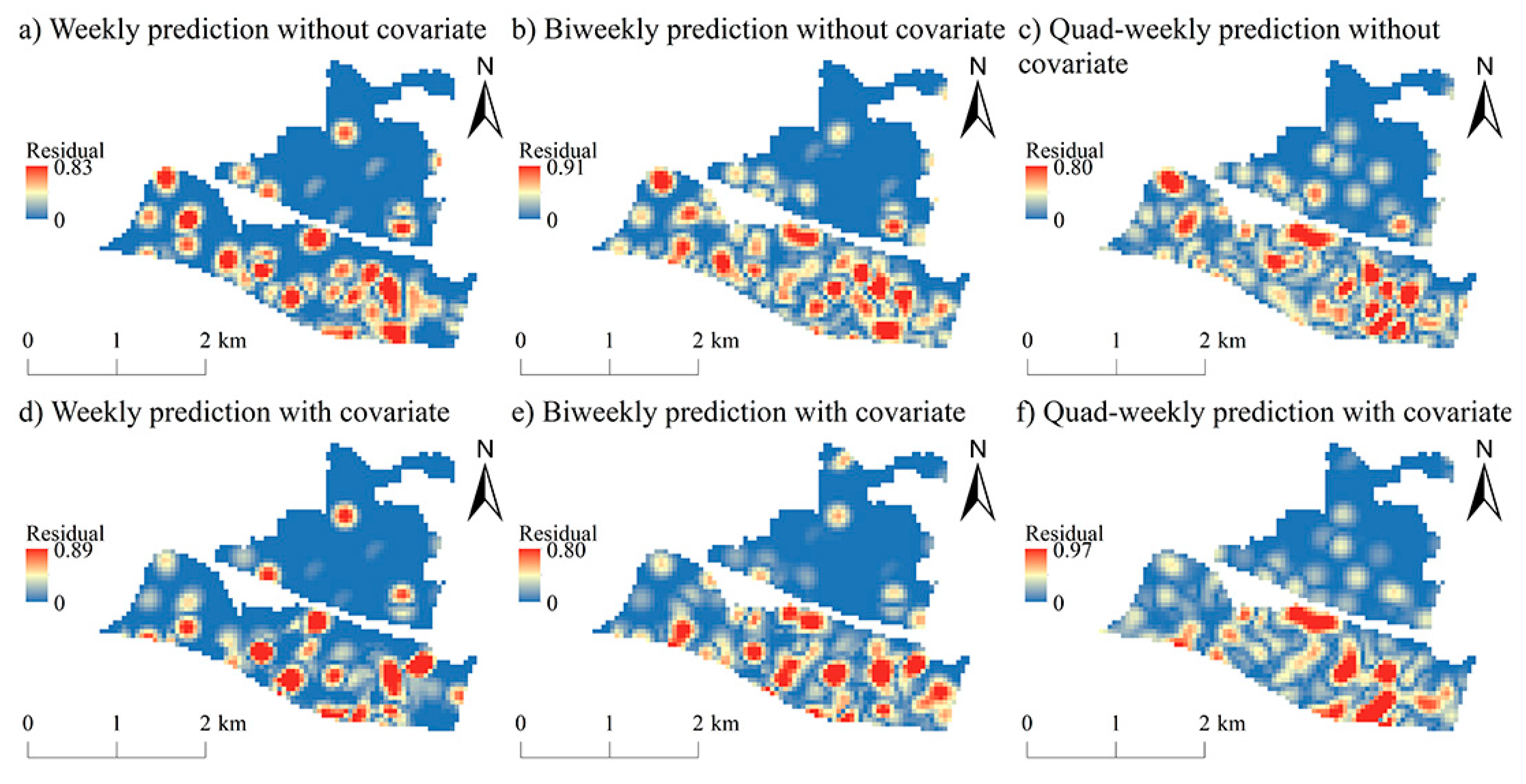
Three accuracy evaluation methods are used in the research: the Pearson Correlation Coefficient (PCC), Root Mean Squared Error (RMSE), and Predictive Accuracy Index of Raster (PAI_R). PCC and RMSE are common indicators for the measurement of the model accuracy. The formulas are as follows:

$$\mathrm{PCC}=\frac{{{\displaystyle \sum }}_{\mathrm{i}=1}^{\mathrm{n}}\left(\mathrm{Z}\left({\mathrm{x}}_{\mathrm{i}},{\mathrm{t}}_0\right)-\overline{\mathrm{Z}}\left({\mathrm{x}}_{\mathrm{i}},{\mathrm{t}}_0\right)\right)\left({\mathrm{Z}}_1\left({\mathrm{x}}_{\mathrm{i}},{\mathrm{t}}_0\right)-\overline{{\mathrm{Z}}_1}\left({\mathrm{x}}_{\mathrm{i}},{\mathrm{t}}_0\right)\right)}{\sqrt{{{\displaystyle \sum }}_{\mathrm{i}=1}^{\mathrm{n}}{\left(\mathrm{Z}\left({\mathrm{x}}_{\mathrm{i}},{\mathrm{t}}_0\right)-\overline{{\mathrm{Z}}_1}\left({\mathrm{x}}_{\mathrm{i}},{\mathrm{t}}_0\right)\right)}^2{{\displaystyle \sum }}_{\mathrm{i}=1}^{\mathrm{n}}{\left({\mathrm{Z}}_1\left({\mathrm{x}}_{\mathrm{i}},{\mathrm{t}}_0\right)-\overline{{\mathrm{Z}}_1}\left({\mathrm{x}}_{\mathrm{i}},{\mathrm{t}}_0\right)\right)}^2}},$$

(12)

$$\mathrm{RMSE}=\sqrt{\frac{1}{n}{\displaystyle \sum }_{i=1}^n{(\mathrm{Z}\left({\mathrm{x}}_{\mathrm{i}},{\mathrm{t}}_0\right)-{\mathrm{Z}}_1\left({\mathrm{x}}_{\mathrm{i}},{\mathrm{t}}_0\right))}^2},$$

(13)

where $\mathrm{Z}\left({\mathrm{x}}_{\mathrm{i}},{\mathrm{t}}_0\right)$ is the predictive crime risk value at the location ${\mathrm{x}}_{\mathrm{i}}$ at time ${\mathrm{t}}_0$, and ${\mathrm{Z}}_1\left({\mathrm{x}}_{\mathrm{i}},{\mathrm{t}}_0\right)$ is the real crime risk value at the same location and time. $\overline{\mathrm{Z}}\left({\mathrm{x}}_{\mathrm{i}},{\mathrm{t}}_0\right)$ and $\overline{{\mathrm{Z}}_1}\left({\mathrm{x}}_{\mathrm{i}},{\mathrm{t}}_0\right)$ are their average, respectively. n is the count of the grids in the study area. The higher PCC shows a higher correlation between the predictive result and reality. RMSE is the difference between the prediction value and the real crime risk value. The lower RMSE shows better prediction and smaller errors. The model with the higher PCC and the lower RMSE is with high accuracy.

The PAI_R is used to examine the prediction accuracy. Similar to the PAI (Predictive Accuracy Index) [9], PAI_R assesses the accuracy of prediction based on the proportion of predictive crime in the real hot spots. The main difference is that PAI_R uses crime risk measured in density instead of crime count to calculate the accuracy. The use of density is necessary because the spatial interpolation is a density-based approach rather than count-based.

We first sort the grids in descending order by the value of real crime risk (including the grids valued 0). Then, we choose the first b% grids (b1, b2, …, bi, …, bm) as the real crime hot spots, and the formula is as follows:

$${\mathrm{PAI}}_{{\mathrm{R}}_{\mathrm{b}}}=\frac{{{\displaystyle \sum }}_{\mathrm{i}=1}^{\mathrm{m}}\mathrm{Z}\left({\mathrm{x}}_{\mathrm{bi}},{\mathrm{t}}_0\right)}{{{\displaystyle \sum }}_{\mathrm{i}=1}^{\mathrm{n}}\mathrm{Z}\left({\mathrm{x}}_{\mathrm{i}},{\mathrm{t}}_0\right)}/\frac{{{\displaystyle \sum }}_{\mathrm{i}=1}^{\mathrm{m}}{\mathrm{Z}}_1\left({\mathrm{x}}_{\mathrm{bi}},{\mathrm{t}}_0\right)}{{{\displaystyle \sum }}_{\mathrm{i}=1}^{\mathrm{n}}{\mathrm{Z}}_1\left({\mathrm{x}}_{\mathrm{i}},{\mathrm{t}}_0\right)},$$

(14)

where the ${\mathrm{PAI}}_{{\mathrm{R}}_{\mathrm{b}}}$ shows the value of PAI_R in the first b% grids.$\mathrm{Z}\left({\mathrm{x}}_{\mathrm{bi}},{\mathrm{t}}_0\right)$ and ${\mathrm{Z}}_1\left({\mathrm{x}}_{\mathrm{bi}},{\mathrm{t}}_0\right)$ are the predictive crime risk value and the real crime risk value at the location ${\mathrm{x}}_{\mathrm{bi}}$ in the range of the first b% grids at the time ${\mathrm{t}}_0$, respectively. The PAI_R value shows the overlap ratio of the predictive crime pattern and the real crime pattern. The closer this value is to 1, the more accurate the prediction.

In order to validate the predicting performance of the ST-Cokriging system with multi-source variables, we build two sets of models; one set only uses the primary variable as the control group, and the other one uses both the primary variable and the covariate as the case group. The comparison of the PCC, RMSE, and PAI_R can tell us whether adding the covariate can improve the crime prediction accuracy as we expect and how much improvement can be achieved.

5. Results

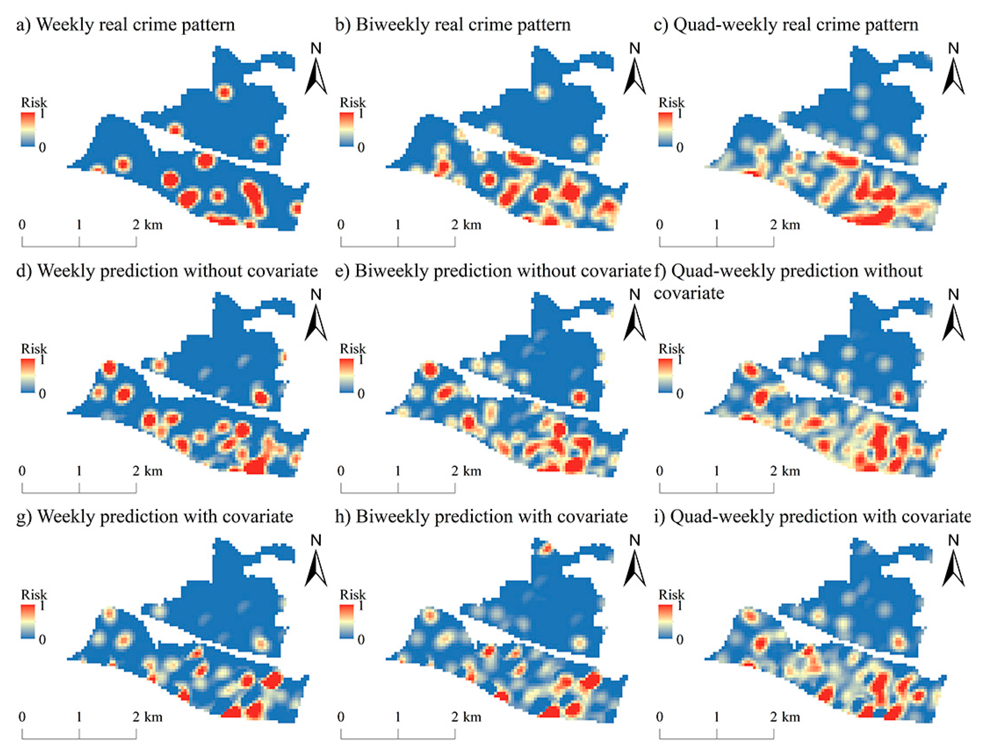
5.1. Predictive Hot Spots

We build three groups of predictive models for the weekly (6 November 2017 to 12 November 2017), biweekly (6 November 2017 to 19 November 2017), and quad-weekly (6 November 2017 to 3 December 2017) basis, respectively. Models with the covariate (the density of potential offenders) and those without the covariate are compared. All results are normalized for a better comparison.

Figure 6 shows the real crime pattern and the prediction with/without the covariate for the weekly, biweekly, and quad-weekly models. Figure 6a–c displays the real crime patterns at three different temporal scales. The crime hot spots are mainly concentrated in the southern region, and the crime concentration changes with the temporal scale change, but the hottest spots stay the same. Figure 6d–f shows the prediction results of models without the covariate, and Figure 6g–i shows the results of models with the covariate. The results of both sets of predictions (with/without the covariate) are somewhat similar to the real crime pattern with some distinctions. The prediction results of models with the covariate tend to have more precise and smaller hot spots than those without. Visual inspections show that the prediction seems to be more accurate after adding the covariate and at the coarser temporal scale.

Figure 7 shows the absolute difference between reality and prediction. Figure 7a–c displays the residual between real crime patterns and the prediction without the covariate at three different temporal scales, while Figure 7d–f displays the residual between real crime patterns and the prediction with the covariate. Clearly, fewer real crime hot spots are missed in the results of the models with the covariate. The average differences of the models without the covariate are 0.09 (weekly), 0.11 (biweekly), and 0.12 (quad-weekly). In comparison, the average differences of the models with the covariate are 0.07 (weekly), 0.08 (biweekly), and 0.10 (quad-weekly). The paired t-test (p = 0.01 < 0.05) suggests that including the covariate can significantly increase the prediction accuracy.

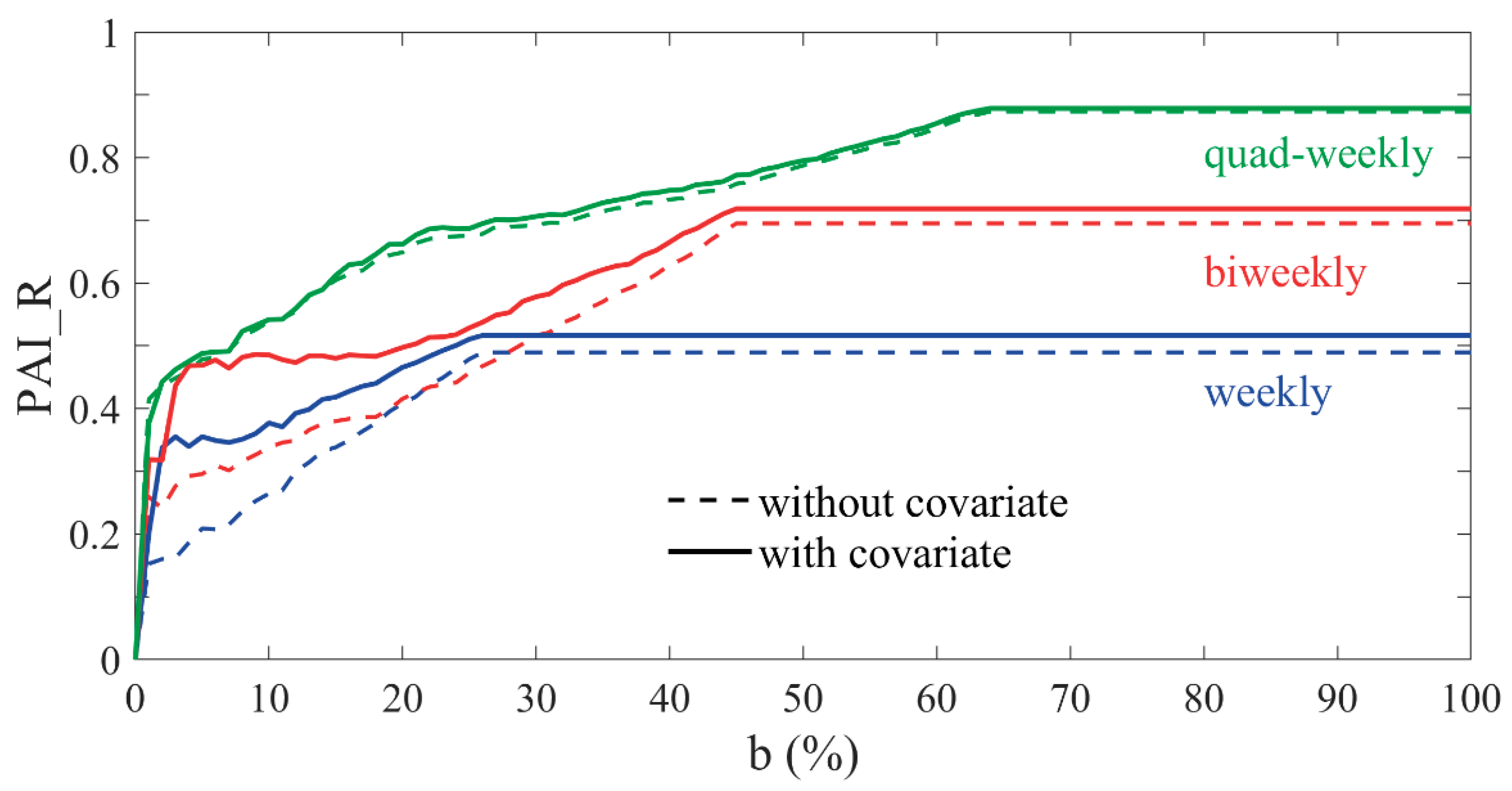
5.2. Prediction Accuracy

PCC, RMSE, and PAI_R are used to evaluate the prediction accuracy with/without the covariate (

Table 2. The Pearson Correlation Coefficient and the Root Mean Squared Error (RMSE) of the crime prediction.

Predictive Periods	Without Covariate		With Covariate
	PCC	RMSE	PCC	RMSE
6 November 2017 to 12 November 2017 (for weekly basis)	0.216 **	0.179	0.300 **	0.145
6 November 2017 to 19 November 2017 (for biweekly basis)	0.254 **	0.187	0.309 **	0.152
6 November 2017 to 3 December 2017 (for quad-weekly basis)	0.509 **	0.185	0.449 **	0.171

Note: ** indicates a significant correlation at the 99% confidence level.

). All of the PCCs are significant under the confidence level of 0.01, indicating that the predictions are highly correlated with real crime patterns. The PCCs of the models with the covariate are higher than those without the covariate in weekly (0.216 vs. 0.300) and biweekly (0.254 vs. 0.309) models except the quad-weekly models (0.509 vs. 0.449). The coefficients increase with the increase of the time-scale, indicating that data can better predict the crime over a longer period. RMSEs are also calculated for models with and without the covariate. The RMSEs of models with the covariate are lower than those without the covariate at all three time scales, indicating that the models with the covariate have significantly lower prediction errors.

Figure 8 shows the PAI_R curves for models with/without the covariate. Based on Equation (14), ${\mathrm{PAI}}_{{\mathrm{R}}_0}$ can be considered as the first value of the PAI_R curve. If b = 0, then no crime hot spot is successfully predicted in any grid of the region, so ${\mathrm{PAI}}_{{\mathrm{R}}_0}$= 0. As the area of the hot spots we defined increases, b and the corresponding ${\mathrm{PAI}}_{{\mathrm{R}}_{\mathrm{b}}}$ change accordingly. When we define all the grids where the crime risk value is not 0 (referred to as a “risky region”) as the hot spots, the corresponding b value and the corresponding PAI_R value will not change. The PAI_R curve can help us find the changing trend of the prediction accuracy with the expansion of the crime hot spots. There are almost 26% grids that can be recognized as a risky region for the weekly model, 45% for the biweekly model, and 64% for the quad-weekly model. It is obvious that the area of the risky region expands with the period increasing from one week to four weeks.

The maximum PAI_R values of the models without the covariate are 0.49 (weekly), 0.70 (biweekly), and 0.87 (quad-weekly). The maximum PAI_R values of the models with the covariate are 0.52 (weekly), 0.72 (biweekly), and 0.88 (quad-weekly). Clearly, results show that the prediction models with the covariate are consistently better than those without the covariate at any temporal resolution (paired t-test: p = 0.037 < 0.050), indicating the unneglectable contribution of the offenders’ data on crime prediction.

Additionally, the gaps are relatively large for the weekly and biweekly models but slim for quad-weekly models. The curve shows that the addition of covariate can improve the prediction accuracy in the weekly and biweekly models, but this improvement is not so obvious in the quad-weekly models. It indicates that the higher temporal resolution can significantly impact the potential offender variable on improving prediction accuracy, while the prediction with coarser temporal resolution can result in higher prediction accuracy.

6. Discussion

During the predictive periods, crime hot spots are mainly located in the southern part of the study area. There are two large urban villages and a few affordable housing complexes in the central and eastern parts of the southern region. These areas tend to breed crime because of the existence of numerous crime generators and attractors and dense street networks. Concentrated disadvantages can also help explain the theft and robbery in the lower middle class and poor neighborhoods [72]. Most people living in urban villages are rural to urban migrants who do not have urban Hukou and therefore are not entitled to many benefits enjoyed by those with urban Hukou. Over 80% of the crimes are committed by such migrant workers [55,73]. This finding is also consistent with previous studies [16,71,73]. At the same time, they can also become victims of criminal activities. It can explain the distribution of crime hot spots reasonably.

In this study, the addition of the potential offender covariate consistently improves the accuracies of the weekly, biweekly, and quad-weekly models. The results are consistent with those of recent literature on the relationship between the movement of criminals and crime patterns. Scholars reveal that crime feeds on the legal routine activities of offenders and victims and found a strong correlation between the crime and the relative mobility flow of offenders [74]. The adolescent reoffenders are more likely to commit crimes around the places they had visited or previously offended. These patterns can help forecast future crime hotspots [75]. The results also echo the previous studies about the activity of offenders and are consistent with the hypothesis that criminals often choose the familiar places around their activities as the target for the crime [21,22,23,24]. Offenders tend to act in places with abundant targets and weak safety supervision. When the attractive targets appear and the supervisory control is relaxed, it is highly possible that the potential offenders in routine activities commit crimes on the spur of the moment [2,20]. Time-sensitive offender data help capture such criminal scenario. Therefore, the addition of offender movement data can significantly improve the prediction accuracy.

We can also find that the influence of the potential offenders’ data on the crime prediction varies by different time scales. The coefficients of the PCC, RMSE, and PAI_R of predictive models are improved gradually with the expanding of a time unit from one week to four weeks, showing that the longer the time unit, the better the prediction accuracy. One of the possible reasons is the higher correlation between the activity patterns of potential offenders and the crime distribution on a larger temporal scale, which can be supported by the correlation results between the potential offenders’ pattern and the crime pattern in the same period (Table 1). The decline of time precision could increase the amount of data and eliminate some randomness, leading to a higher correlation between the potential offenders’ activity pattern and the criminal activity distribution. Therefore, the prediction accuracy in the quad-weekly group is higher than those in the weekly group and the biweekly group. It can be concluded that the lower temporal resolution of the prediction can lead to higher accuracy.

However, the contribution of the potential offenders’ data on the crime prediction is not as evident in the longer time-period prediction, when we compare the prediction results combining the covariate with those adding the primary variables only. Compared to the PAI_R curves of the models with/without the covariate in the weekly group and the biweekly group, the PAI_R curves in the quad-weekly group are more similar, which means that the improvement brought by the potential offender variable on the quad-weekly prediction is not significant than the other two groups. The possible explanation is the relatively higher correlation between the primary variable and the covariate in the models with the lower temporal resolution, which has been demonstrated in the previous analysis about the correlation between the crime distribution in one period (the primary variable) and the potential offenders’ distribution in the following period (the covariate) (Table 1). The correlation coefficients for the quad-weekly basis are much higher than those of the other groups. It may marginalize the contribution of the covariate when these two variables are added in the same models. Therefore, the addition of the potential offender variable in the quad-weekly prediction with historical crime variables at the same time may offer less improvement. The potential offender variable plays a much more critical role in predictions in shorter periods. The fact that prediction for shorter periods is far more challenging underscores the importance and contribution of the potential offender variable.

Nevertheless, there are some limitations worth exploring. The inferred movement pattern of future offenders from those of the previous offenders may not be entirely accurate (although the previous studies have demonstrated the high possibility of their recidivism). The prediction model is tested in only one city, using crime data in less than one year. These issues need to be addressed in future studies.

7. Conclusions

In this study, we applied a new ST-Cokriging crime prediction method with multi-source input data—both historical crime and temporal auxiliary data. The results revealed the effectiveness of the high temporal resolution “potential offender” covariate on the crime prediction. The results show that the accuracies of the models with the covariate are better than those without the covariate for the weekly, biweekly, and quad-weekly based periods. The new ST-Cokriging algorithm extends the spatial structure to a spatio-temporal domain; especially, the temporal independences are modeled by the temporal semi-variogram. Therefore, adding the high temporal resolution data of the potential offender into the ST-Cokriging predictive algorithm as the covariate significantly enhances the prediction accuracy than the models with historical crime data only.

Furthermore, the influence of the potential offender variable varies by the temporal resolutions of prediction. The lower the temporal prediction resolution (longer prediction period), the higher its accuracy. The reason is that the correlation between the movement of potential offenders and the crime distribution increases from the weekly period to the quad-weekly period. Nevertheless, the higher the temporal prediction resolution, the more significant the improvement of the potential offender variable on the prediction accuracy, because the prediction results in longer periods are affected by the higher collinearity between the primary variable and the covariate in the models.

This study is of significance in both academic research and professional practice. It demonstrated the complexity of the spatial and temporal distribution of criminal activities and underscored that the construction of covariates based on the classical crime theory and the fine-scale data are effective for crime prediction. Crime geography theories can guide the selection of model covariates highly related to criminal activity and improve prediction accuracy more effectively. When maintaining a certain correlation with the crime patterns, high temporal resolution data about the activity of potential offenders can avoid collinearity and offer more improvement in the short periods, which have a vital significance for the short-term crime prediction. This finding could provide insight for policing and crime prevention.

References

1. Brantingham, P.L.; Brantingham, P.J. Nodes, Paths and Edges: Considerations on the Complexity of Crime and the Physical Environment. J. Environ. Psychol. 1993, 13, 3–28. [Google Scholar] [CrossRef]
2. Kinney, J.B.; Brantingham, P.L.; Wuschke, K.; Kirk, M.G.; Brantingham, P.J. Crime attractors, generators, and detractors: Land use and urban crime opportunities. Built Environ. 2008, 34, 62–74. [Google Scholar] [CrossRef]
3. Shaw, C.R.; McKay, H.D. Juvenile Delinquency and Urban Areas; University of Chicago Press: Chicago, IL, USA, 1942. [Google Scholar]
4. Bogomolov, A.; Lepri, B.; Staiano, J.; Oliver, N.; Pianesi, F.; Pentland, A. Once upon a crime: Towards crime prediction from demographics and mobile data. In Proceedings of the 16th International Conference on Multimodal Interaction, Istanbul, Turkey, 12–16 November 2014. [Google Scholar]
5. Castelli, M.; Sormani, R.; Trujillo, L.; Popovic, A. Predicting per capita violent crimes in urban areas: An artificial intelligence approach. J. Ambient. Intell. Humaniz. Comput. 2017, 8, 29–36. [Google Scholar] [CrossRef]
6. Mohler, G.; Short, M.B.; Brantingham, P.J.; Schoenberg, F.P.; Tita, G.E. Self-Exciting point process modeling of crime. J. Am. Stat. Assoc. 2011, 106, 100–108. [Google Scholar] [CrossRef]
7. Saltos, G.; Cocea, M. An exploration of crime prediction using data mining on open data. Int. J. Inf. Technol. Decis. Mak. 2017, 16, 1155–1181. [Google Scholar] [CrossRef]
8. Wang, X.; Gerber, M.S.; Brown, D.E. Automatic crime prediction using events extracted from twitter posts. In Proceedings of the International Conference on Social Computing, Behavioral-Cultural Modeling and Prediction, Hyattsville, MD, USA, 3–5 April 2012. [Google Scholar]
9. Chainey, S.; Tompson, L.; Uhlig, S. The utility of hot spot mapping for predicting spatial patterns of crime. Secur. J. 2008, 21, 4–28. [Google Scholar] [CrossRef]
10. Eck, J.E.; Chainey, S.; Cameron, J.G.; Leitner, M.; Wilson, R.E. Mapping Crime: Understanding Hot Spots; National Institute of Justice: Washington, DC, USA, 2005.
11. Toole, J.L.; Eagle, N.; Plotkin, J.B. Spatiotemporal correlations in criminal offense records. ACM Trans. Intell. Syst. Technol. 2011, 2, 1–18. [Google Scholar] [CrossRef]
12. Kang, H.W.; Kang, H.B. Prediction of crime occurrence from multi-modal data using deep learning. PLoS ONE 2017, 12, e0176244. [Google Scholar] [CrossRef]
13. Ackerman, W.V. Socioeconomic correlates of increasing crime rates in smaller communities. Prof. Geogr. 2010, 50, 372–387. [Google Scholar] [CrossRef]
14. Andresen, M.A. A spatial analysis of crime in Vancouver, British Columbia: A synthesis of social disorganization and routine activity theory. Can. Geographer. 2006, 50, 487–502. [Google Scholar] [CrossRef]
15. Bowers, K. Risky facilities: Crime radiators or crime absorbers? A comparison of internal and external levels of theft. J. Quant. Criminol. 2014, 30, 389–414. [Google Scholar] [CrossRef]
16. Groff, E.R.; Lockwood, B. Criminogenic facilities and crime across street segments in Philadelphia: Uncovering evidence about the spatial extent of facility influence. J. Res. Crime Delinq. 2014, 51, 277–314. [Google Scholar] [CrossRef]
17. Curtis, J.W. Integrating sketch maps with gis to explore fear of crime in the urban environment: A review of the past and prospects for the future. Am. Cartographer. 2012, 39, 175–186. [Google Scholar] [CrossRef]
18. Jií, P.; Ivan, I.; Lucie, M. Comparing Residents’ Fear of Crime with Recorded Crime Data-Case Study of Ostrava, Czech Republic. ISPRS Int. Geo-Inf. 2019, 8, 401. [Google Scholar]
19. Prieto, C.R.; Bishop, S.R. Fear of crime: The impact of different distributions of victimisation. Palgrave Commun. 2018, 4, 1–8. [Google Scholar]
20. Cohen, L.E.; Felson, M. Social change and crime rate trends: A routine activity approach. Am. Sociol. Rev. 1979, 44, 588–608. [Google Scholar] [CrossRef]
21. Bernasco, W.; Kooistra, T. Effects of residential history on commercial robbers’ crime location choices. Eur. J. Criminol. 2010, 7, 251–265. [Google Scholar] [CrossRef] [Green Version]
22. Johnson, S.D.; Bowers, K.J. Permeability and burglary risk: Are cul-de-sacs safer? J. Quant. Criminol. 2010, 26, 89–111. [Google Scholar] [CrossRef]
23. Lammers, M.; Menting, B.; Ruiter, S.; Bernasco, W. Biting once, twice: The influence of prior on subsequent crime location choice. Criminology 2015, 53, 309–329. [Google Scholar] [CrossRef]
24. Menting, B.; Lammers, M.; Ruiter, S.; Bernasco, W. Family matters: Effects of family members’ residential areas on crime location choice. Criminology 2016, 54, 413–433. [Google Scholar] [CrossRef]
25. Ackerman, A.R.; Sacks, M. Can general strain theory be used to explain recidivism among registered sex offenders? J. Crim. Justice 2012, 40, 187–193. [Google Scholar] [CrossRef]
26. Yang, B.; Liu, L.; Lan, M.; Wang, Z.; Zhou, H.; Yu, H. A spatio-temporal Cokriging method for crime prediction using historical crime data and transitional zones identified from nightlight imagery. Int. J. Geogr. Inf. Sci. 2020, 34, 1740–1764. [Google Scholar] [CrossRef]
27. Short, M.B.; D’Orsogna, M.R.; Pasour, V.B.; Tita, G.E.; Brantingham, P.J.; Bertozzi, A.L.; Chayes, L.B. A statistical model of criminal behavior. Math. Models Methods Appl. Sci. 2008, 18, 1249–1267. [Google Scholar] [CrossRef]
28. Couckuyt, I.; Koziel, S.; Dhaene, T. Surrogate modeling of microwave structures using kriging, co-kriging, and space mapping. Int. J. Numer. Model Electron. Netw. Device Fields 2013, 26, 64–73. [Google Scholar] [CrossRef]
29. Kanankege, K.S.T.; Alkhamis, M.A.; Phelps, N.B.D.; Perez, A.M. A probability co-kriging model to account for reporting bias and recognize areas at high risk for zebra mussels and Eurasian watermilfoil invasions in Minnesota. Front. Vet. Sci. 2017, 4, 231. [Google Scholar] [CrossRef] [PubMed] [Green Version]
30. Liang, X.; Schilling, K.E.; Zhang, Y.; Jones, C.S. Co-Kriging estimation of Nitrate-Nitrogen loads in an agricultural river. Water Resour. Manag. 2016, 30, 1771–1784. [Google Scholar] [CrossRef]
31. Eom, J.K.; Park, M.S.; Heo, T.; Huntsinger, L.F. Improving the prediction of annual average daily traffic for nonfreeway facilities by applying a spatial statistical method. Transp. Res. Record. 2006, 1968, 20–29. [Google Scholar] [CrossRef]
32. Zou, H.; Yue, Y.; Li, Q.; Yeh, A.G. An improved distance metric for the interpolation of link-based traffic data using kriging: A case study of a large-scale urban road network. Int. J. Geogr. Inf. Sci. 2012, 26, 667–699. [Google Scholar] [CrossRef]
33. Snepvangers, J.J.; Heuvelink, G.B.; Huisman, J.A. Soil water content interpolation using spatio-temporal kriging with external drift. Geoderma 2003, 112, 253–271. [Google Scholar] [CrossRef]
34. Sideris, I.V.; Gabella, M.; Erdin, R.; Germann, U. Real-time radar-rain-gauge merging using spatio-temporal co-kriging with external drift in the alpine terrain of Switzerland. Q. J. R. Meteorol. Soc. 2014, 140, 1097–1111. [Google Scholar] [CrossRef]
35. Bae, B.; Kim, H.; Lim, H.; Liu, Y.; Han, L.D.; Freeze, P.B. Missing data imputation for traffic flow speed using spatio-temporal cokriging. Transp. Res. Part C Emerg. Technol. 2018, 88, 124–139. [Google Scholar] [CrossRef]
36. Lan, M.; Liu, L.; Hernandez, A.; Liu, W.; Zhou, H.; Wang, Z. The Spillover Effect of Geotagged Tweets as a Measure of Ambient Population for Theft Crime. Sustainability 2019, 11, 6748. [Google Scholar] [CrossRef] [Green Version]
37. Gerber, M.S. Predicting crime using Twitter and kernel density estimation. Decis. Support Syst. 2014, 61, 115–125. [Google Scholar] [CrossRef]
38. Chen, X.; Cho, Y.; Jang, S.Y. Crime prediction using Twitter sentiment and weather. In Proceedings of the 2015 Systems and Information Engineering Design Symposium, Charlottesville, VA, USA, 24 April 2015. [Google Scholar]
39. Agnew, R. Foundation for a general strain theory of crime and delinquency. Criminology 1992, 30, 47–87. [Google Scholar] [CrossRef]
40. Fisher, B.S.; Wilkes, A.R. A tale of two ivory towers. A comparative analysis of victimization rates and risks between university students in the United States and England. Br. J. Criminol. 2003, 43, 526–545. [Google Scholar] [CrossRef]
41. Rountree, P.W.; Land, K.C. The generalizability of multilevel models of burglary victimization: A cross-city comparison. Soc. Sci. Res. 2000, 29, 284–305. [Google Scholar] [CrossRef]
42. Tseloni, A.; Wittebrood, K.; Farrell, G.; Pease, K. Burglary victimization in England and wales, the United States and the Netherlands: A cross-national comparative test of routine activities and lifestyle theories. Br. J. Criminol. 2004, 44, 66–91. [Google Scholar] [CrossRef]
43. Clarke, R.V.; Eck, J. Become a Problem-Solving Crime Analyst; Willan Publishing: Uffculme, UK, 2003. [Google Scholar]
44. Beauregard, E.; Rossmo, D.K.; Proulx, J. A descriptive model of the hunting process of serial sex offenders: A rational choice perspective. J. Fam. Violence 2007, 22, 449–463. [Google Scholar] [CrossRef]
45. Mogavero, M.C.; Hsu, K. Sex offender mobility: An application of crime pattern theory among child sex offenders. Sex. Abus. J. Res. Treat. 2018, 30, 908–931. [Google Scholar] [CrossRef]
46. Santtila, P.; Hakkanen, H.; Canter, D.V.; Elfgren, T. Classifying homicide offenders and predicting their characteristics from crime scene behavior. Scand. J. Psychol. 2003, 44, 107–118. [Google Scholar] [CrossRef]
47. Mccuish, E.C.; Cale, J.; Corrado, R.R. A prospective study of offending patterns of youth homicide offenders into adulthood. Youth Violence Juv. Justice 2018, 16, 18–36. [Google Scholar] [CrossRef]
48. Ratcliffe, J.H. A temporal constraint theory to explain opportunity-based spatial offending patterns. J. Res. Crime Delinq. 2006, 43, 261–291. [Google Scholar] [CrossRef]
49. Bernasco, W.; Nieuwbeerta, P. How do residential burglars select target areas? A new approach to the analysis of criminal location choice. Br. J. Criminol. 2005, 45, 296–315. [Google Scholar] [CrossRef] [Green Version]
50. Townsley, M.; Sidebottom, A. All offenders are equal, but some are more equal than others: Variation in journeys to crime between offenders. Criminology 2010, 48, 897–917. [Google Scholar] [CrossRef]
51. Bernasco, W. A sentimental journey to crime: Effects of residential history on crime location choice. Criminology 2010, 48, 389–416. [Google Scholar] [CrossRef]
52. Rossmo, D.K.; Lu, Y.; Fang, T.B. Spatial-temporal crime paths. In Patterns, Prevention and Geometry of Crime; Andresen, M.A., Kinney, J.B., Eds.; Routledge: New York, NY, USA, 2012; pp. 16–42. [Google Scholar]
53. Walsh, W.F. Compstat: An analysis of an emerging police managerial paradigm. Polic. Int J Police Strateg. Manag. 2001, 24, 347–362. [Google Scholar] [CrossRef]
54. Rosenfeld, R.; Fornango, R. The impact of economic conditions on robbery and property crime: The role of consumer sentiment. Criminology 2007, 45, 735–769. [Google Scholar] [CrossRef]
55. Liu, L.; Feng, J.; Ren, F.; Xiao, L. Examining the relationship between neighborhood environment and residential locations of juvenile and adult migrant burglars in China. Cities 2018, 82, 10–18. [Google Scholar] [CrossRef]
56. Blakeslee, D.S.; Fishman, R. Weather shocks, agriculture, and crime: Evidence from India. J. Hum. Resour. 2018, 53, 750–782. [Google Scholar] [CrossRef]
57. Horrocks, J.; Menclova, A.K. The effects of weather on crime. N. Z. Econ. Pap. 2011, 45, 231–254. [Google Scholar] [CrossRef]
58. Linning, S.J.; Andresen, M.A.; Brantingham, P.J. Crime seasonality: Examining the temporal fluctuations of property crime in cities with varying climates. Int. J. Offender Ther. Comp. Criminol. 2016, 61, 1866–1891. [Google Scholar] [CrossRef] [PubMed]
59. Silverman, B.W. Density Estimation for Statistics and Data Analysis; Chapman and Hall: London, UK, 1987. [Google Scholar]
60. Wilcox, P.; Eck, J.E. Criminology of the unpopular: Implications for policy aimed at payday lending facilities. Criminol. Public Policy 2011, 10, 473–482. [Google Scholar] [CrossRef]
61. Banse, R.; Koppehelegossel, J.; Kistemaker, L.M.; Werner, V.A.; Schmidt, A. Pro-criminal attitudes, intervention, and recidivism. Aggress. Violent Behav. 2013, 18, 673–685. [Google Scholar] [CrossRef] [Green Version]
62. Braverman, D.W.; Doernberg, S.N.; Runge, C.P.; Howard, D.S. OxRec model for assessing risk of recidivism: Ethics. Lancet Psychiatry 2016, 3, 808–809. [Google Scholar] [CrossRef] [Green Version]
63. Fazel, S.; Chang, Z.; Fanshawe, T.R.; Langstrom, N.; Lichtenstein, P.; Larsson, H.; Mallett, S. Prediction of violent reoffending on release from prison: Derivation and external validation of a scalable tool. Lancet Psychiatry 2016, 3, 535–543. [Google Scholar] [CrossRef] [Green Version]
64. Liu, L.; Lan, M.; Eck, J.E.; Kang, E.L. Assessing the effects of bus stop relocation on street robbery. Comput. Environ. Urban 2020, 80, 101455. [Google Scholar] [CrossRef]
65. Gauthier, T.D. Detecting trends on using Spearman’s rank correlation co-efficient. Enviorn. Forensic 2001, 2, 359–362. [Google Scholar] [CrossRef]
66. Selinger, C.P.; Ochieng, A.O.; George, V.; Leong, R.W. The accuracy of adherence self-report scales in patients on thiopurines for inflammatory bowel disease: A comparison with drug metabolite levels and medication possession ratios. Inflamm. Bowel Dis. 2019, 25, 919–924. [Google Scholar] [CrossRef]
67. Krige, D.G. A Statistical Approach to Some Mine Valuations and Allied Problems at the Witwatersrand. Master’s Thesis, The University of Witwatersrand, Johannesburg, South Africa, 1951. [Google Scholar]
68. Atkinson, P.M.; Pardoiguzquiza, E.; Chicaolmo, M. Downscaling Cokriging for super-resolution mapping of continua in remotely sensed images. IEEE Trans. Geosci. Remote Sens. 2008, 46, 573–580. [Google Scholar] [CrossRef]
69. Chilès, J.; Delfiner, P. Geostatistics: Modeling Spatial Uncertainty; Wiley: New York, NY, USA, 1999. [Google Scholar]
70. Cressie, N.A.C. Statistics for Spatial Data; Wiley: New York, NY, USA, 1993. [Google Scholar]
71. Joel, M.C.; Leslie, W.K.; Miller, J. Risk terrain modeling: Brokering criminological theory and GIS methods for crime forecasting. Justice Q. 2011, 28, 360–381. [Google Scholar]
72. Melo, S.N.; Pereira, D.V.; Andresen, M.A.; Matias, L.F. Spatial/temporal variations of crime: A routine activity theory perspective. Int. J. Offender Ther. Comp. Criminol. 2018, 62, 1967–1991. [Google Scholar] [CrossRef] [PubMed]
73. Wang, Z. Crime Research in Three Big Economy Regions in Contemporary China; China People’s Public Security University Press: Beijing, China, 2006. [Google Scholar]
74. Song, G.; Bernasco, W.; Liu, L.; Xiao, L.; Zhou, S.; Liao, W. Crime feeds on legal activities: Daily mobility flows help to explain thieves’ target location choices. J. Quant. Criminol. 2019, 35, 831–854. [Google Scholar] [CrossRef] [Green Version]
75. Bernasco, W. Adolescent offenders’ current whereabouts predict locations of their future crimes. PLoS ONE 2019, 14, e0210733. [Google Scholar] [CrossRef] [PubMed]
Figure 1. The temporal distribution of weekly, biweekly, and quad-weekly crime counts in the XT police district (2 January 2017 to 3 December 2017).
Ijgi 09 00732 g001
Figure 2. The spatial distribution of the historical crime risk in the XT police district (2 January 2017 to 3 December 2017).
Ijgi 09 00732 g002
Figure 3. The temporal distribution of the potential offenders in the XT police district on a weekly, biweekly, and quad-weekly basis (11 September 2017 to 3 December 2017).
Ijgi 09 00732 g003
Figure 4. The spatial distribution of the potential offenders in the XT police district (11 September 2017 to 3 December 2017).
Ijgi 09 00732 g004
Figure 5. The spatial semi-variogram (a,c,e), temporal semi-variogram (b,d,f), and fitting models of the primary variable.
Ijgi 09 00732 g005
Figure 6. The real crime pattern (ac), the predictive results without the covariate (df), and the predictive results with the covariate (gi) for the weekly, biweekly, and quad-weekly basis.
Ijgi 09 00732 g006
Figure 7. The absolute differences between the predictions and the reality ((ac), prediction without the covariate; (df), prediction with the covariate).
Ijgi 09 00732 g007
Figure 8. The Predictive Accuracy Index of Raster (PAIR) curves for the weekly, biweekly, and quad-weekly models.
Ijgi 09 00732 g008