Combining Satellite Remote Sensing and Climate Data in Species Distribution Models to Improve the Conservation of Iberian White Oaks (Quercus L.)

Abstract

The Iberian Peninsula hosts a high diversity of oak species, being a hot-spot for the conservation of European White Oaks (Quercus) due to their environmental heterogeneity and its critical role as a phylogeographic refugium. Identifying and ranking the drivers that shape the distribution of White Oaks in Iberia requires that environmental variables operating at distinct scales are considered. These include climate, but also ecosystem functioning attributes (EFAs) related to energy–matter exchanges that characterize land cover types under various environmental settings, at finer scales. Here, we used satellite-based EFAs and climate variables in species distribution models (SDMs) to assess how variables related to ecosystem functioning improve our understanding of current distributions and the identification of suitable areas for White Oak species in Iberia. We developed consensus ensemble SDMs targeting a set of thirteen oaks, including both narrow endemic and widespread taxa. Models combining EFAs and climate variables obtained a higher performance and predictive ability (true-skill statistic (TSS): 0.88, sensitivity: 99.6, specificity: 96.3), in comparison to the climate-only models (TSS: 0.86, sens.: 96.1, spec.: 90.3) and EFA-only models (TSS: 0.73, sens.: 91.2, spec.: 82.1). Overall, narrow endemic species obtained higher predictive performance using combined models (TSS: 0.96, sens.: 99.6, spec.: 96.3) in comparison to widespread oaks (TSS: 0.80, sens.: 92.6, spec.: 87.7). The Iberian White Oaks show a high dependence on precipitation and the inter-quartile range of Normalized Difference Water Index (NDWI) (i.e., seasonal water availability) which appears to be the most important EFA variable. Spatial projections of climate–EFA combined models contribute to identify the major diversity hotspots for White Oaks in Iberia, holding higher values of cumulative habitat suitability and species richness. We discuss the implications of these findings for guiding the long-term conservation of Iberian White Oaks and provide spatially explicit geospatial information about each oak species (or set of species) relevant for developing biogeographic conservation frameworks.

1. Introduction

The genus Quercus L. is one of the most abundant and economically important group of woody plants in the Northern Hemisphere [1], and oak forests are the keystone species in many Mediterranean and Temperate forests and woodlands, providing fundamental regulation, provision, support and cultural ecosystem services for people and nature [2,3,4,5,6]. The Iberian Peninsula (IP) harbours half of the European diversity of oak species, when excluding intraspecific variation [7,8,9,10]. The IP is a major glacial refugia [11] and a major hotspot for the White Oaks group (Sect. Quercus) [12] partly due to its paleoclimatic history and the presence of two major biogeographic regions (Eurosiberian and Mediterranean). The ecotone between these two biogeographic regions is widely occupied by marcescent forests dominated by White Oaks either deciduous or marcescent spanning across the sub-Mediterranean belt [13,14,15,16]. Climate change seriously threatens these transition zones, as summer periods become increasingly arid and warm in the coming decades [6,17]. Additionally, land use/cover changes, forest management practices that favour fast growing tree species (e.g., Eucalyptus spp.), and invasive species along with wildfires and other disturbances [18,19] also pose serious threats to these already marginal and fragile ecosystems in the IP.

Traditionally, seven White Oak species are considered to be native to the IP, when excluding infraspecific variation [7]. However, the known low interspecific barriers to gene flow give this genus a complex evolutionary and speciation pattern, which includes the formation of new species as a result of hybridization (i.e., nothotaxa) [20,21]. Previous studies refer to cryptic taxa that are notable in the IP [9,22,23,24,25,26], including narrow distributed and endemic (NDE) species or relict taxa [27,28,29]. This confers to the Iberian White Oak forests with high phylogeographic value in addition to the value for human well-being and especially relevance for mitigating climate-driven risks [2,3].

Given their eco-evolutionary importance, White Oak species and related ecosystems require suitable geospatial analysis tools to assess their conservation status and demographic trends [30]. In this regard, species distribution models (hereafter SDMs, i.e., habitat suitability models or ecological niche models) are among the most widely used tools to assess the impact of global change on biodiversity, and to inform policy makers [31]. In a nutshell, SDMs allow to understand species–environment relations by modelling between the occurrence or abundance of species and environmental predictors (e.g., temperature, rainfall, soil type, vegetation cover) that determine it. This is done through empirical/correlative and mainly static approaches, based on statistical or machine learning algorithms which use as input species field observations, and/or museum-type records. The obtained species–environment responses are thought to best reflect the realized ecological niche of the study species [32]. Trained models are used to obtain spatiotemporal projections of species distributions based on current, past or future conditions to gain insights on the environmental drivers that shape the potential (or actual) occurrence of study species at multiple spatial scales.

Complementarily to innovative SDM approaches, recent advances in satellite remote sensing (SRS), with the ever increasing availability of data with enhanced spatial and spectral features, allow us to continuously depict Earth system dynamics in its multiple facets relevant for species and biodiversity monitoring [33]. These are capable of capturing the intra-annual dynamics of ecosystem functioning such as the average annual conditions, intra-annual seasonal variation, phenology or extreme values for several relevant dimensions. In particular, satellite-based ecosystem functioning attributes (EFAs) [34,35] defined as spatiotemporal integrative descriptors of ecosystem functioning and dynamics computed from time series of satellite products (e.g., spectral indices for vegetation or water) are providing new opportunities to push the boundaries of SDMs. EFAs inform on several relevant features of ecosystem functioning such as primary productivity, evapotranspiration, land surface temperature, and albedo, thereby encompassing several dimensions including carbon gains, water and energy balance [36,37,38]. EFAs are considered essential biodiversity variables (EBVs) describing the ‘Ecosystem Function’ class [39]. Therefore, the EFA framework provides key variables to model the ecosystem processes that maintain suitable environmental and habitat conditions for keystone species [40,41]. This will allow us to anticipate species’ range shifts under global change [30]. Overall, EFAs offer an alternative and cost-effective approach to improve predictions on the distribution of species and support biodiversity monitoring once these are capable of capturing the intra-annual dynamics of ecosystem functioning.

Although the use of SDMs has played a major role in oak forest conservation [42,43], they have been mainly applied to iconic oak species, like cork oak (Q. suber L.) [44,45], or to broadly distributed species (e.g., Q. robur) or species groups [46,47], sometimes at smaller and regional scales [48,49]. We lack to date studies encompassing narrow distributed and endemic (NDE), relict species, especially in a phylogeographic hotspot such as the IP. This knowledge gap mainly derives from issues related to the taxonomic uncertainty and delimitation of species, which in turn hampers data quality and quantity. These data are typically based on inflated nomenclatural inaccuracy and outdated, due to misleading identification that results from ancient herbaria reviews. Still, it is the biggest bulk of information available in worldwide databases (e.g., https://www.gbif.org/), but its limitations hinder the process of accurately predicting species distributions across geographic space, hampering conservation efforts [50,51,52]. Furthermore, previous modelling techniques mostly rely on climatic envelopes that perform better at broad global scales, and they tend to overlook ecosystem functioning features at a fine spatial scale. To overcome this situation, SRS-based ecosystem functioning attributes integrate the effects of vegetation structure, edaphic conditions and climate at the fine local/meso scale. This makes these variables suitable to improve predictions regarding species optimal environmental conditions, to forecast the effects of environmental change, to monitor biodiversity hotspots, or to model habitat quality from local/regional to global scales [37,40,41].

This study aimed to assess whether the combination of EFA and climate variables improves the performance of SDMs using seven narrow distributed or endemic Iberian White Oaks: Quercus canariensis, Q. ×cerrioides, Q. estremadurensis, Q. lusitanica, Q. marianica, Q. orocantabrica and Q. subpyrenaica along with six widespread species Q. broteroi, Q. faginea, Q. pyrenaica, Q. petraea, Q. pubescens and Q. robur. For this aim, we developed a set of combined models (integrating EFA and climate variables) and partial models (either EFA or climate variables). We compared their performance through several metrics and identified the most suitable areas to preserve threatened species. With this goal in mind, we specifically:

(i)

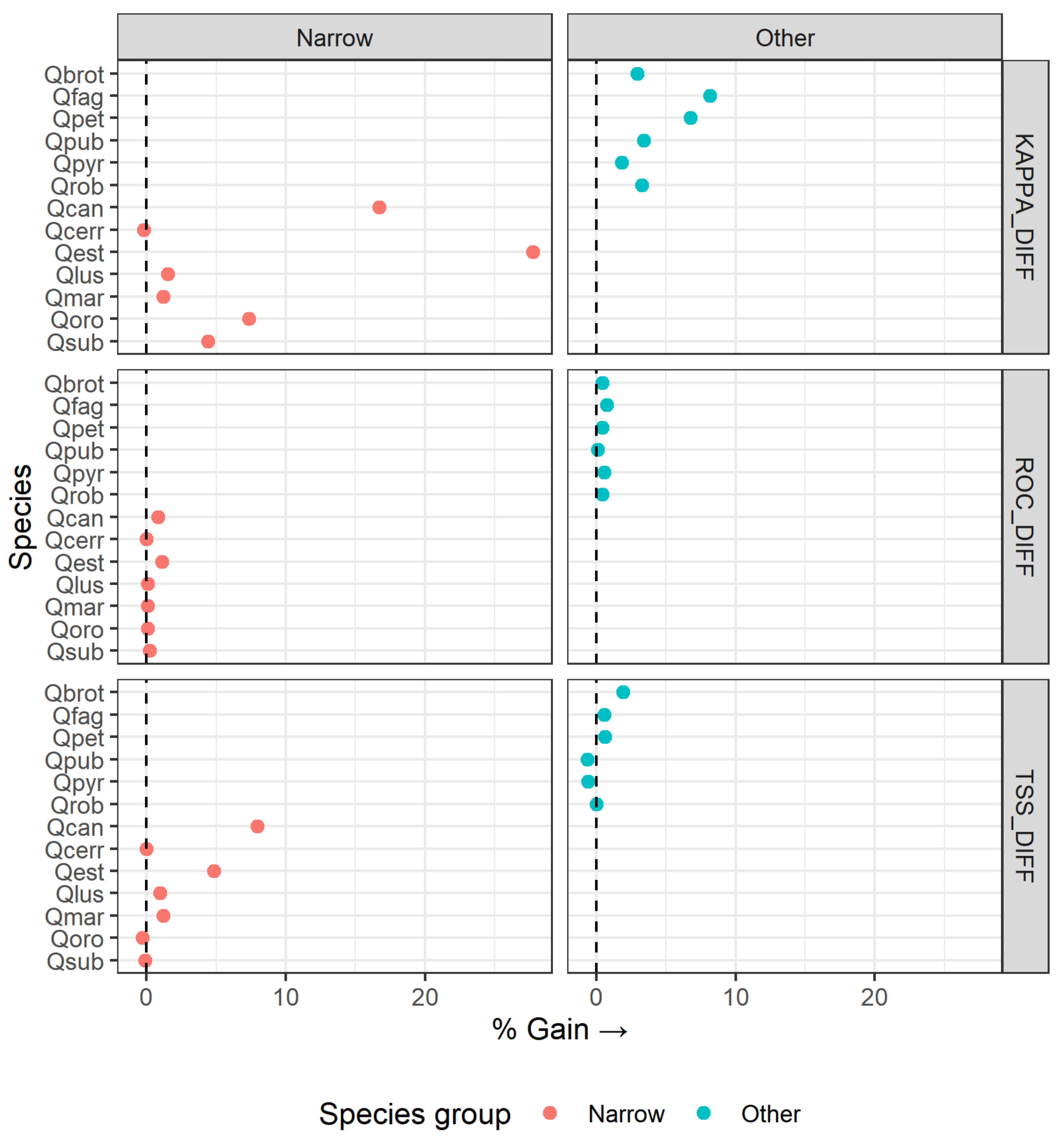
Compared the performance of SRS-EFAs as predictors in SDMs, separately and combined with climate data, to determine the current potential distribution of the thirteen target species;

(ii)

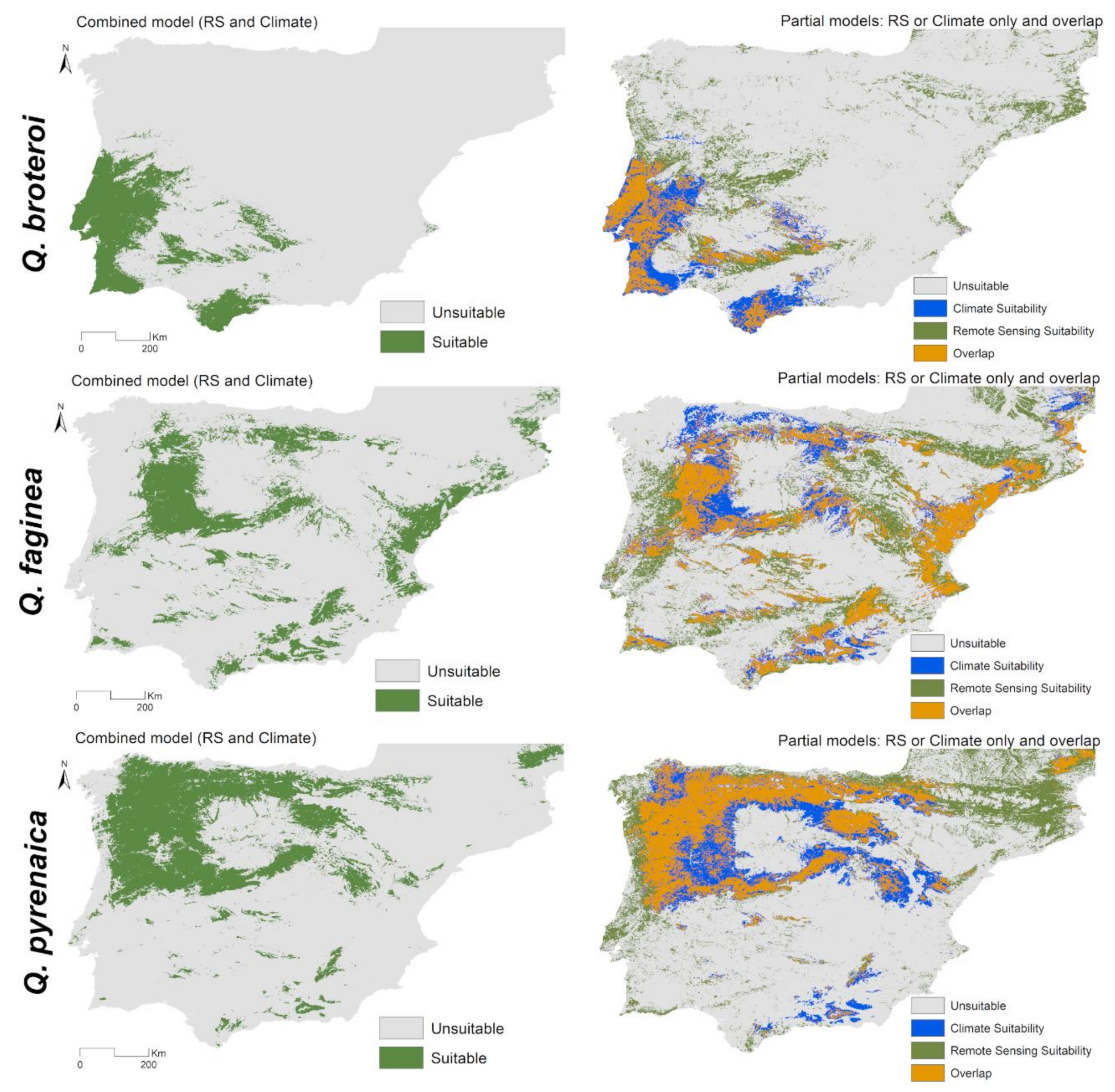
Identified the most suitable potential areas for the conservation of vulnerable NDE oak species by comparing the spatial projections of habitat suitability derived from SDMs based on different sets of predictors;

(iii)

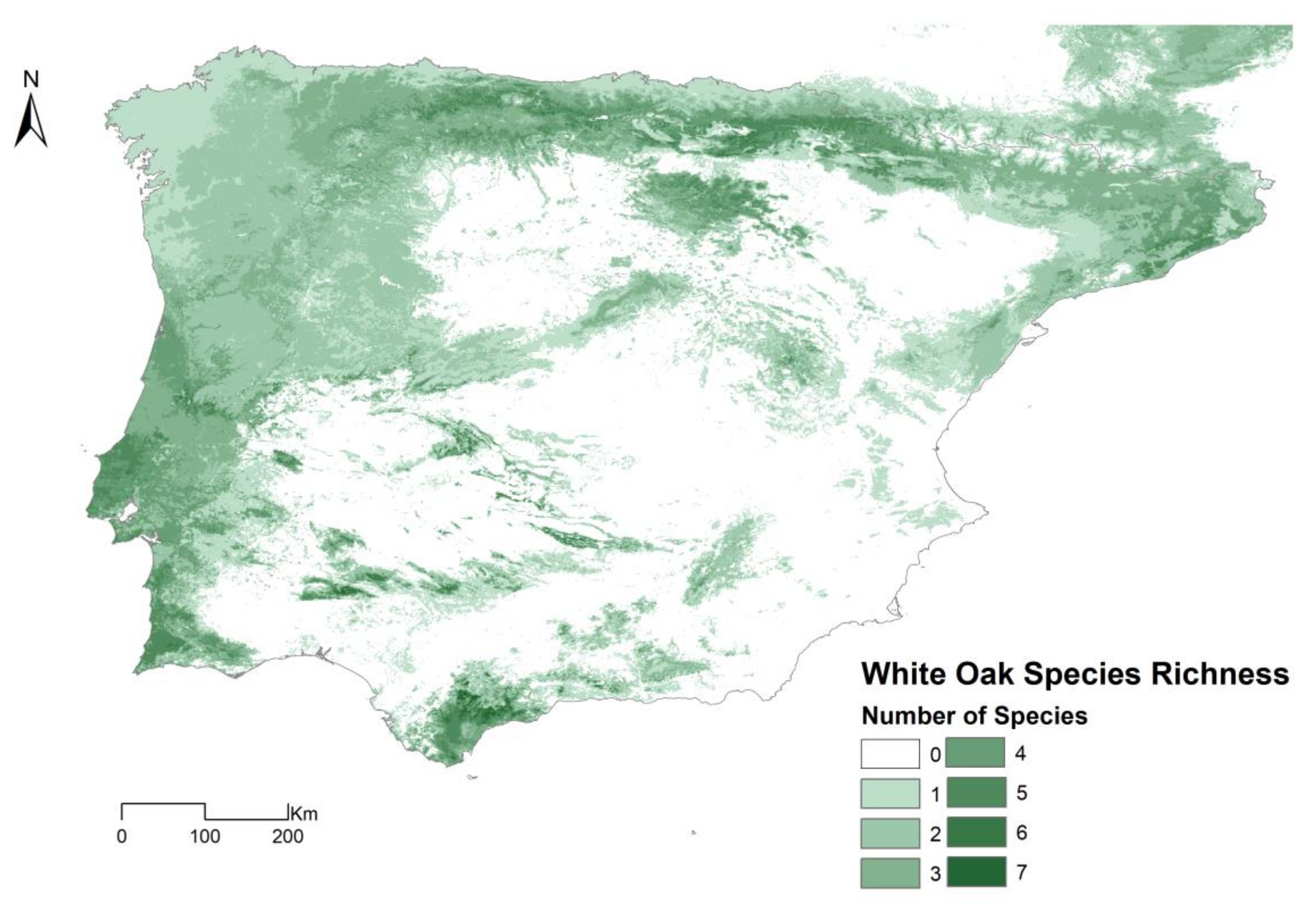
Depict the fittest biogeographic areas for oak conservation based on a species-richness map obtained through stacking individual SDM’s.

2. Materials and Methods

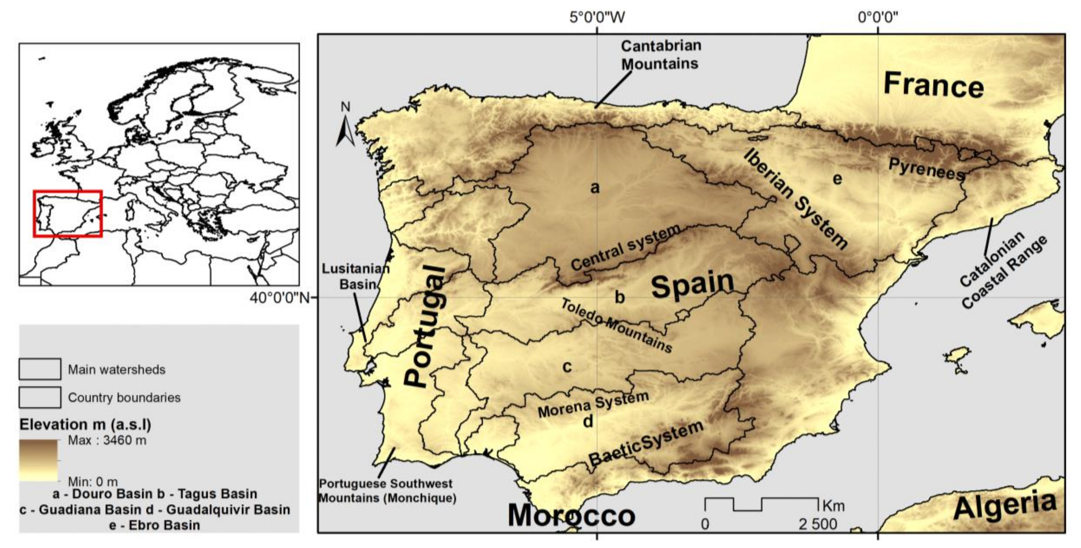
2.1. Study Area

The Iberian Peninsula (IP) is located in southwestern Europe (bounded by longitudes -9.55° W to 3.35° E and latitudes 35.87° N to 43.80° N) and has a total area of 583 832 km² (Figure 1). The region holds a highly diverse geological history [53] and a climate that ranges from a dry Mediterranean in the southeast to a wet Temperate Atlantic in the north [13]. As result of its biogeographic idiosyncrasies and diverse edaphoclimatic conditions, the IP is a major hotspot of European plant diversity, hosting 54% of all European species (22.7% of endemicity), including 21 genera [54] and 13 recognized phylogeographic refugia [55].

2.2. Occurrence Data and Focal Taxa

Oak species geographic information was obtained through extensive fieldwork in western IP (since 2005), classic literature and herbaria review. To tackle taxonomic geographic uncertainty, we gathered the information through the thorough examination of 17 reference herbaria, in more than 6000 vouchers. This info was scrutinized and homogenized with online collections and digital databases (Supplementary Information S1). Geographical records for the target taxa were subsumed and aggregated to a 1 x 1 km grid (Datum WGS1984/UTM30N), using both accurately georeferenced points and UTM grid centroids (Supplementary Information S2). We used ESRI ArcGIS 10.3 for spatial data processing and R version 3.3.1 (R Core Team, 2019) for data management and analysis.

We selected a set of thirteen Iberian White Oaks (Sect. Quercus) [12], which included six roburoid taxa (former Sect. Robur Endlicher [56]) and seven Gall Oaks (subsection Galliferae Gurke) [24,57,58]). This taxonomic set comprises traditional and updated taxonomic approaches, including infraspecific variation and the existence of stabilized nothotaxa (Supplementary Information S3).

2.3. Predictor Variables

2.3.1. Satellite-Based Ecosystem Functioning Attributes (EFAs)

Satellite remote sensing data from the Moderate Resolution Imaging Spectrometer (MODIS) on-board the Terra satellite platform were used to extract EFA variables. The MOD09A1 product, delivering global surface reflectance imagery with 8 days of temporal resolution, 500 m of spatial resolution and with an archive spanning from the year 2000 to the present day, was employed to calculate two spectral indices: (i) the enhanced vegetation index (EVI) [59] as a proxy of vegetation greenness, biomass and leaf area index—with values ranging from −1 to 1, with healthy vegetation generally holding values between 0.20 and 0.80; and (ii) the Normalized Difference Water Index (NDWI) [60] as a proxy for the amount of vegetation and soil water content—with values varying between −1 and +1, with higher values corresponding to high vegetation/soil water content.

To describe the intra-annual properties of each spectral index and aiming to obtain EFAs linked to carbon and water cycles [28,29], we calculated the median (as a descriptor of central tendency and quantity), the inter-quartile range (IQR; as a measure of intra-annual seasonal variation or seasonality) and the sine and cosine transformations of the day of maximum annual value, respectively, related to spring and winter peaks (DMaxSpring or DMaxWinter as a descriptor of phenology). These statistical measures were calculated for each complete year. To capture the multi-year normal conditions of each EFA variable, thus reducing the effect of stochastic annual climatic fluctuations, we computed the overall median. Calculations were performed in Google’s Earth Engine (GEE) cloud-based platform [61]. All 8-day image composites available in the GEE archive spanning from 2001 to 2019 (i.e., all complete years) were used, totalling 873 available images/dates (check Supplementary Information S4). Data were exported from GEE at 1 km of final spatial resolution, totalling eight variables: median, IQR, sine and cosine transformations, and DMax for both EVI and NDWI.

2.3.2. Climatic Data

Bioclimatic variables (derived from monthly temperature and rainfall data to generate more ecologically meaningful variables) were used to portray the temperature and precipitation regimes of the study area. These climatic data were obtained for historical conditions (1970–2000) from the WorldClim dataset version-2.1 (released in January 2020; https://www.worldclim.org/data/worldclim21.html) at a spatial resolution of 30 arc-sec (~1 km). Based on a preliminary assessment (supported by the correlation and variable importance assessment from preliminary models; not shown) [62,63], three temperature-related and two precipitation variables were used, namely: BIO01—Annual Mean Temperature, BIO03—Isothermality, BIO06—Minimum Temperature of Coldest Month, BIO12—Annual Precipitation and, BIO18—Precipitation of Warmest Quarter.

2.4. Model Development, Evaluation and Multi-Algorithm Ensembling

Species distribution models (SDMs) were developed in R statistical software [64] using the biomod2 package [65,66]. This package implements a multi-model ensemble forecasting approach which combines several existing statistical and machine-learning-based algorithms thus enabling to assess and prevent a range of methodological uncertainties in each individual modelling algorithm, as well as the examination of species–environment relationships. Models were fitted using nine modelling techniques: generalized linear model (GLM); generalized boosted model (GBMs); generalized additive model (GAM); classification tree analysis (CTA); artificial neural networks (ANN); flexible discriminant analysis (FDA); multivariate adaptive regression splines (MARS); random forests (RF); and MAXENT.Phillips2 (Maximum Entropy Model), currently available in biomod2. Given the subpar performance of the surface range envelop method (also called BIOCLIM; see e.g., [67]) and the similarity of MAXENT.Phillips (also a maximum entropy-based model available in the biomod2 package) these two algorithms were not considered. Default parameters were employed (with the exception of the smoothing degree term in GAM which was set to k = 4 to prevent over-fitting issues [68] and the number of boosting trees in GBM, n.trees = 2000). Previously to modelling, all candidate variables were inspected for multicollinearity issues using Spearman’s non-parametric pair-wise correlation. By setting a threshold of |ρ| < 0.8, we retained a total of ten variables (out of 13) including: all bioclimatic variables (BIO 01, 03, 06, 12 and 18) and EVI annual median, EVI IQR, EVI DMax-Spring, NDWI median and NDWI IQR. Given that only presence data were available for the selected species, we established a total of five sets of randomly generated pseudo-absences, each set with ten times the number of presence records allowing to diversify environmental conditions in the data used for model training. Since no previous information was available about the species prevalence (p) nor a robust way to accurately estimate it and after checking the comparative results by [69], model weights were adjusted to set p = 0.5 (biomod2 default) thus giving a similar weight to presences and generated pseudo-absences [69]. A spatial thinning procedure implemented in the spThin R package [70] was applied prior to modelling which imposes a minimum spatial separation between input records (through subsampling) with a distance equal to 3 km, thus decreasing autocorrelation and sampling bias effects.

Holdout cross-validation was employed to evaluate the models, with 80% of the input records used for model fitting (train data set) and 20% for model evaluation at each round (test data set). A total of ten rounds were performed for the model evaluation. For assessing the model performance, the area under the receiver-operating curve (ROC), the true-skill statistic (TSS), Cohen’s Kappa (KAPPA) and the sensitivity and the specificity values were calculated [65]. Given that 450 models were generated per species, the less performant models were filtered out before the final ensemble forecasting. Hence, we selected the top 10% percentile best models for the six best performing techniques, considering the TSS rank (n = 30). Based on these top performing models, an ensemble using the average was implemented, thus reducing inter-model uncertainty. To ‘binarize’ projections (to dichotomous suitable/unsuitable habitat) the threshold value maximizing the TSS statistic was used. A linear mixed-effects model was devised through the R package lme4 [71] to check if there was an effect of the set of predictive variables (either the combined set including the climate and EFA variables, climate-only or EFA-only; i.e., fixed factor) on the predictive performance scores (i.e., response variable) while controlling for the species and evaluation metric (i.e., random factors). An ANOVA analysis was then performed to assess if the effect of the set of predictive variables was statistically significant. Finally, given the different number of variables between models setups (partial vs. combined), we also calculated the Akaike information criterion (with finite sample size correction; AICc) for GLM’s allowing to rank models [72,73] while accounting for a different number of variables in each set (i.e., partial climate or satellite EFA’s models vs. combined ones).

3. Results and Discussion

Models Performance and Environmental Predictors

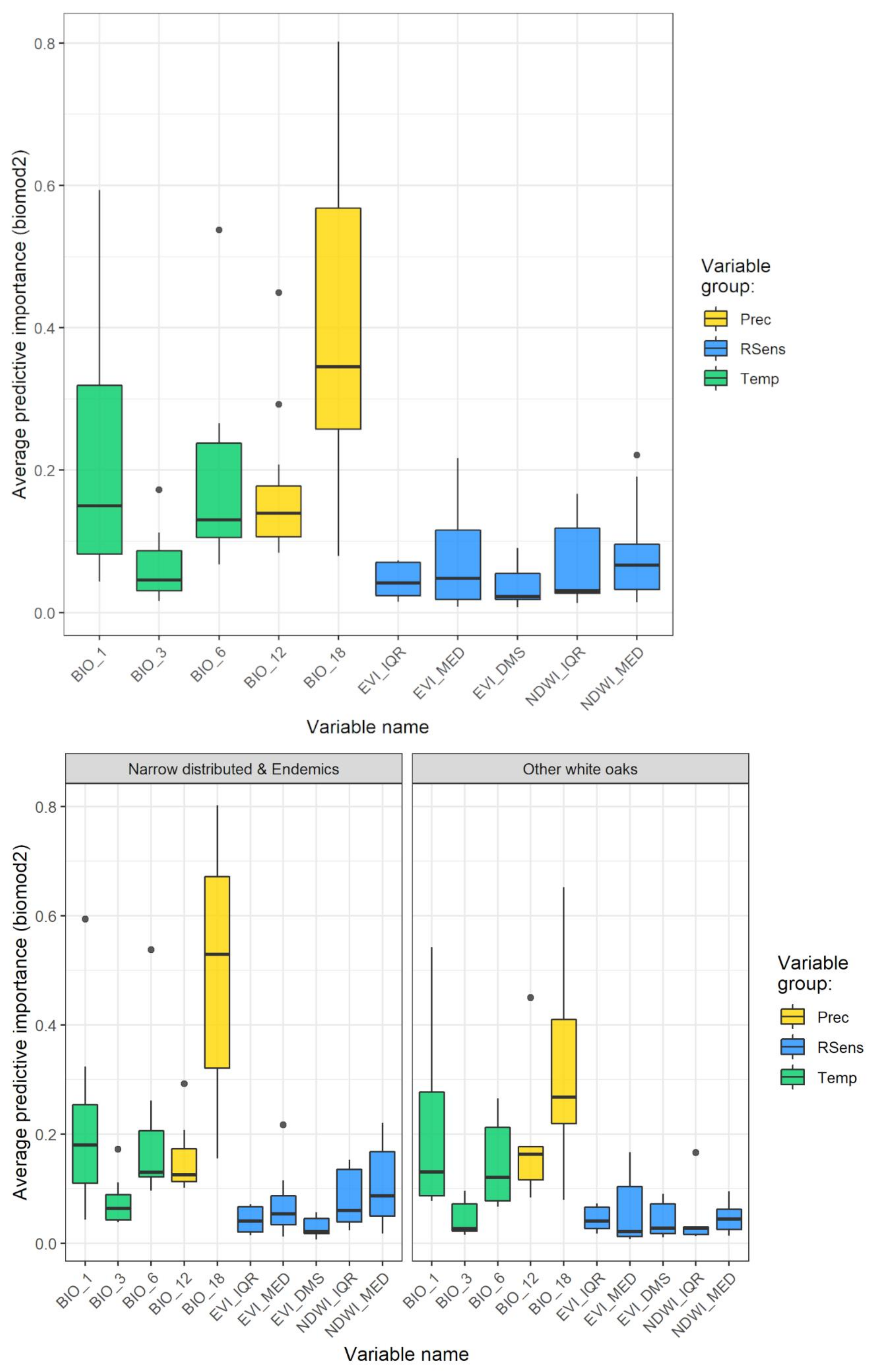
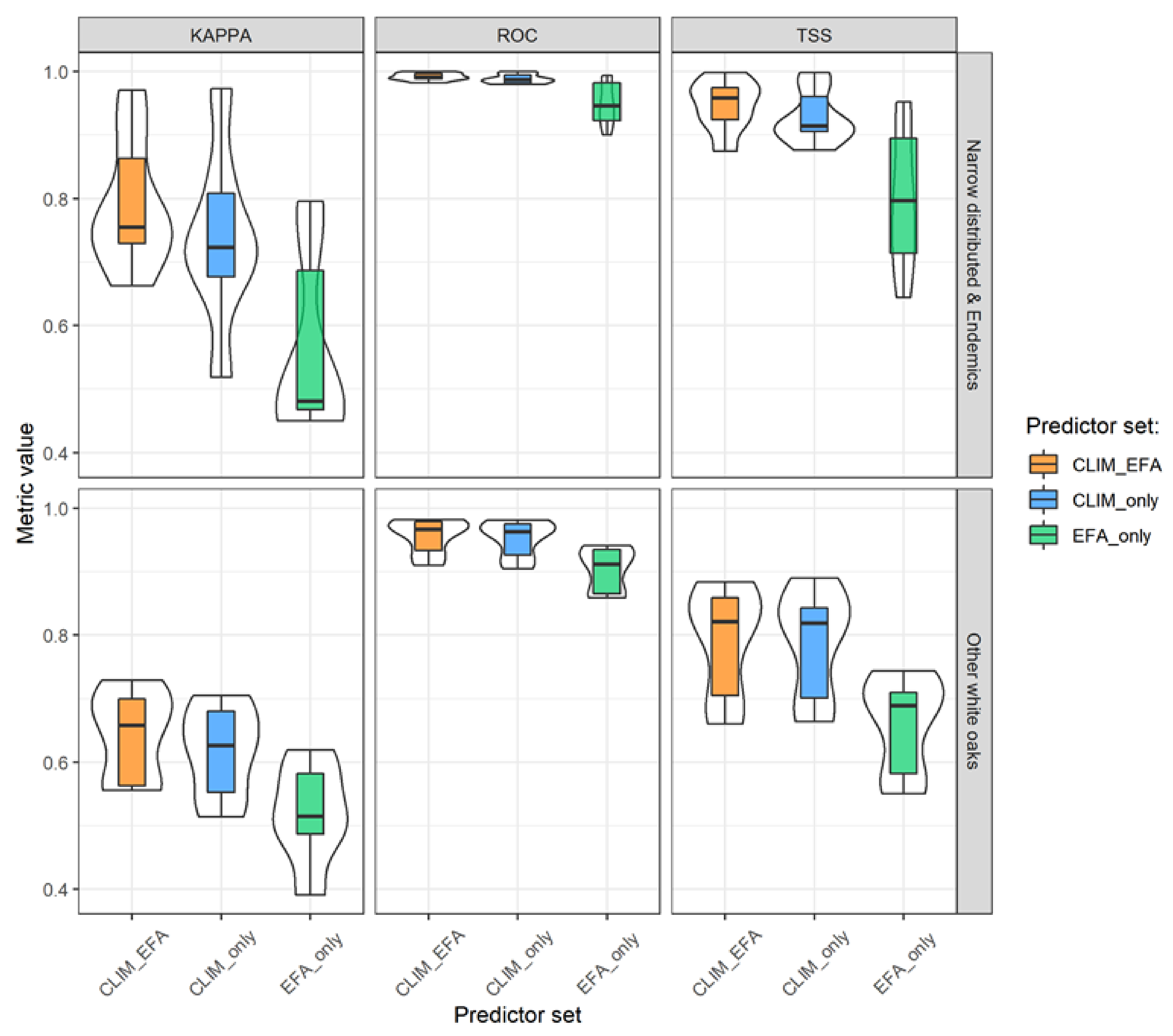
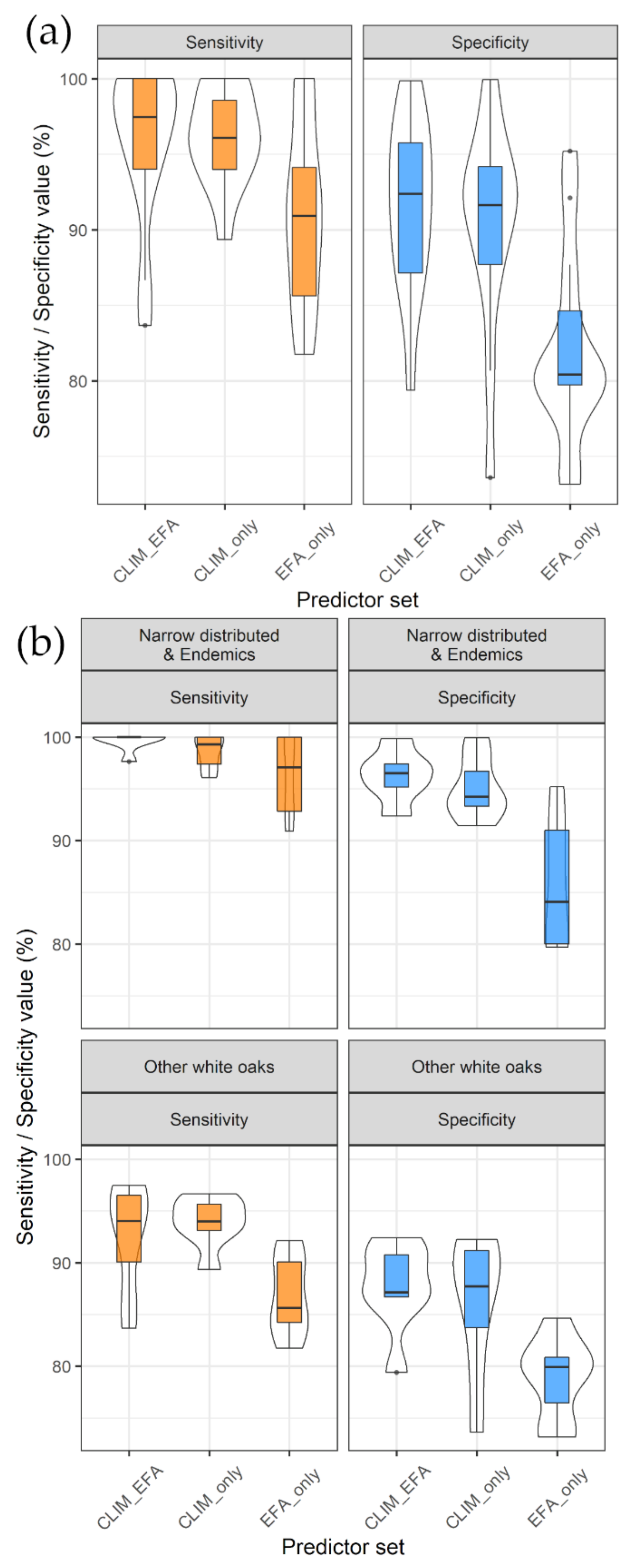
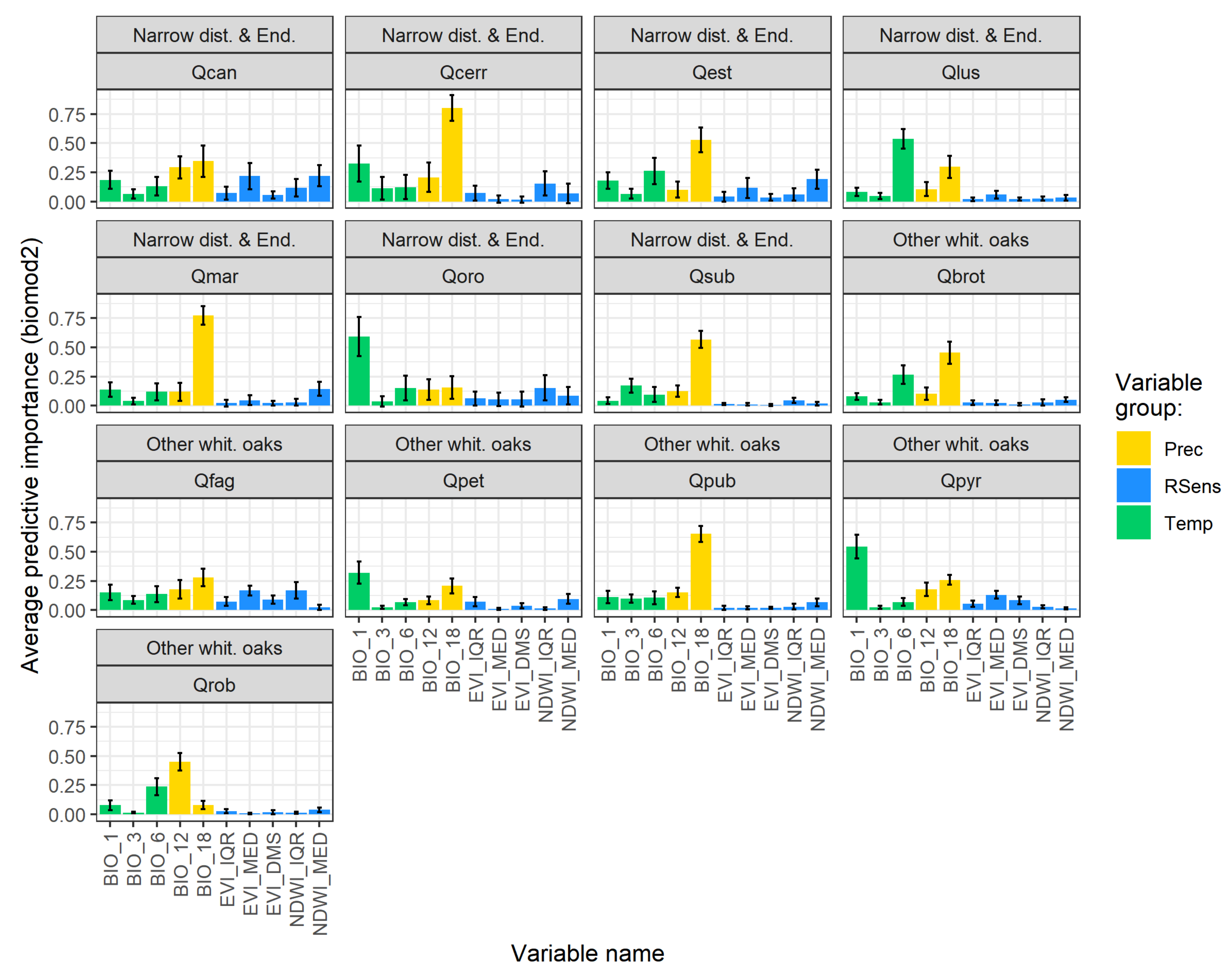
3.1. Model Performance and Added Value of EFAs as Predictors

Overall, the models combining EFAs and climate variables obtained a higher performance and predictive ability (average values for TSS: 0.88, ROC: 0.98, KAPPA: 0.72, sensitivity: 99.6, specificity: 96.3), in comparison to climate-only models (TSS: 0.86, ROC: 0.97, KAPPA: 0.68, sensitivity: 96.1, specificity: 90.3) and EFA-only models (TSS: 0.73, ROC: 0.93, KAPPA: 0.54, sensitivity: 91.2, specificity: 82.1). In addition, narrow endemic species obtained higher predictive performances using combined models (average TSS: 0.96, ROC: 0.99, KAPPA: 0.80, sensitivity: 99.6, specificity: 96.3) in comparison to the widespread oaks (TSS: 0.80, ROC: 0.96, KAPPA: 0.66, sensitivity: 92.6, specificity: 87.7). These results show that the modelling performance for the different sets of variables and taxonomic groups increase in performance when combining Climate and EFA variables for all metrics but especially for Kappa and TSS, whereas ROC is less sensitive to improvements, followed by climate-only and a consistent lower performance for the EFA-only set (Figure 2). This is particularly true for the NDE species-group, with the slightest differences between climate and EFA and climate-only in TSS and ROC for the remaining White Oaks. When comparing performance metrics, it is also important to consider their scale of variation; while Cohen’s Kappa and TSS vary between −1 and 1 (with better models nearing one), ROC varies between 0 and 1 (also with better models nearing one) and hence the later lower ability to discriminate across good performing models holding a lower variance and saturating at the upper-end part of the spectrum. The increase in the performance by the combined set of climate and EFA is also reflected in terms of sensitivity (true positive rate), but especially in terms of specificity (true negative rate) (Figure 3). As before, these gains are reflected especially in the NDE group, and particularly for species such as Q. ×cerrioides, Q. canariensis, Q. orocantabrica and Q. estremadurensis (

Table 1. Evaluation scores per studied species for the ensemble of 30 top-models combining both climate and satellite-based EFA variables (TSS: true skill statistic; ROC: area under the receiver operating curve; KAPPA: Cohen’s Kappa; sensitivity (also called true positive rate or recall); specificity (also defined as the true negative rate)). The number of species records presented are computed after removing duplicates and applying the spatial thinning algorithm for imposing a minimum separation distance of 3 km between points (spThin). * narrow distributed; ** endemic.

Species Names	TSS	ROC	KAPPA	Sensitivity	Specificity	Number of Species Records
Quercus ×cerrioides **	1.00	1.00	0.97	100.0	99.9	18
Quercus canariensis *	0.98	1.00	0.78	100.0	97.5	96
Quercus orocantabrica **	0.97	1.00	0.89	100.0	97.2	33
Quercus estremadurensis *	0.96	0.99	0.66	100.0	95.8	46
Quercus lusitanica *	0.93	0.99	0.72	97.6	95.0	212
Quercus marianica **	0.92	0.99	0.75	100.0	92.4	70
Quercus pubescens	0.88	0.98	0.73	97.5	90.9	473
Quercus subpyrenaica **	0.88	0.98	0.76	96.8	90.6	375
Quercus broteroi	0.86	0.98	0.70	93.5	92.4	306
Quercus robur	0.83	0.97	0.64	96.2	86.8	901
Quercus petraea	0.81	0.97	0.68	94.0	87.1	753
Quercus faginea	0.71	0.93	0.56	83.7	86.6	301
Quercus pyrenaica	0.66	0.91	0.56	86.7	79.4	3282

and Appendix A - Figure A1).

Results from the post hoc ANOVA test based on linear mixed-effects modelling (with a species and evaluation metric as random factors) showed a significant effect of the set of predictive variables on performance scores (p < 0.001). Estimated coefficients show that (despite variability) the “climate-only” and the “EFA-only” sets both have on average less performant models in relation to the combined climate–EFA set, since both coefficients are negative and, respectively, equal to: −0.018 ± 0.015 and −0.124 ± 0.014 (estimate ± std. error). These estimates also show that performance gains are higher in relation to the “EFA-only” set but less in relation to the “climate-only” (see Supplementary Information S5 for more details). The AICc-based model ranking (which measures model fitting performance while accounting for the number of variables in the models; Supplementary Information S6) also showed that for nine (out of thirteen) species, including Q. broteroi, Q. canariensis, Q. ×cerrioides, Q. lusitanica, Q. marianica, Q. orocantabrica, Q. pubescens, Q. pyrenaica and Q. subpyrenaica, better model performances are attained for the climate–EFA combined models. For Q. faginea, Q. petraea and Q. robur the EFA-only models obtained better performances according to the AICc-based ranking, while for Q. estremadurensis the climate-only model was the best one. This evidences that the higher number of variables in combined models (i.e., higher complexity) does not affect the overall ranking.

The consistent better performance of combined climate and EFA models, despite the relatively small increment for some species (Figure 2, Figure 3 and Figure A1), suggests that these two types of variables, when combined, improve the predictive models. Results improved especially for NDE species which have narrower biogeographic ranges and ecological niche breadths. In contrast, models based solely on EFA variables show the lowest performances, even when compared with climate-only models. This may be explained by the coarse scale of the models developed (i.e., with low spatial resolution and a large areal extent) for which regional variations of climate patterns hold substantial more predictive power than finer/local ecosystem functioning patterns depicted by satellite EFA variables. This may be due to the particularly high affinity of most White Oak species to climate gradients, which constrain or control several important physiological aspects of these species’ environmental tolerances at a regional scale [74]. The scale of the influence of variables capturing primary to secondary (or regional to local) patterns structuring species habitat given each one’s spatial autocorrelation patterns, has been previously identified for SDMs [75]. This may also mean that when used at a narrower extent and higher spatial resolution (i.e., finer scale), EFA variables may prove more relevant by their ability to describe small scale variation, heterogeneity and environmental gradients in species habitat patterns, and thus present distinct predictive abilities given species attributes and modelling scale [37].

At a regional/coarser scale, EFAs are mainly driven by climate patterns while in contrast these are more linked to land-cover and land-use patterns at a finer/local scale and thus capturing human influence on ecosystems [36,37,38]. As such, EFAs offer an integrative, quicker and more up-to-date view of ecosystem responses to environmental factors and changes, in comparison to attributes of structure (e.g., patch size, fragmentation) or composition (e.g., percent cover of certain habitats) [36,37,38,76] and thus linking species responses to pressures on ecosystem functioning and its state [38]. This holds advantages for implementing species-monitoring programs [41,77,78] and at the same time, satellite-based EFAs also have the virtue of inserting more ‘realism’ into the spatial predictions of models. For example, implementing EFA variables in models may aid by removing unsuitable areas occupied by artificial or shrubby vegetation (both with a lower mean and seasonal variation in annual EVI or productivity) that may appear as suitable in climate-only models (which solely portray the potential distribution) while in combined models they likely do not. By including integrative, finer-scale attributes of ecosystem functioning linked to each species habitat and suitable environmental conditions, models may better approximate the realized distribution of species which may present several advantages for conservation, management and restoration efforts. Nonetheless, it is important not to blur the distinction between modelling a species distribution or its environmental suitability from actually detecting it through satellite imagery using spectral signatures or indices [79].

A frequent limitation linked to SDMs is that species occurrences (one of SDM’s key inputs) are usually available at coarse resolutions [80] while their conservation and management are often required at a much finer spatial resolution [81,82]. Moreover, many predictive variables are also not measurable or available at the required spatiotemporal resolution and consequently, surrogates and interpolated data (e.g., from weather stations) have to be used instead [83,84]. Structural predictors from thematic maps (e.g., land-cover) also bear limitations by often not representing key landscape features nor the ecosystem processes relevant for characterizing a certain species status and change. Moreover, both occurrence data and predictive variables can have inappropriate or distinct spatial, thematic and/or temporal resolutions which impacts model quality and performance [85].

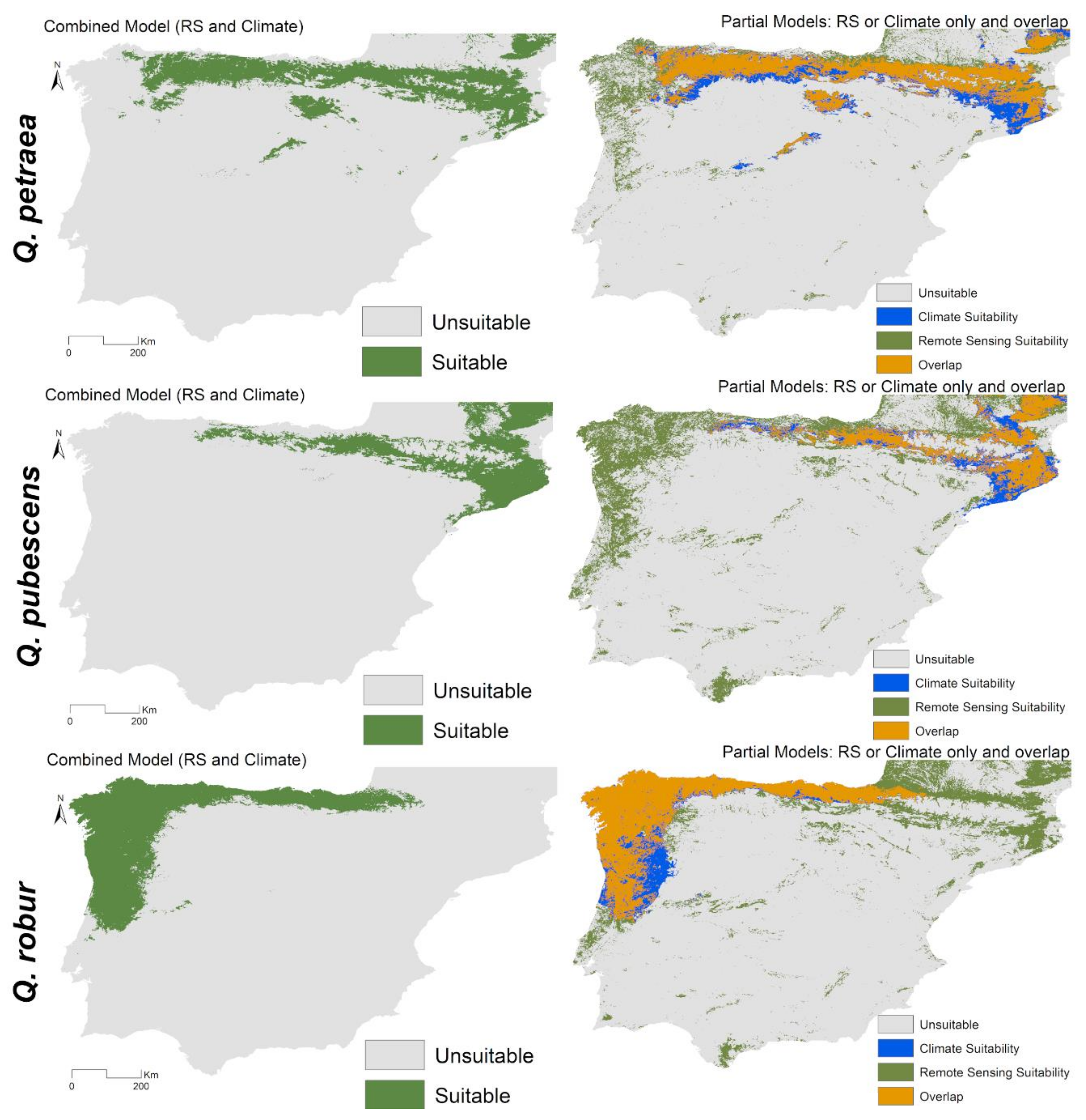
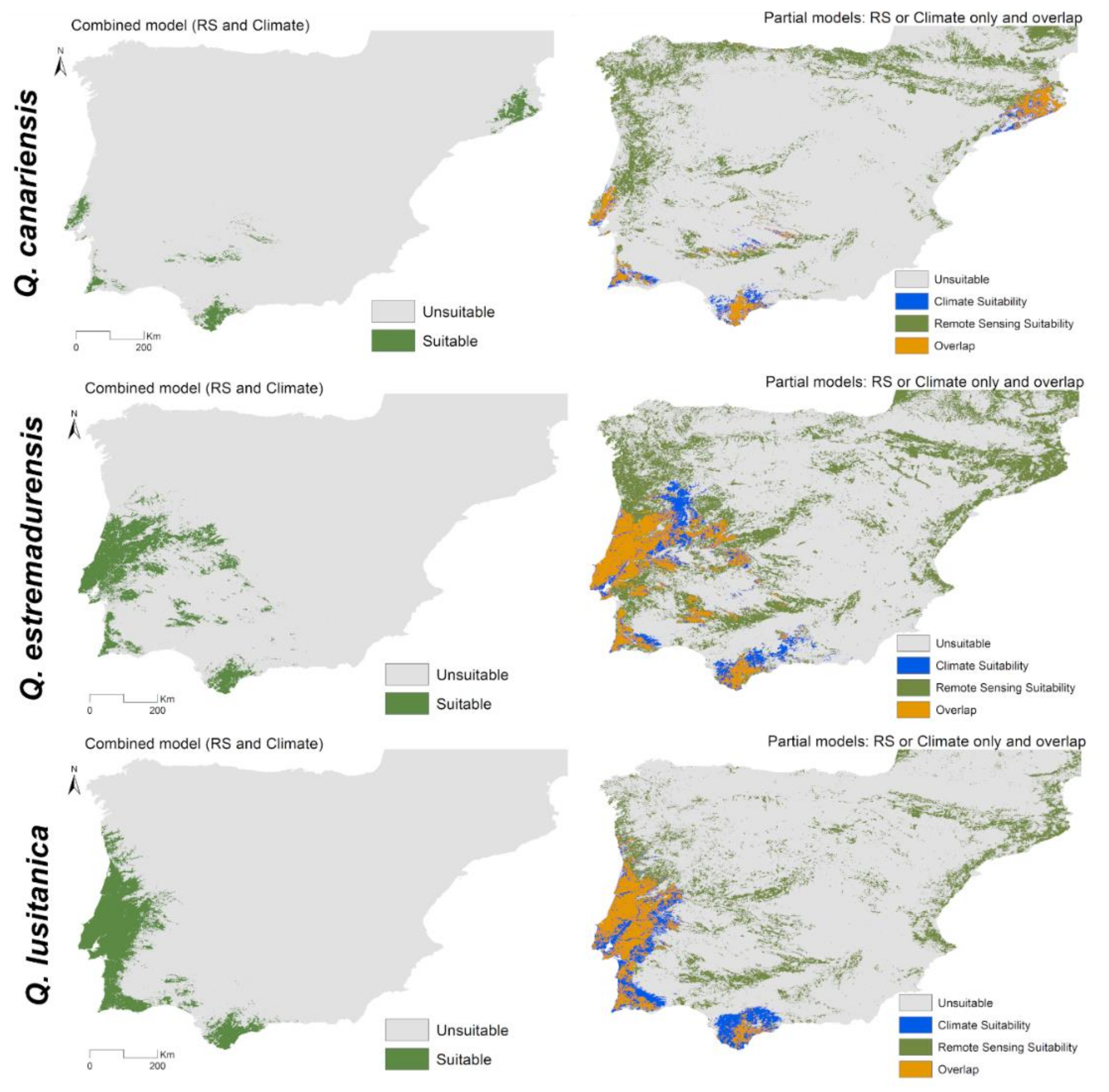
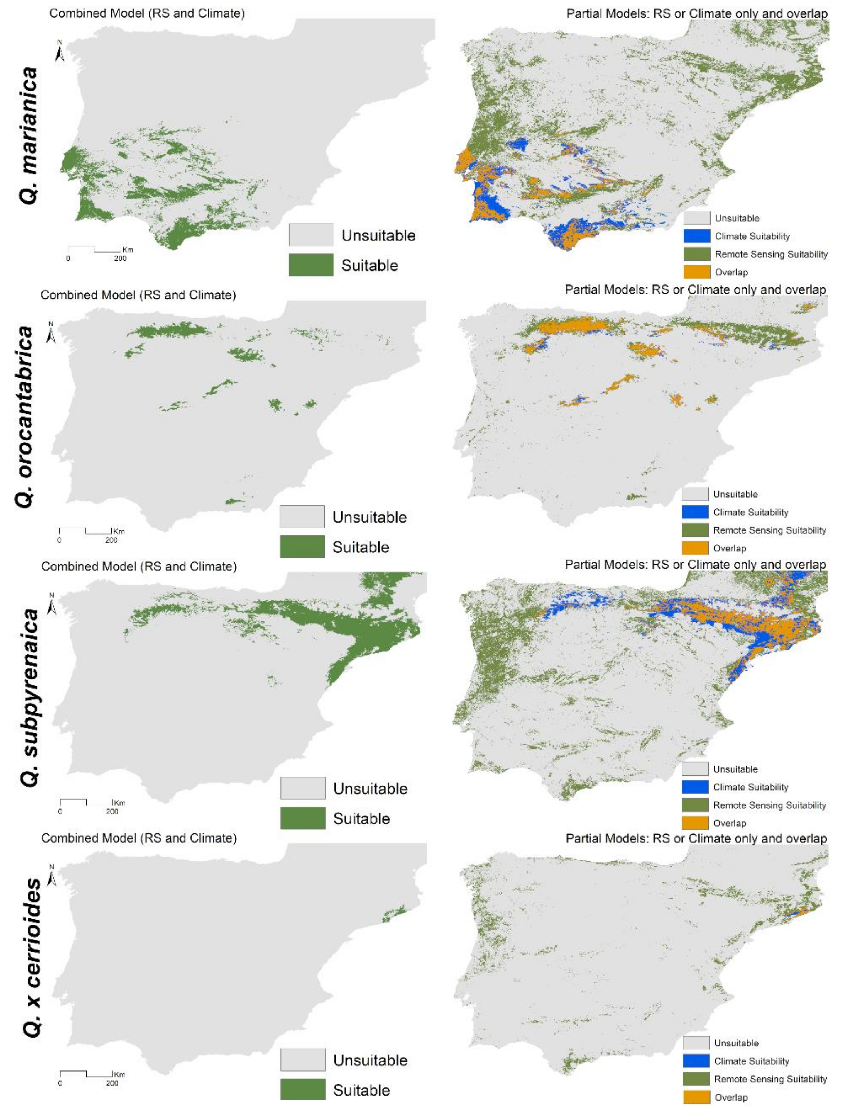
3.2. Combined Models for Individual Species

Overall, combined models (i.e., with both satellite-based EFA and climate variables) showed higher performance scores for all NDE taxa than other White Oaks (TSS > 0.88; Figure 2), especially for Quercus ×cerrioides, Q. canariensis, Q. orocantabrica, and Q. estremadurensis (Table 1). The lowest TSS values corresponded to Q. faginea and Q. pyrenaica (0.71 and 0.66, respectively). ROC values were always above 0.9, suggesting an overall excellent performance of the NDE models. Cohen’s Kappa values (typically more sensitive to true negative rates) varied between 0.56 and 0.97, also showing a strong performance of combined (climate and EFA) models with variations across species. In addition, sensitivity and specificity scores were always above 80% (with a slight exception for the widespread Q. pyrenaica), confirming the good and well-balanced performance of the models (Table 1; Supplementary Information S7).

Generally, we observe a bigger relevance of precipitation-related variables and a fluctuation of the importance of a second group of predictors, either related with temperature, or with EFA variables. When considering all species, climatic variables are generally the most important ones, especially the precipitation of the warmest quarter (BIO18), followed by annual precipitation (BIO12), annual mean temperature (BIO01) and winter cold (BIO06) (Figure 4 and Appendix A - Figure A2). The same pattern is noticeable for the widely distributed White Oaks, but temperature-related variables (BIO01 and BIO06) become the second and third most important variables for the NDE group, followed by BIO12, with NDWI_MED, occupying the fifth position for these group of species (Appendix A - Figure A2).

When taking into account individual species (Figure 4), summer precipitation (BIO18) is predominantly the most important variable for most of the Iberian White Oaks, only superseded by winter cold (BIO6) for Q. lusitanica, annual mean temperature (BIO01) for Q. orocantabrica, Q. petraea and Q. pyrenaica, and annual precipitation (BIO12) for Q. robur. EFA-related variables occupy the third and fourth positions for several NDE oaks, like Q. canariensis, Q. ×cerrioides, Q. marianica, Q. estremadurensis and Q. orocantabrica, especially EVI_MED and NDWI_MED. Q. faginea seems to be the species with the most balanced equilibrium between variables (Figure 4).

Regarding EFAs, its contribution was found to be more important as predictors in models of NDE species than other White Oak species as before, regarding model performances. More specifically, the inter-quartile range of the NDWI (a descriptor of seasonality in water balance/content) was the most relevant variable across all of the studied species, followed by the median of NDWI and EVI (descriptors of water balance/content and primary productivity, respectively) (Figure 4).

These results reflect the high dependence of precipitation for these group of oaks, especially in the dry season (BIO18) for most of the Gall Oaks, or those geographically distributed throughout the sub-Mediterranean and southern areas of the IP. The winter cold (BIO06) importance explains the distribution of Q. lusitanica in the Atlantic shore of the IP, showing this species’ intolerance for winter cold, while the annual precipitation (BIO12) marks the distribution of Q. robur as it cannot withstand low precipitation levels and summer drought. The third and fourth position occupied by EFA predictors for some NDE species, represent the importance of the vegetation state/quality, for the maintenance of some of these oaks, especially for the relicts Q. canariensis and Q. estremadurensis and the endemics Q. ×cerrioides and Q. marianica. These taxa are dependent on shady and moist environments, normally in deep canyons of Atlantic areas. Herein, EVI-related EFA’s were found suitable to depict primary production and water availability patterns of these areas with higher levels of humidity linked to the maintenance of these species [86,87,88,89].

The visual inspection of suitability maps for the seven NDE taxa shows the best areas for the preservation and recovery of the selected species. Here, we can compare the combined model (with satellite EFA and climate variables), with the spatial overlap of partial models (RS and climate) (Figure 5 and Figure 6). Overall, the contribution of EFA predictors brings higher accuracy for the spatial delimitation of these species’ recovery areas, by reflecting the vegetation state through primary productivity and moisture conditions (better captured by NDWI-related EFA variables), and by adding it to the climatic suitability for each species.

When analysing the narrowly-distributed oaks (Figure 5), Q. canariensis evidences suitable environmental conditions in its “typical” locations, from the Iberian southwest (Monchique and Algeciras) and Catalonian sub-populations, with the maintenance of residual areas in Morena System and suitable areas and Littoral shore of Centre Portugal (around Lisbon) (Figure 1). A similar pattern is followed by Q. estremadurensis, with a wider suitable area, through central Portugal up to Montes de Toledo (Spain) and an incursion in the Portuguese Douro thermophilic areas. Q. lusitanica preserves most of its known distribution [7,9], with the overlap of partial models being considerably smaller than the combined models (Figure 5).

When looking at endemic oaks (Figure 6), Q. marianica shows a larger suitable area with a higher ecological plasticity in comparison to its parental species Q. canariensis, extending throughout Morena mountain chain and the western Portuguese coast. By tracking the remaining parental species (Q. broteroi) it enhances the role of hybridization by adapting to new ecological conditions as a strategy for survival in growing drier habitat types and conditions, where at least one of the parentals lost fitness (Q. canariensis) [90,91]. Q. orocantabrica shows a wider area out of its currently known range, across the Cantabrian mountains and three disjoint subpopulations in Rioja, Cuenca and the Central system (Figure 1), with the EFA predictors contributing to diagnose orophile conditions in the suitable environmental space. These novel spatial inferences may in turn help managers and stakeholders to devise much-needed restauration, recovery or re-introduction efforts [92,93,94,95]. Likewise, Q. marianica, the nothotaxa Q. subpyrenaica, show a wider and more continuous distribution in comparison to the parental Q. pubescescens (see Appendix A - Figure A4), however, in reverse, a more reticulated distribution in the overlap of the partial models. This shows a higher ecological plasticity by matching the other parental species (Q. faginea) and tracking the sub-Mediterranean belt of northeast IP, while Q. pubescens presents a more continuous temperate distribution in the partial models and a reticulated distribution in the combined ones, being a more restrict taxon in terms of distribution. The endemic nothotaxa Q. ×cerrioides has a reduced suitable area in the littoral Catalonian mountains, as it results from contact with the residual Q. canariensis forests.

The remaining Iberian White Oaks, with wider distributions, frequently present smaller overlap areas between partial models than the combined ones, highlighting more detailed areas where to recover this species group when taking into account the EFA predictors (Appendix A - Figure A3 and Figure A4). The Quercus broteroi combined model shows a continuous area in western Iberia and throughout the Morena System and Montes de Toledo, with the overlap of partial models evidencing the best areas for this species recovery. By opposite, Q. faginea combined models show a wider area in the Douro Basin and throughout the Cantabrian mountains, Iberian and Betic Systems, and eastern IP, while the overlap shows a more conservative area for its recovery (Figure 1). Likewise, Q. pyrenaica presents a similar pattern, while including the central system and northwest Iberian mountain areas, with disjoint relict subpopulations in southern Iberia. Q. petraea and Q. robur present complementary projected areas that reflect their ecological requirements, both with a larger overlap between combined models and the overlap of partial models. Q. pubescens shows similar patterns of the nothotaxa Q. subpyrenaica, with the first having a temperate distribution while the second enters into sub-Mediterranean areas [14,96]. Both species evidence notorious differences between the combined models when in comparison to the overlap of the partial ones, with larger areas in the first ones.

3.3. Spatial Projections and Patterns of Species Richness

Model projections for all Iberian White Oak species (Figure 7) reveal areas with cumulative suitability up to seven oak taxa, highlighting the Iberian southwest mountains, the Lusitanian Basin, Montes de Toledo and to sub-littoral Catalonian mountains (Figure 1) as highly relevant. These areas can be considered the largest hotspots and the most important “lost” areas for the Iberian White Oaks conservation, being suitable for the highest diversity of oak taxa. Oaks in general show strong niche conservatism [74], particularly the Subgenus Quercus [12], that comprises temperate lineages of oaks [97], which were heavily constrained in the IP by its biogeography, prevailing only in areas with similar climates. This way water availability and the Atlantic influence plays a major role, especially when in a seasonal climate like the Mediterranean one [13]. Thus, our study provides a lacking approach to assess these woody temperate plants species richness which can provide useful data for promoting their persistence [98], while unveiling the importance of multiple drivers of ecosystem functioning and their interaction with the climate in a biogeographic transitional area between Temperate and Mediterranean Europe.

Such results allow to better understand the co-distribution and the spatial patterns of potential species richness of these taxa and therefore to know and prioritize areas with higher biogeographic conservation value. The central and western IP show the best areas for the Gall Oaks, where Q. canariensis, Q. broteroi, Q. lusitanica and Q. marianica have suitable environmental conditions to co-occur, together with Q. estremadurensis, which is a relict species, and also the presence of the widespread Q. pyrenaica, that in these thermophilic areas is also rare but potentially distributed. This area is only matched by the littoral Catalonian range, where Q. canariensis co-occurs with the roburoid Q. pubescens, Q. petraea and Q. robur, with an intricated legacy of introgression [28]. This pattern is also present in the pre-Pyrenees area, where Q. subpyrenaica marks the transition from the submediterraenan to the temperate belt alongside the contact of Q. pubescens and Q. faginea. The northern and western mountain ranges, including the Iberian, Cantabrian and Gallaecian Systems are also quite important for the preservation of the European southernmost suitable areas for Q. robur, Q. petraea and the endemic Q. orocantabrica. Moreover, this area has a major relevance for the evolutionary history of these group of oaks in terms of the European forests [11] and their inherent relevance for forest conservation when confronted with projected climatic shifts.

4. Conclusions

We highlighted the importance of incorporating satellite-derived ecosystem functioning attributes for mapping the potential distribution and habitat suitability of oak species, especially to those with a narrow distribution and relict-like character (NDE), in a biodiversity hotspot such as the Iberian Peninsula. Our results show that EFAs are able to improve predictions of the distribution of both narrow- and wide-ranged oak species at the regional scale, and confirm its robustness as predictors of habitat features that complement the climate influence by describing relevant complementary dimensions of the carbon cycle and water balance at the ecosystem level. Thus, satellite-based predictors such as EFAs can nowadays be computed from imagery available at high frequencies and several spatial resolutions, which allow to match the scale of the relevant processes in each study, and to anticipate species’ responses to different disturbances. By doing this, our combined modelling framework illustrates the great potential of EFAs to contribute for monitoring and conservation through the essential biodiversity variables framework (EBV class ‘ecosystem function’).

By incorporating and combining these variables with climatic data, our work addresses the best areas for the conservation of each taxa, for which vegetation state and ecosystem functioning attributes are generally overseen in climate-only studies. The good performance of the models helped to predict the best areas for the preservation of the studied species, while variable importance measures aided to explain the main factors behind species’ distributions in the geographic space. Therefore, this work also serves as base for forecasting the impact of climate change in the Iberian oak forests, in the face of future scenarios. Furthermore, our methodology proved to be suitable to be applied to analogous situations and throughout the Mediterranean Basin and targeting oak forests worldwide. This is of paramount importance in a group characterized by a complex and reticulate evolutionary history. Globally, our results show that species distribution models are a suitable tool to accurately predict oak species distribution which holds great potential to accurately depict the ‘best’ areas for the conservation of the studied taxa. Our study highlights the Iberian Southwest, the Lusitanian Basin and the Catalonian littoral mountains, as the most important biogeographic areas, with greater overall habitat suitability for a larger number of species, functioning as hotspots and relict-like areas for the broad-scale conservation of the Iberian White Oaks.

References

1. Manos, P.S.; Doyle, J.J.; Nixon, K.C. Phylogeny, biogeography, and processes of molecular differentiation in Quercus subgenus Quercus (Fagaceae). Mol. Phylogenet. Evol. 1999, 12, 333–349. [Google Scholar] [CrossRef] [PubMed] [Green Version]
2. Sabatini, F.M.; Burrascano, S.; Keeton, W.S.; Levers, C.; Lindner, M.; Pötzschner, F.; Verkerk, P.J.; Bauhus, J.; Buchwald, E.; Chaskovsky, O. Where are Europe’s last primary forests? Divers. Distrib. 2018, 24, 1426–1439. [Google Scholar] [CrossRef] [Green Version]
3. Anderegg, W.R.; Trugman, A.T.; Badgley, G.; Anderson, C.M.; Bartuska, A.; Ciais, P.; Cullenward, D.; Field, C.B.; Freeman, J.; Goetz, S.J. Climate-driven risks to the climate mitigation potential of forests. Science 2020, 368, eaaz7005. [Google Scholar] [CrossRef] [PubMed]
4. Neophytou, C.; Aravanopoulos, F.A.; Fink, S.; Dounavi, A. Detecting interspecific and geographic differentiation patterns in two interfertile oak species (Quercus petraea (Matt.) Liebl. and Q. robur L.) using small sets of microsatellite markers. For. Ecol. Manag. 2010, 259, 2026–2035. [Google Scholar] [CrossRef] [Green Version]
5. Cramer, W.; Guiot, J.; Fader, M.; Garrabou, J.; Gattuso, J.-P.; Iglesias, A.; Lange, M.A.; Lionello, P.; Llasat, M.C.; Paz, S. Climate change and interconnected risks to sustainable development in the Mediterranean. Nat. Clim. Chang. 2018, 8, 972–980. [Google Scholar] [CrossRef] [Green Version]
6. Balzan, M.V.; Hassoun, A.E.R.; Aroua, N.; Baldy, V.; Bou Dagher, M.; Branquinho, C.; Dutay, J.C.; El Bour, M.; Médail, F.; Mojtahid, M.; et al. Ecosystems; Union for the Mediterranean, Plan Bleu, UNEP/MAP: Marseille, France, 2020; p. 151. [Google Scholar]
7. Franco, J.A. Quercus L. In Flora Iberica, (Plantanaceae-Plumbaginaceae [Partim]); Castroviejo, S., Ed.; Real Jardín Botánico, CSIC: Madrid, Spain, 1990; Volume 2, pp. 15–36. [Google Scholar]
8. Schwarz, O. Quercus L. In Flora Europaea; Tutin, T.G., Heywood, V.H., Burges, N.A., Valentine, D.H., Walters, S.M., Webb, D.A., Eds.; Cambridge University Press: Cambridge, UK, 1964; Volume 1, pp. 61–64. [Google Scholar]
9. Rivas-Martínez, S.; Saénz, C. Enumeración de los Quercus de la Península Ibérica. Rivasgodaya 1991, 6, 101–110. [Google Scholar]
10. Coutinho, A.X.P. Os Quercus de Portugal. Boletim Sociedade Broteriana 1888, 6, 47–116. [Google Scholar]
11. Olalde, M.; Herrán, A.; Espinel, S.; Goicoechea, P.G. White oaks phylogeography in the Iberian Peninsula. For. Ecol. Manag. 2002, 156, 89–102. [Google Scholar] [CrossRef] [Green Version]
12. Denk, T.; Grimm, G.W.; Manos, P.S.; Deng, M.; Hipp, A.L. An updated infrageneric classification of the oaks: Review of previous taxonomic schemes and synthesis of evolutionary patterns. In Oaks Physiological Ecology. Exploring the Functional Diversity of Genus Quercus L.; Springer: Berlin/Heidelberg, Germany, 2017; pp. 13–38. [Google Scholar]
13. Rivas-Martínez, S.; Penas, A.; del Río, S.; González, T.; Rivas-Sáenz, S. Bioclimatology of the Iberian Peninsula and the Balearic Islands. In The Vegetation of the Iberian Peninsula; Loidi, J., Ed.; Springer: Utrecht, The Netherlands, 2017; pp. 29–80. [Google Scholar]
14. De Dios, R.S.; Benito-Garzón, M.; Sainz-Ollero, H. Present and future extension of the Iberian submediterranean territories as determined from the distribution of marcescent oaks. Plant Ecol. 2009, 204, 189–205. [Google Scholar] [CrossRef]
15. Del Río, S.; Penas, Á. Potential distribution of semi-deciduous forests in Castile and Leon (Spain) in relation to climatic variations. Plant Ecol. 2006, 185, 269–282. [Google Scholar]
16. Vila-Viçosa, C.; Gonçalves, J.; Honrado, J.; Lomba, A.; Silva, R.; Vázquez, F.M.; García, C. Late Quaternary range shifts of marcescent oaks unveil the dynamics of a major biogeographic transition in southern Europe. Sci. Rep. 2020. Accepted. [Google Scholar]
17. IPCC. Summary for Policymakers. In Climate Change 2014: Mitigation of Climate Change. Contribution of Working Group III to the Fifth Assessment Report of the Intergovernmental Panel on Climate Change; Pachauri, R.K., Meyer, L.A., Eds.; Cambridge University Press: Cambridge, UK; New York, NY, USA, 2014. [Google Scholar]
18. García-Valdés, R.; Svenning, J.C.; Zavala, M.A.; Purves, D.W.; Araujo, M.B. Evaluating the combined effects of climate and land-use change on tree species distributions. J. Appl. Ecol. 2015, 52, 902–912. [Google Scholar] [CrossRef]
19. Senf, C.; Seidl, R. Mapping the coupled human and natural disturbance regimes of Europe’s forests. bioRxiv 2020. [Google Scholar] [CrossRef] [Green Version]
20. McVay, J.D.; Hipp, A.L.; Manos, P.S. A genetic legacy of introgression confounds phylogeny and biogeography in oaks. Proc. R. Soc. B 2017, 284, 20170300. [Google Scholar] [CrossRef] [PubMed] [Green Version]
21. Hipp, A.L. Should hybridization make us skeptical of the oak phylogeny. Int. Oak J. 2015, 26, 9–18. [Google Scholar]
22. Vicioso, C. Revisión del Género Quercus en España; Tipografía Artítica: Madrid, Spain, 1950; p. 194. [Google Scholar]
23. Vasconcellos, J.C.; Franco, J.A. Os Carvalhos de Portugal. Anais Instituto Superior Agronomia 1954, 21, 1–135. [Google Scholar]
24. del Huget Villar, E. Estudios sobre los Quercus del Oeste mediterráneo. Anales Instituto Botanico A.J. Cavanilles 1958, 15, 3–114. [Google Scholar]
25. Schwarz, O. Einige neue Eichen des Mediterrangebiets und Vorderasiens. Notizblatt Königl. botanischen Gartens Museums Berlin 1935, 114, 461–469. [Google Scholar] [CrossRef]
26. Montserrat, P. Algunos aspectos de la diferenciación sistemática de los Quercus ibéricos. In Simposio de Biogeografía Ibérica; Instituto de Biologia Aplicada: Barcelona, Spain, 1957; Volume 26, pp. 61–75. [Google Scholar]
27. Vila-Viçosa, C.; Vázquez, F.M.; Meireles, C.; Pinto-Gomes, C. Taxonomic peculiarities of marcescent oaks (Quercus, Fagaceae) in Southern Portugal. Lazaroa 2014, 35, 139–153. [Google Scholar] [CrossRef] [Green Version]
28. Schwarz, O. Sobre los Quercus catalanes del subgénero Lepidobalanus Oerst. Cavanillesia 1936, 8, 65–100. [Google Scholar]
29. Rivas-Martínez, S.; González-Días, T.E.; González, F.F.; Loidi, J.J.; Lousã, M.F.; Merino, Á.P. Vascular plant communities of Spain and Portugal: Addenda to the syntaxonomical checklist of 2001. Part II. Itinera Geobot. 2002, 15, 433–922. [Google Scholar]
30. Rodríguez-Sánchez, F.; Hampe, A.; Jordano, P.; Arroyo, J. Past tree range dynamics in the Iberian Peninsula inferred through phylogeography and palaeodistribution modelling: A review. Rev. Palaeobot. Palynol. 2010, 162, 507–521. [Google Scholar] [CrossRef]
31. Guisan, A.; Tingley, R.; Baumgartner, J.B.; Naujokaitis-Lewis, I.; Sutcliffe, P.R.; Tulloch, A.I.; Regan, T.J.; Brotons, L.; McDonald-Madden, E.; Mantyka-Pringle, C. Predicting species distributions for conservation decisions. Ecol. Lett. 2013, 16, 1424–1435. [Google Scholar] [CrossRef] [PubMed]
32. Guisan, A.; Thuiller, W.; Zimmermann, N.E. Habitat Suitability and Distribution Models: With Applications in R.; Cambridge University Press: Cambridge, UK, 2017. [Google Scholar]
33. Luque, S.; Pettorelli, N.; Vihervaara, P.; Wegmann, M. Improving biodiversity monitoring using satellite remote sensing to provide solutions towards the 2020 conservation targets. Methods Ecol. Evol. 2018, 9, 1784–1786. [Google Scholar] [CrossRef] [Green Version]
34. Alcaraz-Segura, D.; Cabello, J.; Paruelo, J.M.; Delibes, M. Use of descriptors of ecosystem functioning for monitoring a national park network: A remote sensing approach. Environ. Manag. 2009, 43, 38–48. [Google Scholar] [CrossRef] [PubMed]
35. Alcaraz, D.; Paruelo, J.; Cabello, J. Identification of current ecosystem functional types in the Iberian Peninsula. Glob. Ecol. Biogeogr. 2006, 15, 200–212. [Google Scholar] [CrossRef]
36. Arenas-Castro, S.; Regos, A.; Gonçalves, J.F.; Alcaraz-Segura, D.; Honrado, J. Remotely sensed variables of ecosystem functioning support robust predictions of abundance patterns for rare species. Remote Sens. 2019, 11, 2086. [Google Scholar] [CrossRef] [Green Version]
37. Arenas-Castro, S.; Gonçalves, J.; Alves, P.; Alcaraz-Segura, D.; Honrado, J.P. Assessing the multi-scale predictive ability of ecosystem functional attributes for species distribution modelling. PLoS ONE 2018, 13, e0199292. [Google Scholar] [CrossRef] [Green Version]
38. Alcaraz-Segura, D.; Lomba, A.; Sousa-Silva, R.; Nieto-Lugilde, D.; Alves, P.; Georges, D.; Vicente, J.R.; Honrado, J.P. Potential of satellite-derived ecosystem functional attributes to anticipate species range shifts. Int. J. Appl. Earth Obs. Geoinf. 2017, 57, 86–92. [Google Scholar] [CrossRef]
39. Pereira, H.M.; Ferrier, S.; Walters, M.; Geller, G.N.; Jongman, R.; Scholes, R.J.; Bruford, M.W.; Brummitt, N.; Butchart, S.; Cardoso, A. Essential biodiversity variables. Science 2013, 339, 277–278. [Google Scholar] [CrossRef] [Green Version]
40. Gonçalves, J.; Alves, P.; Pôças, I.; Marcos, B.; Sousa-Silva, R.; Lomba, Â.; Honrado, J.P. Exploring the spatiotemporal dynamics of habitat suitability to improve conservation management of a vulnerable plant species. Biodivers. Conserv. 2016, 25, 2867–2888. [Google Scholar] [CrossRef]
41. Regos, A.; Gómez-Rodríguez, P.; Arenas-Castro, S.; Tapia, L.; Vidal, M.; Domínguez, J. Model-Assisted Bird Monitoring Based on Remotely Sensed Ecosystem Functioning and Atlas Data. Remote Sens. 2020, 12, 2549. [Google Scholar] [CrossRef]
42. Sun, S.; Zhang, Y.; Huang, D.; Wang, H.; Cao, Q.; Fan, P.; Yang, N.; Zheng, P.; Wang, R. The effect of climate change on the richness distribution pattern of oaks (Quercus L.) in China. Sci. Total Environ. 2020, 744, 140786. [Google Scholar] [CrossRef] [PubMed]
43. Hernández-Lambraño, R.E.; de la Cruz, D.R.; Sánchez-Agudo, J.Á. Spatial oak decline models to inform conservation planning in the Central-Western Iberian Peninsula. For. Ecol. Manag. 2019, 441, 115–126. [Google Scholar] [CrossRef]
44. Vessella, F.; López-Tirado, J.; Simeone, M.C.; Schirone, B.; Hidalgo, P.J. A tree species range in the face of climate change: Cork oak as a study case for the Mediterranean biome. Eur. J. For. Res. 2017, 136, 555–569. [Google Scholar] [CrossRef]
45. Matías, L.; Abdelaziz, M.; Godoy, O.; Gómez-Aparicio, L. Disentangling the climatic and biotic factors driving changes in the dynamics of Quercus suber populations across the species latitudinal range. Divers. Distrib. 2019, 25, 524–535. [Google Scholar] [CrossRef] [Green Version]
46. Noce, S.; Collalti, A.; Santini, M. Likelihood of changes in forest species suitability, distribution, and diversity under future climate: The case of Southern Europe. Ecol. Evol. 2017, 7, 9358–9375. [Google Scholar] [CrossRef]
47. Ülker, E.D.; Tavşanoğlu, Ç.; Perktaş, U. Ecological niche modelling of pedunculate oak (Quercus robur) supports the ‘expansion–contraction’model of Pleistocene biogeography. Biol. J. Linn. Soc. 2017, 123, 338–347. [Google Scholar] [CrossRef]
48. López-Tirado, J.; Hidalgo, P.J. Predicting suitability of forest dynamics to future climatic conditions: The likely dominance of Holm oak [Quercus ilex subsp. ballota (Desf.) Samp.] and Aleppo pine (Pinus halepensis Mill.). Ann. For. Sci. 2018, 75, 19. [Google Scholar] [CrossRef] [Green Version]
49. Duque-Lazo, J.; Navarro-Cerrillo, R.; Ruíz-Gómez, F. Assessment of the future stability of cork oak (Quercus suber L.) afforestation under climate change scenarios in Southwest Spain. For. Ecol. Manag. 2018, 409, 444–456. [Google Scholar] [CrossRef]
50. Ahrends, A.; Rahbek, C.; Bulling, M.T.; Burgess, N.D.; Platts, P.J.; Lovett, J.C.; Kindemba, V.W.; Owen, N.; Sallu, A.N.; Marshall, A.R. Conservation and the botanist effect. Biol. Conserv. 2011, 144, 131–140. [Google Scholar] [CrossRef]
51. Coleman, C.O.; Radulovici, A.E. Challenges for the future of taxonomy: Talents, databases and knowledge growth. Megataxa 2020, 1, 28–34. [Google Scholar] [CrossRef] [Green Version]
52. Ely, C.V.; de Loreto Bordignon, S.A.; Trevisan, R.; Boldrini, I.I. Implications of poor taxonomy in conservation. J. Nat. Conserv. 2017, 36, 10–13. [Google Scholar]
53. Loidi, J. Introduction to the Iberian Peninsula, General Features: Geography, Geology, Name, Brief History, Land Use and Conservation. In The Vegetation of the Iberian Peninsula; Loidi, J., Ed.; Springer: Berlin/Heidelberg, Germany, 2017; pp. 3–27. [Google Scholar]
54. Aedo, C.; Buira, A.; Medina, L.; Fernández-Albert, M. The Iberian Vascular Flora: Richness, Endemicity and Distribution Patterns. In The Vegetation of the Iberian Peninsula; Loidi, J., Ed.; Springer: Berlin/Heidelberg, Germany, 2017; pp. 101–130. [Google Scholar]
55. Médail, F.; Baumel, A. Using phylogeography to define conservation priorities: The case of narrow endemic plants in the Mediterranean Basin hotspot. Biol. Conserv. 2018, 224, 258–266. [Google Scholar] [CrossRef]
56. Endlicher, S. Generum Plantarum Supplementum Quartum; Fr. Beck: Vienna, Austria, 1847; p. 95. [Google Scholar] [CrossRef]
57. Tschan, G.F.; Denk, T. Trichome types, foliar indumentum and epicuticular wax in the Mediterranean gall oaks, Quercus subsection Galliferae (Fagaceae): Implications for taxonomy, ecology and evolution. Bot. J. Linn. Soc. 2012, 169, 611–644. [Google Scholar] [CrossRef] [Green Version]
58. Gürke, M. Quercus. In Plantae Europaeae [Enumeratio Systematica et Synonymica Plantarum Phanerogamicarum in Europa Sponte Crescentium vel mere Inquilinarum]; Richter, K., Ed.; Engelmann: Leipzig, Germany, 1897; Volume 2, pp. 54–72. [Google Scholar]
59. Huete, A.; Didan, K.; Miura, T.; Rodriguez, E.P.; Gao, X.; Ferreira, L.G. Overview of the radiometric and biophysical performance of the MODIS vegetation indices. Remote Sens. Environ. 2002, 83, 195–213. [Google Scholar] [CrossRef]
60. Gao, B.-C. NDWI—A normalized difference water index for remote sensing of vegetation liquid water from space. Remote Sens. Environ. 1996, 58, 257–266. [Google Scholar] [CrossRef]
61. Gorelick, N.; Hancher, M.; Dixon, M.; Ilyushchenko, S.; Thau, D.; Moore, R. Google Earth Engine: Planetary-scale geospatial analysis for everyone. Remote Sens. Environ. 2017, 202, 18–27. [Google Scholar] [CrossRef]
62. Vila-Viçosa, C.; Gonçalves, J.; Honrado, J.; Silva, R.; Vázquez, F.; Stephan, J.; García, C. Past, Present, and Future of Marcescent Mediterranean Forests. Biodivers. Inf. Sci. Stand. 2019, 3, e37195. [Google Scholar] [CrossRef]
63. Vila-Viçosa, C.; Marcos, B.; García, C.; Gonçalves, J. Biogeography from space—A new tool to disentangle Iberian Forests Ecology and Distribution. In Proceedings of the 1st Meeting of the Iberian Ecological Society & XIV AEET Meeting (SIBECOL 2019), Barcelona, Spain, 6 February 2019; p. 22. [Google Scholar]
64. Team, R.C. R Version 3.5.3: A Language and Environment for Statistical Computing; R Foundation for Statistical Computing: Vienna, Austria, 2019; Available online: https://www.R-project.org (accessed on 1 May 2020).
65. Thuiller, W.; Lafourcade, B.; Engler, R.; Araújo, M.B. BIOMOD—A platform for ensemble forecasting of species distributions. Ecography 2009, 32, 369–373. [Google Scholar] [CrossRef]
66. Araújo, M.B.; New, M. Ensemble forecasting of species distributions. Trends Ecol. Evol. 2007, 22, 42–47. [Google Scholar] [CrossRef] [PubMed]
67. Elith, J.; Graham, C.; Anderson, R.; Dudık, M.; Ferrier, S. Novel methods improve prediction of species’ distribution models. Ecography 2006, 32, 66–77. [Google Scholar] [CrossRef]
68. Guisan, A.; Edwards Jr, T.C.; Hastie, T. Generalized linear and generalized additive models in studies of species distributions: Setting the scene. Ecol. Model. 2002, 157, 89–100. [Google Scholar] [CrossRef] [Green Version]
69. Barbet-Massin, M.; Jiguet, F.; Albert, C.H.; Thuiller, W. Selecting pseudo-absences for species distribution models: How, where and how many? Methods Ecol. Evol. 2012, 3, 327–338. [Google Scholar] [CrossRef]
70. Aiello-Lammens, M.E.; Boria, R.A.; Radosavljevic, A.; Vilela, B.; Anderson, R.P. spThin: An R package for spatial thinning of species occurrence records for use in ecological niche models. Ecography 2015, 38, 541–545. [Google Scholar] [CrossRef]
71. Bates, D.; Mächler, M.; Bolker, B.; Walker, S. Fitting linear mixed-effects models using lme4. arXiv Preprint 2014, arXiv:1406.5823. [Google Scholar]
72. Burnham, K.P.; Anderson, D.R.; Huyvaert, K.P. AIC model selection and multimodel inference in behavioral ecology: Some background, observations, and comparisons. Behav. Ecol. Sociobiol. 2011, 65, 23–35. [Google Scholar] [CrossRef]
73. Burnham, K.P.; Anderson, D.R. Multimodel inference: Understanding AIC and BIC in model selection. Sociol. Methods Res. 2004, 33, 261–304. [Google Scholar] [CrossRef]
74. Veloz, S.D.; Williams, J.W.; Blois, J.L.; He, F.; Otto-Bliesner, B.; Liu, Z. No-analog climates and shifting realized niches during the late quaternary: Implications for 21st-century predictions by species distribution models. Glob. Chang. Biol. 2012, 18, 1698–1713. [Google Scholar] [CrossRef]
75. Vicente, J.R.; Gonçalves, J.; Honrado, J.P.; Randin, C.F.; Pottier, J.; Broennimann, O.; Lomba, A.; Guisan, A. A framework for assessing the scale of influence of environmental factors on ecological patterns. Ecol. Complex. 2014, 20, 151–156. [Google Scholar] [CrossRef]
76. Civantos, E.; Monteiro, A.T.; Gonçalves, J.; Marcos, B.; Alves, P.; Honrado, J.P. Patterns of landscape seasonality influence passerine diversity: Implications for conservation management under global change. Ecol. Complex. 2018, 36, 117–125. [Google Scholar] [CrossRef]
77. Honrado, J.P.; Pereira, H.M.; Guisan, A. Fostering integration between biodiversity monitoring and modelling. J. Appl. Ecol. 2016, 53, 1299–1304. [Google Scholar] [CrossRef]
78. Cabello, J.; Fernández, N.; Alcaraz-Segura, D.; Oyonarte, C.; Pineiro, G.; Altesor, A.; Delibes, M.; Paruelo, J.M. The ecosystem functioning dimension in conservation: Insights from remote sensing. Biodivers. Conserv. 2012, 21, 3287–3305. [Google Scholar] [CrossRef] [Green Version]
79. Bradley, B.A.; Olsson, A.D.; Wang, O.; Dickson, B.G.; Pelech, L.; Sesnie, S.E.; Zachmann, L.J. Species detection vs. habitat suitability: Are we biasing habitat suitability models with remotely sensed data? Ecol. Model. 2012, 244, 57–64. [Google Scholar] [CrossRef]
80. McPherson, J.M.; Jetz, W.; Rogers, D.J. Using coarse-grained occurrence data to predict species distributions at finer spatial resolutions—Possibilities and limitations. Ecol. Model. 2006, 192, 499–522. [Google Scholar] [CrossRef]
81. Fernandes, R.F.; Vicente, J.R.; Georges, D.; Alves, P.; Thuiller, W.; Honrado, J.P. A novel downscaling approach to predict plant invasions and improve local conservation actions. Biol. Invasions 2014, 16, 2577–2590. [Google Scholar] [CrossRef]
82. Nagendra, H.; Lucas, R.; Honrado, J.P.; Jongman, R.H.; Tarantino, C.; Adamo, M.; Mairota, P. Remote sensing for conservation monitoring: Assessing protected areas, habitat extent, habitat condition, species diversity, and threats. Ecol. Indic. 2013, 33, 45–59. [Google Scholar] [CrossRef]
83. Pearson, R.G.; Dawson, T.P. Predicting the impacts of climate change on the distribution of species: Are bioclimate envelope models useful? Glob. Ecol. Biogeogr. 2003, 12, 361–371. [Google Scholar] [CrossRef] [Green Version]
84. Lassueur, T.; Joost, S.; Randin, C.F. Very high resolution digital elevation models: Do they improve models of plant species distribution? Ecol. Model. 2006, 198, 139–153. [Google Scholar] [CrossRef]
85. Pôças, I.; Gonçalves, J.; Marcos, B.; Alonso, J.; Castro, P.; Honrado, J.P. Evaluating the fitness for use of spatial data sets to promote quality in ecological assessment and monitoring. Int. J. Geogr. Inf. Sci. 2014, 28, 2356–2371. [Google Scholar] [CrossRef]
86. Vila-Viçosa, C.; Vázquez, F.M.; Mendes, P.; Del Rio, S.; Musarella, C.; Cano-Ortiz, A.; Meireles, C. Syntaxonomic update on the relict groves of Mirbeck’s oak (Quercus canariensis Willd. and Q. marianica C. Vicioso) in southern Iberia. Plant Biosyst. 2015, 149, 512–526. [Google Scholar] [CrossRef]
87. Ward, A. Fog at North Front, Gibraltar. Meteorol. Mag 1952, 81, 272–279. [Google Scholar]
88. Wheeler, D. Factors governing sunshine in south-west Iberia: A review of western Europe’s sunniest region. Weather 2001, 56, 189–197. [Google Scholar] [CrossRef]
89. Soriano, P.; Costa, M. The Coastal Levantine Area. In The Vegetation of the Iberian Peninsula; Springer: Berlin/Heidelberg, Germany, 2017; pp. 589–625. [Google Scholar]
90. Anderson, E. Hybridization of the habitat. Evolution 1948, 2, 1–9. [Google Scholar] [CrossRef]
91. Anderson, E.; Stebbins, G.L., Jr. Hybridization as an evolutionary stimulus. Evolution 1954, 8, 378–388. [Google Scholar] [CrossRef]
92. Löf, M.; Castro, J.; Engman, M.; Leverkus, A.B.; Madsen, P.; Reque, J.A.; Villalobos, A.; Gardiner, E.S. Tamm Review: Direct seeding to restore oak (Quercus spp.) forests and woodlands. For. Ecol. Manag. 2019, 448, 474–489. [Google Scholar] [CrossRef]
93. Safford, H.D.; Vallejo, V.R. Ecosystem management and ecological restoration in the Anthropocene: Integrating global change, soils, and disturbance in boreal and Mediterranean forests. In Developments in Soil Science; Elsevier: Amsterdam, The Netherlands, 2019; Volume 36, pp. 259–308. [Google Scholar]
94. Gauquelin, T.; Michon, G.; Joffre, R.; Duponnois, R.; Génin, D.; Fady, B.; Dagher-Kharrat, M.B.; Derridj, A.; Slimani, S.; Badri, W. Mediterranean forests, land use and climate change: A social-ecological perspective. Reg. Environ. Chang. 2018, 18, 623–636. [Google Scholar] [CrossRef]
95. Cruz-Alonso, V.; Ruiz-Benito, P.; Villar-Salvador, P.; Rey-Benayas, J.M. Long-term recovery of multifunctionality in Mediterranean forests depends on restoration strategy and forest type. J. Appl. Ecol. 2019, 56, 745–757. [Google Scholar] [CrossRef]
96. Himrane, H.; Camarero, J.J.; Gil-Pelegrín, E. Morphological and ecophysiological variation of the hybrid oak Quercus subpyrenaica (Q. faginea× Q. pubescens). Trees 2004, 18, 566–575. [Google Scholar]
97. Wu, Z.-Y. Flora of China: Cycadaceae Through Fagaceae; Scientific Pubns: Beijing, China, 1999; Volume 4. [Google Scholar]
98. Xu, X.; Dimitrov, D.; Shrestha, N.; Rahbek, C.; Wang, Z. A consistent species richness–climate relationship for oaks across the Northern Hemisphere. Glob. Ecol. Biogeogr. 2019, 28, 1051–1066. [Google Scholar] [CrossRef]
Figure 1. Study area—Iberian Peninsula with major river basins and mountain chains where most phylogeographic refugia are located.
Ijgi 09 00735 g001
Figure 2. Combined boxplot/violin plot of model performance values for the species group (KAPPA—Cohen Kappa, ROC—area under the receiver operating curve, and TSS—true skill statistic) for each set of predictor variables: “CLIM_EFA” (climate and ecosystem functioning attributes (EFAs) combined), “CLIM_only” (climate variables only) and “EFA_only” (satellite EFA variables only). Boxes display (from bottom to top) the 25%, 50% (median) and 75% quartiles of the distribution. Whiskers present the minimum and maximum values.
Ijgi 09 00735 g002
Figure 3. (a) Combined boxplot/violin plot with the comparison of sensitivity (or true positive rate) and specificity (or true negative rate) for all species between groups of variables. Boxes display (from bottom to top) the 25%, 50% (median) and 75% quartiles of the distribution; (b) the comparison of specificity values between different groups of species. Whiskers present the minimum and maximum values without outliers (shown as points). Sets of predictive variables (x axis) are: “CLIM_EFA” (climate and EFA combined), “CLIM_only” (climate variables only) and “EFA_only” (satellite EFA variables only).
Ijgi 09 00735 g003
Figure 4. Variable importance (average ± standard deviation across all models) for each oak species considering the two groups of predictors, climatic (precipitation and temperature) and satellite-based EFAs. BIO_1—annual mean temperature; BIO_4—temperature seasonality; BIO_6—min temperature of coldest month; BIO_12—annual precipitation; BIO_18—precipitation of warmest quarter; EVI_IQR—seasonality (EVI intra-annual variation); EVI_MED—productivity (EVI median); EVI_DMS—phenology (EVI day of maximum—spring). Precipitation-related variables (“Prec”, shown in yellow), temperature (“Temp” in green) and remotely-sensed EFA’s (“RSens”, in blue).
Ijgi 09 00735 g004
Figure 5. (Left) Combined models (remote sensing EFA-–and climate) and (right) partial models (remote sensing EFA in green or climate in blue and their spatial overlap in orange) for narrow distributed White Oaks Q. canariensis, Q. estremadurensis and Q. lusitanica.
Ijgi 09 00735 g005
Figure 6. (Left) Combined models (remote sensing (RS) EFA and climate) and partial models (remote sensing EFA in green or climate in blue and their spatial overlap in orange colour) (right) for narrow endemic oaks (Q. marianica, Q. orocantabrica, Q. subpyrenaica, Q. ×cerrioides).
Ijgi 09 00735 g006
Figure 7. Spatial patterns of predicted species richness for the Iberian White Oaks.
Ijgi 09 00735 g007