The Methodology of Creating Variable Resolution Maps Based on the Example of Passability Maps


Faculty of Civil Engineering and Geodesy, Military University of Technology, 00-908 Warsaw, Poland
ISPRS Int. J. Geo-Inf. 2020, 9(12), 738; https://0-doi-org.brum.beds.ac.uk/10.3390/ijgi9120738
Submission received: 10 October 2020
/
Revised: 18 November 2020
/
Accepted: 5 December 2020
/
Published: 9 December 2020
(This article belongs to the Special Issue Using GIS to Improve (Public) Safety and Security)
Abstract
:The paper presents the methodology for creating variable resolution maps, which was developed by the author and implemented to generate passability maps. These studies are used in military applications and crisis management in order to determine the possibility of crossing the area off-road. They may significantly facilitate the process of planning rescue or search operations. The developed methodology uses source data in the form of a spatial database to generate maps consisting of Voronoi polygons. The proposed solution automates the process of creating such maps, which was realized in practice by developing a dedicated IT system. It served to generate a series of passability maps in various configurations, which were then thoroughly compared. The conducted research demonstrated that variable resolution passability maps may successfully replace maps that consist of sometimes several dozen times higher numbers of primary fields. This enables reducing the amount of data stored in computer memory and shortens the time necessary to access visualization and information analysis on passability maps.
1. Introduction
The aim of a map is to present the terrain while maintaining a specific degree of generalization. The generalization process enables both adjusting the map to the user’s expectations and placing geographical objects on the surface of the map in such a way that the terrain situation is clear for the potential user. Although it is necessary, the generalization process has some obvious disadvantages. As the cartographic generalization of maps is a subjective operation that depends on the knowledge and experience of the editor, research on the automation of this process has been conducted for many years. However, due to the abundance of developed generalization algorithms, maps created with use of various methods may often differ significantly [1]. Another disadvantage is the fact that map editors usually strive to present the whole area covered by a map at a similar level of detail. This makes it impossible to present areas characterized by more diverse land cover structure in a more detailed way. Part of this problem may be solved by applying multi-resolution models of vector data [2]. Such a manner of organizing the data enables dynamic changes in the content of the map, depending on the scale in which it is displayed. Another method to achieve such results consists in the application of automated generalization algorithms that handle the process [3]. Such data models and algorithms used for processing (generalization and visualization) enable users to smoothly browse vector maps in popular map geoportals [4,5]. However, how can one present less and more detailed areas at the same time, on the same map? For certain applications, it is justified to present the areas that are more important from the point of view of map users in a more detailed way in order to increase the usability of the map. The problems related to such presentation of spatial information are discussed in this article.
As the above-mentioned need often occurs for passability maps, they are the case study presented here. A passability map is a map that presents information about the possibility for vehicles to cross the given area off-road [6]. Such maps are mainly used in military applications and widely understood crisis management. They are extremely important, among other teams, for fire brigades, for whom the information of how to reach the site of a rescue operation is essential. According to the assumptions adopted by the NATO (The North Atlantic Treaty Organization) [7], it consists in dividing the terrain into three categories (NO-GO, SLOW-GO, and GO TERRAIN). Currently, this division is based on analogue topographic maps or spatial databases. In Poland, this is mainly Vector Map Level 2 (VML2) [8]. As far as such maps are concerned, the operational requirements assume that areas characterized by varied land cover should be presented in a more detailed way than more homogeneous ones. Studies published so far presented the analyses of various degrees of accuracy of whole maps generated automatically [9]. The current paper is a continuation of the research carried out so far by the author on the development of maps of passability maps. It presents the results of research on preparing maps that visualize the terrain situation using various degrees of content generalization.
1.1. Related Works
The issues related to generating passability maps were discussed in numerous publications. Automated generation of such maps, based on primary fields (pixels) of the size of 5×5 m and 10×10 m was presented in [10]. The authors of this publication presented an example of implementation of the developed algorithm in the ArcGIS software. The application of passability maps in the navigation of Unmanned Ground Vehicles was presented in [11], and the topic of considering micro-relief in the passability conditions was discussed in [12], whose authors took into account the geometric parameters of vehicles. This allows constructing a model that simulates the movement of a vehicle on terrain denivelation. However, passability is not only land cover and relief. Another essential factor that should be considered when analyzing land accessibility conditions is the influence of soils. This problem was discussed in publications [13,14]. The cited articles describe the process of creating both very detailed passability maps and those in smaller scales. However, the authors did not analyze the issues of creating variable resolution maps, so this article is certainly innovative in a way in the context of passability studies.
In the referenced studies, passability was presented with use of the area cartogram method. This is a commonly used method of cartographic presentation, which is very efficiently [15] used to present various phenomena, such as population density [16,17], spreading of the COVID-19 virus [18], or other statistical data [19]. The essential element of a cartogram is the proper selection of primary fields, i.e., of the areas to which the data presented in the cartogram refer. They are usually areas constituting administrative units of various levels (countries, districts, etc.). The literature provides examples of studies that present algorithms and methods to modify the shape of primary fields based on administrative units [18,20]. They improve the interpretation possibilities of the presented spatial phenomena, although at the expense of their cartometric properties. Fields in the shape of regular polygons (squares, hexagons) [9] of various sizes are also commonly used. One should remember that apart from choosing the shape of primary fields to create the cartogram, it is also necessary to select an appropriate number of classes and their values (ranges) that will be assigned to each primary field of the map. This is essential, as cartograms generated based on identical data, but with use of different visualization parameters, may provide completely different information about the presented phenomenon [21]. The author’s research on the application of various sizes of primary fields to create maps was presented, among others, in publication [22]. As opposed to most phenomena, passability conditions are not related to administrative divisions in any way. Knowing this, for the purposes of the present study, passability maps were created with use of primary fields in the shape of Voronoi polygons. The author decided to use them because they divide the analyzed area into smaller areas of various sizes (which was the main objective of the article). This fact offers plenty of opportunities and is commonly used in numerous studies on cartography and spatial analyses. Voronoi polygons are used, among others: in research on estimating the information content of maps [23] or in the generalization of cartographic presentations [24,25]. An interesting application of Voronoi polygons is their use in the algorithm to determine cartographic projection on maps [26] or for finding routes for mobile robots [27]. The use of Voronoi polygons in cartography is an example proving that their applications go beyond geoinformational uses [28].
1.2. Research Purpose
The main aim of the article was to develop the method in which the area more diversified in terms of land cover will be covered with primary fields more densely. On the other hands, in areas “where nothing is happening”, there will be “vast” primary fields. The inspiration for the research was the terrain model written in the TIN structure (Delunoy’s triangles were used there, not Voronoi polygons). This article is a continuation of the author’s research on the selection of the size and shape of the primary field (in previous studies, regular fields were used) [9,21,29]. The innovation of the presented research is certainly manifested in the aspect of developing variable resolution maps, as well as the use of these fields to develop maps of the terrain passability (it was the case study). There are no papers in the literature in which maps of passability are created in this way.
Due to the area of application (military, crisis management), up-to-date passability maps should be edited as quickly as possible. Due to that, in this paper, the author will attempt to answer the question: “How can one automatically generate passability maps that consist of primary fields of various sizes?” Assuming that these maps should be characterized by variable information resolution, the author will also provide answers to the following questions: “How to automatically generate primary fields in such a way as to present areas of more diverse terrain formation in a more detailed way?” and, further: “How to automatically distinguish areas of various diversity of terrain with use of spatial databases?” The works on variable resolution passability maps involved creating a system that automates their generation. The system requires entering input parameters, so the paper will answer the question of how the change of such parameters influences the appearance of the resulting map and how the user can benefit from using a map of variable information resolution. The work will also show to what extent the use of variable resolution maps will allow reducing the quantity of primary fields creating maps of passability while maintaining their sufficiently high information content.
2. Materials and Methods
2.1. Test Area
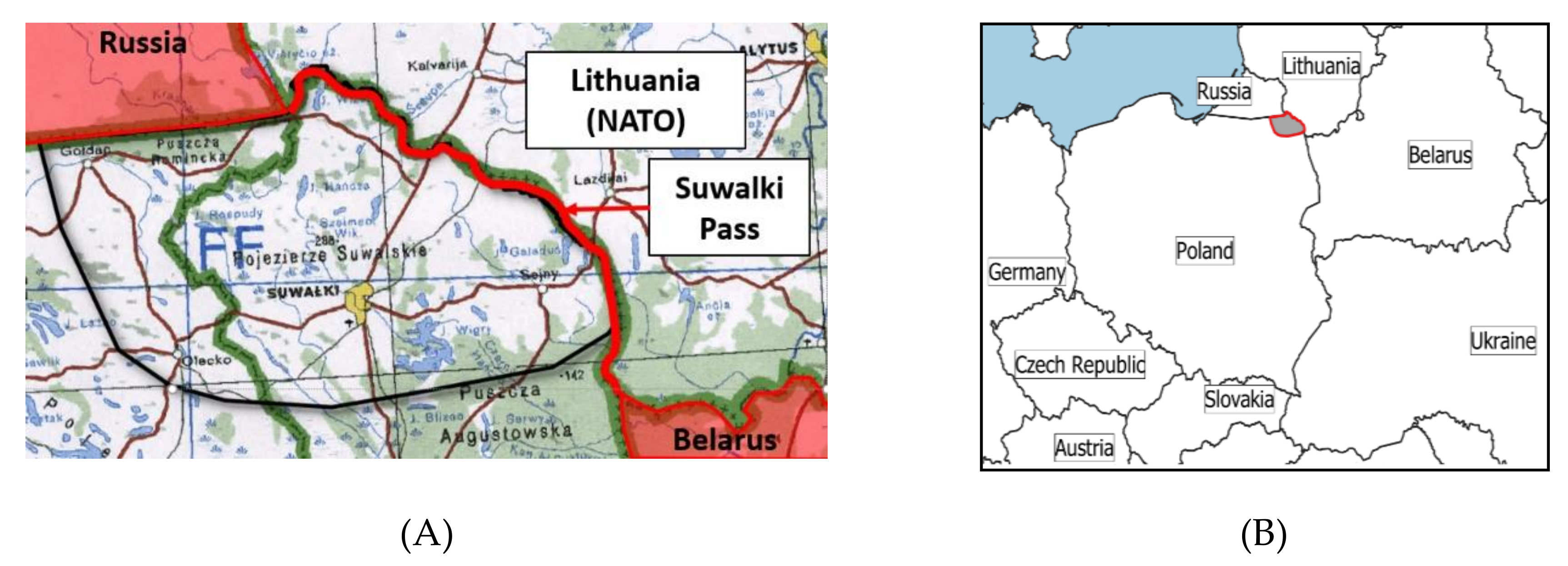
The experiments were conducted for the area of northeastern Poland (Figure 1). From the military point of view, this is an area of key geopolitical importance both for Poland and for the NATO as a whole. In the literature [30], it is often referred to as the Suwałki Pass. It is situated near the Polish–Lithuanian border and covers an area of approximately 3000 km2. Apart from its great strategic importance resulting from the fact that the borders of Poland, Lithuania, Belarus, and Russia meet at one point, the area is characterized by varied land cover. What is important from the crisis management point of view is the fact that it contains large forest areas (approximately 15% of the surface area), some of the largest lakes in Poland (5%), a well-developed river network, and marshes. Its northern part covers both large terrain denivelations (up to 10 degrees) and large, open plains that constitute good passability terrain, as well as a large, developed area (the city Suwałki). As a result of this diversity, the tested area contains terrain of various degrees of passability, which makes it particularly suitable as a representative research site.
2.2. Used Data
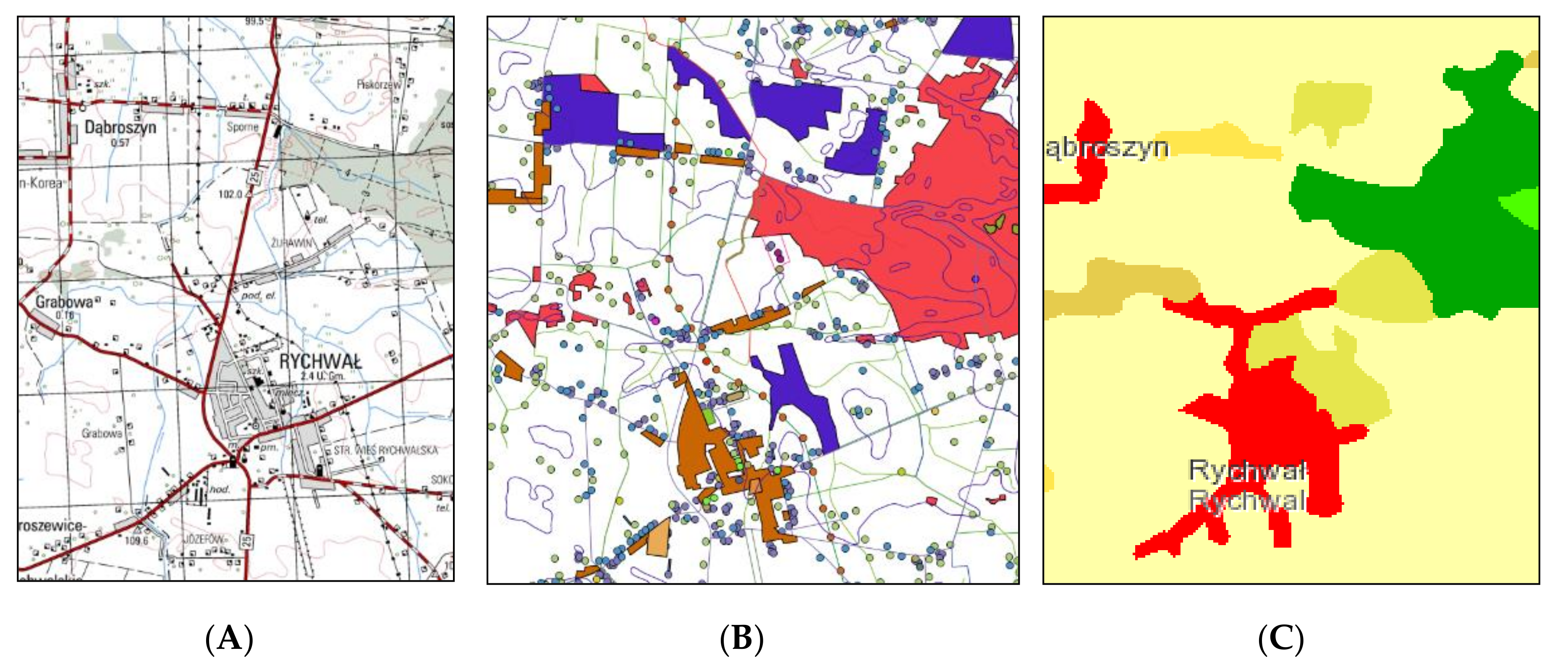
Two sources of spatial data were used as source material, which was the basis for developing passability maps. The first and mainly used one was Vector Map Level 2 (VML2), which is a standard, military, general geographic spatial database of a level of detail corresponding to military topographic maps in a scale of 1:50,000 (Figure 2B). This map covers nine usable object categories, such as borders, relief, physiography, transport, buildings, hydrography, vegetation, and aviation content. The structure of this database is compliant with the DIGEST standard (Digital Geographic Information Exchange Standard) [31] that specifies the method of defining objects for all military vector spatial databases. This database covers the whole territory of Poland. Due to its high level of detail, its authors decided not to expand it to cover the whole area of the NATO alliance. It is the natural, primary, and official source of data for creating passability maps, which is also used as source data to generate other spatial analyses used for military purposes and in crisis management.
The research also used data from Corine Land Cover (for preliminary terrain classification based on land cover elements) (CLC, Figure 2C). This database contains information about land cover (land use) throughout the territory of Europe. It is prepared regularly (usually every 6 years) and also contains information about the changes that occurred between subsequent cycles. The database contains only surface objects grouped in the following classes: anthropogenic areas, agricultural land, wetlands, and aquatic areas. The unit responsible for the coordination of CLC projects on the European level (since the CLC 2000 project) is the European Environment Agency (EEA). The research was based on the newest version of CLC data of the year 2012 [32].
2.3. Method
The basic methodological assumption for the conducted research was to divide the test area into fragments of various sizes. As a result, it was divided into sections called primary fields. For the purposes of the study, these primary fields were either Voronoi polygons (whose method of generation will be described in further sections of the paper) or regular (square) primary fields. The main objective was for maps to be generated in a completely automated way, so a special IT system dedicated for this purpose was created. The system uses vector spatial databases, which are placed in the PostgreSQL relational database with the PostGIS extension. The system carries out all stages of the passability maps development—from counting objects in the square cells through generating primary fields (square and Voronoi polygons) and ending with calculating the passability coefficient for them and visualizing the resulting maps. After the system was configured, it enabled generating various configurations of maps in a completely automated way. Its detailed description is presented in [33].
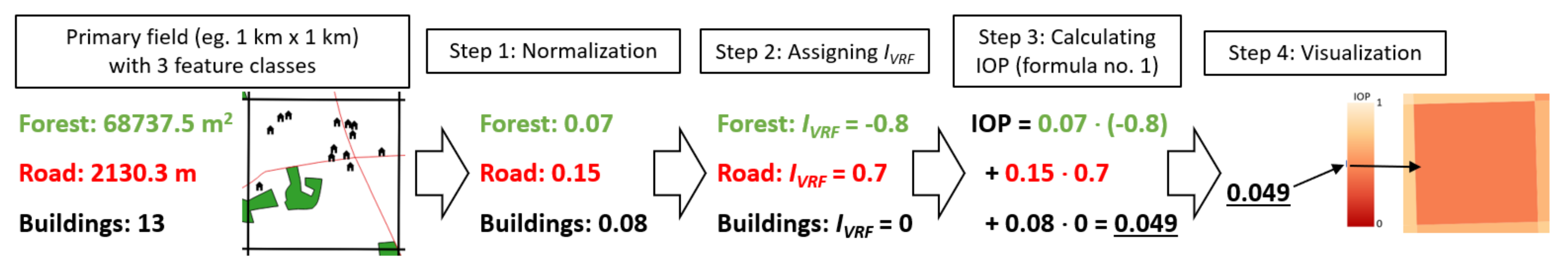
Each primary field was assigned a determined index of passability, which is an estimator that reflects the degree of limiting the movement speed of vehicles while crossing terrain of various land cover, both on roads and off-road, in any weather conditions. It was determined with use of the method developed by the author, hereinafter referred to as the Vegetation Roughness Factor (VRF).
In the discussed method, assume that the IOP (Index of Passability) value would be determined based on the Vegetation Roughness Factor (VRF, denoted as IVRF). VRF is a numerical evaluation reflecting the degree of the speed limit related to the movement of vehicles through different types of land cover. This factor has been determined in a continuous range. The author proposed an algorithm of calculating the index of passability based on the VRF method, which is as follows:
- Land cover data for each primary field (e.g., areas of forests, length of roads, number of buildings, etc.) are normalized to the range from 0 to 1.
- The VRF coefficient is arbitrarily assigned to each category of objects based of [6]. In order to do so, object classes were selected (Table 1) that hinder passability (IVRF < 0), facilitate it (IVRF > 0), and do not affect passability (mainly point objects, IVRF = 0). The analysis parameters may be modified freely by the user defining their own VRF coefficients, which makes the method universal.
- The index of passability is calculated with use of equation:
where
- ○
- is the index of passability of the primary field i,
- ○
- for surface objects, is the normalized surface (located inside the primary field i) of objects from the n1 thematic category,
- ○
- for linear objects, is the normalized length (located inside the primary field i) of objects from the n2 thematic category,
- ○
- for point objects, is the normalized number (located inside the primary field i) of objects from the n3 thematic category,
- ○
- is the vegetation roughness factor for object classes n1, n2, and n3.
Equation (1) takes into account all classes of objects contained in the spatial database. It is possible to exclude a given class from the analysis by removing it through assigning it an of 0 (not affecting passability). In the presented research, information from all feature classes included in VML2 was introduced into Formula (1). However, it should be emphasized that the presented methodology also allows taking into account data from other databases, enriching the analysis with information on the impact of soils, weather conditions, etc.
A schematic presentation of the operation of the algorithm is presented in Figure 3.
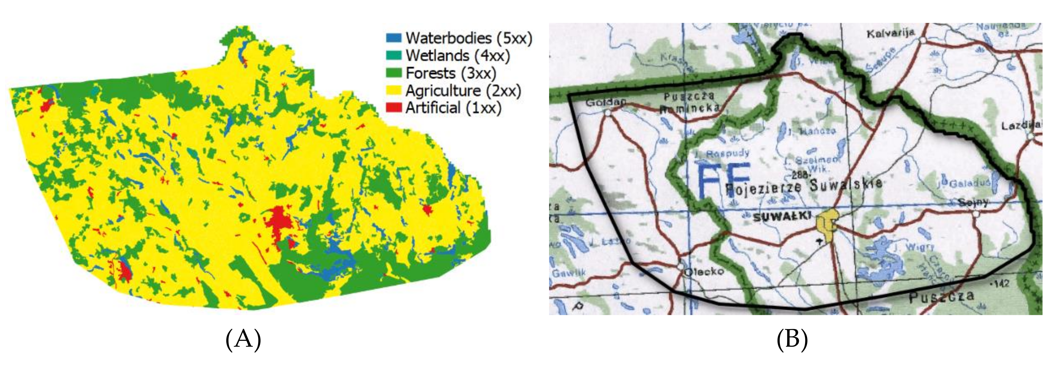
Variable resolution maps were generated in two configurations. The first method was based on the application of regular (square) primary fields of varied sizes. The objective of the method was to cover the areas of more complex land cover structure in terms of passability with square primary fields of a smaller size. The decision of which parts of the area should be covered with smaller primary fields (as smaller primary fields enable the visualization of a higher level of detail) was made by dividing the tested area into zones whose spatial range depends on the degree of land development. The following algorithm was applied:
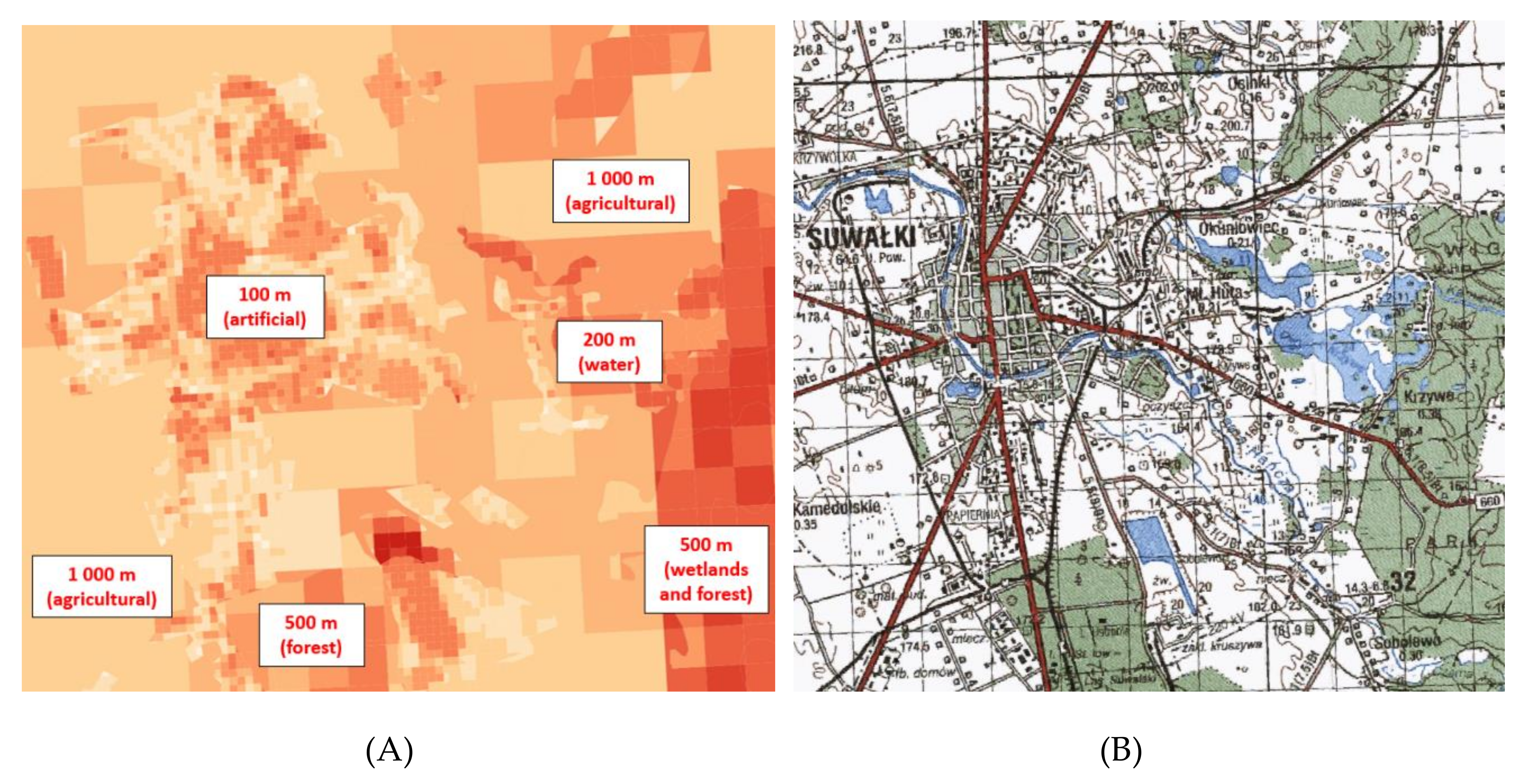
- Each distinguished class of land cover was assigned a passability map consisting of primary fields of a specific size, according to the methodology presented below and in [33]. It was assumed that areas characterized by a complex land cover structure would be presented with the use of smaller primary fields (100 m squares, e.g., built-up areas), while larger primary fields (e.g., 1000 m squares) would be used for less varied areas (e.g., arable land, see Table 2).
- A fragment of the mosaic created in this way is presented in Figure 5.
The second method of creating variable resolution passability maps was based on the application of irregular primary fields of various sizes. The algorithm for dividing the test area into fragments was as follows:
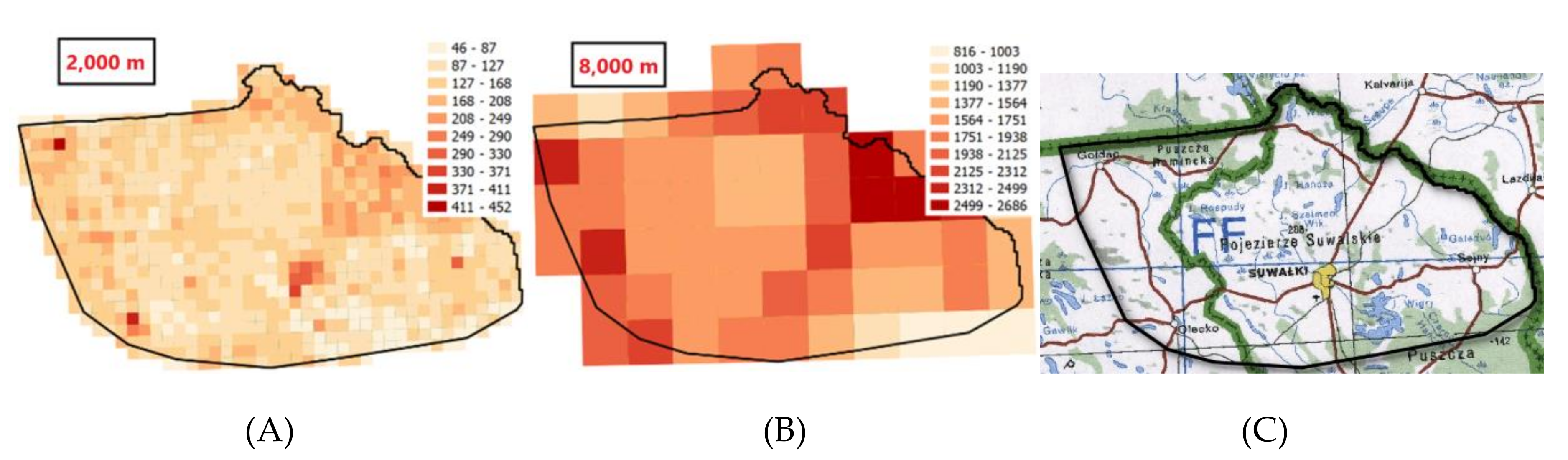
- The test area was divided into regular, square primary fields. Tests were conducted for 2000 m and 8000 m squares (Figure 6).
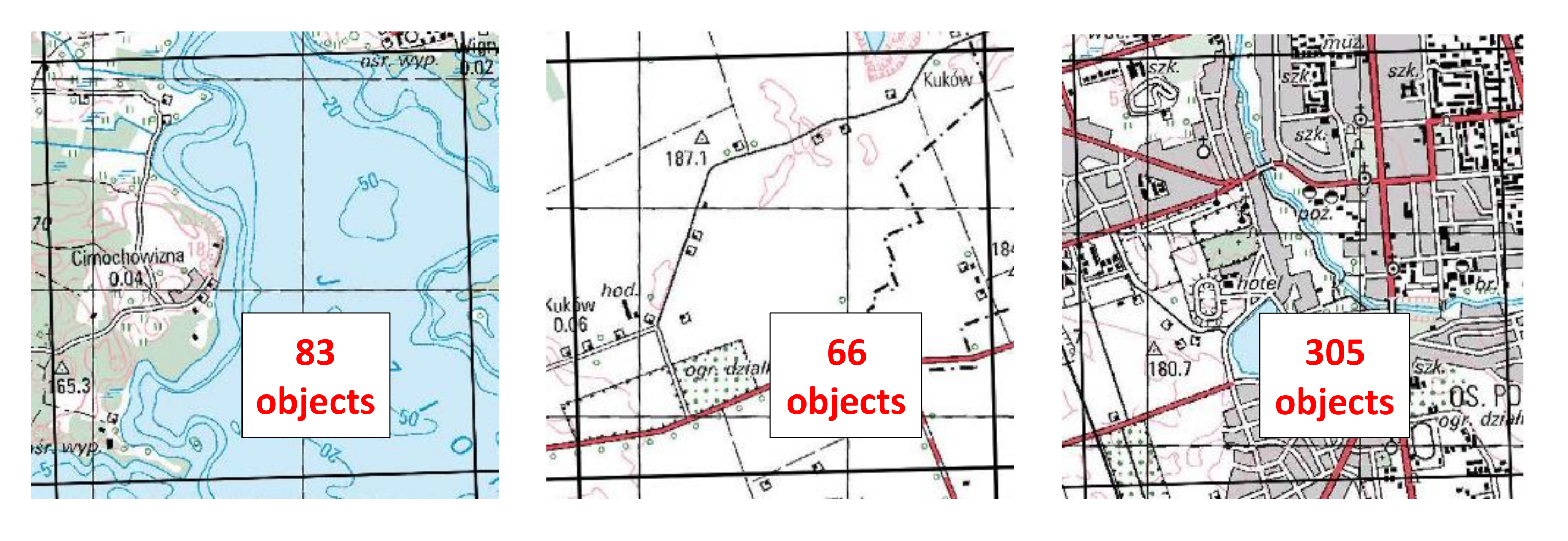
- The IT system determines the number of objects that exist inside each primary field (Vector Map Level 2 was used for this purpose). The results of this operation are presented in Figure 6. Adopting this assumption allowed us to distinguish areas characterized by complex land cover in the map. It was assumed that the land cover structure in squares that contain a small number of spatial objects is weakly diversified, which is confirmed by the examples shown in Figure 7.
- Depending on the number of objects in the given primary field, the system places points randomly inside these fields (the more objects that exist inside a given field, the more points are generated inside it). The number of points was determined proportionally to the number of all objects inside the given square. The developed IT system allows selecting the minimum and maximum number of points generated in each square. It also allows the determination of a percentage of the number of points, below which points in the given field will not be generated at all (threshold). It was determined with use of the formula developed by the author, i.e., if the number of points in the given square is lower than the result of Equation (2), then points in this square will not be generated at all. Table 3 shows how the change in the threshold coefficient influences the points generated on the map.
where
- value—number of points in the square;
- valuemax, valuemin—the fixed maximum and minimum number of points generated in a square;
- threshold—determined value of the threshold coefficient expressed as percentage.
The application of the above relation and determining the appropriate “threshold” percentage allowed us to generate points only in the area with the most diverse land relief and development types. As Table 3 clearly demonstrates, this has a major influence on the information content of the map and the number of generated points (and thus of the primary fields).
- 4.
- Then, the obtained points constitute the basis for generating primary fields in form of Voronoi polygons (called also a Voronoi diagram, see Table 4). The Voronoi diagram is a division of the area into regions close to each of a given set of objects. In the simplest case, these objects are just a finite number of points in the plane (called seeds, sites, generators, or just points). For each seed, there is a corresponding region consisting of all points of the plane closer to that seed than to any other. These regions are called Voronoi cells (or polygons). These polygons are often used to determine the areas that may be treated as “served by” (or closest to) the given point. In the presented research, they were generated based on Euclidean distance. These polygons are commonly used for the tessellation of areas in numerous practical applications, including indoor localization [34], spatial economic analyses (e.g., for determining the location and range of impact of shops [35]) or in biological studies [36]. A detailed algorithm for generating these objects was presented in [37].
- 5.
- Then, the index of passability, being an estimate reflecting the degree of limitation of vehicular speed by land cover elements, is determined for each Voronoi field. The IOP is calculated based on the parameters related to land cover and terrain formation elements that exist in in the given primary field (Voronoi polygon). The index of passability was determined with use of the methodology presented above and in [33].
Then, using the presented method, generated maps with the use of various combinations of shapes and sizes of generated Voronoi primary fields were subjected to comparisons, both between each other and with maps of passability described in [9] created using square primary fields in various sizes.
3. Results
Various configurations of passability maps were generated.
- Two sizes of squares (2 km and 8 km) were used, in which objects from VML2 were counted.
- For each of these square sizes, Voronoi polygons were generated, which were then assigned indices of passability. The Voronoi polygons were generated:
- ○
- For the maximum number of points in a square equal to 10, 30, and 50 points.
- ○
- For maps generated based on the assumption that a field could contain a maximum of 30 points, changes in the threshold coefficient were analyzed. Tests were conducted for the coefficient of 0%, 25%, and 50% of the points.
- ○
- For maps generated based on the assumption that a field could contain a maximum of 50 points, the changes in the minimum number of points generated in each field were tested. The analyzed minimum number of points equaled 0, 20, and 40 pts.
In order to prepare a discussion and draw conclusions, statistical analyses were performed for each obtained map. These analyses consisted of:
- Calculating the statistics both for the distribution of the surface area of the generated primary fields and for the obtained indices of passability. The following were calculated: Average value (Av), standard deviation (Std.), median (Med.), skew (Skew.), and kurtosis (Kurt.), as well as the total number of generated fields (Qty.).
- Calculating the histograms of the distribution of the surface area for the generated primary fields and the histograms of the distribution of the obtained indices of passability.
Additionally, each generated map was visualized cartographically with use of the cartogram method. In order to improve the possibilities to analyze the distribution of the obtained primary fields for each map, the area located in the proximity of the city of Suwałki was enlarged. The results described above are presented in Table 5 and Table 6.
Maps created from the Voronoi polygons were compared with those generated with the use of regular, square primary fields of various sizes, whose visualizations and statistics are presented in Table 7.
In order to compare the content of generated maps, the grid (in size 500 by 500 m) of control points was placed in the test area. Each of these points included obtained data about the value of passability where the given control point was located. This operation was performed for all generated maps. Thus, each control point was assigned 14 indices of passability. Based on this huge table of indices of passability, Pearson correlation matrices (presented in Table 8) were calculated. Matrices were determined for all the generated maps of passability (generated using Voronoi polygons in various configurations and regular primary fields in sizes 100 × 100 m, 200 × 200 m, 500 × 500 m, 1 × 1 km, 2 × 2 km, and 5 × 5 km). The results of these calculations are presented in Table 8.
4. Discussion
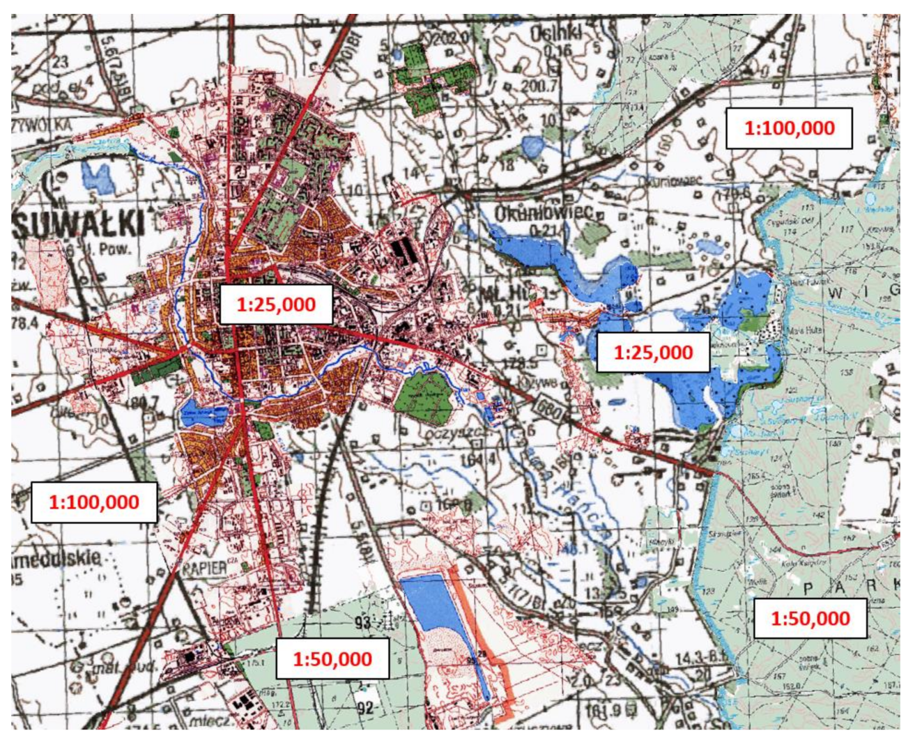
In the initial stage of research on variable resolution maps, the author conducted a very simple experiment that consisted of creating such a map from a mosaic of raster maps in various scales. Such a map may be created easily by dividing the area into classes and assigning them a raster map in the relevant scale. The result of such an experiment is presented in Figure 8. The division into areas was consistent with CLC, while the scales of maps were selected according to the objectives presented in Table 2. The obtained map is doubtlessly interesting from the graphic point of view, but it is quite difficult to use due to different levels of generalization, which is directly linked to the application of various scales (as it was discussed in Section 1). As a result of the discrepancies in the selection of content, maps in different scales also use different conventional signs that often differ in terms of both symbols and size.
A similar approach was adopted while creating passability maps of variable resolution with use of square primary fields of different sizes, depending on the covered area (Figure 5). As a result of this operation, a map consisting of a total of 20,770 primary fields was created. This value accounts for only 7% of the number of square primary fields of the size of 100 × 100 m covering the tested area and 28% of the number of 200 × 200 m square primary fields. It should be noted that the obtained result of nearly 21 thousand primary fields is an equivalent of covering the tested area with identical square primary fields of the size of approximately 380 m. This results from the fact that areas where large primary fields were applied account for approximately 95% of the tested area. The application of large primary fields in these areas was justified, as they were characterized by simple land cover structure, without a large number of terrain details. On the other hand, urban areas, which require a much more detailed presentation, occupy only 2% of the whole test area. An advantage of the applied method is a noticeable reduction in the total amount of data (primary fields) stored in the database while, at the same time, maintaining a detailed representation of selected areas that are important from the point of view of passability (mainly urban areas). The remaining areas (e.g., agricultural and wooded areas and waters) were presented in a less detailed way due to their monotonous and undiversified passability conditions. Although the proposed map was generated with the use of square primary fields, they were fitted into areas with various land cover types, so the square fields were cropped at the edges, resulting in the emergence of figures of various, usually irregular shapes (Figure 5). The presence of these discontinuities (sudden changes in the detail level of individual areas) may hinder the practical use of the map by users. These disadvantages do not exist in the maps generated with the use of a method based on the Voronoi polygons. Their use makes the structure of the map consistent, and the change of detail level does not occur suddenly, making the map continuous and homogeneous in terms of the shapes of used primary fields. In addition, this method allows for the precise definition of areas with variable information density (especially when using small squares in which spatial database objects are counted e.g., 2 × 2 km). In the case of method no. 1, which is based on square primary fields of various sizes, the distinction between areas with a specific detail depends on the number of classes used. In this study, there were only five classes chosen from the Corine Land Cover database.
The second method of generating primary fields, based on Voronoi polygons and developed by the author, was subjected to separate, very detailed analyses. It is worth noting that all the obtained and analysed maps were created based on the same data and with use of the same method of calculating the index of passability. Maps were created only by changing (modifying) the parameters of the process of generating primary fields, which means that the obtained results depended only on these parameters.
4.1. Change in the Size of the Average Primary Field Depending on the Assumed Parameters
The analysis of the average size of the generated primary fields (Figure 9) revealed that increasing the maximum number of points in a square resulted in a linear decrease in their size (the blue line in the diagrams). The average size of the primary field ranged from 1.9 km2 for a maximum of 10 points in a 2 × 2 km square to 0.4 km2 for 50 points. If larger squares are used (8 × 8 km), the generated fields are bigger, which is caused by the fact that the total number of points placed in the test area is lower. The average fields for this square range from over 11 km2 for 10 points per square to 2.4 km2 for 50 points. The significant increase in the surface area of the generated primary fields is noticeable when the threshold coefficient for points generated in square fields is increased (the orange line in the diagram). For 2 × 2 km2, at the threshold coefficient of 50% (as a reminder: the threshold coefficient is the percentage of the number of points below which Voronoi polygons will not be generated at all for the given square), the average size of the obtained fields reached almost 30 km2. When larger squares were used, this increase was less dramatic, and for a 50% threshold, the average field size was nearly 11 km2 (without any threshold, the size of the average field was 4 km2). The change in the value of the third parameter, which is the determination of the maximum number of points in the square, always led to the increase in the number of generated Voronoi polygons and a decrease in their average size (gray line in the diagram). For 2 × 2 km2, when 40 to 50 points were generated in each field, the size of the average field was only 0.1 km2.
4.2. Change in the Standard Deviation of the Surface Area of Generated Primary Fields
The standard deviation of the primary field surface area was calculated for each map. This should be interpreted as a measure of the spread of the surface areas of primary fields. A high value of the standard deviation indicates that the map contains both very large and very small primary fields at the same time. The analysis of the diagrams presented in Figure 10 demonstrates clearly that their characteristics correspond to the correlations presented in Figure 9 that refer to the average size of the field. The aim of the method was to ensure that the map would contain different sizes of primary fields, so the values of the standard deviation are relatively high in nearly all cases. For maps where no minimum number of points or threshold coefficient was applied (blue line in the diagram), the value of standard deviation is approximately equal to the average field surface, and it decreases with the increase in the maximum number of points in the square. This is caused by the growing number of emerging Voronoi polygons. The application of the threshold coefficient (orange line in the diagram) leads to a significant, dramatic surge in the standard deviation, which is manifested in the emergence of very large primary fields in areas with less diversified land cover and very small fields in highly developed areas. Reverse results are obtained by increasing the minimum number of points in the square (gray line in the diagram). Then, the sizes of primary fields become similar, which is reflected in the low value of the standard deviation of primary field surface area.
4.3. Change in the Number of Generated Primary Fields
The main aim of the research was to develop a method to decrease the number of primary fields covering a pre-defined area while maintaining possibly high informational content of the generated map. The correlations presented in Figure 11 demonstrate clearly that increasing the maximum number of points in a square results in generating a higher number of Voronoi polygons (blue line in the diagrams). For a 2 × 2 km square with a maximum of 10 points, 1766 polygons are obtained, while the number of polygons reaches 8783 if the maximum number of points is increased to 50. One way to reduce the number of polygons is to increase the size of squares in which points are generated. Thus, for an 8 × 8 km square with a maximum of 10 points, only 294 polygons are obtained, and for a maximum of 50 points, there are 1436. As the diagrams show, another very effective way to reduce the number of primary fields is to consider a threshold coefficient (orange line in the diagram). In the conducted analyses, for a 2 × 2 km square, increasing this coefficient to 25% leads to a nearly six-fold decrease in the number of fields (896 fields), while setting the coefficient to 50% allows reducing it 46 times (114 fields) in comparison to maps generated without this estimator (5274 fields). Completely reverse results are obtained by increasing the minimum number of points in the square (gray line in the diagram). Here, setting the minimum number of points to 20 for a 2 × 2 km square increases the number of generated fields 2.4 times (21,314 fields), and if the value of the coefficient increases to 40, the number of fields grows 3.8 times (33,825 fields). For comparison, the number of fields obtained without setting the minimum number of points is 8783.
4.4. Change in the Average Value of the Index of Passability
The main task of the generated maps is to present the index of passability correctly. Figure 12 presents the changes in the average value of IOP depending on the selected configuration of input parameters. The diagrams show that changes in the maximum number of points per square (blue line) have only a slight influence on the average value of the IOP. On the other hand, it increases visibly when a threshold coefficient is applied (orange line), and it is caused by the decreased level of detail of the created passability maps. Each Voronoi polygon contains numerous objects that have both a positive and negative influence on passability, which “moves” the average IOP toward higher values. The application of a minimum number of points per square increases the detailedness of the map and provides a better representation of separated impassable areas so that the average value of IOP is lower (gray line in the diagram).
4.5. Comparison of the Correlation Coefficients between Passability Maps
The calculated correlation coefficients are a measure of the similarity of the resulting passability maps. They are used to compare the spatial distribution of indices of passability. The analysis of the obtained matrix of correlations (Table 8) allows us to claim that the obtained maps are generally similar, as the average value of all correlation coefficients is as high as 0.75. The aim of the analysis of the correlation matrix was to find the highest coefficients of correlation with the map with the largest information content. This is the map based on 100 × 100 m square primary fields, which consists of almost 300 thousand such fields. It turned out that the maps that are marked with frame 1 in Table 8 have the highest coefficient of correlation with this map. An exception is the map generated based on 2 × 2 km2, where a maximum of 50 points was placed. It consists of nearly 34 times fewer primary fields than the map created from 100 × 100 m squares, but the correlation coefficient between these maps is very high, and it amounts to 0.80 (Table 9, Example 1). As for the comparison of maps based on larger square primary fields (e.g., 1000 × 1000 m), the highest correlation coefficients were calculated for maps generated with use of primary 8 × 8 km2 (Table 8, Frame 2). Here, again, the highest correlation coefficients were found for the map created with use of a maximum of 50 points. The use of the best configuration allows reducing the number of primary fields at least by half (1436 fields in the map based on Voronoi polygons versus 3084 square primary fields 1 by 1 km, at the correlation coefficient of 0.81, Table 9, Example 2). The correlation matrix also enables us to find very high correlation coefficients between the maps generated with use of Voronoi polygons. The examples presented in Table 3 and Frame 3 are particularly noteworthy. They show very high correlation coefficients between maps that consisted of very different numbers of primary fields (e.g., Table 9, Example 3).
5. Summary
The paper presents methods of generating variable resolution passability maps. The author propose methodologies that enable the automated creation of such maps, taking into account the density of terrain objects covering the area. Referring to the research questions contained in Section 1.2, the author presented (in Section 2) two methods that allow for the generation of variable-resolution accessibility maps. Importantly, they are prone to the automation process, which is clearly proven by the fact that the author has prepared an application in the .NET environment, which automatically generates them using the presented methods. The methodologies, thanks to the use of the Corine Land Cover database (method No. 1) or the number of spatial database objects (VML2, method 2) in a defined area (in the case of the conducted research, it was a square with a side of 2 km and 8 km), allow the diversity of the analyzed area due to the density of its cover elements. It was necessary to generate variable resolution maps of terrain passability. The analyses were conducted assuming specific and user-defined parameters. Their influence on the resulting maps is included in the “Discussion” section; the following sections (4.1–4.4) analyze the influence of defined input parameters on the obtained resulting passability maps.
Apart from the presented “mosaic” of raster maps in various scales, which seems interesting from the graphic point of view, but difficult to use, the first method was based on the application of square primary fields of various sizes. The application of his method allows for a significant reduction of the number of primary fields constituting the map. This results from the fact that areas where large primary fields were applied account for approximately 95% of the tested area. The application of large primary fields in these areas was justified, as they were characterized by simple land cover structure without a large number of terrain details. On the other hand, urban areas, which require a much more detailed presentation, occupy only 2% of the whole test area. The generated map consists of a total of over 27 thousand primary fields of various sizes.
The second method consisted in using Voronoi polygons. It was demonstrated that the method enables generating these polygons based on various configurations of input parameters. In this aspect, it is completely universal, which is proven by Figure 13 (left side). The map was generated based on the assumption that 10 points were randomly placed in the surface area of a square of a side length of 5 km. The number of points placed in the remaining fields was determined based on the proportional extrapolation of the number of objects from VML2. These points constituted the basis for creating Voronoi polygons. Then, the obtained map was compared with the map consisting of square primary fields of a side length of 1 km (Figure 13, right side).
Using both methods, maps can be developed automatically; therefore, the selection of the appropriate method depends on the requirements and preferences of the users who will use the map.
It should be emphasized that the proposed methodologies are very susceptible to modification, an example of which is that the points on the basis of which Voronoi polygons are created can be located not only on the basis of the number of all objects contained in the spatial database. Depending on the nature of the presented phenomenon, any type of them (e.g., surface, line, point) or only one or several classes of objects (e.g., number of roads, buildings, etc.) can be taken into account.
The comparison consisted of placing control points on both maps, in a 0.5 by 0.5 km grid, and reading the indices of passability for them. The resulting Pearson’s coefficient between indices of passability read from the map was 0.87, which proves that the degree of similarity between the two compared maps was very high. Such high correlation allows us to conclude that the informational content of both maps is very similar. This conclusion is even more important considering that the map created with use of irregular primary fields consisted of 1076 such fields, while the number of fields in the map generated with the use of regular squares was nearly three times higher: 3084. This leads to a very important conclusion: the application of the method of creating irregular primary fields presented in our study allows the reduction of the number of primary fields while at the same time maintaining a high informational content of the resulting map. This is confirmed by the distribution of primary field sizes, which demonstrates that the most fields on the generated map have a size of approximately 1 km2 and the average field surface size is 3 km2. The distribution also reveals a high number of primary fields smaller than 1 km2, which were placed in the area containing the highest number of objects (mainly urban areas) and fields of a larger surface located mainly in forests and arable lands.
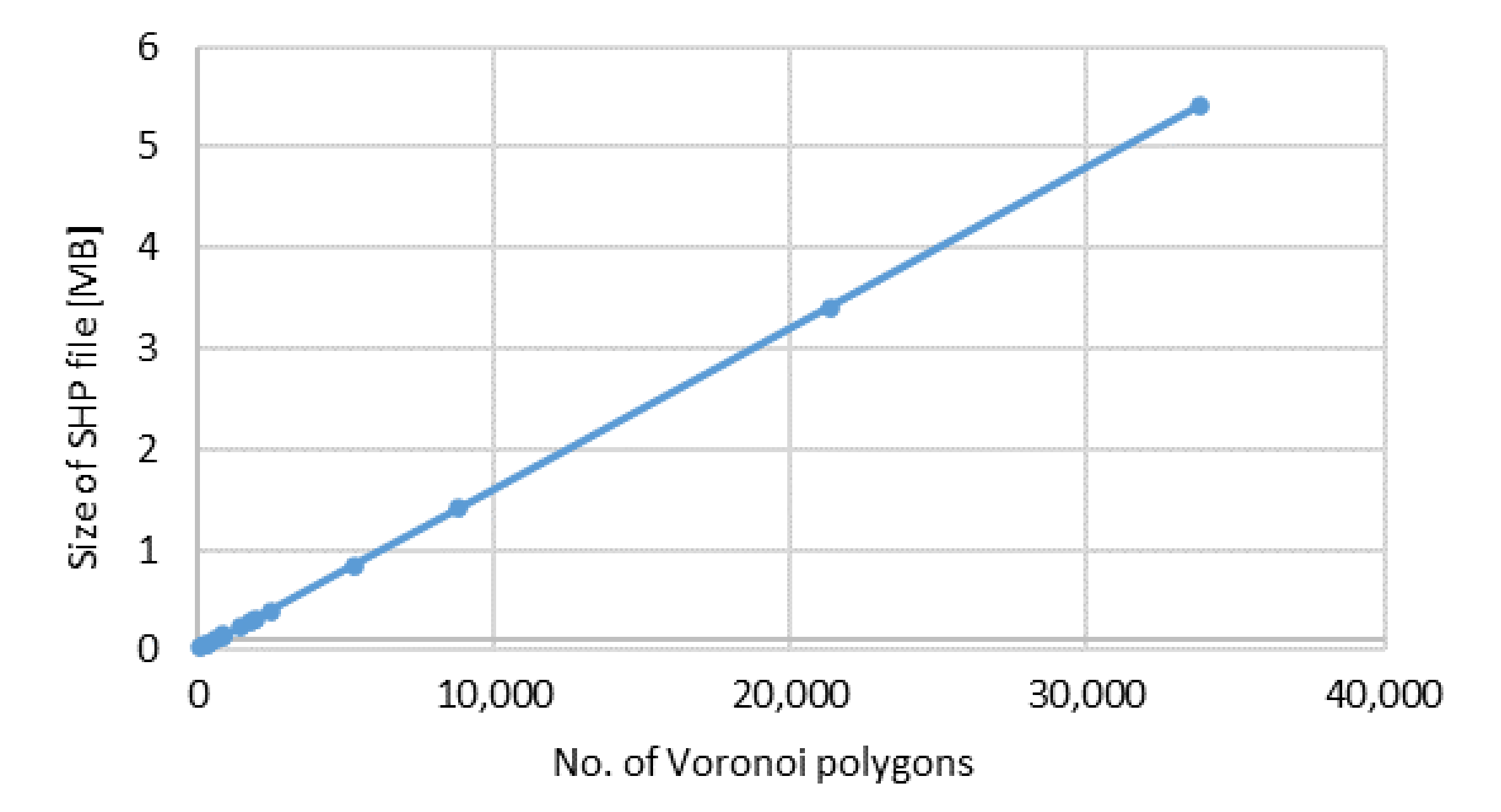
The research conducted so far has revealed that the automated generation of passability maps with the use of various sizes of primary fields is possible. The application of such primary fields offers numerous tangible benefits. First of all, it enables reducing the number of fields covering the given area without limiting the usability and level of detail of the map. It is important from the point of view of the time required to create such a map. Additionally, it has a positive influence on the usefulness of the map, as it allows users to focus on the most important terrain features. This has an enormous practical value and allows users to answer the next research question contained in Section 1.2, relating to the use of the generated maps. This has an enormous practical value for potential users who are not professional cartographers (commanders, leaders of search and rescue operations), as the reduction of the number of primary fields has an important and certainly practical aspect: it allows saving a great amount of space in the computer memory where these data are stored. This correlation is presented in Table 10, where the space occupied in computer memory by shp files containing only the geometry of Voronoi polygons.
Figure 14 reveals that the file size is proportional to the number of primary fields creating the map. Considering the high correlation coefficients between the obtained maps (Table 8), one may find such parameters that will enable creating a map characterized both by high information content and by a small size of occupied memory.
As far as the test area described in the paper is concerned, the space occupied on a disk by all passability maps is small and insignificant. However, if we collect data for the territory of the whole country or even a continent, then using variable resolution data may significantly accelerate their use and at the same time save valuable space in computer memory.
Funding
The research was funded by the Military University of Technology in Warsaw, Poland under the University Research Grant, grant number 793/2020, realized in year 2020.
Acknowledgments
This research was performed on the basis of Vector Map Level 2 obtained from Polish Military Directorate.
Conflicts of Interest
The authors declare no conflict of interest.
References
- Ware, J.M.; Jones, C.B.; Thomas, N. Automated map generalization with multiple operators: A simulated annealing approach. Int. J. Geogr. Inf. Sci. 2003, 17, 743–769. [Google Scholar] [CrossRef]
- Viaña, R.; Magillo, P.; Puppo, E.; Ramos, P.A. Multi-VMap: A Multi-Scale Model for Vector Maps. Geoinformatica 2006, 10, 359–394. [Google Scholar] [CrossRef]
- Weibel, R.; Burghardt, D. Generalization, On-the-Fly. In Encyclopedia of GIS; Shekhar, S., Xiong, H., Eds.; Springer: Boston, MA, USA, 2008; pp. 339–344. ISBN 978-0-387-35973-1. [Google Scholar]
- Google Maps. Available online: https://www.google.com/maps/ (accessed on 10 September 2020).
- OpenStreetMap. Available online: https://www.openstreetmap.org/ (accessed on 10 September 2020).
- NO-06-A015:2012 (Ed.) Terrain—Rules of Classification—Terrain Analysis on Operational Level; (Teren - zasady klasyfikacji - ocena terenu na szczeblu operacyjnym); Ministry of National Defence: Warsaw, Poland, 2012. [Google Scholar]
- Defence standard STANAG 3992, ed. 2: Military Geographic Documentation—Terrain Analysis AgeoP-1 (A). 1999.
- Military Specification MIL-V-89032 Vector Smart Map (VMAP) Level 2. 1993.
- Pokonieczny, K.; Mościcka, A. The Influence of the Shape and Size of the Cell on Developing Military Passability Maps. ISPRS Int. J. Geo-Inf. 2018, 7, 261. [Google Scholar] [CrossRef] [Green Version]
- Hofmann, A.; Hošková-Mayerová, Š.; Talhofer, V.; Kovařík, V. Creation of models for calculation of coefficients of terrain passability. Qual. Quant. 2015, 49, 1679–1691. [Google Scholar] [CrossRef]
- Pokonieczny, K.; Rybansky, M. Method of developing the maps of passability for unmanned ground vehicles. IOP Conf. Ser. Earth Environ. Sci. 2018, 169, 012027. [Google Scholar] [CrossRef] [Green Version]
- Dohnal, F.; Hubacek, M.; Simkova, K. Detection of Microrelief Objects to Impede the Movement of Vehicles in Terrain. ISPRS Int. J. Geo-Inf. 2019, 8, 101. [Google Scholar] [CrossRef] [Green Version]
- Hubáček, M.; Almášiová, L.; Dejmal, K.; Mertová, E. Combining Different Data Types for Evaluation of the Soils Passability; Ivan, I., Singleton, A., Horák, J., Inspektor, T., Eds.; Springer International Publishing: Cham, Switzerland, 2017; pp. 69–84. [Google Scholar]
- Rybansky, M. Soil trafficability analysis. In Proceedings of the International Conference on Military Technologies (ICMT), Brno, Czech Republic, 19–21 May 2015; pp. 1–5. [Google Scholar]
- Sun, H.; Li, Z. Effectiveness of Cartogram for the Representation of Spatial Data. Cartogr. J. 2010, 47, 12–21. [Google Scholar] [CrossRef]
- Batista e Silva, F.; Gallego, J.; Lavalle, C. A high-resolution population grid map for Europe. J. Maps 2013, 9, 16–28. [Google Scholar] [CrossRef]
- Calka, B.; Bielecka, E. Reliability Analysis of LandScan Gridded Population Data. The Case Study of Poland. ISPRS Int. J. Geo-Inf. 2019, 8, 222. [Google Scholar] [CrossRef] [Green Version]
- Zhang, H.; Chen, Y.; Gao, P.; Wu, Z. Mapping the changing Internet attention to the spread of coronavirus disease 2019 in China. Environ. Plan A 2020, 52, 691–694. [Google Scholar] [CrossRef]
- Markowska, A.; Korycka-Skorupa, J. An evaluation of GIS tools for generating area cartograms. Pol. Cartogr. Rev. 2015, 47, 19–29. [Google Scholar] [CrossRef] [Green Version]
- Sun, S. Applying forces to generate cartograms: A fast and flexible transformation framework. Cartogr. Geogr. Inf. Sci. 2020, 47, 381–399. [Google Scholar] [CrossRef]
- Pokonieczny, K. Methodology of cartographic visualisation of military maps of passability. In Proceedings of the 7th International Conference on Cartography and GIS, Sozopol, Bulgaria, 18–23 June 2018; pp. 613–622. [Google Scholar]
- Pokonieczny, K. Comparison of land passability maps created with use of different spatial data bases. Geogr. Sb. CGS 2018, 123, 317–352. [Google Scholar] [CrossRef]
- Harrie, L.; Stigmar, H. An evaluation of measures for quantifying map information. ISPRS J. Photogramm. Remote Sens. 2010, 65, 266–274. [Google Scholar] [CrossRef]
- Zaragozí, B.; Giménez, P.; Navarro, J.T.; Dong, P.; Ramón, A. Development of free and opensource GIS software for cartographic generalisation and occupancy area calculations. Ecol. Inform. 2012, 8, 48–54. [Google Scholar] [CrossRef]
- Yu, W.; Zhang, Y.; Chen, Z. Automated Generalization of Facility Points-of-Interest with Service Area Delimitation. IEEE Access 2019, 7, 63921–63935. [Google Scholar] [CrossRef]
- Bayer, T. Estimation of an unknown cartographic projection and its parameters from the map. Geoinformatica 2014, 18, 621–669. [Google Scholar] [CrossRef]
- Tomono, M. Planning a path for finding targets under spatial uncertainties using a weighted Voronoi graph and visibility measure. In Proceedings of the 2003 IEEE/RSJ International Conference on Intelligent Robots and Systems (IROS 2003), (Cat. No.03CH37453). Las Vegas, NV, USA, 7 January 2004; Volume 1, pp. 124–129. [Google Scholar]
- Melkemi, M.; Hammoudi, K. Voronoi-based image representation applied to binary visual cryptography. Signal Process. Image Commun. 2020, 87, 115913. [Google Scholar] [CrossRef]
- Pokonieczny, K. Methods of Using Self-organising Maps for Terrain Classification, Using an Example of Developing a Military Passability Map. In Proceedings of the Dynamics in GIscience, Ostrava, Czech Republic, 22–24 March 2017; Springer: Cham, Switzerland, 2017; pp. 359–371. [Google Scholar]
- Elak, L.; Śliwa, Z. The Suwalki gap—NATO’s fragile hot spot. Zesz. Nauk. AON 2016, 103, 24–40. [Google Scholar]
- Defence standard STANAG 7074, ed. 2: Digital Geographic Information Exchange Standard (DIGEST). 1998.
- CORINE Land Cover—Copernicus Land Monitoring Service. Available online: http://land.copernicus.eu/pan-european/corine-land-cover (accessed on 1 October 2017).
- Pokonieczny, K. Automatic military passability map generation system. In Proceedings of the 2017 International Conference on Military Technologies (ICMT), Brno, Czech Republic, 31 May–2 June 2017; pp. 285–292. [Google Scholar]
- Arif, M.; Wyne, S.; Nawaz, S.J. Indoor localization using Voronoi tessellation. Adv. Electr. Comput. Eng. 2018, 18, 85–90. [Google Scholar]
- Lai, W.-H.; Hung, K.-Z. Optimizing new chain retail store area by using Voronoi diagram technique. In Proceedings of the Picmet 2010 Technology Management for Global Economic Growth, Pukhet, Thailand, 18–22 July 2010; pp. 1–10. [Google Scholar]
- Kim, D.-S.; Cho, Y.; Kim, D.; Kim, S.; Bhak, J.; Lee, S.-H. Euclidean Voronoi diagrams of 3D spheres and applications to protein structure analysis. Jpn. J. Indust. Appl. Math. 2005, 22, 251. [Google Scholar] [CrossRef]
- Sack, J.R.; Urrutia, J. Handbook of Computational Geometry; Elsevier: Amsterdam, The Netherlands, 1999; ISBN 978-0-08-052968-4. [Google Scholar]
Figure 1.
Tested research area. (A)—course of the Suwalki Pass, (B)—location of the test area on the territory of Poland and neighboring countries.
Figure 1.
Tested research area. (A)—course of the Suwalki Pass, (B)—location of the test area on the territory of Poland and neighboring countries.

Figure 2.
Comparison of the visualization of used data: (A)—topographic map in the scale of 1:50,000, (B)—Vector Map Level 2, (C)—Corine Land Cover 2018.
Figure 2.
Comparison of the visualization of used data: (A)—topographic map in the scale of 1:50,000, (B)—Vector Map Level 2, (C)—Corine Land Cover 2018.

Figure 3.
Visualization of the algorithm determining the IOP for sample data according to the VRF method.
Figure 3.
Visualization of the algorithm determining the IOP for sample data according to the VRF method.

Figure 4.
Visualization of the distinguished classes of Corine Land Cover (A) and its comparison with the content of the map (B).
Figure 4.
Visualization of the distinguished classes of Corine Land Cover (A) and its comparison with the content of the map (B).

Figure 5.
Fragment of map created using different field sizes (A) and its comparison with a map in the scale of 1:100,000 (B).
Figure 5.
Fragment of map created using different field sizes (A) and its comparison with a map in the scale of 1:100,000 (B).

Figure 6.
2000 × 2000 m (A) and 8000 × 8000 m (B) fields with a number of objects and its comparison with the content of the map (C).
Figure 6.
2000 × 2000 m (A) and 8000 × 8000 m (B) fields with a number of objects and its comparison with the content of the map (C).

Figure 7.
Comparison of objects density.

Figure 8.
Fragment of the mosaic of raster maps in various scales.

Figure 9.
Diagrams of the changes in the average surface area for squares: (A)—2 × 2 km, (B)—8 × 8 km.
Figure 9.
Diagrams of the changes in the average surface area for squares: (A)—2 × 2 km, (B)—8 × 8 km.

Figure 10.
Diagrams of the changes in the standard deviation of the primary field surface area for squares: (A)—2 × 2 km, (B)—8 × 8 km.
Figure 10.
Diagrams of the changes in the standard deviation of the primary field surface area for squares: (A)—2 × 2 km, (B)—8 × 8 km.

Figure 11.
Diagrams of changes in the number of generated primary fields for squares: (A)—2 × 2 km, (B)—8 × 8 km.
Figure 11.
Diagrams of changes in the number of generated primary fields for squares: (A)—2 × 2 km, (B)—8 × 8 km.

Figure 12.
Diagrams of the average value of the index of passability for squares: (A)—2 × 2 km, (B)—8 × 8 km.
Figure 12.
Diagrams of the average value of the index of passability for squares: (A)—2 × 2 km, (B)—8 × 8 km.

Figure 13.
Comparison of maps created using Voronoi polygons (A) and square primary fields (B).

Figure 14.
Diagram of the correlation between the file size and the number of generated Voronoi polygons.
Figure 14.
Diagram of the correlation between the file size and the number of generated Voronoi polygons.


Table 1.
Sample values of Vegetation Roughness Factor (VRF) coefficients.
| Facilitating | Hindering | Neutral | |||
|---|---|---|---|---|---|
| Object Class | IVRF | Object Class | IVRF | Object Class | IVRF |
| Roads | 0.7 | River | −1.0 | Statue | 0 |
| Paths | 0.4 | Marsh | −0.8 | Tree | 0 |
| Forest tracks | 0.3 | Forest (surface) | −0.8 | Chimney | 0 |
| Tunnel | 0.2 | Orchard | −0.5 | Forest (point) | 0 |
| Open areas (without surface objects) | 0.5 | Slope | −0.4 | Cartographic elements (e.g., labels) | 0 |
Table 2.
Corine Land Cover classes.
| Class Symbol | Class Name | Map Scale | Primary Field Size | % of the Area | No. of Fields |
|---|---|---|---|---|---|
| 1xx | artificial areas | 1:25,000 | 100 m | 1.9 | 7587 |
| 2xx | agricultural areas | 1:100,000 | 1000 m | 69.7 | 2819 |
| 3xx | forests | 1:5000 | 500 m | 24.5 | 5282 |
| 4xx | wetlands | 1:50,000 | 200 m | 0.2 | 274 |
| 5xx | water bodies | 1:25,000 | 200 m | 3.7 | 4808 |
Table 3.
Comparison of the number of generated points depending on the value of the threshold coefficient.
Table 3.
Comparison of the number of generated points depending on the value of the threshold coefficient.
| Threshold 0% | Threshold 25% | Threshold 50% |
|---|---|---|
 |  |  |
Table 4.
Visualizations of the generated Voronoi polygons depending on the threshold coefficient values.
Table 4.
Visualizations of the generated Voronoi polygons depending on the threshold coefficient values.
| Threshold 0% | Threshold 25% | Threshold 50% |
|---|---|---|
 |  |  |
Table 5.
Results for the points generated in 2 × 2 km2.


Table 6.
Results for the points generated in 8 × 8 km2.
| max: 10 pts., min: 0 pts., th.: 0% | max: 30 pts., min: 0 pts., th.: 0% | max: 50 pts., min: 0 pts., th.: 0% |
| Av: 11.61; Std: 7.28; Med: 10.55 [km2] Skew: 1.38; Kurt: 3.42; Qty: 294 | Av: 3.95; Std: 2.81; Med: 3.36 [km2] Skew: 2.44; Kurt: 11.72; Qty: 865 | Av: 2.38; Std: 1.86; Med: 1.97 [km2] Skew: 3.43; Kurt: 25.18; Qty: 1436 |
 |  |  |
| Av: 0.07; Std: 0.38; Med: 0.20 Skew: −1.31; Kurt: 0.93; Qty: 294 | Av: 0.08; Std: 0.41; Med: 0.24 Skew: −1.25; Kurt: 0.61; Qty: 865 | Av: 0.10; Std: 0.42; Med: 0.26 Skew: −1.27; Kurt: 0.64; Qty: 1436 |
 |  |  |
 |  |  |
 |  |  |
| max: 30 pts., min: 0 pts., th.: 25% | max: 50 pts., min: 20 pts., th.: 0% | |
| Av: 5.41; Std: 5.29; Med: 3.95 [km2] Skew: 3.31; Kurt: 17.98; Qty: 631 | Av: 1.77; Std: 1.01; Med: 1.62 [km2] Skew: 1.25; Kurt: 2.84; Qty: 1934 | |
 |  | |
| Av: 0.13; Std: 0.37; Med: 0.27 Skew: −1.42; Kurt: 1.26; Qty: 631 | Av: 0.02; Std: 0.49; Med: 0.23 Skew: −0.96; Kurt: −0.34; Qty: 1934 | |
 |  | |
 |  | |
 |  | |
| max: 30 pts., min: 0 pts., th.: 50% | max: 50 pts., min: 40 pts., th.: 0% | |
| Av: 10.98; Std: 20.21; Med: 4.61 [km2] Skew: 3.93; Kurt: 17.84; Qty: 311 | Av: 1.39; Std: 0.79; Med: 1.27 [km2] Skew: 1.16; Kurt: 2.63; Qty: 2464 | |
 |  | |
| Av: 0.18; Std: 0.29; Med: 0.27 Skew: −1.42; Kurt: 1.94; Qty: 311 | Av: 0.01; Std: 0.51; Med: 0.23 Skew: −1.06; Kurt: 0.77; Qty: 2464 | |
 |  | |
 |  | |
 |  |
Table 7.
Results for maps generated with use of regular (square) primary fields of various sizes.
| Square Field 100 × 100 m | Square Field 200 × 200 m | Square Field 500 × 500 m |
|---|---|---|
| Av: 0.04; Std: 0.63; Med: 0.49 Skew: −0.92; Kurt: −0.69; Qty: 295,772 | Av: 0.03; Std: 0.60; Med: 0.41 Skew: −0.94; Kurt: −0.59; Qty: 74,317 | Av: 0.03; Std: 0.55; Med: 0.32 Skew: −0.98; Kurt: −0.41; Qty: 12,064 |
 |  |  |
 |  |  |
 |  |  |
| Square Field 1000 × 1000 m | Square Field 2000 × 2000 m | Square Field 5000 × 5000 m |
| Av: 0.26; Std: 0.51; Med: 0.26 Skew: −1.04; Kurt: −0.17; Qty: 3084 | Av: 0.02; Std: 0.46; Med: 0.19 Skew: −1.11; Kurt: 0.10; Qty: 803 | Av: −0.01; Std: 0.41; Med: 0.14 Skew: −1.16; Kurt: 0.22; Qty: 145 |
 |  |  |
 |  |  |
 |  |  |
Table 8.
Pearson correlation matrix between generated IOPs.

Where: 1. max: 10 pts., min: 0 pts., th.: 0 %, sq. 2 km; 2. max: 30 pts., min: 0 pts., th.: 0 %, sq. 2 km; 3. max: 30 pts., min: 0 pts., th.: 25 %, sq. 2 km; 4. max: 30 pts., min: 0 pts., th.: 50 %, sq. 2 km; 5. max: 50 pts., min: 0 pts., th.: 0 %, sq. 2 km; 6. max: 50 pts., min: 20 pts., th.: 0 %, sq. 2 km; 7. max: 50 pts., min: 40 pts., th.: 0 %, sq. 2 km; 8. max: 10 pts., min: 0 pts., th.: 0 %, sq. 8 km; 9. max: 30 pts., min: 0 pts., th.: 0 %, sq. 8 km; 10. max: 30 pts., min: 0 pts., th.: 25 %, sq. 8 km; 11. max: 30 pts., min: 0 pts., th.: 50 %, sq. 8 km; 12. max: 50 pts., min: 0 pts., th.: 0 %, sq. 8 km; 13. max: 50 pts., min: 20 pts., th.: 0 %, sq. 8 km; 14. max: 50 pts., min: 40 pts., th.: 0 %, sq. 8 km; 15. Square fields, 100 × 100 m; 16. Square fields, 200 × 200 m; 17. Square fields, 500 × 500 m; 18. Square fields, 1000 × 1000 m; 19. Square fields, 2000 × 2000 m; 20. Square fields, 5000 × 5000 m;.
Table 9.
Visualizations of passability maps with the highest correlation coefficients.
| Example 1. Correlation: 0.80 | |
|---|---|
| Square field 100 × 100 m | max: 50 pts., min: 0 pts., th.: 0%, sq. 2 km |
 |  |
| Example 2. Correlation: 0.85 | |
| Square field 1000 × 1000 m | max: 50 pts., min: 0 pts., th.: 0%, sq. 8 km |
 |  |
| Example 3. Correlation: 0.87 | |
| max: 50 pts., min: 40 pts., th.: 0%, sq. 2 km | max: 30 pts., min: 0 pts., th.: 0%, sq. 2 km |
 |  |
Table 10.
Amount of memory occupied by generated maps.
| Size [MB] | Parameters of Map | Qty. of Fields |
|---|---|---|
| 0.02 | max: 30 pts., min: 0 pts., th.: 50%, sq. 2 km | 114 |
| 0.05 | max: 10 pts., min: 0 pts., th.: 0%, sq. 8 km | 294 |
| 0.05 | max: 30 pts., min: 0 pts., th.: 50%, sq. 8 km | 311 |
| 0.11 | max: 30 pts., min: 0 pts., th.: 25%, sq. 8 km | 631 |
| 0.14 | max: 30 pts., min: 0 pts., th.: 0%, sq. 8 km | 865 |
| 0.15 | max: 30 pts., min: 0 pts., th.: 25%, sq. 2 km | 896 |
| 0.23 | max: 50 pts., min: 0 pts., th.: 0%, sq. 8 km | 1436 |
| 0.29 | max: 10 pts., min: 0 pts., th.: 0%, sq. 2 km | 1766 |
| 0.31 | max: 50 pts., min: 20 pts., th.: 0%, sq. 8 km | 1934 |
| 0.40 | max: 50 pts., min: 40 pts., th.: 0%, sq. 8 km | 2464 |
| 0.85 | max: 30 pts., min: 0 pts., th.: 0%, sq. 2 km | 5274 |
| 1.41 | max: 50 pts., min: 0 pts., th.: 0%, sq. 2 km | 8783 |
| 3.41 | max: 50 pts., min: 20 pts., th.: 0%, sq. 2 km | 21,314 |
| 5.42 | max: 50 pts., min: 40 pts., th.: 0%, sq. 2 km | 33,825 |
Publisher’s Note: MDPI stays neutral with regard to jurisdictional claims in published maps and institutional affiliations. |
© 2020 by the author. Licensee MDPI, Basel, Switzerland. This article is an open access article distributed under the terms and conditions of the Creative Commons Attribution (CC BY) license (http://creativecommons.org/licenses/by/4.0/).
Share and Cite
MDPI and ACS Style
Pokonieczny, K. The Methodology of Creating Variable Resolution Maps Based on the Example of Passability Maps. ISPRS Int. J. Geo-Inf. 2020, 9, 738. https://0-doi-org.brum.beds.ac.uk/10.3390/ijgi9120738
AMA Style
Pokonieczny K. The Methodology of Creating Variable Resolution Maps Based on the Example of Passability Maps. ISPRS International Journal of Geo-Information. 2020; 9(12):738. https://0-doi-org.brum.beds.ac.uk/10.3390/ijgi9120738
Chicago/Turabian StylePokonieczny, Krzysztof. 2020. "The Methodology of Creating Variable Resolution Maps Based on the Example of Passability Maps" ISPRS International Journal of Geo-Information 9, no. 12: 738. https://0-doi-org.brum.beds.ac.uk/10.3390/ijgi9120738
Note that from the first issue of 2016, this journal uses article numbers instead of page numbers. See further details here.