Article

Quantifying the Spatial Heterogeneity and Driving Factors of Aboveground Forest Biomass in the Urban Area of Xi’an, China

1
College of Landscape Architecture and Art, Northwest A&F University, Xianyang 712100, China
2
College of Forestry, Northwest A&F University, Xianyang 712100, China
3
State Key Laboratory of Urban and Regional Ecology, Research Center for Eco-Environmental Sciences, Chinese Academy of Sciences, Beijing 100085, China
*
Author to whom correspondence should be addressed.
ISPRS Int. J. Geo-Inf. 2020, 9(12), 744; https://0-doi-org.brum.beds.ac.uk/10.3390/ijgi9120744
Submission received: 14 October 2020 / Revised: 6 December 2020 / Accepted: 10 December 2020 / Published: 12 December 2020
(This article belongs to the Special Issue Geo-Information Technology and Its Applications)

Abstract

:
Investigating the spatial distribution of urban forest biomass and its potential influencing factors would provide useful insights for configuring urban greenspace. Although China is experiencing an unprecedented scale of urbanization, the spatial pattern of the urban forest biomass distribution as a critical component in the urban landscape has not been fully examined. Using the geographic detector method, this research examines the impacts of four geographical factors (GFs)—dominant tree species, forest categories, land types, and age groups—on the aboveground biomass distribution of urban forests in 1480 plots in Xi’an, China. The results indicate that (1) the aboveground biomass and four GFs show obvious heterogeneity regarding their spatial distribution in Xi’an; (2) the dominant tree species and age group which impacts the patterns of aboveground biomass are the primary GFs, with the independent q value (a statistic metric used to quantify the impacts of GFs in this study) reaching 0.595 and 0.202, respectively, while the forest category and land type were weakly linked to the spatial variation of aboveground biomass, with a q value of 0.087 and 0.076, respectively; and (3) the interactions among these four GFs also tend to contribute to the distribution pattern of aboveground biomass. The interactions between GFs achieved a larger impact than the sum of impacts that were independently obtained from the factors. Our results showed that the method of using a geographical detector is a useful tool in the urban area, and can reveal the driver pattern of aboveground biomass and provide a reference for city planning and management.

1. Introduction

Due to the rapid urbanization process, the global urban population exceeded the rural population for the first time in 2017 [1], indicating that we had entered a new urban era. There is a universal relationship between development and urbanization—the urbanization pace peaking at the per capita income level of approximately $3000–5000 [2]. The urbanization speed is currently at the highest level in East Asia and has progressed in South Asia and Africa, after the main urbanization growth shifted away from Europe, North America, and Japan [3]. As the largest developing country in the world, China contributes a major portion (837 million) of the global urban population. In the period of 1978–2017, the urbanization level of China increased from 17.92% to 58.52% [1,4], and researchers believe that the urban population proportion of China is projected to increase to over 70% by 2030 and 80% by the middle of this century [5]. Therefore, it is believed that the urbanization of China might play an important role in the world’s rapidly urbanizing process [6].
Improving urban ecosystem services, in terms of supply, regulation, habitats, culture, and amenity services, is an important component of measurements that can be used to improve the urbanization quality [7]. Trees in urban areas can provide a carbon sequestration function, as well as a product providing function [8,9,10]. Close relationships have been reported between the net long-term CO2 source/sink dynamics and urban forest biomass [11,12,13,14,15]. A higher forest biomass indicates a larger amount of carbon dioxide sequestration in urban forest ecosystems [16,17,18]. Therefore, a reasonable pattern and community structure of an urban forest offer ecological benefits for urban residents, and could help them to understand that the dynamics and drivers of urban forests are critical for city management.
Spatial heterogeneity refers to uneven distributions of traits, events, or their relationship across a region [19]. This phenomenon can be analyzed and quantified by using the geographical statistical method of employing a geographic detector [20]. The core idea of geographic detectors is based on the hypothesis that the dependent variables should be spatially highly related to the independent variables if the independent variables have major effects on the dependent variables. Therefore, compared to conventional analysis of variance (ANOVA), this method can quantify the impacts of spatial factors on the spatial distribution of a given independent variable [21] and explore spatial (global) stratified heterogeneity within the stratified attribute by the q-statistic. Additionally, this method can detect potential variables that impact the spatial distribution of independent variables, and reveal interactive effects among those variables. It has two significant advantages: Linear assumptions between dependent and independent variables are not required, and it can detect the interactive influence of two independent variables on the dependent variables [22].
In an urban forest, the global spatial heterogeneity of biomass displays an uneven distribution within the whole study area. The driving forces of this phenomenon have been widely studied [9,23,24,25,26,27]. Conventional ANOVA is normally used to explain this relationship [28,29], which only provides a field of view about whether there are significant differences among the subtypes of a certain driving factor (for example, the age group, diameter at breast height (DBH), etc.). The quantitative relations between driving factors and biomass are difficult to directly compare. On the other hand, empirical models, including stepwise regression [14,28], Random Forest regression [30,31], and Artificial Neural Networks [32,33] are normally used to derive quantitative relations between urban forest biomass and driving factors. However, the variation of spatial factors and the impact of interactions between spatial factors on the biomass distribution are generally ignored in such studies, even though these issues are of great interest to urban forest managers.
Overall, the primary objective of this study is to explore the spatial heterogeneity and its driving factors of aboveground forest biomass, in order to estimate and detect potential driving factors based on field inventory data in Xi’an, China. Therefore, this study conducted a statistical analysis with a geographic detector regarding the spatial distribution of urban forests’ aboveground biomass to quantitatively evaluate the impacts of factors influencing the distribution. Furthermore, due to Xi’an being a representative Chinese city that has undergone rapid urbanization in recent years and that exhibits significant urban forest changes, it was chosen as the focus in this study. This study addresses two main questions: (1) What are the main driving factors strongly influencing the aboveground forest biomass in Xi’an city? (2) How do the interactions between multiple environmental factors influence the aboveground forest biomass in Xi’an city? These results may help government administrators formulate urban greening strategies in the selection of tree species and spatial configuration of urban forests.

2. Materials and Methods
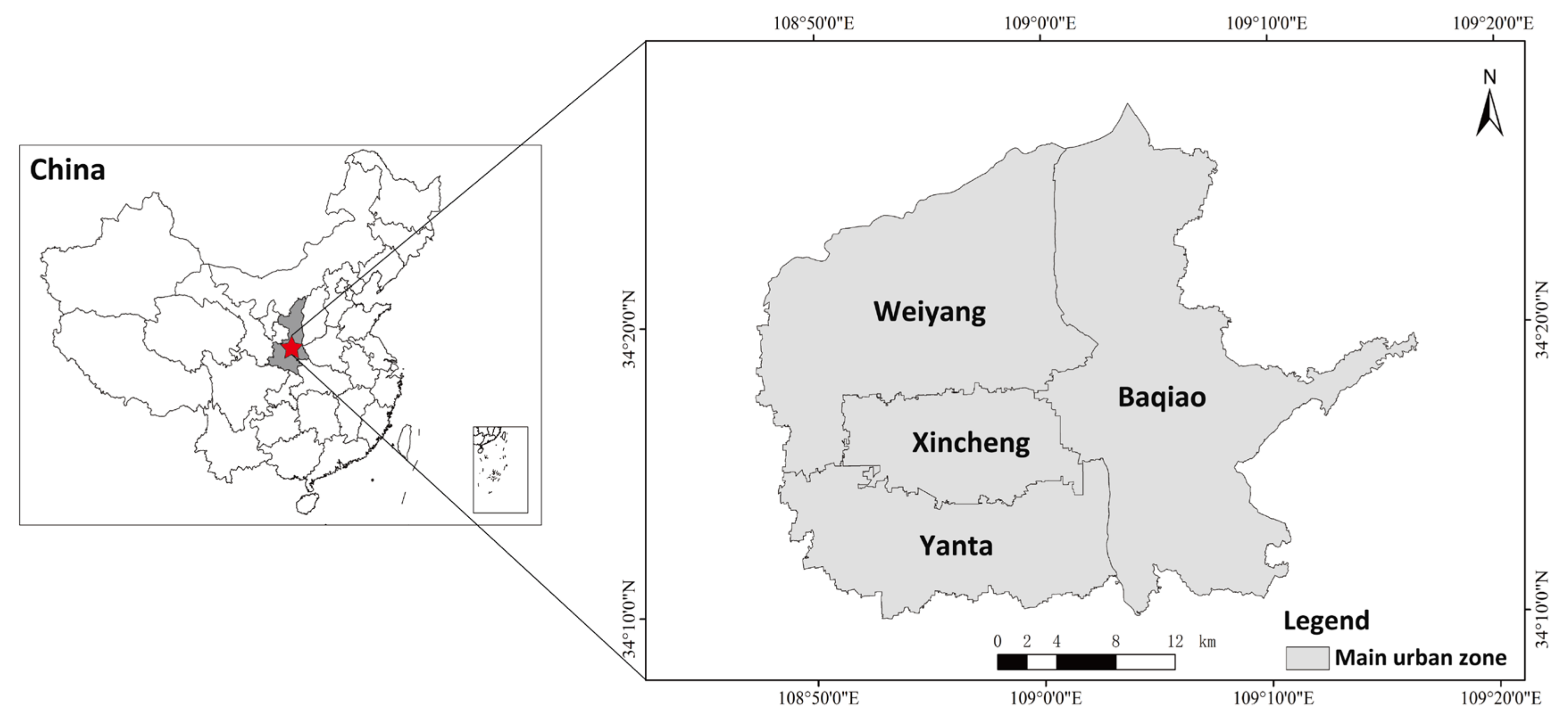
2.1. Study Area

Xi’an is located between 107°40′–109°49′ E and 33°39′–34°45′ N (Figure 1). The south and southeast sides are bounded by the main ridge of the Qinling Mountains, which serve as a natural boundary between the North and South part of China. The western, northwestern, and eastern sides of Xi’an are bounded by the Taibai Mountains, the Weihe River, and the Weihe Mountain, respectively. Xi’an is located in a river valley far from the sea, which makes the summer heat intense, and the cold air often stagnates on the ground in the winter. Xi’an has a continental climate with four distinct seasons—it is warm in spring, hot and humid in summer, cool in fall, and cold and dry in winter. In the urban green spaces, trees are mainly composed of Sophora japonica, Populus sp., Firmiana platanifolia, Cypress sp., and Pinus sp. The shrubs consist of Ligustrum quihoui, Buxus bodinieri, Berberis thunbergii var. atropurpurea, Buxus megistophylla, Photinia serrulata, and Pittosporum tobira, accounting for more than 80% of the total number of shrubs. The grasses include Poa annua, Festuca elata, Trifolium repens, Lolium perenne, and Ophiopogon japonicus. The population density of Xi’an city is 1185 per km2 and the impervious coverage percentage is 31.22% [34].

2.2. Data Source and Preprocessing

The data used in this study were obtained the Xi’an Urban Forest Resource Survey in 2006, while the field survey was conducted in 2017. In total, there were 1480 plots, covering four administrative districts (Baqiao, Weiyang, Xincheng, and Yanta) in the urban area (Figure 2). Each plot had 20 attributes surveyed in field work, including the forest class, land type, forestland ownership, forest ownership, forest category, authority, protection level, landform, slope, slope position, aspect, origin, dominant tree species, age group, accumulation per hectare, small class accumulation, and area. Of the 20 attributes, five were selected, including the dominant tree species, forest category, land types, age groups, and timber volume, due to these factors being the most relevant to the forest aboveground biomass. The first four attributes were used as potential factors affecting the biomass distribution, and the last one was used in the biomass calculation, which is explained in the following section.

2.3. Calculation of Aboveground Biomass for Urban Forests

The amount of forest stock comprehensively reflects the site conditions, climatic conditions, forest age, and other forest growth factors. Previous studies have found that the volume can be converted to biomass through a linear regression [35,36,37] (Equation (1)):
B = aV + b ,
where a and b are model parameter, depending on different tree types, and represent the slope and intercept in the linear regression function, respectively; B is the aboveground biomass, while V is the stock volume. Table 1 summarizes the a and b values for different tree species.

2.4. Spatial Analysis with the Geographical Detector

Geographical detectors (GDs) [38]—selected to study the forest biomass in our research—are widely used to examine geographical phenomena [21,38,39,40,41,42,43]. This approach can not only evaluate how certain geographical factors impact the spatial variable’s distribution, but also reveal the impacts of the interactions between the geographic factors on the spatial variables’ distribution.
The basic idea of a GD is to split the study area into subregions according to different categories of geographical factors (GFs). The variances of the dependent variable in each subregion and across the whole study area are compared to derive the impact of geographical factors on the dependent geographical variable’s spatial distribution. According to the principle of GD, the forest aboveground biomass, which is calculated by the stock volume, is used as the dependent variable. Moreover, four classes of multiple-level GFs (dominant tree species, forest categories, forestland class, and age groups at the plot level) are used as independent variables, and referred to as geographical factors. Each plot can be categorized into different numbers of subtypes according to different GFs (Table 2). In this study, the analysis focuses on four parts regarding the impacts of GFs on the spatial distribution of aboveground biomass: (a) Investigating whether there is spatial differentiation of biomass in the study area and how much each GF influences biomass; (b) examining the impacts of interactions between GFs; (c) comparing the impacts of different subcategories for each GF; and (d) comparing the impacts between different GFs.

2.4.1. Individual Impacts of GFs on the Spatial Distribution of Aboveground Biomass

To determine the extent of GFs’ impacts on the spatial differentiation of aboveground biomass in urban forests, Equation (2) [44] was adopted to calculate q for each GF:
q X = 1 h = 1 L X N h , X σ h , X 2 N σ total 2 ,
where h 1 , 2 , 3 , L X represents the category index for GF X. The forest   categories denote the type of geographical factor. L X is the number of total categories for GF X (in Table 2), N h ,   X is the number of plots in category h for geographical factor X, σ h , X 2 is the variance of biomass for plots in category h of geographical factor X, N is the total number of plots (i.e., 1480 in this study), and σ total 2 is the variance of biomass for all plots.
The range of q X is [0,1]. A larger q X value indicates that the variance of the aboveground biomass for plots within a subtype is more diverse between subtypes that are defined by categories of the GF X and vice versa. In extreme cases, a q X value of 1 indicates that the GF (X) completely controls the spatial distribution of aboveground biomass (Y), and a q X value of 0 indicates that the GF (X) has no relationship with the aboveground biomass (Y) of the urban trees.

2.4.2. Interaction Impacts of Geographical Factors on the Spatial Distribution of Aboveground Biomass

This study also investigates how the interaction between different GFs influences the spatial distribution of urban trees’ aboveground biomass. In other words, we want to reveal whether a given pair of GFs— X 1 and X 2 —interact to influence the explanatory power of the aboveground biomass (Y) distribution, or whether the influence of the GFs X 1 and X 2 on aboveground biomass (Y) of the forest are independent.
In this study, the interaction of a given combination of the GFs X 1 and X 2 , was written as X 1 X 2 . Additionally, q X 1 X 2 was calculated using Equation (2). The interaction could be classified as one of five groups by comparing q X 1 X 2 with the minimum, maximum, and sum of q X 1 and q X 2 [22].

2.4.3. Comparing the Impacts of Different Categories for Each GF

Given a GF X with two of its subtypes h 1 and h 2 , we applied Tukey’s Honestly Significant Differences (Tukey’s HSD) test to examine whether the average plot’s aboveground biomass in subtypes h 1 was significantly different from it in h 2   using Equations (3) and (4):
H S D 0.05 h 1 , h 2 = q 0.05 2 , n 2 1 2 M S e 1 r 1 + 1 r 2 ,
H S D h 1 , h 2 = Y ¯ h 1 Y ¯ h 2 ,
where n is the total number of plots (i.e., 1480 in this study); q 0.05 2 , n 2   is the quantile of the Studentized range distribution M S e stands for the mean sum of squares of deviation within groups in ANOVA; r 1 and r 2 represent the number of plots of subtypes h 1 and h 2 , respectively ; Y ¯ h 1 and Y ¯ h 2 represent the average aboveground biomass of subtypes h 1 and h 2 , respectively. The null hypothesis H0 for the test is Y ¯ h 1 = Y ¯ h 2 . A rejection of H0 means that there is a significant difference between the average plot aboveground biomass within subregions h 1 and h 2 . If H S D h 1 , h 2 H S D 0.05 h 1 , h 2 , H0 can be accepted, and it is believed that there is no significant difference between the average plot’s aboveground biomass within subregions h 1 and h 2 .

2.5. Comparing the Impacts for Different GFs

To investigate whether a combination of the two GFs X1 and X2 exhibits significant differences in terms of the spatial distribution of aboveground biomass (Y) in urban forests, a F-statistic was calculated using Equations (5)–(7):
F = N X 1 N X 2 1 SSW X 1 N X 2 N X 1 1 SSW X 2 ,
SSW X 1 = h = 1 L 1 N h σ h 2 ,
SSW X 2 = h = 1 L 2 N h σ h 2 ,
where N X 1 and N X 2 represent the sample sizes of X1 and X2, respectively;   SSW X 1 and SSW X 2 represent the sum of the intralayer variances of the layers formed by X1 and X2, respectively; and L1 and L2 represent the number of layers defined by X1 and X2, respectively. The null hypothesis of the F-test is H 0 : SSW X 1 = SSW X 2 . If H 0 is rejected at the level of significance of α, it indicates that X1 and X2 display significant differences in relation to the spatial distribution of aboveground biomass (Y) in urban forests.

3. Results

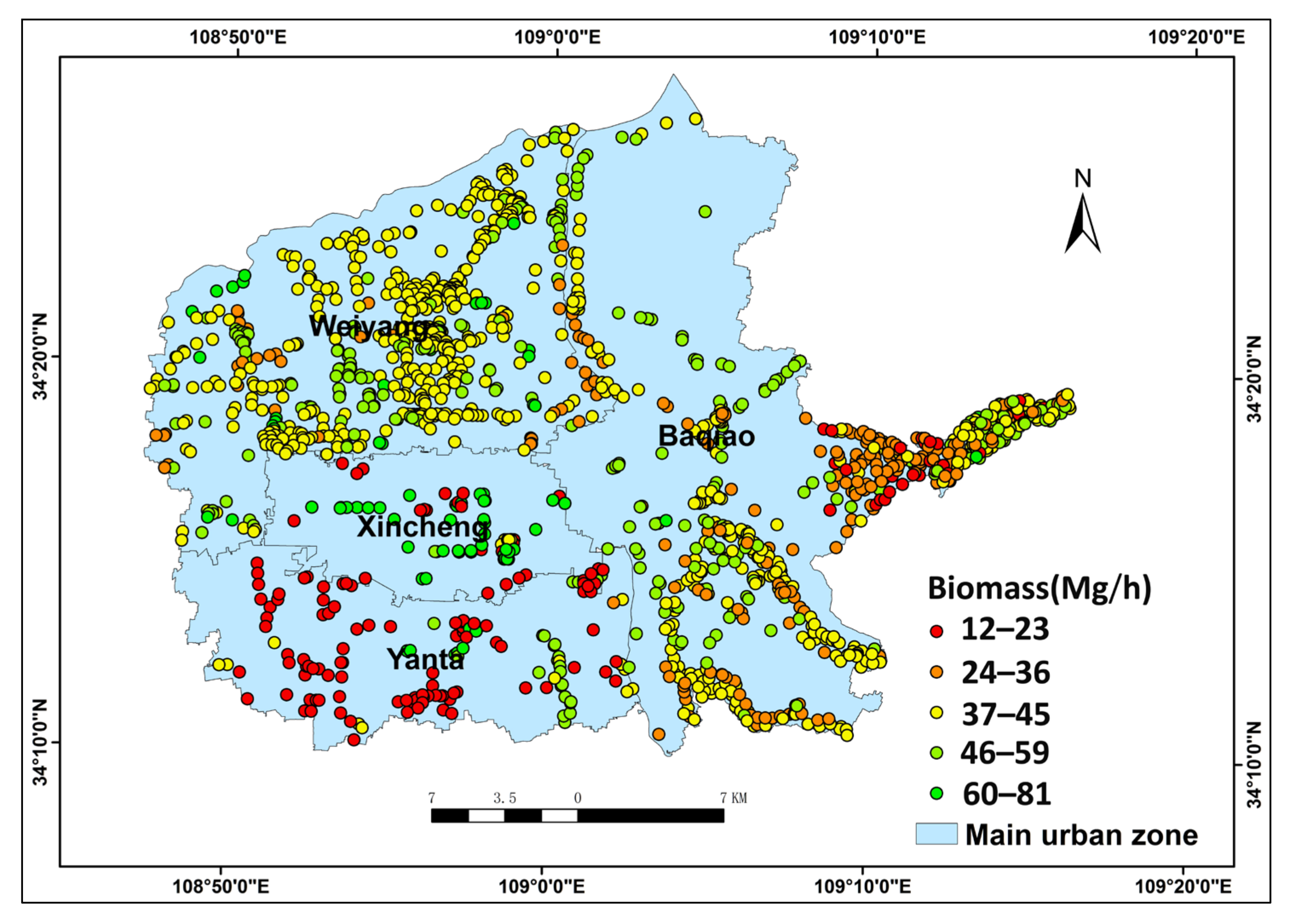
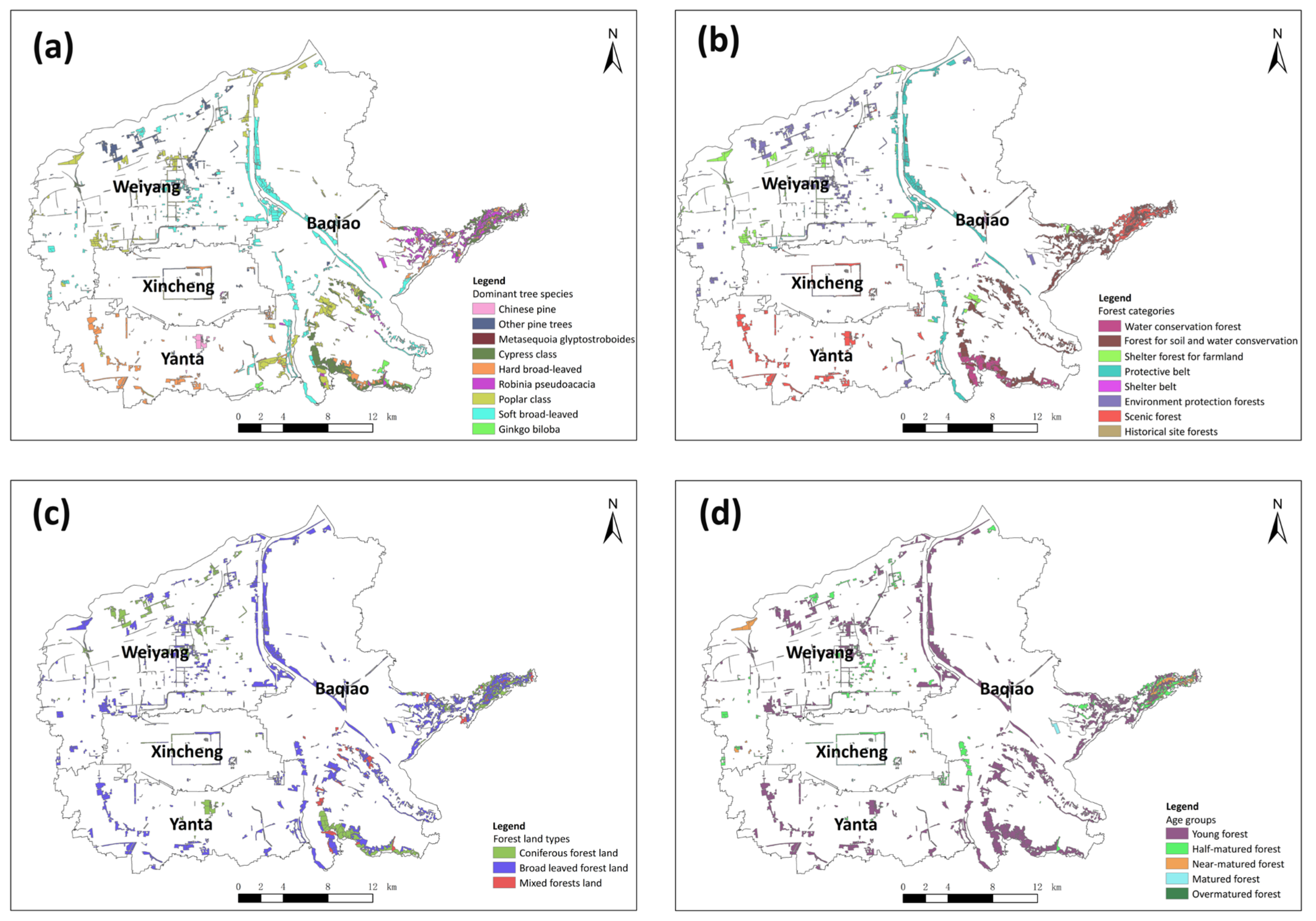
3.1. The Distributions of Urban Forest Biomass and Its Influencing Factors

The biomass of 1480 plots shows significant spatial differences (Figure 2). The biomass distribution of plots reflects that the urban forests are mainly distributed in the northwestern, southeastern and the eastern part of Xi’an. The biomass in the northwestern part (Weiyang), with 611 plots and 44.77% of the total forest biomass, primarily consists of the urban garden and protected area. The biomass in the southeast and east exhibits a highly positive relationship with rivers. The highest biomass can be observed in the central area of Xi’an (Xincheng) city, with 83 plots and 6.89% of the total forest biomass, and with the average biomass reaching to 59.25 Mg/h. The biomass in the southern part of Xi’an (Yanta), with 143 plots and 6.64% of the total forest biomass, is the lowest (lower than 22.63 Mg/h). This is because Yanta is a newly developing urban area, and the trees there are almost young forest trees. The northwestern part of Xi’an has medium level of biomass. The eastern part of Xi’an (Baqiao), with 643 plots and 41.7% of the total forest biomass, exhibits a relatively lower biomass than southern Xi’an.
Four influencing factors, including the dominant tree species, forest categories, forestland types, and age groups, present spatial heterogeneity (Figure 3). The dominant tree species which are distributed with a patch pattern are mostly located along the road and in the urban garden (Figure 3a). Pinus and hardwood forests are mainly distributed in Yanta District. Populus is distributed in Weiyang and Baqiao District. Platycladus orientalis is distributed in the south of Baqiao District for the most part. Most of the hardwood trees are found in the west of Yanta District. Robinia pseudoacacia is commonly found in eastern Baqiao District. The softwood trees display a significant positive relationship with rivers. Ginkgo biloba is mainly distributed in the middle of the south of Yanta District, in a small area.
Figure 3b shows the distribution of forest categories. Forests for water conservation are mainly distributed in the south of Baqiao District. Forests for soil conservation are mainly found in the south and east of Baqiao District. Forests for protecting farms are mainly located in the south of Weiyang and Baqiao Districts, with a small area. Forests for shore protection are distributed on both sides of most rivers. Forests for protecting the environment are situated in Weiyang District, while the landscape forests are mainly distributed in Yanta District. Other types of forests exhibit a sporadic distribution, with a small area.
Figure 3c shows the distribution of land types. The needleleaf forestland is mainly distributed in the south of Weiyang and Baqiao Districts. The broadleaf forestland has the largest area and is found everywhere in the study area. The mingled forestland is mainly located in the south and east of Baqiao District. Figure 3d shows the age distribution. Most forests are young in age, while mature and overmatured forests are scarce in the four districts of Xi’an.

3.2. Detecting the Contribution of the Four Influencing Factors

The independent q values of the four influencing factors ranged from 8% to 59% (Table 3). The results of Equation (2) showed that the contribution of each impact factor towards the differentiation of the spatial distribution of aboveground biomass is ordered as follows: Dominant tree species, age group, forest category, and land type. The first two factors (with q value > 0.20) are considered to be the major impact factors.
Ecological detectors can reflect significant differences among the four GFs regarding their impacts on the biomass of forests. As shown in Table 4 (generated by the F-test with Equation (5)), the forest age is significantly different from the other factors. The forestland types only differ from the dominant species, and show no difference from the forest types. The forest type displays a significant difference when compared to the dominant tree species, but shows no significant difference with the forest tree species. The forest tree species is significantly different from the dominant tree species.

3.3. Detecting the Contribution of Interactions between the Four Influencing Factors

In the forest environment, the forest aboveground biomass is the result of a combination of multiple factors, and is also influenced by interactions between these factors. The spatial distribution of aboveground biomass in urban forests is always affected by various factors, as well as their interactions with each other, but not by single factors. According to Table 5, our results (Table 6) show that the interaction between GFs mainly involves nonlinear enhancement, indicating that the interaction between GFs’ impact is larger than the simple combination of individual factors.
To quantify the synergistic effects, we combined the ratios of interactions and the combined effect was calculated. A larger ratio value means that stronger synergistic effects exist between GFs. Among all the pairs of GFs, the synergistic effects between the forest category and land types are greater than the rest of the pairs, and show the highest ratio value (1.65). Furthermore, the ratio of the dominant tree species and land type exhibits the weakest synergistic effects.

3.4. Comparing the Difference of the Contribution among Subtypes

The pairwise comparison results, using Tukey’s Honestly Significant Differences test for the forestland type (Table 7), show that the average plot’s biomass in coniferous forestland was significantly higher than that in broad-leaved forestland and mixed forestland. Furthermore, there was no significant difference between mixed forestland and broad-leaved forestland regarding the average plot’s biomass.
The Tukey’s HSD test, comparing the average plot’s biomass for different tree species shows that the plot dominated by Ginkgo biloba had a significantly higher average plot’s biomass than other species, expect for the Poplar class and Parker class (Appendix A Table A1). These species are the major greening tree species in green spaces in Xi’an city [45]. They exhibit a considerable tolerance for gaseous air pollutants, but are susceptible to damage from acid rain [46,47,48]. Due to the “Coal to Gas Project” implemented in 1997 [49], the emergence rate of acid rain has obviously decreased [50], providing favorable growth conditions for these species, rather than Pinus tabuliformis and Robinia pseudoacacia.
A comparison of the average plot’s biomass among the eight subtypes defined by forest functionalities showed that the difference between these types is generally not as significant as those between subtypes defined by dominant tree species (Appendix A Table A2). Among the eight subtypes, even though historical site forests retain the largest average plot’s biomass, they only displayed significant differences from forest for soil and water conservation and scenic forests. With the lowest mean value of the plot’s biomass, scenic forest displayed a significant difference from all other forests, except for the water conservation forest and forest for soil and water conservation.
The investigation of the age group factors shows that all subtypes split by forest age group are significantly different from each other, regarding the average plot’s biomass in the subtypes (Appendix A Table A3). If GD is used as a tool to detect the overall picture of impacts for all the GFs, then Tukey’s HSD test can be thought of as a magnifier, showing details of how the elements within each GF exerting impacts.

4. Discussion

4.1. The Significance of Studying the Spatial Heterogeneity of Urban Forest Biomass

In this study, we analyzed the spatial heterogeneity of urban forest’s aboveground biomass and can conclude that the dominant tree species and age group are the main factors impacting the biomass distribution. These results are consistent with previous studies [51,52]. Detecting the drivers of urban forest biomass is important for the urban forest management. Among the four main drivers, we found that the tree species is the most critical factor affecting the urban forests’ aboveground biomass. This result agrees with Shuaifeng Li. et al. [53], who reported that the species richness had a positive impact on aboveground biomass across all forest vegetation layers. This result means that the choice of planted tree species could determine the pattern of urban forest. Therefore, trees with fast growth rates should be considered first. This study also indicates that the interaction effect of two factors is greater than that of a single one, which is also reflected in the nonlinear relation model in urban forest modeling [54]. The results of interactions mean that we should not only focus on the independent role of single driving factors, but also pay more attention to their interaction, which may greatly improve the productivity of urban forests.
Investigating how different GFs drive the distribution of urban forests’ aboveground biomass could provide important implications for better urban planning, which responds to urban atmosphere changes and the development of sustainable urbanization. As an important carrier of the urban ecosystem, urban forests offer ecological, economic, and social benefits for human beings. They can not only improve the urban microclimate, alleviate the effects of urban heat islands, increase surface runoff, and play an important role in maintaining the urban carbon and oxygen balance, but also improve the quality of life of residents and provide good places of leisure and entertainment for urban residents [55,56]. Urban forest biomass is an important indicator that can be used to measure the carbon storage, carbon sequestration capacity, and ecological benefits of an urban ecosystem [57]. The accurate and rapid monitoring of urban forest biomass and its spatial pattern are the basis for urban carbon cycle and energy flow research, while they are also the basis for measuring the ecological regulation and environmental protection capacity of urban forests [58]. Analyzing the spatial differentiation of urban forest biomass can provide data for the urban green space planning department, and has great significance for urban ecological space planning and management.

4.2. Challenges and Future Directions

Forest biomass is affected by several variables, including human activities, as well as environmental and biological factors [59]. It shows a certain randomness and distribution with structural differences. The spatial heterogeneity of forest biomass reflects the energy flows and material cycles of forest ecosystems [60,61]. The study area is a plain, and its internal environmental factors (such as its topography and climate) can be considered to be uniform. Based on these conditions, forest resource survey data of the study area were employed, while four qualitative factors (land type, forest category, age group, and dominant tree species) were selected to study the spatial heterogeneity and the influencing factors of urban forest biomass by using the geographic detector method. This approach obtains a quantitative description of qualitative influencing factors and solves the problem of collinearity that has often been ignored in past related research. However, the following aspects should be considered in future related research: (1) In addition to the four factors mentioned above, there are many factors, (i.e., average tree species, average DBH, and human activities) that required further comprehensive analysis in the future; (2) in this study, the spatial heterogeneity of aboveground forest biomass is mainly discussed. However, the biomass of shrubs, herbs, and underground parts of the forest was not considered; and (3) in this study, calculation of the biomass of forestland was obtained from forest resource investigation data. In future related research, using remote sensing technology to retrieve biomass directly is recommended. Therefore, we could quickly analyze the spatial heterogeneity of forest biomass [62].

5. Conclusions

In this study, we conducted spatial statistical analysis by the GD method to systematically study the differentiation of the urban forest biomass distribution of Xi’an. Additionally, we examined how dominant tree species, age groups, forest categories, and forestland types individually and interactively impacted the urban forest biomass distribution. We concluded that: (1) among the four GFs, including dominant tree species, forest species, land types, and age groups, the spatial distribution of aboveground forest biomass in Xi’an is primarily influenced by dominant tree species and forest age. Their combined effects account for 80% of the total impacts; (2) there is no significant difference between forestland and forest categories regarding their impacts on the spatial distribution of aboveground biomass; and (3) all of the pairs of the four GFs have nonlinear enhancement effects, except for the bilinear enhancement effect between dominant tree species and the land type. Among all pairs of GFs, the synergistic effect is most obvious for the interaction between the forest category and land type. Overall, the results of urban forest biomass’ spatial heterogeneity among these GFs can help researchers’ understanding of urban forest biomass change, which may be applied in future precise forest prediction models on a larger scale and allow for more effective forest management strategies to be developed.

Author Contributions

Conceptualization, Xuan Zhao; data curation, Xuan Zhao; formal analysis, Xuan Zhao; funding acquisition, Jianjun Liu; investigation, Hongke Hao; methodology, Xuan Zhao; project administration, Jianjun Liu; resources, Yanzheng Yang. All authors have read and agreed to the published version of the manuscript.

Funding

This research was primarily funded by Research on Vegetation Restoration Techniques on Steep Loess Slope in Qianyang, Shanxi, grant number K303021613.

Acknowledgments

We thank the funding of “Research on Vegetation Restoration Techniques on Steep Slope of Loess in Qianyang, Shaanxi”.

Conflicts of Interest

The authors declare no conflict of interest.

Appendix A

Table A1. Tukey’s Honestly Significant Differences (Tukey’s HSD) test for the dominant tree species factor (Y means the testing is significant at the 0.05 level, and N represents an insignificant difference).
Chinese PineOther Pine TreesMetasequoia GlyptostroboidesParker ClassHard Broad-LeavedRobinia PseudoacaciaPoplar ClassSoft Broad-LeavedGinkgo Biloba
Chinese pine-Y-YNYYYY18.4
Other pine treesY--YYYYYN49.9
Metasequoia glyptostroboides---------58.6
Parker classYY--YYYYY44.0
Hard broad-leavedNY-Y-YYYY19.6
Robinia pseudoacaciaYY-YY-YYY32.9
Poplar classYY-YYY-YN47.3
Soft broad-leavedYY-YYYY-Y38.6
Ginkgo bilobaYN-YYYNY-56.3
18.449.958.644.019.632.947.338.656.3
Table A2. Tukey’s HSD test for the forest category factor (Y means the testing is significant at the 0.05 level, and N represents an insignificant difference).
Water Conservation ForestForest for Soil and Water ConservationShelter Forest for FarmlandProtective BeltShelter BeltEnvironmental Protection ForestsScenic ForestHistorical Sites Forests
Water conservation forest-NNNNNNN38.6
Forest for soil and water conservationN-YYNYNY36.3
Shelter forest for farmlandNY-NNNYN43.9
Protective beltNYN-NNYN41.5
Shelter beltNNNN-NNN41.5
Environmental protection forestsNYNNN-YN43.3
Scenic forestNNYYNY-Y35.7
Historical sites ForestsNYNNNNY-64.4
38.636.343.941.541.543.335.764.4
Table A3. Tukey’s HSD test for age group factor (Y means the testing is significant at the 0.05 level, and N represents an insignificant difference).
Young ForestHalf-Mature ForestNear-Mature ForestMature ForestOvermature Forest
Young forest-YYY-37.5
Half-mature forestY-YY-43.1
Near-mature forestYY-Y-54.2
Mature forestYYY--78.6
Overmature forest-----55.7
37.543.154.278.655.7

References

  1. United Nations. World Urbanization Prospects: The 2018 Revision; United Nations Publications: New York, NY, USA, 2019. [Google Scholar]
  2. Collier, P.; Venables, A.J. Urbanization in developing economies: The assessment. Oxf. Rev. Econ. Policy 2017, 33, 355–372. [Google Scholar] [CrossRef]
  3. World Urbanization Prospects. Available online: https://esa.un.org/unpd/wup/publications/fles/wup2014-highlights.Pdf (accessed on 11 November 2014).
  4. China Statistical Yearbook. Available online: http://www.stats.gov.cn/tjsj/ndsj/2018/indexch.htm (accessed on 29 November 2018).
  5. Zhang, Z.B. Report on the Healthy Development of China’s New Urbanization (2016); Social Science Literature Press: Beijing, China, 2017. [Google Scholar]
  6. Orum, A.M.; Iossifova, D. East Asian Urbanization. In The Wiley Blackwell Encyclopedia of Urban and Regional Studies; Orum, A.M., Ed.; John Wiley & Sons: Hoboken, NJ, USA, 2019. [Google Scholar] [CrossRef]
  7. Bolund, P.; Hunhammar, S. Ecosystem services in urban areas. Ecol. Econ. 1999, 29, 293–301. [Google Scholar] [CrossRef]
  8. Nowak, D.J.; Greenfield, E.J.; Hoehn, R.E.; Lapoint, E. Carbon storage and sequestration by trees in urban and community areas of the United States. Environ. Pollut. 2013, 178, 229–236. [Google Scholar] [CrossRef] [PubMed] [Green Version]
  9. Timilsina, N.; Staudhammer, C.L.; Escobedo, F.J.; Lawrence, A. Tree biomass, wood waste yield, and carbon storage changes in an urban forest. Landsc. Urban Plan. 2014, 127, 18–27. [Google Scholar] [CrossRef]
  10. Abdi, R.; Endreny, T.; Nowak, D. A model to integrate urban river thermal cooling in river restoration. J. Environ. Manag. 2020, 258, 110023. [Google Scholar] [CrossRef] [PubMed]
  11. Elmqvist, T.; Fragkias, M.; Goodness, J.; Güneralp, B.; Marcotullio, P.J.; McDonald, R.I.; Parnell, S.; Schewenius, M.; Sendstad, M.; Seto, K.C.; et al. Urbanization, Biodiversity and Ecosystem Services: Challenges and Opportunities: A Global Assessment; Springer: Dordrecht, The Netherlands, 2013. [Google Scholar] [CrossRef] [Green Version]
  12. Nowak, D.J.; Daniel, E.C. Carbon storage and sequestration by urban trees in the USA. Environ. Pollut. 2002, 116, 381–389. [Google Scholar] [CrossRef]
  13. Nowak, D.J. Atmospheric carbon dioxide reduction by Chicago’s urban forest. In Chicago’s Urban Forest Ecosystem: Results of the Chicago Urban Forest Climate Project; Forest Service US: Washington, DC, USA, 1994; pp. 83–94. Available online: https://www.fs.usda.gov/treesearch/pubs/4285 (accessed on 11 December 2020).
  14. Li, L.; Zhou, X.; Chen, L.; Chen, L.; Zhang, Y.; Liu, Y. Estimating urban vegetation biomass from Sentinel-2A image data. Forests 2020, 11, 125. [Google Scholar] [CrossRef] [Green Version]
  15. Hu, S.; Chen, L.; Li, L.; Zhang, T.; Yuan, L.; Cheng, L.; Wang, J.; Wen, M. Simulation of Land Use Change and Ecosystem Service Value Dynamics under Ecological Constraints in Anhui Province, China. Int. J. Environ. Res. Public Health 2020, 17, 4228. [Google Scholar] [CrossRef]
  16. McPherson, E.G. Atmospheric carbon dioxide reduction by Sacramento’s urban forest. J. Arboric. 1998, 24, 215–223. [Google Scholar]
  17. Aguaron, E.; McPherson, E.G. Comparison of methods for estimating carbon dioxide storage by Sacramento’s urban forest. In Carbon Sequestration in Urban Ecosystems; Springer: Dordrecht, The Netherlands, 2012; pp. 43–71. [Google Scholar] [CrossRef]
  18. Rowntree, R.A.; Nowak, D.J. Quantifying the role of urban forests in removing atmospheric carbon dioxide. J. Arboric. 1991, 17, 269–275. [Google Scholar]
  19. Dutilleul, P.R.L. Spatio-Temporal Heterogeneity: Concepts and Analyses; Cambridge University Press: Cambridge, UK, 2011. [Google Scholar]
  20. Wang, J.F.; Zhang, T.L.; Fu, B.J. A measure of spatial stratified heterogeneity. Ecol. Indic. 2016, 67, 250–256. [Google Scholar] [CrossRef]
  21. Wang, J.F.; Li, X.H.; Christakos, G.; Liao, Y.L.; Zhang, T.; Gu, X.; Zheng, X.Y. Geographical detectors-based health risk assessment and its application in the neural tube defects study of the Heshun region, China. Int. J. Geogr. Inf. Sci. 2010, 24, 107–127. [Google Scholar] [CrossRef]
  22. Wang, J.F.; Xu, C.D. Geodetector: Principle and prospective. Acta Geogr. Sin. 2017, 72, 116–134. [Google Scholar]
  23. Li, M.; Im, J.; Quackenbush, L.J.; Liu, T. Forest biomass and carbon stock quantification using airborne LiDAR data: A case study over Huntington Wildlife Forest in the Adirondack Park. IEEE J. Sel. Top. Appl. Earth Obs. Remote Sens. 2014, 7, 3143–3156. [Google Scholar] [CrossRef]
  24. Gleason, C.J.; Im, J. Forest biomass estimation from airborne LiDAR data using machine learning approaches. Remote Sens. Environ. 2012, 125, 80–91. [Google Scholar] [CrossRef]
  25. Rauf, A. Distribution, above-ground biomass and carbon stock of the vegetation in Taman Beringin Urban Forest, Medan City, North Sumatra, Indonesia. Malays. For. 2017, 80, 73–84. [Google Scholar]
  26. Pesola, L.; Cheng, X.; Sanesi, G.; Colangelo, G.; Elia, M.; Lafortezza, R. Linking above-ground biomass and biodiversity to stand development in urban forest areas: A case study in Northern Italy. Landsc. Urban Plan. 2017, 157, 90–97. [Google Scholar] [CrossRef]
  27. Shen, G.; Wang, Z.; Liu, C.; Han, Y. Mapping aboveground biomass and carbon in Shanghai’s urban forest using Landsat ETM+ and inventory data. Urban For. Urban Greening 2020, 51, 126655. [Google Scholar] [CrossRef]
  28. Baker, T.R.; Phillips, O.L.; Malhi, Y.; Almeida, S.; Arroyo, L.; di Fiore, A.; Erwin, T.; Killeen, T.J.; Laurance, S.G.; Laurance, W.F.; et al. Variation in wood density determines spatial patterns in Amazonian forest biomass. Glob. Chang. Biol. 2004, 10, 545–562. [Google Scholar] [CrossRef]
  29. López-Serrano, P.M.; Corral-Rivas, J.J.; Díaz-Varela, R.A.; Álvarez-González, J.G.; López-Sánchez, C.A. Evaluation of radiometric and atmospheric correction algorithms for aboveground forest biomass estimation using Landsat 5 TM data. Remote Sens. 2016, 8, 369. [Google Scholar] [CrossRef] [Green Version]
  30. Luo, S.; Wang, C.; Xi, X.; Nie, S.; Fan, X.; Chen, H.; Ma, D.; Liu, J.; Zou, J.; Lin, Y.; et al. Estimating forest aboveground biomass using small-footprint full-waveform airborne LiDAR data. Int. J. Appl. Earth Obs. Geoinf. 2019, 83, 101922. [Google Scholar] [CrossRef]
  31. Fassnacht, F.E.; Hartig, F.; Latifi, H.; Berger, C.; Hernández, J.; Corvalán, P.; Koch, B. Importance of sample size, data type and prediction method for remote sensing-based estimations of aboveground forest biomass. Remote Sens. Environ. 2014, 154, 102–114. [Google Scholar] [CrossRef]
  32. Foody, G.M.; Cutler, M.E.; McMorrow, J.; Pelz, D.; Tangki, H.; Boyd, D.S.; Douglas, I.A.N. Mapping the biomass of Bornean tropical rain forest from remotely sensed data. Glob. Ecol. Biogeogr. 2001, 10, 379–387. [Google Scholar] [CrossRef]
  33. Kimes, D.S.; Nelson, R.F.; Manry, M.T.; Fung, A.K. Attributes of neural networks for extracting continuous vegetation variables from optical and radar measurements. Int. J. Remote Sens. 1998, 19, 2639–2663. [Google Scholar] [CrossRef]
  34. Xi’an 2015 National Economic and Social Development Statistical Bulletin. Available online: www.xatj.gov.cn (accessed on 12 December 2016).
  35. Fang, J.; Liu, G.; Xu, S. Biomass and net production of forest vegetation in China. Acta Ecol. Sin. 1996, 16, 497–508. (In Chinese) [Google Scholar]
  36. Fang, J.Y.; Wang, G.G.; Liu, G.H.; Xu, S.L. Forest biomass of China: An estimate based on the biomass—Volume relationship. Ecol. Appl. 1998, 8, 1084–1091. [Google Scholar]
  37. Fang, J.; Chen, A.; Peng, C.; Zhao, S.; Ci, L. Changes in forest biomass carbon storage in China between 1949 and 1998. Science 2001, 292, 2320–2322. [Google Scholar] [CrossRef]
  38. Luo, W.; Jasiewicz, J.; Stepinski, T.; Wang, J.; Xu, C.; Cang, X. Spatial association between dissection density and environmental factors over the entire conterminous United States. Geophys. Res. Lett. 2016, 43, 692–700. [Google Scholar] [CrossRef] [Green Version]
  39. Liao, Y.; Wang, J.; Wu, J.; Driskell, L.; Wang, W.; Zhang, T.; Xue, G.; Zheng, X. Spatial analysis of neural tube defects in a rural coal mining area. Int. J. Environ. Health Res. 2010, 20, 439–450. [Google Scholar] [CrossRef]
  40. Hu, Y.; Wang, J.; Li, X.; Ren, D.; Zhu, J. Geographical detector-based risk assessment of the under-five mortality in the 2008 Wenchuan earthquake, China. PLoS ONE 2011, 6, e21427. [Google Scholar] [CrossRef] [Green Version]
  41. Zou, B.; Wilson, J.G.; Zhan, F.B.; Zeng, Y.; Wu, K. Spatial-temporal variations in regional ambient sulfur dioxide concentration and source-contribution analysis: A dispersion modeling approach. Atmos. Environ. 2011, 45, 4977–4985. [Google Scholar] [CrossRef]
  42. Wang, J.F.; Hu, Y. Environmental health risk detection with GeogDetector. Environ. Model. Softw. 2012, 33, 114–115. [Google Scholar] [CrossRef]
  43. Zhu, Z.; Wang, J.; Hu, M.; Jia, L. Geographical detection of groundwater pollution vulnerability and hazard in karst areas of Guangxi Province, China. Environ. Pollut. 2019, 245, 627–633. [Google Scholar] [CrossRef] [PubMed]
  44. Wang, F.; Liao, L.; Liu, X. Spatial Analysis Tutorial; Science Press: Beijing, China, 2010. [Google Scholar]
  45. Yao, Z.; Liu, J.; Zhao, X.; Long, D.; Wang, L. Spatial dynamics of aboveground carbon stock in urban green space: A case study of Xi’an, China. J. Arid. Land 2015, 7, 350–360. [Google Scholar] [CrossRef]
  46. Kim, Y.S.; Lee, J.K.; Chung, G.C. Tolerance and susceptibility of Ginkgo to air pollution. In Ginkgo Biloba A Global Treasure; Springer: Tokyo, Japan, 1997; pp. 233–242. [Google Scholar] [CrossRef]
  47. Matyssek, R.; Giinthardt-Goerg, M.S.; Schmutz, P.; Saurer, M.; Landolt, W.; Bücher, J.B. Response mechanisms of birch and poplar to air pollutants. J. Sustain. For. 1997, 6, 3–22. [Google Scholar] [CrossRef]
  48. Barwise, Y.; Prashant, K. Designing vegetation barriers for urban air pollution abatement: A practical review for appropriate plant species selection. npj Clim. Atmos. Sci. 2020, 3, 1–19. [Google Scholar] [CrossRef] [Green Version]
  49. Miao, J.L. Analysis of climatic characteristics and meteorological conditions of acid rain in Xi’an. Shaanxi Meteorol. 2013, 36–39. (In Chinese) [Google Scholar] [CrossRef]
  50. Xi’an Environmental Status Bulletin. 2017. Available online: http://xaepb.xa.gov.cn/xxgk/hjzkgb/hjzkgb/5d8b5a9cf99d65052290af21.html (accessed on 18 December 2018).
  51. Cheng, Y.; Zhang, C.; Zhao, X.; von Gadow, K. Biomass-dominant species shape the productivity-diversity relationship in two temperate forests. Ann. For. Sci. 2018, 75, 1–9. [Google Scholar] [CrossRef] [Green Version]
  52. Chen, Z.; Yu, G.; Wang, Q. Effects of climate and forest age on the ecosystem carbon exchange of afforestation. J. For. Res. 2020, 31, 365–374. [Google Scholar] [CrossRef] [Green Version]
  53. Li, S.; Su, J.; Lang, X.; Liu, W.; Ou, G. Positive relationship between species richness and aboveground biomass across forest strata in a primary Pinus kesiya forest. Sci. Rep. 2018, 8, 1–9. [Google Scholar] [CrossRef]
  54. Zhao, K.; Popescu, S.; Nelson, R. Lidar remote sensing of forest biomass: A scale-invariant estimation approach using airborne lasers. Remote Sens. Environ. 2009, 113, 182–196. [Google Scholar] [CrossRef]
  55. Singh, K.K.; Gagné, S.A.; Meentemeyer, R.K. Urban Forests and Human Well-Being. Compr. Remote Sens. 2018, 287–305. [Google Scholar] [CrossRef]
  56. Christine, B.; Katrin, R. The role of urban green space for human well-being. Ecol. Econ. 2015, 120, 139–152. [Google Scholar]
  57. Kang, M.N.; Shawn, L. Aboveground biomass estimation of tropical street trees. J. Urban Ecol. 2018, 4, 1–6. [Google Scholar]
  58. Wang, Z.; Shen, G.; Zhu, Y.; Liu, C. Spatiotemporai dynamics of urban forest biomass in Shanghai, China. In Proceedings of the 2015 Fourth International Conference on Agro-geoinformatics, Istanbul, Turkey, 20–24 July 2015. [Google Scholar]
  59. Zhang, H.; Song, T.; Wang, K.; Yang, H.; Yue, Y.; Zeng, Z.; Peng, W.; Zeng, F. Influences of stand characteristics and environmental factors on forest biomass and root–shoot allocation in southwest China. Ecol. Eng. 2016, 91, 7–15. [Google Scholar] [CrossRef]
  60. Edna, R.; Matthias, C.; Jens, H.; Anja, R.; Andreas, H. Spatial heterogeneity of biomass and forest structure of the Amazon rain forest: Linking remote sensing, forest modelling and field inventory. Glob. Ecol. Biogeogr. 2017, 26, 1–11. [Google Scholar]
  61. Röser, D.; Asikainen, A.; Raulund-Rasmussen, K.; Stupak, I. Sustainable Use of Forest Biomass for Energy; Managing Forest Ecosystems: New York, NY, USA, 2008. [Google Scholar] [CrossRef]
  62. Zhang, X.; Ni-meister, W. Remote Sensing of Forest Biomass. Biophys. Appl. Satell. Remote Sens. 2013, 63–98. [Google Scholar] [CrossRef]
Figure 1. Location of the study area.
Ijgi 09 00744 g001
Figure 2. Distribution of biomass grades of 1480 plots.
Ijgi 09 00744 g002
Figure 3. The whole study area was split into different subtypes according to GFs: (a) Dominant tree species; (b) forest categories; (c) forestland types; and (d) age groups.
Ijgi 09 00744 g003
Table 1. Conversion model parameters between the aboveground biomass and stock volume for different tree species [35].
Serial NumberTree SpeciesabR2Tree Type
1Chinese pine0.75545.09280.980Coniferous tree
2Other pine trees0.516833.23780.970Coniferous tree
3Metasequoia glyptostroboides0.415841.33180.980Coniferous tree
4Cypress class0.612926.14510.980Coniferous tree
5Hard broad-leaved0.96440.84850.980Deciduous tree
6Robinia pseudoacacia0.75648.31030.986Deciduous tree
7Poplar class0.475430.60340.930Deciduous tree
8Soft broad-leaved0.475430.60340.930Deciduous tree
9Ginkgo biloba0.415841.33180.980Deciduous tree
Table 2. Four geographical factors (GFs) and their categories.
GFsCategoriesNumber of Categories
Dominant tree speciesChinese pine, Other pine trees, Metasequoia glyptostroboides, Parker class, Hard broad-leaved, Robinia pseudoacacia, Poplar class, Soft broad-leaved, and Ginkgo biloba9
Forest categoriesWater conservation forests, Forest for soil and water conservation, Shelter forest for farmland, Protective belt, Shelter belts, Environmental protection forests, Scenic forests, and Historical site forests8
Forestland typesConiferous forestland, Broad leaved forestland, Mixed forestland3
Age groupsYoung forest, Half-matured forest, Near-matured forest, Matured forest, Overmatured forest5
Table 3. The independent q values of the four GFs.
Dominant Tree SpeciesAge GroupForest CategoryLand Type
0.5950.2020.0870.076
Table 4. Significant differences in reflecting forest aboveground biomass among influencing factors.
Dominant Tree SpeciesForest CategoryForestland TypeAge Group
Dominant tree species-YYY
Forest categoryY-NY
Forestland typeYN-Y
Age groupYYY-
Note: Y means the null hypothesis is rejected at a significance level of 0.05, while N means no significant difference between the average plot’s biomass.
Table 5. Interaction derivation [9].
Comparison TypeInteraction
q X 1 X 2   <   min ( q X 1 ,   q X 2 ) Weaken, nonlinear
min ( q X 1 ,   q X 2 )   <   q X 1 X 2   <   max ( q X 1 ,   q X 2 ) Weaken, single factor nonlinear
q X 1 X 2   >   max ( q X 1 ,   q X 2 ) Enhance, bilinear
q X 1 X 2 = q X 1 + q X 2 Independent
q X 1 X 2   >   q X 1 + q X 2 Enhance, nonlinear
Table 6. Comparison of interactions between factors pairs.
Factor Interaction (A)Factor Combination (B+C)Comparative ResultRatio (Interaction/Combination)Explanation
dominant tree species ∩ forest category = 0.784dominant tree species (0.595) + forest category (0.087)A > B+C1.15Non-Linear Enhancement
dominant tree species ∩ land types = 0.604dominant tree species (0.595), land types (0.076)A > max (B, C)1.02Bilinear, Enhancement
dominant tree species ∩ age groups = 0.847dominant tree species (0.595) + age groups (0.202)A > B+C1.06Non-Linear Enhancement
forest category ∩ land types = 0.269forest category (0.087) + land types (0.076)A > B+C1.65Non-Linear Enhancement
forest category ∩ age groups = 0.445forest category (0.087) + age groups (0.202)A > B+C1.54Non-Linear Enhancement
land types ∩ age groups = 0.348forest category (0.076) + age groups (0.202)A > B+C1.25Non-Linear Enhancement
Table 7. Tukey’s Honestly Significant Differences (Tukey’s HSD) test for comparing average plot’s biomass for forestland types.
Coniferous ForestlandBroadleaved ForestlandMixed ForestlandAverage Plot Biomass (Mg/h)
Coniferous forestland-YY46.5
Broad leaved forestlandY-N38.0
Mixed forestlandYN-38.2
Average plot biomass46.538.038.2-
Note: Y means the null hypothesis is rejected at a significance level of 0.05, while N means no significant difference between the average plot’s biomass.
Publisher’s Note: MDPI stays neutral with regard to jurisdictional claims in published maps and institutional affiliations.

