1. Introduction
Interferometric synthetic aperture radar (InSAR) has become one of the most popular methods in recent years for generating digital elevation models (DEMs). InSAR is incomparably superior to the traditional photogrammetry, leveling, and light detection and ranging (LiDAR) techniques because it uses an active microwave remote sensing detection mode, which works during the day, night, and in all weather conditions. Moreover, the satellites can scan and observe the ground quickly and extensively through variations in the look angle. Therefore, InSAR systems, such as the shuttle radar topography mission (SRTM) [
1] and TerraSAR-X add-on for digital elevation measurement (TanDEM-X) [
2], have become the most successful global DEM measurement tools.
Although the feasibility of InSAR as a topographic mapping technique has been successfully demonstrated, it remains uncertain how the height measurement accuracy is affected by terrain undulations and data processing. The accuracy of the InSAR height measurement is mainly influenced by the positioning system of the satellite platform, the slant range from the radar to the target, the baseline length, the baseline inclination, and the interferometric phase. Among these factors, the errors caused by the first four factors and the absolute phase offset [
3] are systematic, and the interferometric phase error introduced by various decorrelation factors is random [
4]. Systematic errors can be reduced by the ground control points, whereas random errors are inevitable. Thus, the random term of the interferometric phase error will mainly determine the accuracy of the elevation measurement. For simplicity, the phase error mentioned in this paper will refer only to the random term. However, the spatial baseline is a crucial influencing factor because it is not only the basis for interferometric elevation measurements but also the main source of the phase error induced by geometric decorrelation. Therefore, the relationships among the spatial baseline, the phase error, and the elevation accuracy should be investigated.
In spaceborne SAR systems, the spatial baseline gives an indication of the sensitivity of the phase to the topographic height, the amount of decorrelation due to the phase gradients, and the effectiveness of the phase unwrapping method [
5]. Specifically, an increase in the baseline (i.e., the distance between the master and slave phase array centers) increases the accuracy of the height measurement but decreases the correlation between the master and slave signals and increases the fringe density as well as the phase unwrapping difficulty, which results in a large phase error. Therefore, there should be an optimal spatial baseline range to minimize the elevation error. Mrstik V et al. [
6] systematically analyzed the incidence angle error of InSAR systems from target glinting, which is similar to the baseline decorrelation, with the two views providing different insights into the measurement accuracy, and they derived the height measurement error expression while accounting for the range uncertainty. Subsequently, researchers [
7,
8,
9] have discussed the optimal baseline selection and the design in detail on the basis of the above findings. Rodriguez E et al. [
10] and Choi C et al. [
11] took the Cramér–Rao bound of the phase standard deviation as the interferometric phase error and derived the optimal range of the correlation and baseline according to a correlation analysis. However, the phase error can be approximated by the Cramér–Rao bound only if the correlation is greater than 0.9; otherwise, it would be underestimated [
5]. In addition, the effectiveness of phase unwrapping should be considered because the allowable decorrelation is limited by the requirement of successful phase unwrapping. Zhang [
12] empirically proposed that when the number of pixels per fringe period is less than five, the phase cannot be unwrapped. However, he did not perform a detailed experimental analysis. Thus, the interferometric phase error model should be statistically analyzed for the different simulated terrain slope data based on the phase unwrapping. To keep up with the development of the phase unwrapping algorithm and facilitate follow-up studies, the adaptive unscented Kalman filter phase unwrapping method [
13,
14], which is a relatively optimal algorithm, will be selected to suppress the related unwrapping error. Meanwhile, to avoid unnecessary phase error sources, such as temporal decorrelation and volume decorrelation, we prefer the bistatic interferometric platform for modeling.
In this paper, we analyze the influence of the phase error in the height measurement based on a spaceborne bistatic SAR system. The phase unwrapping error (PUE) and the height error are modeled considering the baseline, the terrain slope, and the unwrapping effectiveness based on the simulated interferometric data and the phase unwrapping procedure. Then, the optimal baseline for minimizing the height measurement error is modeled by statistical analysis. In addition, combined with the PUE model, we propose the weighted average method to calculate the average slope of the complex terrain. Finally, the validity and reliability of the optimal baseline model are verified by simulating a complex terrain that approximates the real terrain, and the optimal baseline ranges of different terrain types are derived for reference.
The paper is organized as follows: In
Section 2, the influencing factors of the height measurement based on a spaceborne bistatic SAR system are analyzed and the formula is derived. In
Section 3, we simulate the interferometric phase and unwrap it using the adaptive unscented Kalman filter phase unwrapping method; the relationship between PUE and the terrain slope is then fitted based on the simulated results; and the optimal baseline model is obtained through statistical analysis. In
Section 4, the optimal baseline model is verified using complex terrain, and then in
Section 5, a discussion is provided. Finally, in
Section 6 the conclusions of the paper are presented.
2. InSAR Height Measurement Accuracy
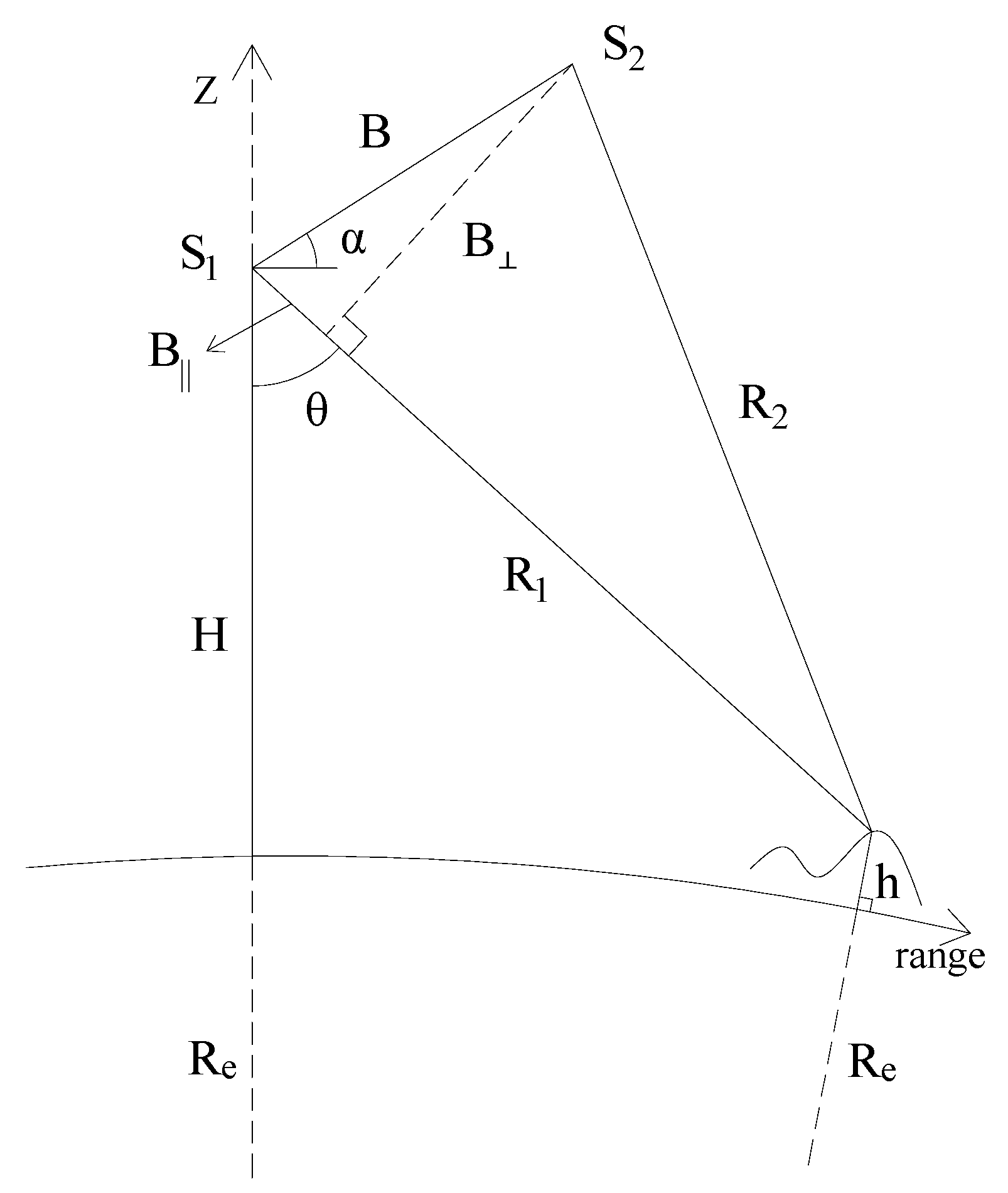
The imaging geometry of an InSAR system is shown in
Figure 1.
and
are the master and slave satellites, respectively,
and
represent the slant range from the master and slave satellite to the scatterer target, respectively,
is the height of the scatterer target,
is the height of the master satellite radar antenna,
is the local radius of the earth,
is the incidence angle,
is the spatial baseline, and
is the baseline inclination. The expression of target height measurement is as follows:
As shown in
Figure 1, the baseline can be decomposed into parallel and perpendicular components along the line of sight (LOS), which are called the parallel baseline
and the perpendicular baseline
, respectively. The relationship can be expressed as follows:
Considering the spaceborne bistatic SAR system, the interferometric phase
can be represented as follows:
where
is the wavelength of the radar system. Because the slant range is much larger than the baseline in a spaceborne SAR system,
can be approximated by the parallel baseline [
15]:
Combining Equations (2) and (4), Equation (1) can be further expressed as follows [
16]:
Uncertainties in each of the parameters
,
,
,
, and
will lead to uncertainties in the height measurement. Therefore, we compute the differential for each individual parameter, and the height estimation error with respect to the estimation error of each parameter can be expressed by Equation (11) under the assumption that the errors are not correlated with each other.
where
and
. Equation (6) shows the allowable accuracy level of the satellite orbit determination uncertainties. The parameter
corresponds to the error of the actual slant range, which is usually caused by SAR system clock-timing uncertainties, sampling clock jitter, propagation delays due to atmospheric and ionospheric effects, etc. Equation (8) places stringent requirements on the system attitude and the determination of the baseline. Comparing the error transfer coefficient of Equations (8) and (9), their ratio is
. Taking the TanDEM-X system parameters as an example, the ratio is always smaller than 1. In other words, the estimation error of baseline inclination will be propagated the height measurement with the greater multiple. Regarding spaceborne SAR systems, due to the azimuthal clock-timing error, it is generally necessary to set ground control points, such as manually placed corner reflectors, to correct the abovementioned errors accurately [
17,
18,
19,
20]. Equation (10) represents the height measurement uncertainty associated with the interferometric phase error, which is mainly caused by the absolute phase offset and several decorrelation factors. The former can also be corrected by ground control points, while the latter is random and cannot be corrected by the above method.
Combining the error characteristics mentioned above, we will concentrate on analyzing the influence of random error, i.e., the interferometric phase error introduced by decorrelation factors, on the elevation measurement accuracy. The parameters , , and are considered known either by the use of precise orbit information or after an adjustment procedure involving ground control points.
3. Optimal Baseline Model
The random interferometric phase errors consist of spatial decorrelation, Doppler decorrelation, volume decorrelation, temporal decorrelation, and decorrelations due to the limit signal-to-noise ratio, quantization, and ambiguities. In this paper, we only consider the spatial decorrelation to investigate the optimal baseline model. Both the geometric systematical error and the decorrelated random error, which affect the phase unwrapping accuracy, are included in this paper.
The spatial decorrelation is mainly affected by the spatial baseline, which can be expressed by the baseline coherence. The baseline coherence is a function of the perpendicular baseline and the critical baseline [
21]:
where
represents the baseline coherence and
represents the critical baseline. The baseline coherence is only related to the perpendicular baseline, which is similar to the relationship between the height measurement error and the phase error described by Equation (10), and neither of them is impacted by the parallel baseline. Therefore, the optimal baseline analysis mentioned in this paper will be directed at the perpendicular baseline to avoid errors introduced by the baseline inclination as much as possible.
When
is greater than
, the spectral shift equals the bandwidth in the range direction, making the signal entirely decorrelated. The critical baseline for the bistatic SAR system can be expressed as follows [
5]:
where
is the slant range,
is the frequency bandwidth of the system,
is the speed of light, and
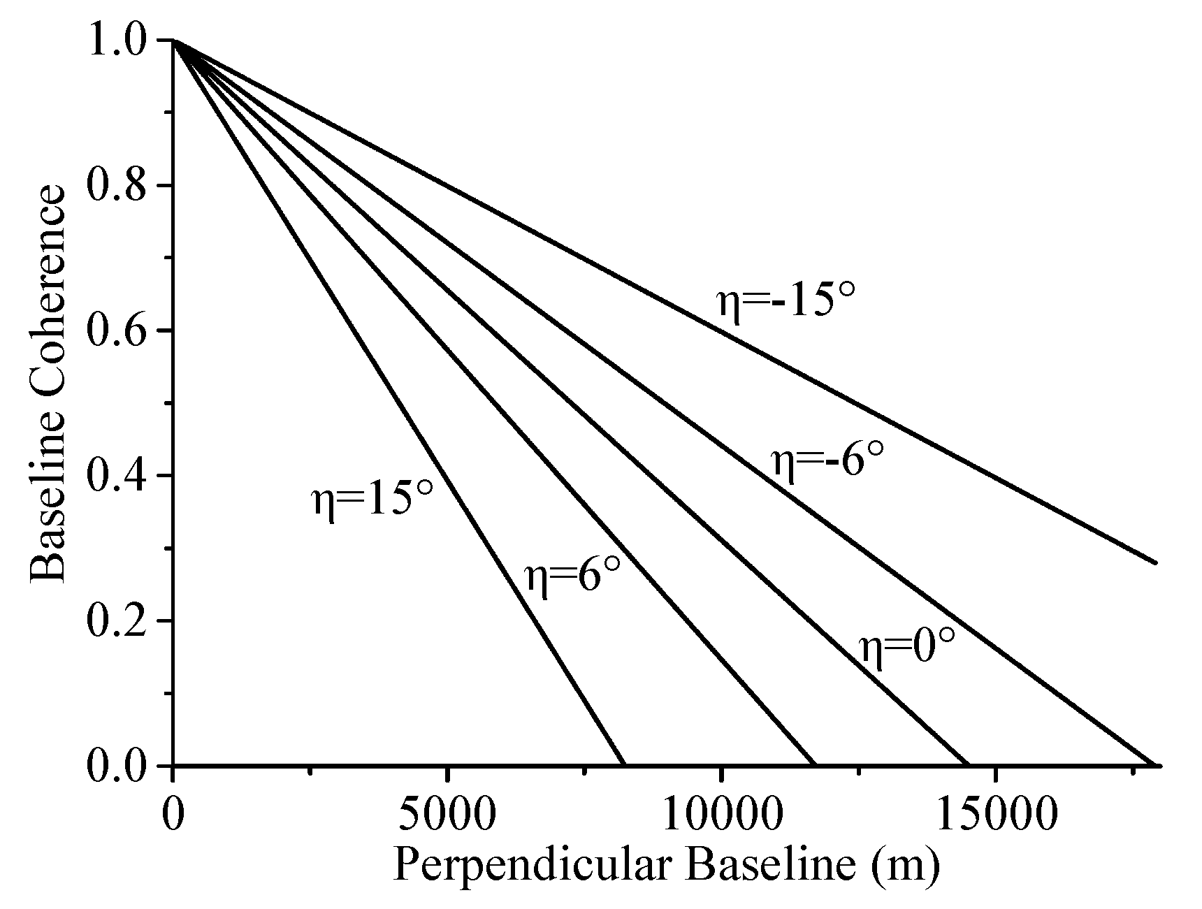
is the local terrain slope. The terrain slope angle is positive when the terrain faces the sensor and vice versa. Taking a TanDEM-X image pair covering Weinan City, Shaanxi Province on September 3, 2013 as an example, the wavelength is 3.2 cm, the slant range is approximately 675 km, the orbital altitude is approximately 514 km, the incidence angle is approximately 42.5°, and the frequency bandwidth is 110 MHz. The relationships among the baseline coherence, the perpendicular baseline, and the terrain slope are shown in
Figure 2.
3.1. Interferogram Simulation
To determine an accurate optimal baseline model, we performed a statistical analysis on the simulated interferometric data based on the bistatic SAR system. First, we simulated the DEM data using a simple terrain slope. Second, the interferometric phase is simulated by calculating the difference in the slant range between the master and slave satellites in the radar coordinate system based on the simulated DEM and the satellite imaging parameters. Then, to properly analyze the relationships among the perpendicular baseline, the terrain slope and the interferometric phase error, the coherence map is simulated only by the spatial decorrelation calculated from geometric imaging parameters. In this paper, the terrain slope is derived according to a simulated DEM with a resolution of 10 m. Finally, we simulate the phase noise based on its relationships with the number of looks and the coherence [
22]:
where
denotes the phase variance,
denotes the correlation coefficient,
indicates the number of looks,
indicates the expectation operator, and
is the probability density function of the interferometric phase and can be calculated as follows:
where
.
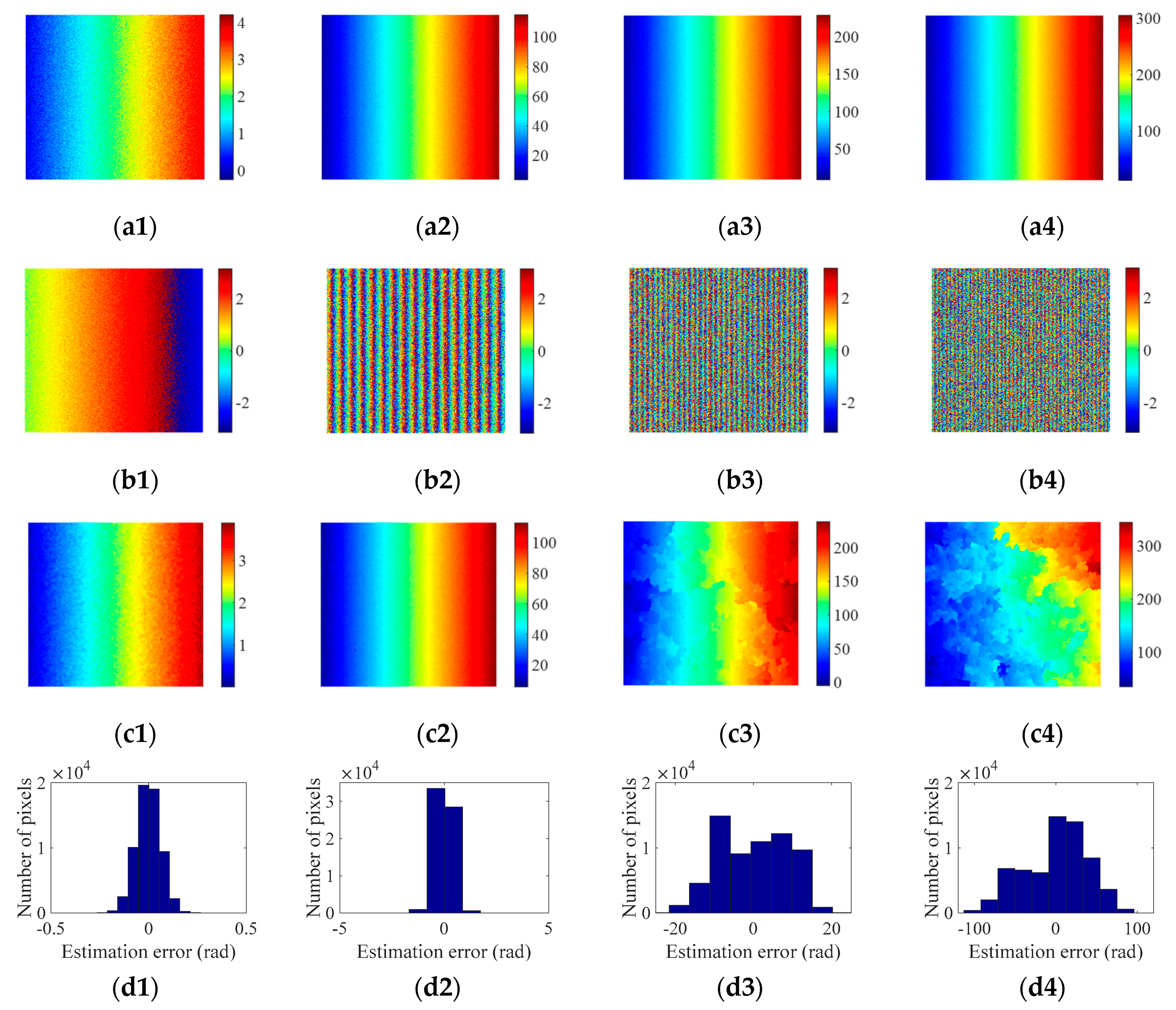
Based on the above formula, this paper simulates the phase noise for
L = 1 and obtains the simulated noisy interferometric phase by adding the phase noise to the true phase and wrapping it. The simulated data sets based on different perpendicular baselines and terrain slopes are shown in
Figure 3.
3.2. Phase Unwrapping Method
As the perpendicular baseline increases, the interferometric fringes produced by the same height change become denser and the phase unwrapping becomes more difficult. Moreover, the interferometric coherence and the accuracy of the unwrapped phase worsen. Therefore, the effectiveness of phase unwrapping during the phase error analysis should be investigated.
Because interferogram filtering would introduce more uncertainty factors, it is not performed. To keep up with the development of phase unwrapping algorithm and ensure a certain success rate of phase unwrapping, this paper adopts an adaptive unscented Kalman filter phase unwrapping method [
13,
14], which is relatively optimal. Compared to traditional phase unwrapping methods, this method that combines an amended matrix pencil model, an adaptive unscented Kalman filter, an efficient quality-guided strategy based on heapsort, and a median filter could achieve more accurate interferometric phase maps. The unwrapped phase and estimation error histograms are shown in
Figure 3.
The estimation error histogram is obtained by simply calculating the difference between the unwrapped phase and the true interferometric phase, which could be more intuitively show the quality of the unwrapping results. However, the interferometric phase error refers to the PUE calculated by the root mean square (RMS) between them. As shown in
Figure 3, as the perpendicular baseline increases, the fringe density of the wrapped interferometric phase increases and the influence of noise on the phase increases, which will weaken the coherence. Correspondingly, the unwrapped phase will worsen. For example, in the case in which the baseline length is 8000 m, the fringes are very dense and the interferometric phase is almost completely covered by noise. In this case, the average estimation error reaches 40 radians, which indicates that the unwrapping method is largely invalid.
3.3. Phase Unwrapping Error Model
To establish an accurate model for the PUE, the perpendicular baseline and the terrain slope, phase simulation and phase unwrapping analyses based on different perpendicular baseline lengths are carried out under a simple terrain with slope angles of approximately 0~8, 10, 12, 14, and 16 degrees. The range of the perpendicular baseline varies between 0 m and the critical baseline, and the step interval is 50 m. Considering the randomness of noise, this paper simulates the same perpendicular baseline length and terrain slope angle 30 times. The mean PUE under the same conditions is fitted as a function of the perpendicular baseline.
In this paper, the Levenberg-Marquardt (LM) [
23,
24,
25] with universal global optimization (UGO) [
26] algorithm is used to optimize the fitting analysis described above for a large amount of simulated data. Considering the complex PUE variation trends, this paper adopts piecewise fitting. The discontinuity points are usually selected at positions after the sudden change in the PUE trend. The partially fitted results are shown in
Figure 4.
When the baseline length is less than approximately 200 m, the PUE increases rapidly as the perpendicular baseline increases. When the perpendicular baseline is between 200 m and 1200 m, the PUE changes slowly, indicating that the phase unwrapping method can effectively resist the decorrelation caused by the baseline in this range. However, the PUE still increases as the perpendicular baseline increases. Subsequently, the dispersion of the PUE increases with changes in the perpendicular baseline, which indicates that the phase unwrapping effectiveness begins to decrease gradually. Accordingly, the PUE curves change rapidly. At this stage, the main reason why phase unwrapping begins to fail is the increase in the fringe density. When the perpendicular baseline length reaches the critical baseline, it theoretically leads to complete decorrelation and the interferometric phase is completely covered by the stochastically distributed phase error. Thus, the unwrapped phase should be completely contaminated by the noise error. In this case, the additional noise from Equations (13) and (14) reaches its maximum value. Additionally, the unwrapping method is almost completely invalid as the length approaches the critical baseline. Thus, as the baseline is approached, the PUE would reach a saturated state; that is, the PUE tends to stabilize or decelerate the growth rate. As shown in
Figure 4j, when
, although the baseline does not reach the critical baseline, the phase unwrapping is largely invalid due to excessively dense fringes; therefore, PUE saturation occurs early. This phenomenon occurs only when the baseline reaches at least approximately half of the critical baseline length, which is far greater than the optimal baseline and will not affect the subsequent optimal baseline analysis.
Moreover, if the perpendicular baseline length is held constant, the PUE increases with increasing terrain slope angle. On one hand, the critical baseline and coherence would decrease in this case as described by
Figure 2. On the other hand, with an increasing slope angle, the height difference gradually increases under the same image size and DEM resolution; that is, the phase gradient gradually increases. Therefore, the fringe density of the interferogram gradually increases, resulting in an increase in the PUE.
3.4. Optimal Baseline Analysis
According to
Section 2, as the perpendicular baseline increases, the sensitivity of the interferometric phase to the height changes will increase. This sensitivity can be described by the height ambiguity, i.e., the height difference corresponding to a
phase shift:
where
represents the height ambiguity. Considering the terrain slope, it can be further expressed as follows:
In addition, as described in
Section 3.3, the PUE will increase with an increasing perpendicular baseline, and the height measurement accuracy will worsen. Therefore, there exists an optimal baseline range for the height measurement. Without considering climatic and environmental influences, the optimal baseline is defined as the perpendicular baseline, which minimizes the standard deviation of the target height estimation. Considering the above analysis and ignoring some systematic influencing factors, the standard deviation of height can be described by Equation (18) below. Note that
; therefore,
k can be regarded as a constant.
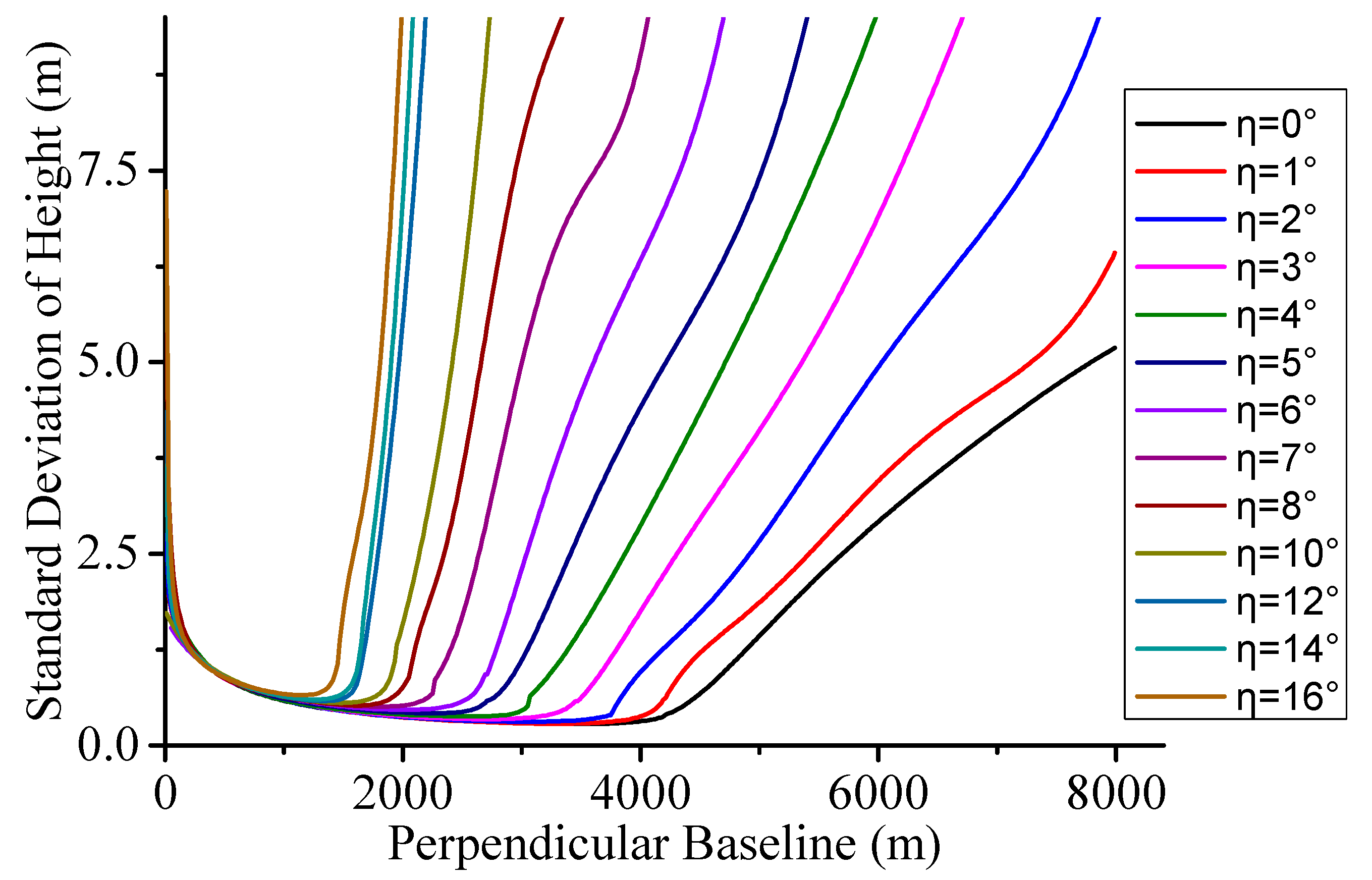
Based on the PUE model described in
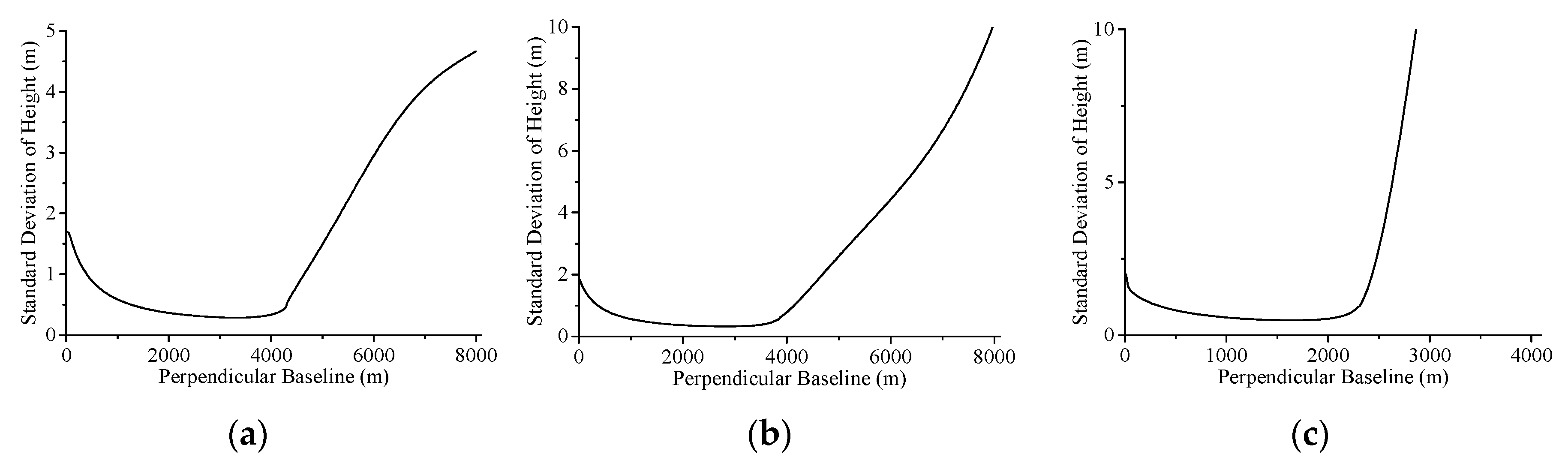
Section 3.3, the standard deviation of height from different terrain slope angles can be calculated by Equation (18). To observe the relationships among the height error, the perpendicular baseline and the terrain slope more intuitively, a small height error is only selected for mapping as shown in
Figure 5.
As shown in
Figure 5, the height error is inversely proportional to the perpendicular baseline when the baseline length is less than approximately 1000 m. In this case, the PUE is very small and the height error is mainly determined by the height ambiguity. However, as the baseline length reaches a critical value, the height error will increase rapidly. At this time, the height error is mainly affected by the PUE because the phase unwrapping method is beginning to fail. Combined with the PUE curves shown in
Figure 4a, the critical value is usually located at a position similar to that of the sudden change points on the PUE curves. Obviously, the critical value will increase with a decreasing slope angle, which also means that the optimal baseline range will increase. In fact, the height error will be very large when the baseline length is close to zero or the critical baseline. Nevertheless, because the PUE will reach a saturated state when the baseline approaches the critical baseline, the height error will be affected and gradually stabilize. To more intuitively analyze the variation in the height error around the optimum baseline range, the corresponding transverse and longitudinal axes are shortened here. Therefore, the saturation phenomenon mentioned above is not shown. For different terrain slopes, the optimal baselines that minimize the standard deviation of height are shown in
Table 1.
As described in
Table 1, although the optimal baseline varies with the terrain slope, the corresponding optimal baseline coherences are essentially equal in the cases of
or
at approximately 0.764 or 0.853, respectively. In other cases, the change in the optimal baseline coherence is approximately linear. Combined with
Figure 5, we can extend the optimal baseline coherence range appropriately, and the empirical model is expressed as follows:
Thus, the optimal baseline range can be obtained from Equation (12) based on the optimal baseline coherence model, which can be expressed as follows:
Similarly, we also experimentally analyzed the optimal baseline variation for negative slope angles. As described in
Table 2, the variation in the optimal baseline coherence is largely consistent with that of the positive slope angle. Specifically, as
and
, the optimal baseline coherence increases slowly with an increase in
; and as
, it increases rapidly. When the absolute value of the terrain slope angle is the same, the optimal baseline of the negative slope is always larger than that of the positive slope because of the incidence angle. However, when the baseline is relatively large, the main influencing factor of the PUE is the fringe density; therefore, the increment in the optimal baseline is not very large. However, the increment in the critical baseline is much larger than that of the optimal baseline, which results in an inconsistent optimal baseline coherence and a larger growth rate than the positive slope.
However, in actual topographic mapping, there is not a fixed optimal baseline parameter because of the complexity of the terrain. Therefore, the optimal baseline selection can only be made according to the distribution of the topographic gradient to minimize the average height measurement error in the surveyed area.
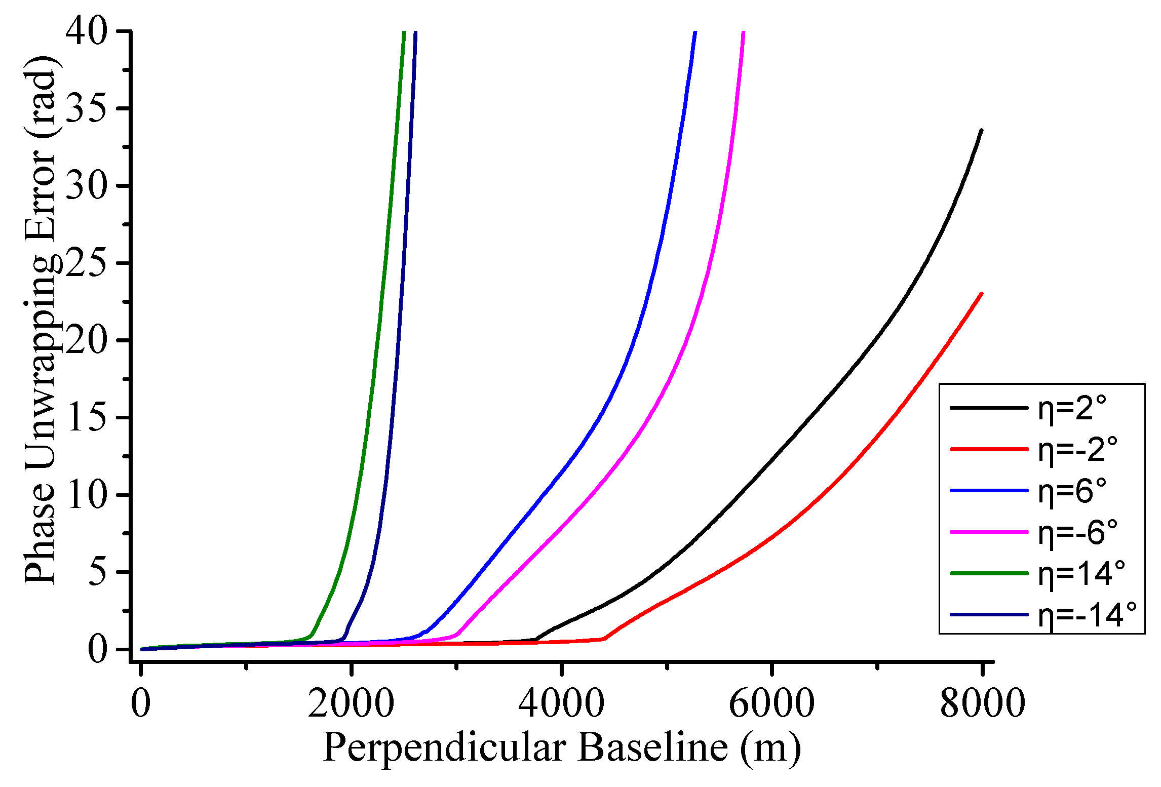
In fact, the positive and negative slope angles of the actual terrain always correspond. According to
Figure 6, which compares the PUEs of different positive and negative terrain slopes, before the sudden change in the PUE curves, the PUEs for positive angles are basically consistent with the PUEs for negative angles. However, when the terrain slopes have the same absolute value, the baseline length at the rapidly changing position of the PUE corresponding to the negative slope angle is larger than that of the positive slope angle. Therefore, the influence of the PUE corresponding to the positive slope pixels on the whole PUE is higher than that of the negative slope pixels. Moreover, the PUEs corresponding to negative slopes may have a greater impact overall than that of the small terrain slopes. Thus, the absolute value of the terrain slope angle will be used to analyze the distribution of the topographic gradient. Then, the average slope angle of the complex terrain can be obtained and the optimal baseline range can be further calculated by Equations (18) and (19).
4. Experimental Analysis
To evaluate the optimal baseline model described in
Section 3.4, this paper uses a complex terrain for the experimental analysis and the parameters of the SAR system that are employed are the same as above. Moreover, to increase the simulated complex terrain's similarity to the real terrain, the terrain was divided into two categories: uniformly and nonuniformly distributed positive and negative slope angles, where the mean values of the positive and negative slope angles in the determined study area are close to or deviate from 0. Finally, the optimal baseline ranges of different terrain types are given for reference.
4.1. Uniform Distribution of Positive and Negative Slope Angles
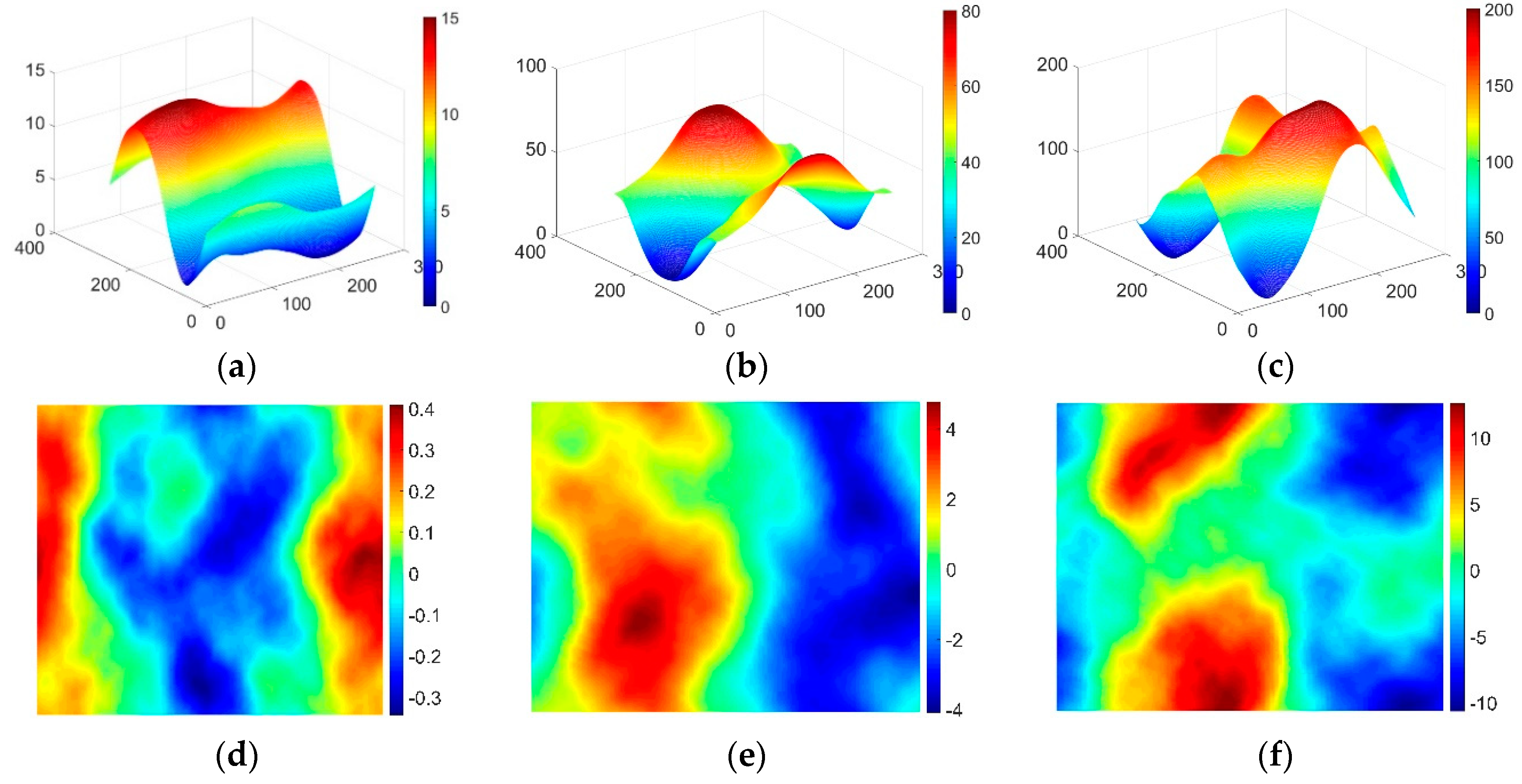
For the case of a relatively uniform distribution of positive and negative slope angles, three kinds of complex terrains with slope angles ranging from small to large are successfully simulated in this paper. The simulated DEM with a size of 256 (range) × 256 (azimuth) pixels and the terrain slope of every pixel calculated by the DEM resolution are shown in
Figure 7.
As shown in
Figure 7, the slope angles of the simulated complex terrain are approximately uniform and the average calculated values are approximately −0.005, −0.018, and 0.262 degrees in
Figure 7d–f, respectively; however, the range of the slope is obviously different, and the intervals are approximately (−0.34, 0.41), (−4.08, 4.76) and (−10.64, 12.56), respectively.
Combined with the optimal baseline model, it is necessary to determine an appropriate slope angle to calculate the optimal baseline range. As described in
Section 3.4, for positive and negative slopes with the same absolute value, the influence of the negative slope angle pixels on the overall PUE is smaller than that of positive slope angle pixels. Thus, the absolute value of the negative slope angle will be used when calculating the average slope angle of a complex terrain. Nevertheless, it is still inappropriate to calculate the arithmetic mean of the absolute value of the slope angle. As shown in
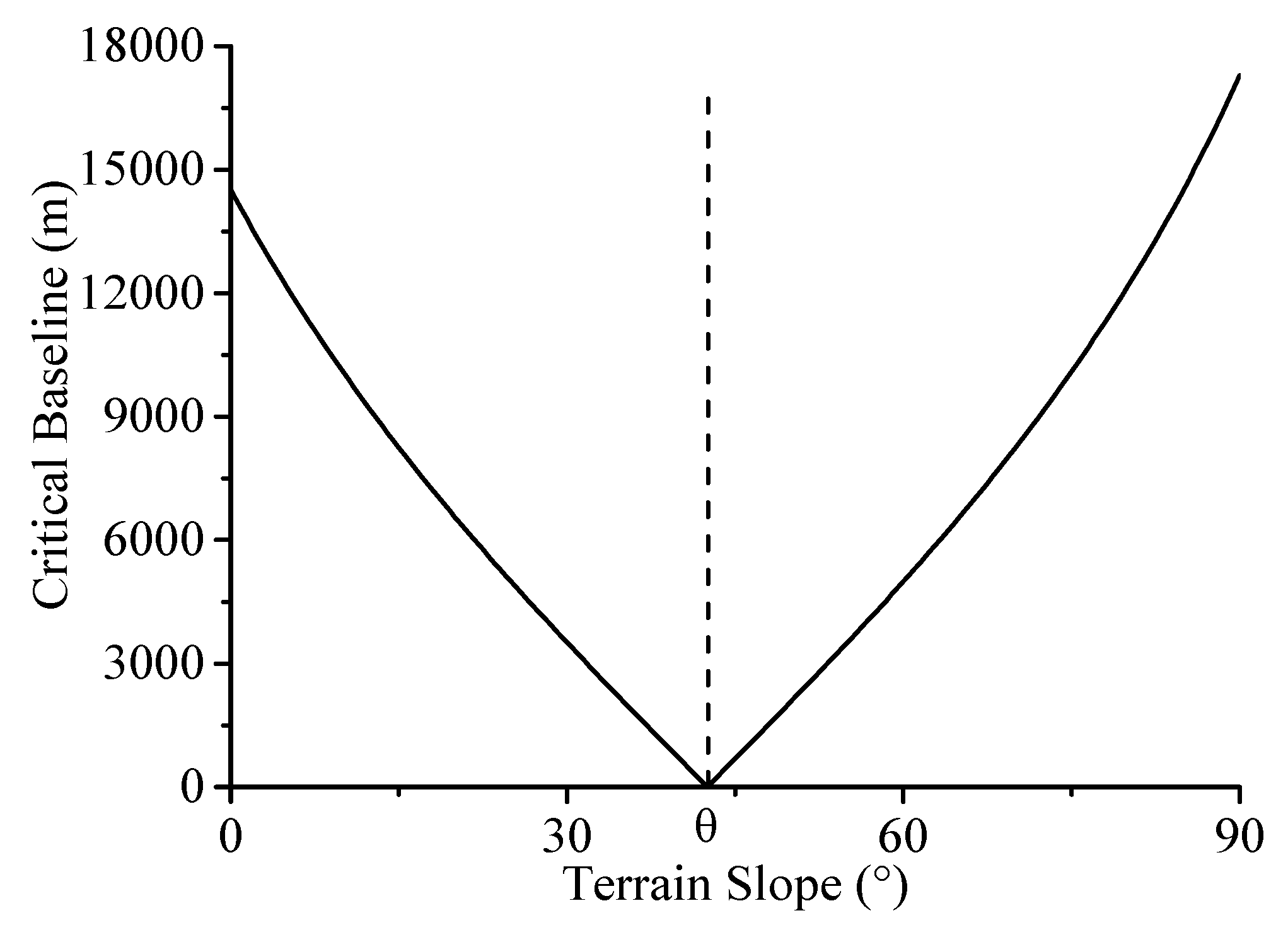
Figure 4a, under the same perpendicular baseline, the influence of the terrain slope on the PUE will increase with an increasing slope angle. However, the above analysis is only based on the condition that the terrain slope angle is smaller than the incidence angle. If the terrain slope angle is larger than the incidence angle, then the opposite is true. In theory, the PUE is inversely proportional to the baseline coherence and the baseline coherence is proportional to the critical baseline. Therefore, the PUE is inversely proportional to the critical baseline. The relationship between the critical baseline and the terrain slope angle is shown in
Figure 8.
Thus, the PUE will be proportional to the terrain slope if the slope angle is smaller than the incidence angle; otherwise, it will be inversely proportional to the terrain slope.
Based on the above conclusion, we propose a weighted average method to calculate the average slope angle of a complex terrain. First, the absolute value of the slope angle is divided into several intervals with 0.5 degree steps. Then, the arithmetic mean of each interval is calculated separately. Finally, the mean value of each interval is weighted to obtain the final average terrain slope angle.
where
represents the final average slope angle of a complex terrain,
represents the number of intervals divided by steps of
,
refers to the arithmetic mean of the slope angle in each interval,
denotes the number of pixels in each interval, and
denotes the weight corresponding to each interval. The weight is defined as follows:
Certainly, if the number of pixels in the interval is small, the interval may be ignored; otherwise, the final average slope angle of a complex terrain will be overestimated.
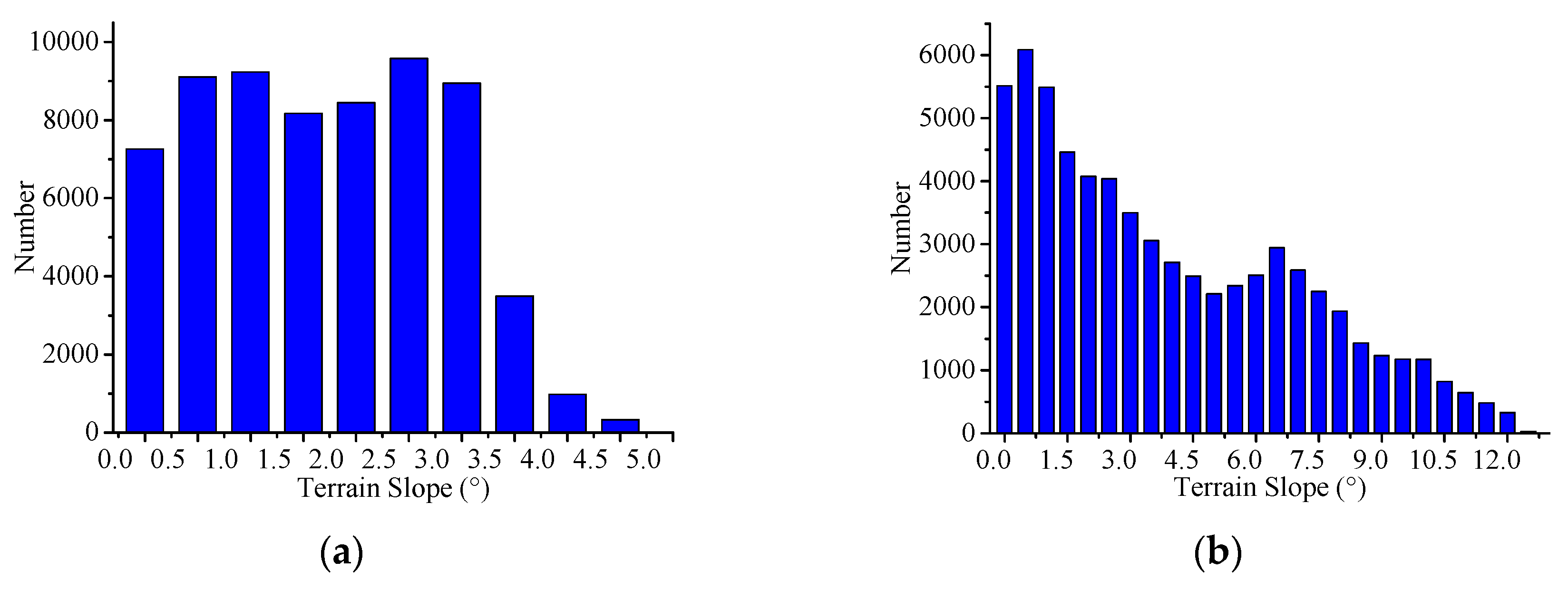
According to the above analysis, the terrain slope maps from
Figure 7 can be divided into interval histograms with 0.5 degree steps shown in
Figure 9. Since the maximum slope shown in
Figure 7d is less than the step interval, it can only be divided into one interval and its weighted average is equal to the arithmetic average of the absolute values of slope angles. Therefore, the interval histogram corresponding to
Figure 7d will not be shown.
In this paper, based on the simulated image size, the total number of pixels is 65536. We assume that the interval of the number of pixels less than 500 (approximately less than 1% of the total number) can be ignored. Therefore, the intervals of slope angles larger than 4.5 degrees and 11.5 degrees will not participate in the weighting operation. According to Equation (21), the final average slope of the complex terrain corresponding to
Figure 7a–c is 0.15, 2.90 and 7.58 degrees, respectively. Combining the optimal baseline model as described in
Section 3.4, the optimal baseline ranges can be calculated as follows:
,
and
.
To evaluate the validity of the optimal baseline model, the data fitting method described in
Section 3.3 is again used to fit the PUE curve of the complex terrain shown in
Figure 7. The final height measurement error maps associated with the perpendicular baseline are obtained as shown in
Figure 10.
Similarly, to show the optimal baseline range more intuitively when the standard deviation of height is small, only a segment of the standard deviation of height is presented in
Figure 10. From
Figure 10a–c, the obtained optimal baselines are 3308 m, 2817 m and 1650 m, respectively. These values are all within the optimal baseline range estimated by the optimal baseline model, and the estimated optimal range is consistent with the optimal baseline range obtained by
Figure 10. Thus, the validity of the model is verified.
4.2. Nonuniform Distribution of Positive and Negative Slope Angles
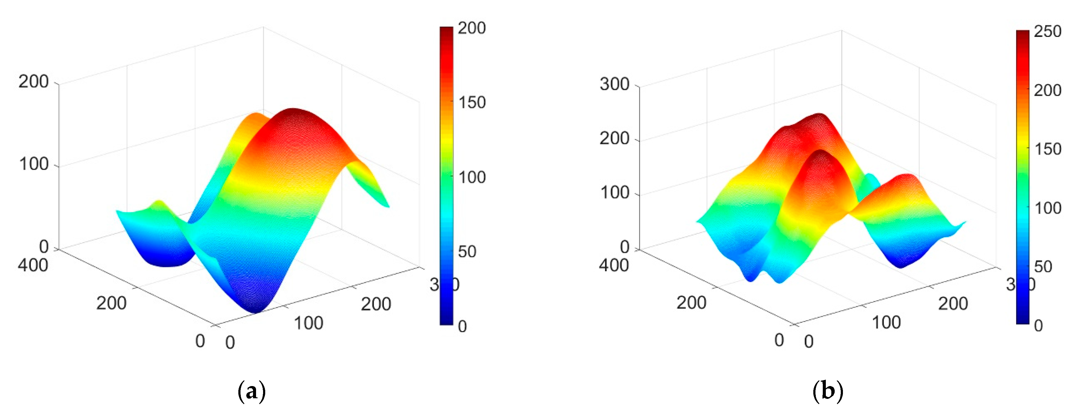
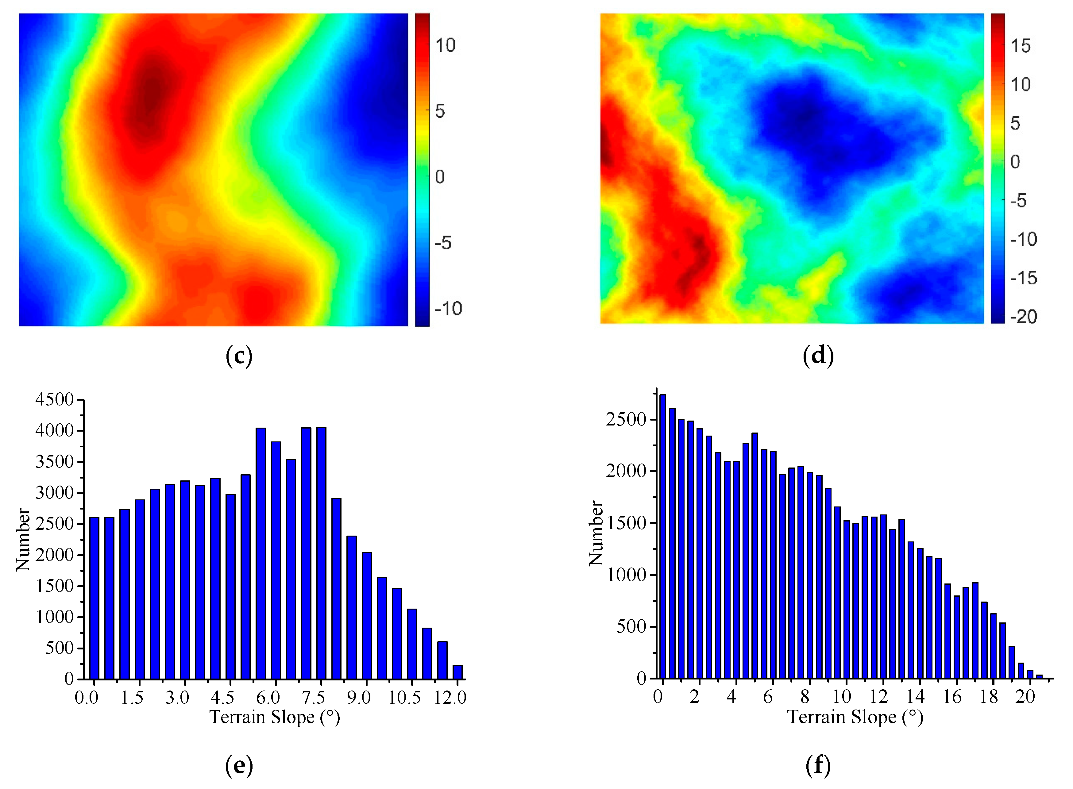
To comprehensively consider the changes in the complex terrain and further evaluate the reliability of the optimal baseline model, two sets of irregular DEMs with sizes of 256 (range) × 256 (azimuth) pixels are simulated. In addition, the positive and negative terrain slopes will be nonuniformly distributed.
Figure 11a,b are two sets of simulated DEMs for different complex terrains, and
Figure 11c,d are the corresponding terrain slope angle distribution maps calculated by the DEM resolution and the SAR system parameters. A positive slope angle accounts for a large proportion of the first study area as shown in
Figure 11c, whereas a negative slope angle dominates the second study area as shown in
Figure 11d. The arithmetic average of slope angle in the complex terrains is approximately 1.13 and −3.26 degrees. Considering that the number of pixels in each slope angle interval should be larger than 500, the intervals greater than 12 and 19 degrees corresponding to
Figure 11e,f, respectively, will be discarded. With the proposed weighted average method, the final average slope angles of the complex terrain corresponding to
Figure 11a,b are approximately 7.91 and 12.58 degrees, respectively. The optimal baseline coherence calculated by Equation (19) are
and
. Then, the estimated optimal baseline ranges are
and
.
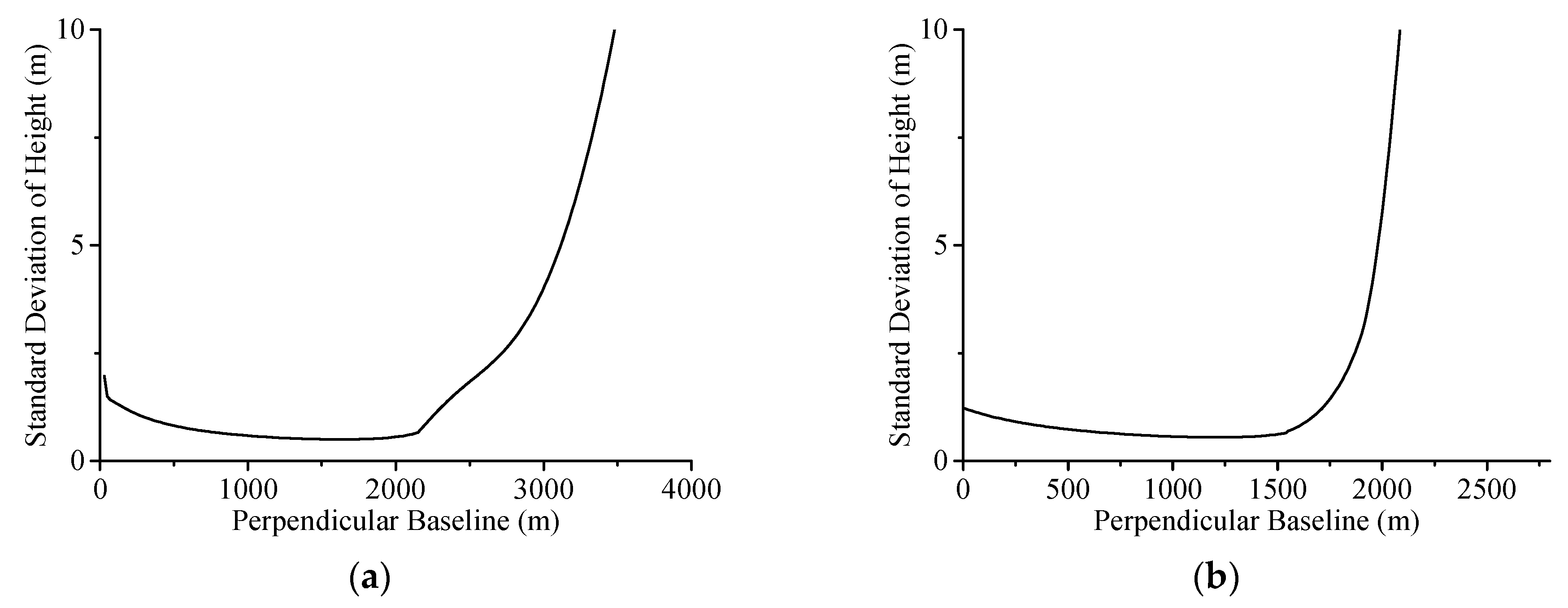
Similar to the experimental analysis in
Section 3, the interferometric phase simulation and the data processing analysis are performed for the above complex terrains. The PUE under different perpendicular baselines are fitted and analyzed, and the final height error maps are obtained and shown in
Figure 12a,b.
For the abovementioned complex terrains, the optimal baselines are 1632 m and 1214 m. Obviously, they are both within the optimal baseline ranges estimated by the proposed optimal baseline model. Thus, the validity and reliability of the optimal baseline model in this paper are further verified. Moreover, the feasibility of the weighted average method, which is based on the absolute value of terrain slope, is also verified even when the positive and negative slope angles are relatively nonuniform in the study area.
4.3. Optimal Baseline Range for Different Terrain Types
Combined with
Section 4.1 and
Section 4.2, the reliability of the optimal baseline model proposed in this paper has been verified under the different slope ranges, such as (−0.34, 0.41), (−4.08, 4.76), (−10.64, 12.56), (−11.44, 12.34) and (−21.03, 18.99), which correspond to average slopes of 0.15, 2.90, 7.58, 7.91 and 12.58 degrees, respectively. Meanwhile, the validity of the weighted average method to calculate the average slope angles of complex terrain is also verified. Combining the definition of terrain types [
27], the optimal baseline range could be derived for reference based on the slope ranges of the different terrain types shown in
Table 3. Other terrain types except that of the Alpine region have been analyzed by the above experiments.
Furthermore, according to
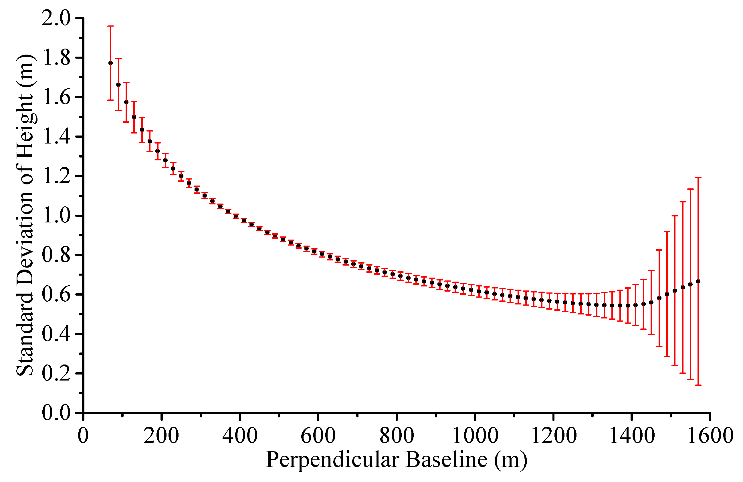
Figure 5, although the height measurement accuracy corresponding to different terrain slope is not optimal when the baseline is less than 1500 m, the height measurement accuracy is relatively stable during this period. The detailed variation of the height measurement accuracy at different terrain slope during this period is shown in
Figure 13. It can be found that the height measurement accuracy is stable, i.e. the height measurement accuracy of different terrain slope is basically the same and the standard deviation of height measurement errors at different terrain slope are all less than 0.1m, during the baseline range from 100 m to 1400 m. Maybe, for the SAR system with immutable baseline or small baseline variability, this baseline range will be more valuable for reference to better adapt to the observation of different terrain slope.
5. Discussion
In this study, the optimal baseline based on a spaceborne bistatic SAR system was modeled. Compared with the previous model [
3,
7], it considered the influence of the perpendicular baseline, the terrain slope and the unwrapping effectiveness on the PUE, and a reasonable weighted average algorithm was proposed to calculate the average slope of a complex terrain. This model is of great significance for the design of subsequent spaceborne bistatic SAR systems and the acquisition of high-precision DEMs for certain topographies.
However, this paper only considered the spatial decorrelation in the PUE model, and the Doppler decorrelation, volume decorrelation, temporal decorrelation and decorrelations caused by the limit signal-to-noise ratio, quantization, and ambiguities were ignored. Thus, the actual optimal coherence can be expected to be less than the estimated optimal baseline coherence, and the optimal baseline range can be expected to be larger than the estimated optimal baseline range. In practical applications, based on the estimator, slight adjustments could be made to the optimal coherence range to reduce the influence of other types of decorrelation. Further studies of the influence of other coherence values are necessary to obtain an accurate optimal baseline range. In addition, to suppress the related unwrapping error, this paper chose the adaptive unscented Kalman filter phase unwrapping algorithm [
13,
14], which is superior to the traditional phase unwrapping methods. In future research, a better processing method will be selected to obtain a higher-precision DEM; therefore, choosing a better phase unwrapping algorithm for experimental analysis in this paper will be more conducive to follow-up research.
Moreover, in the experimental analysis of the
Figure 11b data set, although the number of pixels in the intervals of slopes larger than 19 degrees is small, the maximum value of the slope angle reaches 21 degrees, which will also impact the overall PUE. Thus, when the range of the absolute value of the slope angle is large, the average slope may be underestimated due to the abandonment of more intervals. This phenomenon is also the reason why the actual optimal baseline obtained by the experiment is close to the lower limit of the estimated optimal baseline range. Therefore, to avoid this phenomenon, the threshold should be appropriately reduced according to the actual complex terrain. For example, we could set the threshold to 400; i.e., intervals for fewer than 400 pixels will be ignored.
6. Conclusions
In this study, we analyzed the influences of SAR system parameters, such as the positioning system of the satellite platform, the slant range, the baseline length, the baseline inclination, and the interferometric phase error, on the accuracy of height measurement from a spaceborne bistatic SAR system. Because the interferometric phase error introduced by several decorrelation factors is random, it cannot be corrected by the ground control points. Thus, the PUE, which is mainly influenced by the perpendicular baseline, the terrain slope and the unwrapping effectiveness, is modeled based on a simple terrain, and the standard deviation of height is calculated. Then, the optimal baseline model that maximizes the height measurement accuracy is obtained. Combined with the PUE model, a weighted average method is also proposed to calculate the average slope angle of the complex terrain. Finally, the validity and reliability of the optimal baseline model are confirmed by considering the uniform and nonuniform distributions of positive and negative slope angles and the variation in slope angle on the complex terrain. In addition, the optimal baseline ranges of different terrain types are given for reference.


