Vegetation Phenological Changes in Multiple Landforms and Responses to Climate Change


1
School of Geography and Tourism, Shaanxi Normal University, Xi’an 710119, China
2
China Academy of Space Technology-Xi’an, Xi’an 710000, China
3
National Demonstration Center for Experimental Geography Education, Shaanxi Normal University, Xi’an 710119, China
*
Author to whom correspondence should be addressed.
ISPRS Int. J. Geo-Inf. 2020, 9(2), 111; https://0-doi-org.brum.beds.ac.uk/10.3390/ijgi9020111
Submission received: 16 December 2019
/
Revised: 14 February 2020
/
Accepted: 17 February 2020
/
Published: 19 February 2020
Abstract
:Vegetation phenology is highly sensitive to climate change, and the phenological responses of vegetation to climate factors vary over time and space. Research on the vegetation phenology in different climatic regimes will help clarify the key factors affecting vegetation changes. In this paper, based on a time-series reconstruction of Moderate-Resolution Imaging Spectroradiometer (MODIS) normalized difference vegetation index (NDVI) data using the Savitzky–Golay filtering method, the phenology parameters of vegetation were extracted, and the Spatio-temporal changes from 2001 to 2016 were analyzed. Moreover, the response characteristics of the vegetation phenology to climate changes, such as changes in temperature, precipitation, and sunshine hours, were discussed. The results showed that the responses of vegetation phenology to climatic factors varied within different climatic regimes and that the Spatio-temporal responses were primarily controlled by the local climatic and topographic conditions. The following were the three key findings. (1) The start of the growing season (SOS) has a regular variation with the latitude, and that in the north is later than that in the south. (2) In arid areas in the north, the SOS is mainly affected by the temperature, and the end of the growing season (EOS) is affected by precipitation, while in humid areas in the south, the SOS is mainly affected by precipitation, and the EOS is affected by the temperature. (3) Human activities play an important role in vegetation phenology changes. These findings would help predict and evaluate the stability of different ecosystems.
1. Introduction
Phenology is the study of seasonally recurring plant and animal life cycle stages or phenophases, such as the leafing and flowering of plants, the maturation of agricultural crops, the emergence of insects, and the migration of birds [1]. Phenology is considered the pulse of our planet (www.usanpn.org). The International Biological Program (IBP) defined phenology as a recurring event that our ancestors used to guide agricultural production for thousands of years [2]. Phenology can reflect the climate and environmental changes and is an important indicator of changes in the natural environment [3,4]. Moreover, plants are an important part of the ecosystem, providing the main portions of matter and energy [5]. Phenology plays a crucial role in the carbon balance of terrestrial ecosystems [6]. Therefore, it is very important to study vegetation phenology. A change in vegetation phenology has many consequences for ecological processes, agriculture, forestry, human health, and the global economy [7]. Elucidating the trends of vegetation phenology can improve our understanding of the impacts of climate change on ecosystem productivity and carbon cycling and the associated feedback to the climate [8].
In recent decades, warming increasing trends and frequent extreme events due to climate changes have produced significant impacts on many ecosystems and changed the vegetation phenology [9,10]. Vegetation phenology is very sensitive to climate change, and it is regarded as an important indicator of climate change [11,12,13,14,15]. Various biotic and abiotic factors influence vegetation phenology, including the temperature, photoperiod, precipitation/moisture, vegetation composition, and climate changes [16,17,18,19,20]. In a study conducted in 21 European countries, Menzel et al. found that leaf-on conditions arrived 2.5 days earlier and that leaf-off conditions were delayed by 1 day for every 1°C increase in the temperature, respectively [21]. In the northern hemisphere, spring temperatures were found to have the highest correlation with the start of the growing season (SOS) [22,23,24]. Evidence of the effects of precipitation, nutrients, and soil physical properties on the spring phenology is scarce, and where effects have been found, the effects are small relative to the effect of the temperature in England [25]. However, as research develops, the temperature has been found to not be the only limiting factor of vegetation phenology [26]. Precipitation is also an important factor affecting changes in vegetation phenology [27]. Precipitation during winter and spring has also been found to affect the spring phenology in a complex manner in middle and high latitudes in the Northern Hemisphere [28,29,30]. Solar radiation (the total insolation, peak irradiance, and photoperiod) has also been implicated as a major cue, affecting the phenology in both seasonal and aseasonal periods [31,32]. In some temperate tree species, the photoperiod and winter chilling requirements are also known to play a role in the spring phenology [11]. In addition, studies have suggested that elevated CO2 levels can enhance leaf longevity and impact the vegetation phenology in autumn [33].
Climate changes may accelerate in the future, so there is an urgent need to understand the Spatio-temporal phenological driving forces behind these changes [34]. Advances in remote-sensing technology have greatly expanded the capability of phenology observation [5]. The greenness index has been widely used in vegetation phenology research around the world, and it is retrieved from various satellite remote-sensing data, such as the normalized difference vegetation index (NDVI) [35]. Piao et al. used the method of the greatest increase in the NDVI to extract vegetation phenological parameters in temperate regions of China [36]. The phenological changes in the northern hemisphere over the past 30 years have been discussed by the maximum ratio method [3]. The method of the maximum curvature change has been used to estimate the autumn phenology, which is suitable for the comparison of ground observation data with Moderate-Resolution Imaging Spectroradiometer (MODIS) NDVI data [37]. However, at present, most phenological studies are focused on plateaus, watersheds, forests, and other large-scale spaces [38,39,40,41,42]. There are few studies on the response mechanisms of the vegetation phenology to climate changes under different climatic conditions at medium and small scales. Furthermore, the phenological sensitivity to climate changes across all taxa and scales is different, and there is potential ecological asynchrony [43]. Due to differences in topography and geomorphology, unique regional microclimates are formed, and local models of vegetation phenology arise [37]. We expect that even in areas with similar geographical locations, different local topographical conditions would have a significant impact on the vegetation phenology. The main purpose of this study was to address the following questions:
- (1)
- What is the Spatio-temporal variation pattern of the vegetation phenology?
- (2)
- How do climatic factors, such as temperature, precipitation, and light, affect phenological changes?
Clarifying these issues would help predict and evaluate the stability of different ecological communities and provide an important scientific basis for local sustainable development.
2. Data and Methods
2.1. Study Area
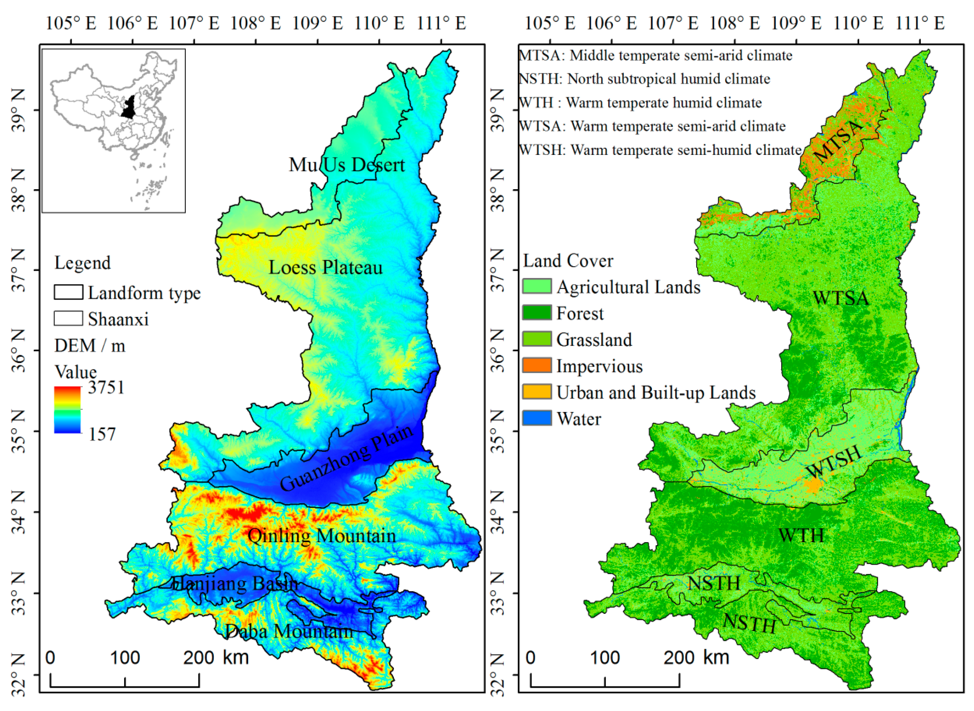
Shaanxi Province (Figure 1) is located at the junction of the eastern humid area and western arid area in China, and its area is approximately 205,600 km². The climate differs from north to south, and the landforms are composed of plateaus, mountains, plains, and basins. According to the landform types, the province can be divided into six parts: the Mu Us Desert (MUD), Loess Plateau (LP), Guanzhong Plain (GZP), Qinling Mountains (QLM), Hanjiang Basin (HJB), and Daba Mountains (DBM) [44]. The only desert landform is a MUD, where the climate is dry and cold, and the vegetation types are mainly desert vegetation, such as Artemisia and Salix. In recent years, the ecological environment has changed due to the Grain for Green Program. The LP is the frailest ecological area, where Yellow River is divided into numerous small tributaries, and the vegetation types are mainly grassland and shrub. The GZP is the largest plain and grain-producing zone, and its vegetation types are mixed deciduous forests and crops. The highest-elevation zone is the QLM, which is predominantly forested, with abundant animal and plant species. The HJB is the source of the HanJiang River, where the vegetation types are broad-leaved forests and crops. There are many mountain ravines crisscrossing the DBM, where the district basically consists of evergreen broad-leaved forests and evergreen deciduous forests.
2.2. Data Source and Preprocessing
2.2.1. NDVI
This paper used MODIS normalized difference vegetation index (NDVI) data as the basic data for the production of remote-sensing vegetation phenology analyses. The NDVI with a 16-day temporal resolution and a 250-m spatial resolution (MOD13Q1, collection v006) was obtained from the Level-1 and Atmosphere Archive & Distribution System (LAADS) Distributed Active Archive Center (DAAC) website (https://ladsweb.modaps.eosdis.nasa.gov/), and two tiles (h26v05 and h27v05) covered the study area. The sixteen-year period between 2001 and 2016 was used. After we obtained the data, we extracted, mosaicked, reformatted, and reprojected the NDVI and pixel-reliability data layer using the MODIS projection tool (MRT) provided by the Land Processes Distributed Active Archive Center (LP DAAC). Subsequently, according to the methods in (SONG Chun-qiao 2011) [45], the pixel-reliability was used to process the NDVI data to improve reliability. In detail, for the same one-pixel position, NDVI values with pixel-reliability values of 0 and 1 were weighted with 1 and 0.8, respectively, and pixels with pixel-reliability data of 2 and 3 were weighted with 0.2. We performed this process in Matlab and marked the NDVI processed according to the pixel-reliability data as the pNDVI (Figure 2).
2.2.2. Meteorological Data
The meteorological data used in this study included the monthly mean temperature, monthly precipitation, and monthly sunshine hours. These data were calculated from the daily values, which were obtained from the Chinese ground meteorological data daily dataset (V3.0) downloaded from the China Meteorological Data website (http://cdc.cma.gov.cn/). The meteorological data were averaged monthly or summed after spatial interpolation using the inverse distance-weighted (IDW) method in ArcGIS, and Spatio-temporal meteorological data at the monthly time scale with a 250-m resolution were obtained covering 2001 to 2016.
2.2.3. Topographic Data
Because there are many landform types in the study area (Figure 1) and due to the altitudinal differences between different landform types, the relationship between the altitude and phenology was analyzed using digital elevation model (DEM) data with a 30-m spatial resolution to explore the influence of the altitude on phenological parameters. The DEM data were derived from the ASTER GDEM V2 dataset, which was downloaded from the Geospatial Data Cloud (http://www.gscloud.cn) of the Computer Network Information Center, Chinese Academy of Sciences. In ArcMap, the DEM data were obtained in separate tiles, which were subsequently mosaicked, resampled to 250 m, and then subset to Shaanxi Province (study area).
Land use data with a 30-m spatial resolution from the Resources and Environment Scientific Data Center, Chinese Academy of Sciences, were used to extract the NDVI in areas with vegetation coverage in the study area by resampling and masking in ArcMap. Pixels with NDVI<0.05 were eliminated to ensure that each NDVI pixel had vegetation cover.
2.3. Remote-Sensing Vegetation Phenology Extraction
2.3.1. Reconstruction of the Vegetation Index Time Series Curve
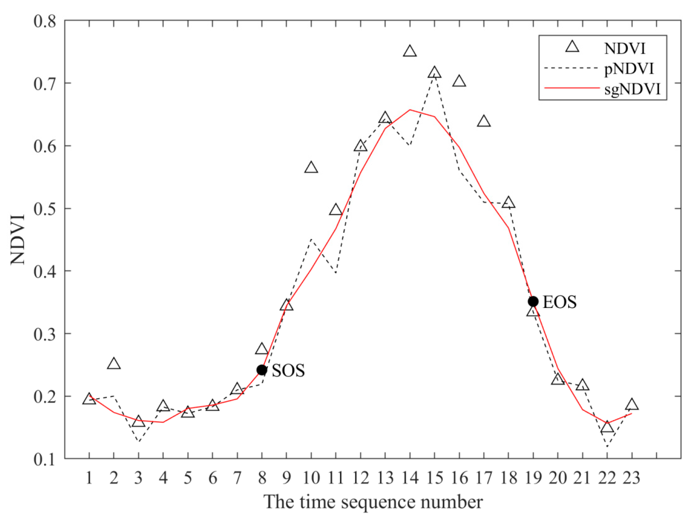
The time series curve of the vegetation index (Figure 2) reflects the growth of vegetation and is the basis for extracting the parameters necessary to assess the vegetation phenology via remote sensing. The NDVI values from the same year were layer-stacked in ArcGIS to obtain multi-band images of 23 periods in that year, with each band representing the NDVI for a certain period, and then the multi-band images were read as a multi-dimensional matrix in Matlab, pixel by pixel. Subsequently, the multi-dimensional matrix was converted into a 1-dimensional sequence to obtain the NDVI time series of the pixel, as shown in Figure 2 NDVI. However, the original NDVI time series curve (Figure 2, NDVI) is uneven and abrupt due to interference from poor atmospheric conditions, clouds, and other unfavorable factors [46], and it is not suitable for use in the direct extraction of vegetation phenological parameters. Therefore, the Savitzky–Golay (S-G) filtering method was used to reconstruct the time series curve before extracting the vegetation phenological parameters.
The S-G filtering method was proposed by Savitzky and Golay in 1964 and is a weighted fitting algorithm for moving windows. The weight coefficients are derived by the least-squares fitting of a given high-order polynomial within the moving window [47]. Therefore, during the process of smoothing and denoising the NDVI time-series data with the S-G filter, the establishment of two parameters is crucial. The first parameter is m, which is the half-width of the smoothing window and is set to range from 3 to 7 [47]. Usually, a large m value produces a smooth result at the expense of flattening sharp peaks. The second parameter is an integer (d) that specifies the degree of smoothing of the polynomial, which is typically set to range from 2 to 4 [47]. A small d value will produce a smooth result but may introduce bias, while a high d value will reduce the filter bias but may “overfit” the data and yield a noisy result. Therefore, after comparing the results of different (m, d) combinations of parameters, the moving window (m) value was set to 5, the polynomial order (d) was set to 2, and the S-G filter was employed to reconstruct the NDVI time series (Figure 2, sgNDVI).
2.3.2. Extraction of Phenological Parameters
The extraction of vegetation phenology assumes that there is only one growing season in a year (for areas with two or more growing seasons in a year, this paper extracted the growing season with the largest NDVI value during the vegetation growing seasons in the area). Three commonly used metrics for the assessment of vegetation growth, namely, the SOS, end of the growing season (EOS), and length of the growing season (LOS), were extracted. The SOS refers to the date of onset of photosynthetic activity, and the EOS refers to the date at which the photosynthetic activity and green leaf area begin to rapidly decrease [48]. The LOS is calculated as the difference between the EOS and SOS.
Field-based ecological studies have demonstrated that after leaf emergence, a plant will grow rapidly for a period of time until it reaches a growth peak at a relatively stable stage and will then enter a similar but opposite pattern, namely, the rapid decline [48]. When this pattern is reflected in the growth curve of plants, the growth state of plants can be determined by observing the shape of the curve. There are many methods for extracting vegetation phenology based on remote-sensing vegetation index time series. The commonly used methods are the threshold method, the maximum slope method, the maximum ratio method, and the cumulative frequency method [36,49,50,51]. Considering the computational efficiency and operability characteristics of the methods, the maximum ratio method was used to extract the vegetation phenology in the study area. The maximum ratio describes the maximum change rate of the vegetation index, which is calculated as [3]:
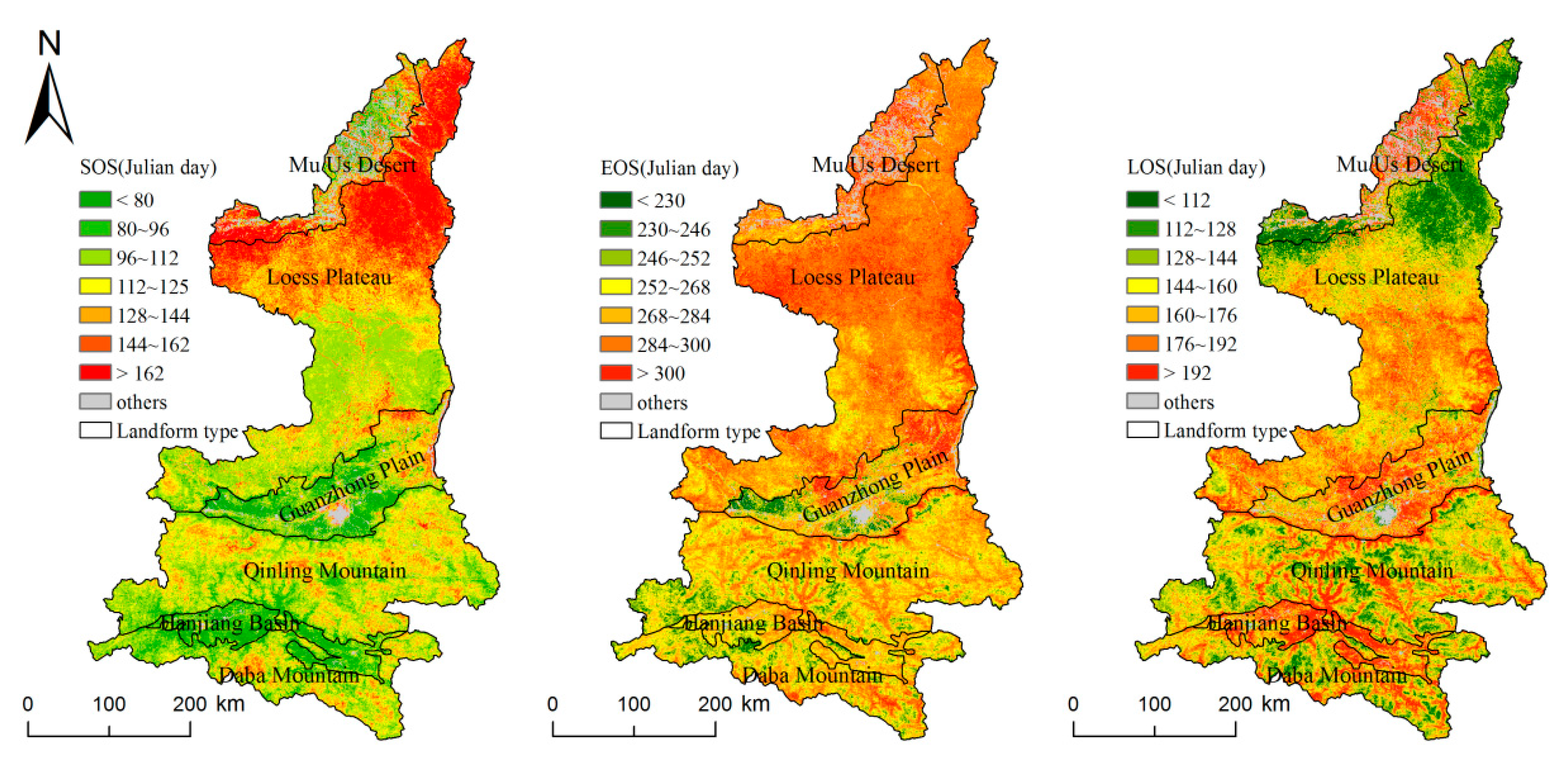
where i is the time sequence number. We determined the i value with the maximum NDVIratio and then used the corresponding Julian day as the SOS. Likewise, we determined the i value with the minimum NDVIratio and used the corresponding Julian day at i + 1 as the EOS. We extracted the phenological parameters of the vegetation in the study area pixel by pixel and saved the results as a TIF-format image in Matlab. Finally, we made a thematic map in ArcGIS, as shown in Figure 3.
2.4. Trend and Correlation Analysis
In the investigation of the temporal and spatial changes in phenology over the study area, we performed a linear regression of the phenological parameters against the SOS, EOS, and LOS and used the resulting regression coefficients to analyze the spatial-temporal trends of the phenology. The mathematical formula can be expressed as follows:
where n is the years during the monitoring period, t is a certain year, and yt is the vegetation phenological parameter value for year t. trend > 0 indicates a delayed trend, while trend < 0 indicates an advancement trend.
In order to explore the response of the phenology to the temperature, precipitation, and sunshine hours, we used Pearson’s correlation analysis. Specifically, (1) the correlations of SOS with the temperature and precipitation from February to April were evaluated; (2) the correlations between the EOS and the temperature and precipitation from September to November and the correlation between the EOS and the sunshine hours from May to July were evaluated; and (3) the correlations between the LOS and the temperature and precipitation from April to September and the correlation between the LOS and the monthly sunshine hours from May to July were evaluated. The R-value was calculated as follows:
where xt is the meteorological data for year t. yt is the phenological parameter value for year t. We performed Pearson’s correlation analysis and saved the results as a TIF-format image in Matlab, which were used to make a thematic map in ArcGIS.
3. Results
3.1. Spatial Distribution Patterns of the Multi-Annual Average Vegetation Phenology
Figure 3 shows the spatial distributions of the SOS, EOS, and LOS in different geomorphic regions of the study area during 2001–2016. As shown in the figure, the vegetation phenology throughout the study area varied with the latitude from north to south, but due to the differences in topography and climate in each geomorphic zone, the vegetation phenology exhibited spatial heterogeneity. Compared with the southern area, the northern area had a later SOS and EOS and a shorter LOS. The difference in SOS between the north and south was the most obvious, with the SOS occurring early in the south and late in the north.
Table 1 presents a statistical analysis of the spatial distribution of the vegetation phenology illustrated in Figure 3. In Shaanxi, the annual average SOS was 120 d, the annual average EOS was 280 d, and the annual average LOS was 160 d. In the northern LP, the annual average SOS was 134 d, which was greater than that in other geomorphic regions. The SOS first appeared in the HJB, where the climate is humid all year, and the altitude is relatively low, with an annual average of 88 d. The EOS was the latest in the MUD, with an annual average of 291 d, and the earliest in the DBM, at 267 d. The HJB had the longest LOS of 183 d. In the other geomorphic regions, the LOS exhibited little difference, ranging from 155 d to 173 d.
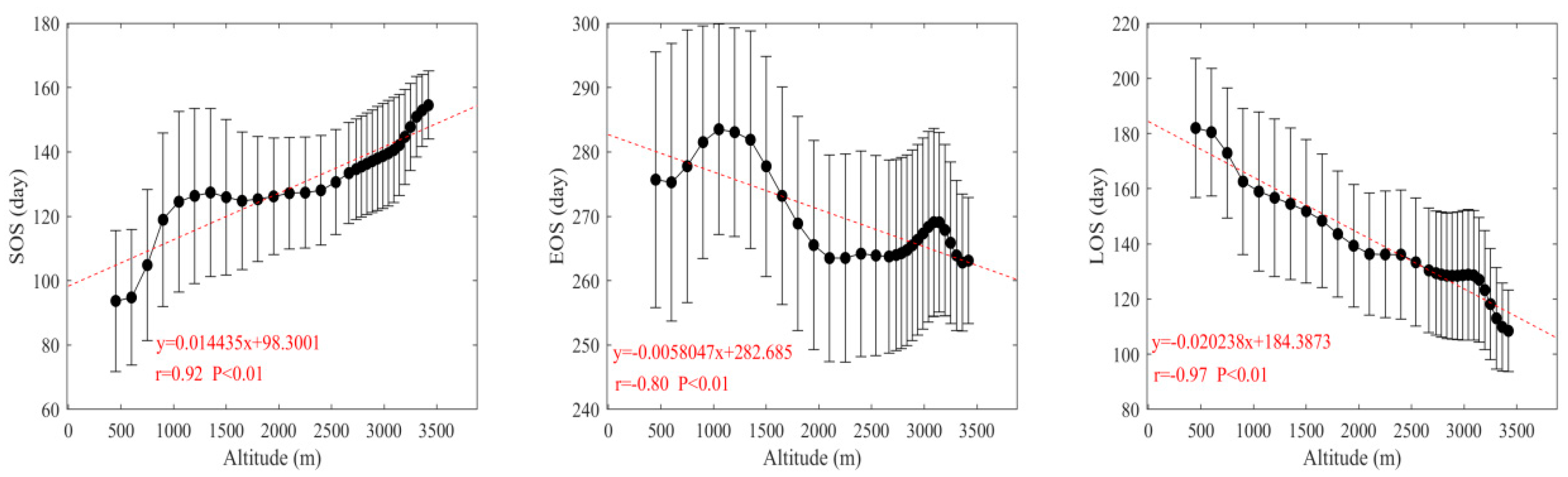
There was a close relationship between the vegetation phenology and altitude in Shaanxi. Pearson’s correlation analysis indicated that the relationship was significant. The characteristics of the changes in vegetation phenology with altitude are shown in Figure 3. The SOS was significantly delayed with increasing altitudes, and the extent of the delay was approximately 1.4 d/100 m (r = 0.92, P < 0.01). The LOS was significantly shortened at a rate of approximately 2 d/100 m (r = −0.97, P < 0.01). The EOS was both postponed and advanced with increasing altitudes, but it showed a significant advancing trend overall, with the rate of advancement of approximately 0.6 d/100 m (r = −0.80, P < 0.01).
3.2. Spatial Distribution Patterns of Interannual Phenological Changes
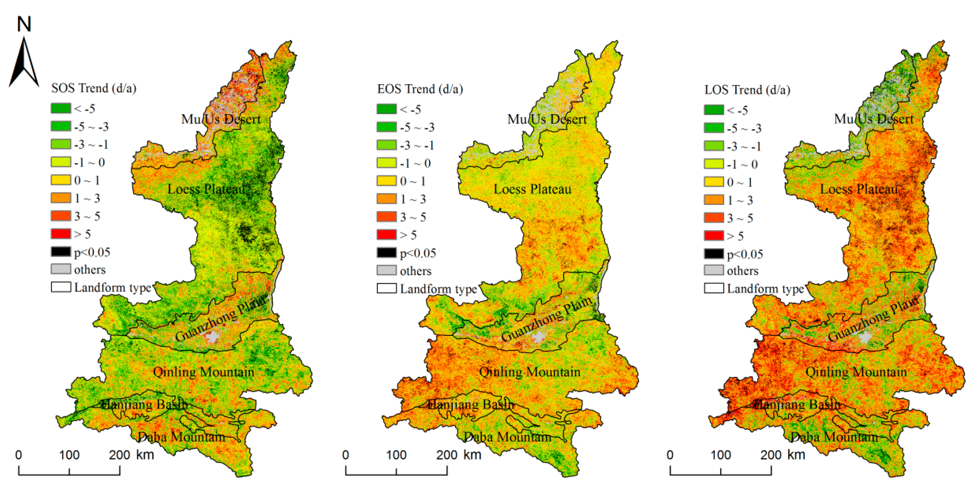
As shown as Figure 4, throughout the study area, over 66.39% of the pixels showed that the SOS had an advancing trend (0.89 d/years), and the trends of 6.89% of the pixels were significant. In the LP, the percentage of pixels with advancing trends in this area was 78.39%, and the trends were significant in 11.47% of the pixels, with a rate of advancement of 1.51 d/year. However, in the northern MUD, delayed-SOS pixels accounted for the majority, covering 71.97% of the pixels. In some geomorphic regions, the advancement of the SOS gradually weakened from north to south—for example, in the LP, the trend in the north was larger than that in the south. There were no significant differences in the EOS in terms of advancements and delays, and 53.81% of the pixels exhibited delays, while 2.48% of the pixels exhibited significant delays, with the average rate of delay of 0.18 d/year. These pixels were mainly distributed in the QLM, HJB, and LP. The highest rate of delay of 64.54% occurred in the QLM, with a rate of delay of 0.83 d/year. The areas with advancements were mainly distributed in the MUD, DBM, and GZP, with a rate of advancement of 0.34 d/year. The LOS showed an overall trend of extension, covering 65.05% of the pixels, of which 5.57% showed significant extension, with the rate of extension of 1.07 d/year, which was greater than the changes in SOS and EOS. The prolongation trends of the area were mostly in the LP and QLM, where 73.03% and 72.32% of the pixels exhibited delays. In the LP, 7.32% of the pixels exhibited significant prolongation, and the rate of prolongation in the QLM was significantly higher than the average, reaching 1.88 d/year. The shortening of the LOS was mainly concentrated in the MUD, where the shortening ratio reached 72.03% and significantly decreased to 9.76%, and the shortening time was 2.52 d/year.
3.3. The Response of the Vegetation Phenology to Climatic Factors
3.3.1. The Response of the SOS to Precipitation and Temperature
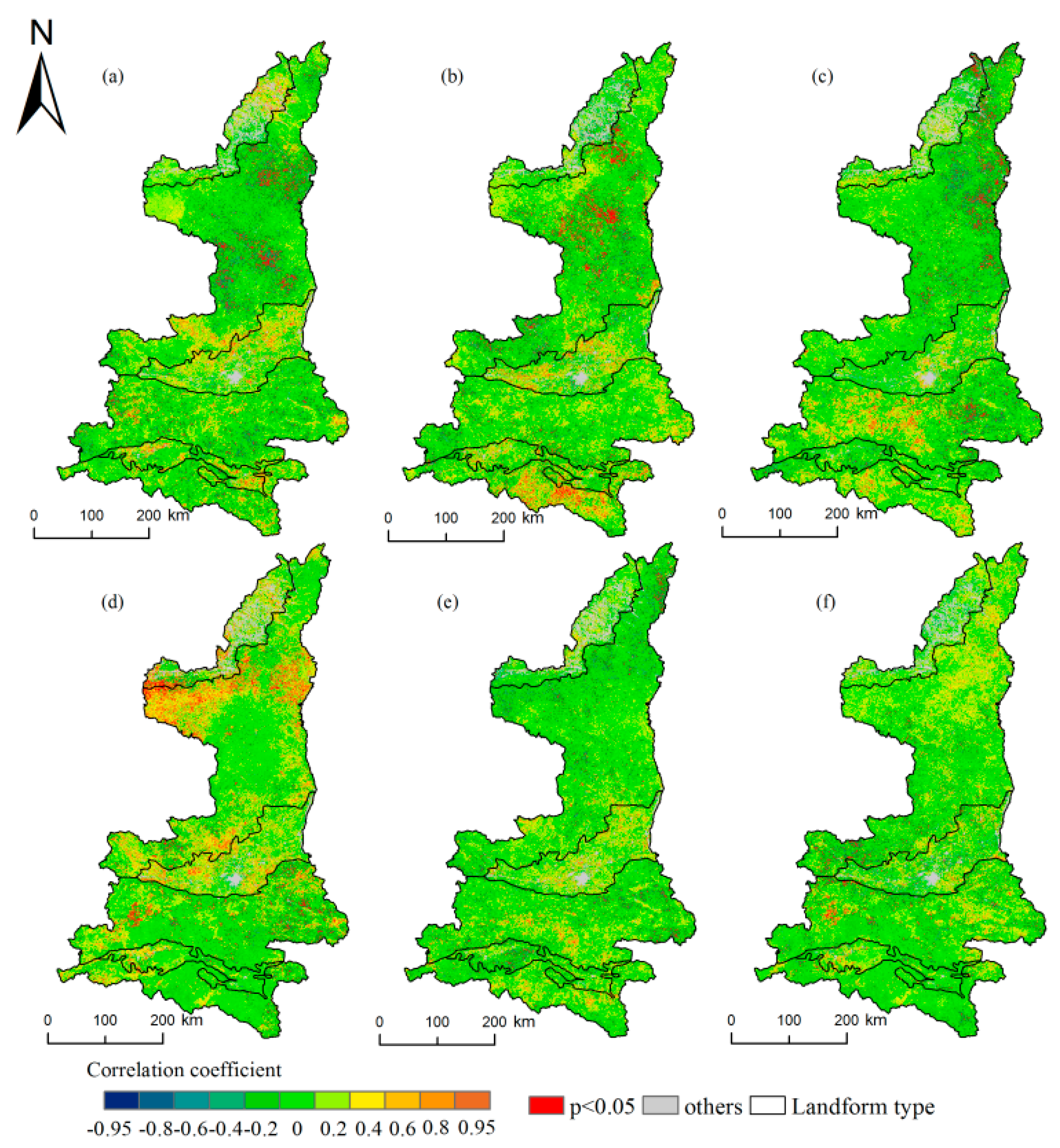
We can see from Figure 5, for the entire study area, the average precipitation from February to April had a negative correlation with the SOS, with negative correlations occurring in 61.88% of the pixels, indicating that with the increase of precipitation, the SOS advanced. The greatest influence of precipitation on the SOS occurred in March when 7.5% of the pixels exhibited significant negative correlations. The average temperature from February to April also had a negative correlation with the SOS in 58.14% of the pixels, where the SOS advanced with the increase of the temperature. However, the greatest influence of the temperature on the SOS occurred in February, with the negative correlation being significant in only 3.17% of the pixels.
The influences of the precipitation and temperature on the SOS in different geomorphic regions of the study area differed from north to south. The MUD and LP in the north were mainly affected by the temperature. In February, the temperature had the greatest influence in the MUD and LP, where the proportion of significant pixels reached 14.42% and 11.83%, respectively, which mainly exhibited positive correlations. Precipitation had a mainly negative correlation with the SOS in the MUD and LP, but fewer pixels were affected by precipitation than by the temperature. The GZP and QLM in the central region were affected by temperature and precipitation. Precipitation and temperature had mainly negative correlations in the QLM. In the GZP, precipitation and temperature had mainly positive correlations in February and March and negative correlations in April. The HJB and DBM in the south were strongly affected by precipitation. Precipitation had the greatest influence on the SOS in March in the DBM, with significant pixels accounting for 12.16% of the area, in which the correlations were positive. The delays in these regions might be due to the increase in precipitation, which might have resulted in a decrease in the temperature and a delay of the SOS. However, the response to temperature was weak in the DBM, and the largest proportion of significant pixels in March was only 2.74%, which was far less than those in other areas.
3.3.2. The Response of the EOS to Precipitation, Temperature, and Sunshine Hours
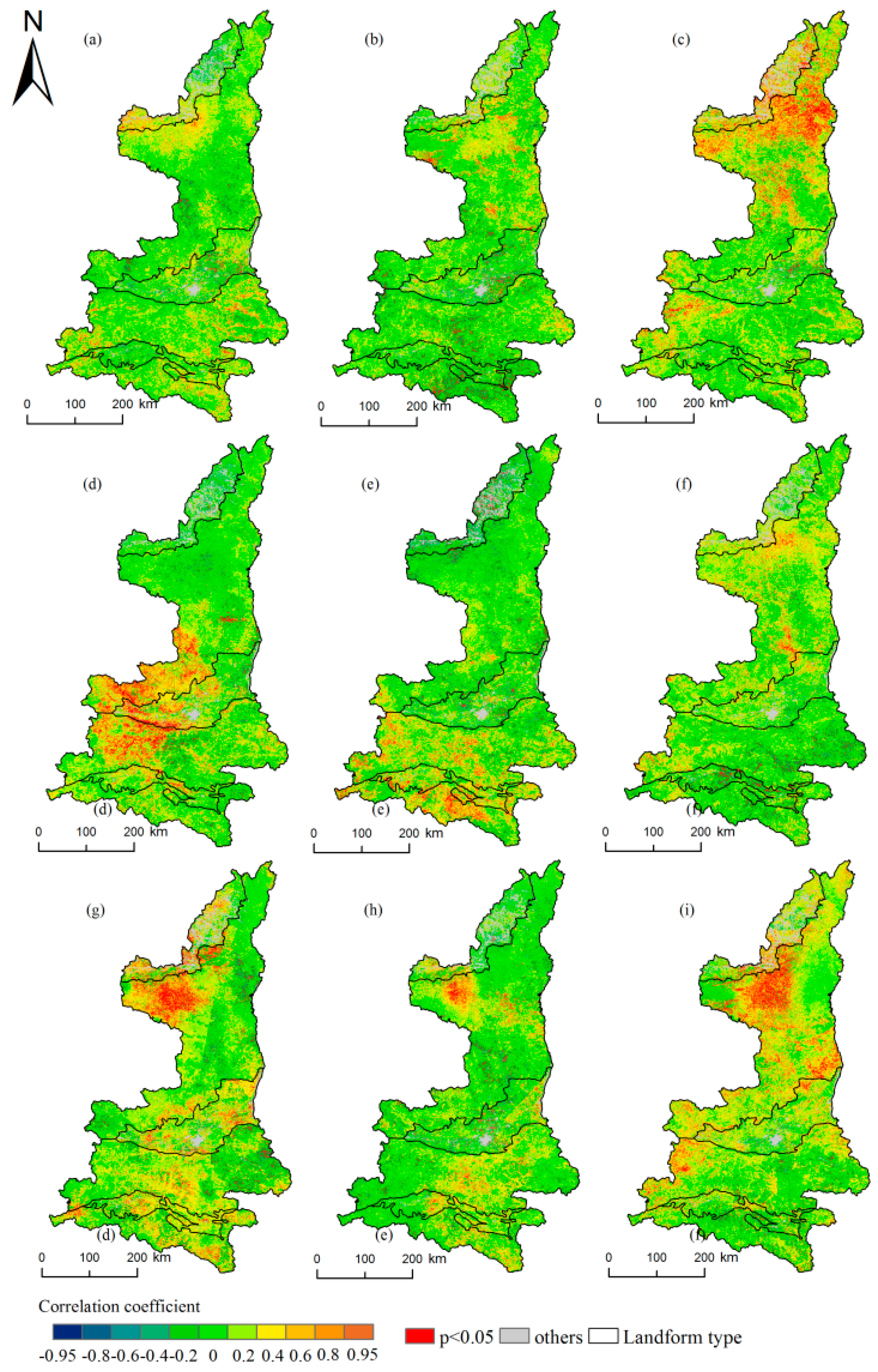
As shown as Figure 6, compared with the SOS, the impacts of the Spatio-temporal variations in the climate on the EOS were more complex. There were limited positive and negative correlations between the EOS and precipitation in September and October, and there were few significant pixels. Precipitation had the greatest influence on the EOS in November. positive correlations covered 64.88% of the area, and the influence was significant in 10.73% of the pixels, indicating that the EOS was delayed in most regions with the increase of precipitation. There were limited positive and negative correlations between the EOS and temperature from September to November. The greatest influence of the temperature on the EOS occurred in September, and 10.13% of the pixels exhibited significant positive correlations. The influence of the sunshine hours on the EOS was positive from May to July. This result indicated that the EOS was delayed as the sunshine hours increased. In May and July, there were no significant differences in the effects of the sunshine hours on the EOS, and the influences were significant in 8.75% and 9.63% of the pixels, respectively, compared with 4.58% in June.
Similar to the SOS, the response of the EOS to the climate also showed differences between the north and south. However, in contrast to the SOS, the temperature had a mainly positive correlation in the central and southern areas of the study area to the south of the GZP. The temperature in September had the greatest influence in the GZP and QLM, at 15.97%, while 12.61% of the pixels exhibited significant positive correlations. In contrast, in the DBM and HJB, the temperature had the greatest influence in October, when the proportions of pixels with significant positive correlations reached 12.97% and 10.82%, respectively. Precipitation mainly affected the MUD and LP in the north of the study area. The greatest impact from precipitation on the EOS in the MUD and LP occurred in November, when significant positive correlations occurred in 17.85% and 16.11% of the pixels, respectively. This finding indicated that the EOS was delayed with the increase of precipitation. In summer, most of the plants are luxuriant. The sunshine hours affect changes in the EOS and LOS by affecting photosynthesis [52]. The greatest effects of the sunshine hours on the EOS occurred in the MUD and LP, and the correlations were mainly positive. This finding indicated that the EOS was delayed as the sunshine intensified. The highest proportion of significant pixels was 16.61%, which occurred in the MUD in May, while 13.61% were significant in the LP in July. In other areas, the effects of the sunshine hours on the EOS were mainly positive, but the number of significant pixels was low.
3.3.3. The Response of the LOS to the Precipitation, Temperature, and Sunshine
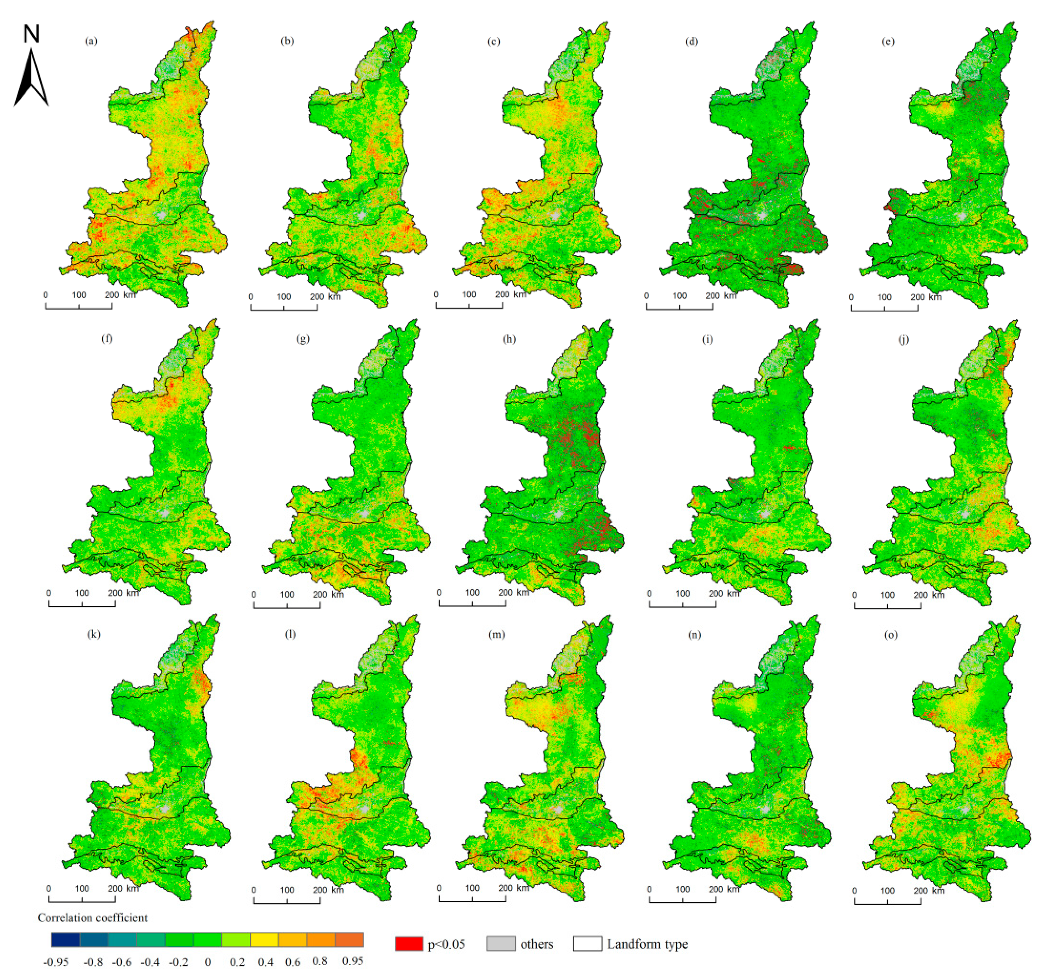
Figure 7 shows the direction of the correlation coefficient between the precipitation and LOS changed from April to September. Positive correlations covered 70.12% of the area from April to June, and negative correlations covered 74.18% of the area in July and August. In September, about 57.6% of the area showed a positive correlation between the LOS and precipitation. The greatest influence of precipitation on the LOS reached 12.62% in July, which was a significant negative correlation. This result showed that the LOS in most areas would be shortened with the increase of precipitation in July. The proportions of positive and negative correlations of the LOS with the temperature from April to September were 45.03% and 54.97%, respectively. The greatest influence of the temperature on the LOS reached 72.41% in May when the correlation was negative, whereas 12.03% of the pixels exhibited positive correlations. The influence of the sunshine hours on the LOS was less significant than the influences of precipitation and temperature. The effect of the sunshine hours on the LOS was the most significant in May when the proportion of significant pixels was 6.85%. There were positive correlations in May and July and negative correlations in June.
In contrast to the SOS and EOS, the influence of the climate on the LOS exhibited Spatio-temporal heterogeneity and no regularity. Precipitation had the greatest effect on the LOS in most regions in July, and the correlations were mainly negative. The largest correlation occurred in the HJB, where 17.41% of the pixels showed significant correlations. In the LP, the greatest effects of precipitation on the LOS occurred in August, when 10.19% of the pixels showed significant correlations. In April, the temperature had the greatest effect in the DBM, and the significant pixel ratio was 8.55%, with most being positively correlated. In May, the temperature had the greatest effect in the LP and QLM, and the proportions of significant pixels were 13.66% and 14.23%, respectively, which mainly exhibited negative correlations. The GZP was most affected by the temperature in September when the proportion of significant pixels was 8.98%. The LOS in the MUD was not affected by the temperature, and the average ratio of significant pixels was only 2.29%, which was much lower than those in other areas. The influence of the sunshine hours on each geomorphic area was positive, and the greatest effect was observed in May. The highest proportion of significant pixels was 9.93% in the DBM. The influence of the sunshine hours in the other regions was not significantly different, and the proportion of significant pixels was less than 6% from May to July.
4. Discussion
The extent to which climatic factors influence the vegetation phenology is dependent on the different developmental stages of the phenological events [5]. Moreover, the responses of the vegetation phenology to environmental changes are non-uniform in different regions [52], in which the climate and vegetation type can differ greatly. Under normal conditions, the northern arid area experiences less precipitation and lower temperatures than does the south in autumn, so the EOS should be earlier. However, interestingly, the EOS in the northern area was found to be significantly later than that in the southern area in our study. This difference might arise because the vegetation in the north is mostly Artemisia and herbaceous plants, for which the EOS occurs around the end of October or the middle of November, which is later than the EOS for corn, wheat, and other crops in the south. This finding showed that the responses of the EOS to climate changes were more complex than those of the SOS, and the two trends are asymmetric [3,11].
Vegetation phenology was influenced by human activities. Interannual variations in the phenology indicated that the SOS was undergoing an advancement trend, while the LOS was being prolonged. However, in the two adjacent climatic regions in the north, the results were the opposite. In the LP, the SOS underwent the most significant advancement, while the LOS was extended. For the MUD, the SOS was delayed, and the LOS was shortened. This trend occurred mainly because the main vegetation comprises shrubs and grassland in the LP, which are more sensitive to temperature changes than the other types of vegetation. Because trees have been planted to control desertification in the MUD over the past decade, the ecological environment has improved, and the vegetation coverage has increased from 9.9% in 2000 to 38.03% in 2018 (http://www.shaanxi.gov.cn). The vegetation type also changed from Salix and other wind-break plants to crops, such as potatoes and corn (sprouting in May and harvested in October), which have a later SOS and a shorter LOS than those of forest and grass plants.
Most studies have found temperature to be the main factor that controls the vegetation phenology [53,54]. In this study, precipitation was shown to play a role as critical as that of the temperature. For the SOS, most areas of the MUD and LP were mainly affected by the temperature in the north. The central GZP and QLM were affected by both the temperature and precipitation, and the precipitation in the HJB and DBM was the key factor in the south. However, for the EOS, precipitation mainly affected most of the northern region, while the central and southern regions were mainly affected by the temperature. These results showed that the effects of climate changes on the vegetation phenology were complex. These impacts differed by region, and the climate factors that control the vegetation phenology were different in different geomorphic areas. Similarly, we found that the sunshine hours were positively correlated with the EOS from May to July. This finding was consistent with the results of previous studies [55]. When summer transitions into autumn, the day gradually shortens (the sunshine hours decrease), which induces bud setting and leaf senescence [56].
Vegetation phenology was affected by different climate factors. In the northern MUD, the SOS was most significantly affected by the temperature. In contrast, in the southern DBM, precipitation had the largest influence on the SOS, whereas the temperature had the least influence. This phenomenon might be due to the lower temperature in spring in the north, and the increase of the temperature was key to breaking the dormancy of plants. For the warm south, the effect of precipitation was more important than that of temperature for the growth of plants. Furthermore, in different geomorphic areas, the response relationships and correlation coefficients were different between the vegetation phenology and climate changes. In February, the temperatures in the LP and MUD were positively correlated with the SOS, while in the HJB and DBM, they were negatively correlated. The precipitation in October was negatively correlated with the EOS in the QLM, HJB, DBM, and GZP, while in the LP and MUD, they were positively correlated in November. In some northern arid areas, the increase of the temperature in spring might lead to the decrease of the soil moisture and have a negative impact on plant growth, while in southern humid areas, the increase of precipitation in autumn would lead to the decrease of the temperature, and plant growth would stop early.
5. Conclusions
In the context of global warming, quantifying the responses of phenology to climate drivers is essential for the sustainable development of ecosystems. This study analyzed the spatial differentiation of the phenology and the spatial-temporal variation of the phenology in six different geomorphological landscapes in Shaanxi, China, and discussed the responses of the phenology to climate changes. The main conclusions are as follows:
- (1)
- The phenology varied with latitude. The SOS in the south was earlier, whereas that in the north was later.
- (2)
- In the whole region, the SOS was gradually being advanced, while the LOS was being prolonged, but in the MUD, the SOS was being delayed, and the LOS was being shortened. The variation in the phenology had spatial heterogeneity among different geomorphological areas.
- (3)
- The responses of the phenology to climatic factors were very complex. In the north, the SOS was mainly affected by the temperature in February, and the EOS was mainly affected by the precipitation in November. In the south, the SOS was mainly affected by the precipitation in March, and the EOS was affected by the temperature in October.
Our results showed that the phenology was very sensitive to the climate, and there might be different types of phenology due to different topography and vegetation types. These findings might help reveal local phenological patterns related to microclimates and in understanding phenology at different scales.
Author Contributions
Conceptualization, Jianjun Bai and Hongzhu Han; methodology, Hongzhu Han; formal analysis, Hongzhu Han and Gao Ma; investigation, Gao Ma; writing—original draft preparation, Hongzhu Han; writing—review and editing, Jianjun Bai and Jianwu Yan; funding acquisition, Jianjun Bai and Jianwu Yan. All authors have read and agreed to the published version of the manuscript
Funding
This research was funded by the National Natural Science Foundation of China, grant number [41171310 and 41501093] and the Natural Science Basic Research Program of Shaanxi, grant number [2016JM4016].
Acknowledgments
The authors would like to thank all the reviewers for their invaluable comments and suggestions for this manuscript.
Conflicts of Interest
The authors declare no conflict of interest.
References
- Miller-Rushing, A.J.; Weltzin, J. Phenology as a tool to link ecology and sustainable decision making in a dynamic environment. New Phytol. 2009, 184, 743–745. [Google Scholar] [CrossRef] [PubMed]
- Helmut, L.P.D. Phenology and Seasonality Modeling. Ecol. Stud. 1974, 120, 461. [Google Scholar]
- Jeong, S.J.; Chang-Hoi, H.O.; Gim, H.J.; Brown, M.E. Phenology shifts at start vs. end of growing season in temperate vegetation over the Northern Hemisphere for the period 1982–2008. Glob. Chang. Boil. 2011, 17, 2385–2399. [Google Scholar] [CrossRef]
- Zheng, J.; Ge, Q.; Hao, Z. Impacts of climate warming on plants phenophases in China for the last 40 years. Chin. Sci. Bull. 2002, 47. [Google Scholar]
- Piao, S.L.; Liu, Q.; Chen, A.P.; Janssens, I.A.; Fu, Y.S.; Dai, J.H.; Liu, L.L.; Lian, X.; Shen, M.G.; Zhu, X.L. Plant phenology and global climate change: Current progresses and challenges. Glob. Chang. Boil. 2019, 25, 1922–1940. [Google Scholar] [CrossRef]
- Keeling, C.D.; Chin, J.F.S.; Whorf, T.P. Increased activity of northern vegetation inferred from atmospheric CO2 measurements. Nature 1996, 382, 146–149. [Google Scholar] [CrossRef]
- Pe?Uelas, J.; Filella, I. Phenology. Responses to a warming world. Science 2001, 294, 793–795. [Google Scholar] [CrossRef]
- Wang, X.; Xiao, J.; Li, X.; Cheng, G.; Ma, M.; Zhu, G.; Arain, M.A.; Black, T.A.; Jassal, R.S. No trends in spring and autumn phenology during the global warming hiatus. Nat. Commun. 2019, 10, 2389. [Google Scholar] [CrossRef]
- Williams, S.E.; Bolitho, E.E.; Fox, S. Climate change in Australian tropical rainforests: An impending environmental catastrophe. Proc. Boil. Sci. 2003, 270, 1887–1892. [Google Scholar] [CrossRef]
- Lee, S.-D. Global Warming Leading to Phenological Responses in the Process of Urbanization, South Korea. Sustainability 2017, 9, 2203. [Google Scholar] [CrossRef] [Green Version]
- Richardson, A.D.; Keenan, T.F.; Migliavacca, M.; Ryu, Y.; Sonnentag, O.; Toomey, M. Climate change, phenology, and phenological control of vegetation feedbacks to the climate system. Agric. For. Meteorol. 2013, 169, 156–173. [Google Scholar] [CrossRef]
- Badeck, F.W.; Bondeau, A.K.; Doktor, D.; Lucht, W.; Schaber, J. Responses of spring phenology to climate change [Review]. New Phytol. 2004, 162, 295–309. [Google Scholar] [CrossRef]
- Schwartz, M.D. Green-wave phenology. Nature 1998, 394, 839–840. [Google Scholar] [CrossRef]
- Bradley, N.L.; Leopold, A.C.; Ross, J.; Huffaker, W. Phenological changes reflect climate change in Wisconsin. Proc. Natl. Acad. Sci. USA 1999, 96, 9701–9704. [Google Scholar] [CrossRef] [Green Version]
- Menzel, A.; Fabian, P. Growing season extended in Europe. Nature 1999, 397, 659. [Google Scholar] [CrossRef]
- Saxe, H.; Johnsen, Ø.; Ryan, M.G.; Vourlitis, G. Tansley Review No. 123. Tree and Forest Functioning in Response to Global Warming. New Phytol. 2010, 149, 369–399. [Google Scholar] [CrossRef]
- Linkosalo, T.; Häkkinen, R.; Terhivuo, J.; Tuomenvirta, H.; Hari, P. The time series of flowering and leaf bud burst of boreal trees (1846–2005) support the direct temperature observations of climatic warming. Agric. For. Meteorol. 2009, 149, 453–461. [Google Scholar] [CrossRef]
- Delbart, N.; Picard, G.; Toan, T.L.; Kergoat, L.; Quegan, S.; Woodward, I.; Dye, D.; Fedotova, V. Spring phenology in boreal Eurasia over a nearly century time scale. Glob. Chang. Boil. 2010, 14, 603–614. [Google Scholar] [CrossRef]
- Nordli, O.; Wielgolaski, F.E.; Bakken, A.K.; Hjeltnes, S.H.; Mage, F.; Sivle, A.; Skre, O. Regional trends for bud burst and flowering of woody plants in Norway as related to climate change. Int. J. Biometeorol. 2008, 52, 625–639. [Google Scholar] [CrossRef]
- Pudas, E.; Leppälä, M.; Tolvanen, A.; Poikolainen, J.; Venäläinen, A.; Kubin, E. Trends in phenology of Betula pubescens across the boreal zone in Finland. Int. J. Biometeorol. 2008, 52, 251–259. [Google Scholar] [CrossRef]
- Menzel, A.; Sparks, T.H.; Estrella, N.; Koch, E.; Aasa, A.; Ahas, R.; Alm-Kübler, K.; Bissolli, P.; Braslavská, O.; Briede, A.; et al. European phenological response to climate change matches the warming pattern. Glob. Chang. Boil. 2006, 12, 1969–1976. [Google Scholar] [CrossRef]
- Fu, Y.H.; Shilong, P.; Hongfang, Z.; Su-Jong, J.; Xuhui, W.; Yann, V.; Philippe, C.; Janssens, I.A. Unexpected role of winter precipitation in determining heat requirement for spring vegetation green-up at northern middle and high latitudes. Glob. Chang. Biol. 2015, 20, 3743–3755. [Google Scholar] [CrossRef] [PubMed]
- Vitasse, Y.; Delzon, S.; Dufrêne, E.; Pontailler, J.Y.; Louvet, J.M.; Kremer, A.; Michalet, R. Leaf phenology sensitivity to temperature in European trees: Do within-species populations exhibit similar responses? Agric. For. Meteorol. 2009, 149, 735–744. [Google Scholar] [CrossRef]
- Miller-Rushing, A.J.; Primack, R.B. Global warming and flowering times in Thoreau’s Concord: a community perspective. Ecology 2008, 89, 332–341. [Google Scholar] [CrossRef]
- Sparks, T.; Carey, P.D.; Combes, J. First leafing dates of trees in Surrey between 1947 and 1996. Lond. Nat. 1997, 76, 15–20. [Google Scholar]
- Cong, N.; Wang, T.; Nan, H.; Ma, Y.; Wang, X.; Myneni, R.B.; Piao, S. Changes in satellite-derived spring vegetation green-up date and its linkage to climate in China from 1982 to 2010: a multimethod analysis. Glob. Chang. Boil. 2013, 19, 881–891. [Google Scholar]
- Solomon, S.; Qin, D.; Manning, M.; Chen, Z.; Marquis, M.; Averyt, K.B.; Tignor, M.; Miller, H.L.; Solomon, S.; Qin, D. Climate change 2007: the Physical Science Basis. Contribution of Working Group I to the Fourth Assessment Report of the Intergovernmental Panel on Climate Change. Summary for Policymakers. Intergov. Panel Clim. Chang. Clim. Chang. 2007, 18, 95–123. [Google Scholar]
- Yun, J.; Jeong, S.J.; Ho, C.H.; Park, C.E.; Kim, J. Influence of winter precipitation on spring phenology in boreal forests. Glob. Chang. Boil. 2018, 24, 5176–5187. [Google Scholar] [CrossRef]
- Fu, Y.H.; Piao, S.; Vitasse, Y.; Zhao, H.; De Boeck, H.J.; Liu, Q.; Yang, H.; Weber, U.; Janssens, I.A. Increased heat requirement for leaf flushing in temperate woody species over 1980-2012: effects of chilling, precipitation and insolation. Glob. Chang. Biol. 2015, 21, 2687–2697. [Google Scholar] [CrossRef]
- Jin, H.; Jonsson, A.M.; Olsson, C.; Lindstrom, J.; Jonsson, P.; Eklundh, L. New satellite-based estimates show significant trends in spring phenology and complex sensitivities to temperature and precipitation at northern European latitudes. Int. J. Biometeorol. 2019, 63, 763–775. [Google Scholar] [CrossRef] [Green Version]
- Wright, S.J.; Schaik, C.P.V. Light and the Phenology of Tropical Trees. Am. Nat. 1994, 143, 192–199. [Google Scholar] [CrossRef]
- Zimmerman, J.K.; Wright, S.J. Flowering and Fruiting Phenologies of Seasonal and Aseasonal Neotropical Forests: The Role of Annual Changes in Irradiance. J. Trop. Ecol. 2007, 23, 231–251. [Google Scholar] [CrossRef] [Green Version]
- Reich, P.B. Phenology of tropical forests: patterns, causes, and consequences. Can. J. Bot. 1995, 73, 164–174. [Google Scholar] [CrossRef]
- Morisette, J.T.; Richardson, A.D.; Knapp, A.K.; Fisher, J.I.; Graham, E.A.; Abatzoglou, J.; Wilson, B.E.; Breshears, D.D.; Henebry, G.M.; Hanes, J.M.; et al. Tracking the rhythm of the seasons in the face of global change: phenological research in the 21st century. Front. Ecol. Environ. 2009, 7, 253–260. [Google Scholar] [CrossRef] [Green Version]
- Ge, Q.; Dai, J.; Zheng, J. The Progress of Phenology Studies and Challenges to Modern Phenology Research in China. Bull. Chin. Acad. Sci. 2010, 25, 310–316. [Google Scholar] [CrossRef]
- Piao, S.; Fang, J.; Zhou, L.; Ciais, P.; Zhu, B. Variations in satellite-derived phenology in China’s temperate vegetation. Glob. Chang. Boil. 2006, 12, 672–685. [Google Scholar] [CrossRef]
- Liu, L.L.; Liang, L.; Schwartz, M.D.; Donnelly, A.; Wang, Z.; Schaaf, C.B.; Liu, L.Y. Evaluating the potential of MODIS satellite data to track temporal dynamics of autumn phenology in a temperate mixed forest. Remote Sens. Environ. 2015, 160, 156–165. [Google Scholar] [CrossRef]
- Li, H.; Wang, C.; Zhang, L.; Li, X.; Zang, S. Satellite monitoring of boreal forest phenology and its climatic responses in Eurasia. Int. J. Remote Sens. 2017, 38, 5446–5463. [Google Scholar] [CrossRef]
- Yuan, M.; Wang, L.; Lin, A.; Liu, Z.; Qu, S. Variations in land surface phenology and their response to climate change in Yangtze River basin during 1982-2015. Theor. Appl. Clim. 2019, 137, 1659–1674. [Google Scholar] [CrossRef]
- Ren, S.; Yi, S.; Peichl, M.; Wang, X. Diverse Responses of Vegetation Phenology to Climate Change in Different Grasslands in Inner Mongolia during 2000-2016. Remote Sens. 2018, 10, 17. [Google Scholar] [CrossRef] [Green Version]
- Zhu, W.; Zheng, Z.; Jiang, N.; Zhang, D. A comparative analysis of the spatio-temporal variation in the phenologies of two herbaceous species and associated climatic driving factors on the Tibetan Plateau. Agric. For. Meteorol. 2018, 248, 177–184. [Google Scholar] [CrossRef]
- Cheng, M.; Jin, J.; Zhang, J.; Jiang, H.; Wang, R. Effect of climate change on vegetation phenology of different land-cover types on the Tibetan Plateau. Int. J. Remote Sens. 2018, 39, 470–487. [Google Scholar] [CrossRef]
- Williams, J.W.; Jackson, S.T.; Kutzbach, J.E. Projected distributions of novel and disappearing climates by 2100 AD. Proc. Natl. Acad. Sci. USA 2007, 104, 5738–5742. [Google Scholar] [CrossRef] [PubMed] [Green Version]
- Shaowei, Z.; Yong, G.; Honghua, Q. Fundamental Relief Types and Their Classification Index Used in Provincial Geographic Conditions Monitoring in Shaanxi. Stand. Surv. Mapp. 2012, 28, 13–16. [Google Scholar]
- Song, C.-Q.; Ke, L.-H.; You, S.-C.; Liu, G.-H.; Zhong, X.-K. Comparison of Three NDVI Time-series Fitting Methods based on TIMESAT—Taking the Grassland in Northern Tibet as Case. Remote Sens. Technol. Appl. 2011, 26, 147–155. [Google Scholar]
- Goward, S.N.; Markham, B.; Dye, D.G.; Dulaney, W.; Yang, J. Normalized difference vegetation index measurements from the advanced very high resolution radiometer. Remote Sens. Environ. 1992, 35, 257–277. [Google Scholar] [CrossRef]
- Chen, J.; Jönsson, P.; Tamura, M.; Gu, Z.; Matsushita, B.; Eklundh, L. A simple method for reconstructing a high-quality NDVI time-series data set based on the Savitzky–Golay filter. Remote Sens. Environ. 2004, 91, 332–344. [Google Scholar] [CrossRef]
- Zhang, X.; Friedl, M.A.; Schaaf, C.B.; Strahler, A.H.; Hodges, J.C.F.; Gao, F.; Reed, B.C.; Huete, A. Monitoring vegetation phenology using MODIS. Remote Sens. Environ. 2003, 84, 471–475. [Google Scholar] [CrossRef]
- Zhou, L.; Tucker, C.J.; Kaufmann, R.K.; Slayback, D.; Myneni, R.B. Variation in northern vegetation activity inferred from satellite data of vegetation index during 1981 to 1999. J. Geophys. Res. Atmos. 2001, 106, 20069–20084. [Google Scholar] [CrossRef]
- Haiying, Y.; Eike, L.; Jianchu, X. Winter and spring warming result in delayed spring phenology on the Tibetan Plateau. Proc. Natl. Acad. Sci. USA 2010, 107, 22151–22156. [Google Scholar]
- Kafaki, S.B.; Mataji, A.; Hashemi, S.A. Monitoring growing season length of deciduous broad leaf forest derived from satellite data in Iran. Am. J. Environ. Sci. 2009, 5, 647–652. [Google Scholar] [CrossRef] [Green Version]
- Keenan, T.F. Phenology: Spring greening in a warming world. Nature 2015, 526, 48–49. [Google Scholar] [CrossRef] [PubMed] [Green Version]
- Richardson, A.D.; Anderson, R.S.; Arain, M.A.; Barr, A.G.; Bohrer, G.; Chen, G.; Chen, J.M.; Ciais, P.; Davis, K.J.; Desai, A.R. Terrestrial biosphere models need better representation of vegetation phenology: Results from the North American Carbon Program Site Synthesis. Glob. Chang. Boil. 2012, 18, 566–584. [Google Scholar] [CrossRef] [Green Version]
- Wolkovich, E.M.; Cook, B.I.; Allen, J.M.; Crimmins, T.M.; Betancourt, J.L.; Travers, S.E.; Pau, S.; Regetz, J.; Davies, T.J.; Kraft, N.J.B.; et al. Warming experiments underpredict plant phenological responses to climate change. Nature 2012, 485, 494–497. [Google Scholar] [CrossRef]
- Cooke, J.E.K.E.; Maria, E.; Junttila, O. The dynamic nature of bud dormancy in trees: environmental control and molecular mechanisms. Plant Cell Environ. 2012, 35, 1707–1728. [Google Scholar] [CrossRef]
- Wareing, P.F. Photoperiodism in Woody Plants. Annu. Rev. Plant Physiol. 1956, 7, 191–214. [Google Scholar] [CrossRef]
Figure 1.
Study area.

Figure 2.
The normalized difference vegetation index (NDVI) time series curves of a certain pixel in 2001 in the study area.
Figure 2.
The normalized difference vegetation index (NDVI) time series curves of a certain pixel in 2001 in the study area.

Figure 3.
Spatial distribution of the multi-annual mean vegetation phenology in Shaanxi and its relationship with the altitude from 2001 to 2016.
Figure 3.
Spatial distribution of the multi-annual mean vegetation phenology in Shaanxi and its relationship with the altitude from 2001 to 2016.


Figure 4.
Spatial distribution of the inter-annual variation of the vegetation phenology in Shaanxi from 2001 to 2016 (d/a: day per year).
Figure 4.
Spatial distribution of the inter-annual variation of the vegetation phenology in Shaanxi from 2001 to 2016 (d/a: day per year).

Figure 5.
Spatial distribution of the correlation coefficients between the start of the growing season (SOS) and precipitation/temperature. (a–c) indicate the precipitation from February to April; (d–f) indicate the temperature from February to April.
Figure 5.
Spatial distribution of the correlation coefficients between the start of the growing season (SOS) and precipitation/temperature. (a–c) indicate the precipitation from February to April; (d–f) indicate the temperature from February to April.

Figure 6.
Spatial distribution of the correlation coefficients between the end of the growing season (EOS) and precipitation/temperature/sunshine and their histograms in Shaanxi. (a–c) indicate the precipitation from September to November; (d–f) indicate the temperature from September to November, respectively; (g–i) indicate the sunshine from May to July.

Figure 7.
Spatial distribution of the correlation coefficients between the LOS and precipitation/temperature/sunshine and their histograms in Shaanxi. (a–f) indicate the precipitation from April to September; (g–l) indicate the temperature from April to September; (m–o) indicate the sunshine from May to July.


Table 1.
Multi-annual mean vegetation phenology in different regions (day).
| SOS | EOS | LOS | ||||
|---|---|---|---|---|---|---|
| mean | std | mean | std | mean | std | |
| Shaanxi | 120.68 | 28.36 | 280.04 | 18.47 | 160.36 | 29.33 |
| Mu Us Desert | 132.58 | 36.80 | 291.07 | 12.59 | 158.49 | 46.64 |
| Loess Plateau | 134.16 | 27.72 | 289.65 | 11.97 | 155.50 | 28.21 |
| Guanzhong Plain | 101.02 | 27.31 | 274.90 | 25.70 | 173.88 | 26.66 |
| Qinling Mountain | 113.43 | 16.87 | 270.24 | 16.27 | 156.81 | 25.48 |
| Hanjiang Basin | 88.10 | 15.21 | 271.81 | 15.29 | 183.72 | 23.14 |
| Daba Mountain | 109.51 | 17.96 | 267.08 | 17.13 | 157.57 | 25.42 |
SOS: start of the growing season; EOS: end of the growing season; LOS: length of the growing season.
© 2020 by the authors. Licensee MDPI, Basel, Switzerland. This article is an open access article distributed under the terms and conditions of the Creative Commons Attribution (CC BY) license (http://creativecommons.org/licenses/by/4.0/).
Share and Cite
MDPI and ACS Style
Han, H.; Bai, J.; Ma, G.; Yan, J. Vegetation Phenological Changes in Multiple Landforms and Responses to Climate Change. ISPRS Int. J. Geo-Inf. 2020, 9, 111. https://0-doi-org.brum.beds.ac.uk/10.3390/ijgi9020111
AMA Style
Han H, Bai J, Ma G, Yan J. Vegetation Phenological Changes in Multiple Landforms and Responses to Climate Change. ISPRS International Journal of Geo-Information. 2020; 9(2):111. https://0-doi-org.brum.beds.ac.uk/10.3390/ijgi9020111
Chicago/Turabian StyleHan, Hongzhu, Jianjun Bai, Gao Ma, and Jianwu Yan. 2020. "Vegetation Phenological Changes in Multiple Landforms and Responses to Climate Change" ISPRS International Journal of Geo-Information 9, no. 2: 111. https://0-doi-org.brum.beds.ac.uk/10.3390/ijgi9020111
Note that from the first issue of 2016, this journal uses article numbers instead of page numbers. See further details here.