Smart Tour Route Planning Algorithm Based on Naïve Bayes Interest Data Mining Machine Learning

Abstract

A smart tour route planning algorithm based on a Naïve Bayes interest data mining machine learning is brought forward in the paper, according to the problems of current tour route planning methods. A machine learning model of Naïve Bayes interest data mining is set up by learning a mass of training data on tourists’ interests and needs. Through the recommended interest tourist site classifications from the machine learning module, the optimal tourist site mining algorithm based on the membership degree searching propagating tree of a tourist’s temporary accommodation is set up, which mines and outputs the optimal tourist sites. The mined optimal tourist sites are taken as seed points to set up a tour route planning algorithm based on the optimal propagating tree of a closed-loop structure. Through the proposed algorithm, an experiment is designed and performed to output optimal tour routes conforming to tourists’ needs and interests, including the propagating tree closed-loop structures, a minimum heap of propagating tree weight function value, and a weight function value complete binary tree. We prove that the proposed algorithm has the features of intelligence and accuracy, and it can learn tourists’ needs and interests to output optimal tourist sites and tour routes and ensure that tourists can get the best motive benefits and travel experience in the tour process, by analyzing the experiment data and results.

1. Introduction

Tour route planning is an important and indispensable content for smart tourism research and tourism geographic information system (GIS) development. Tourists are the most critical component of tourism activities, and they play a vital part in the considerable development and progress of smart tourism and tourism economies. The satisfaction degree of the motive benefits obtained in the whole tour process will directly influence a tourist’s subjective evaluations on a certain tourism city, as well as its tourist sites and tourism facilities and, thus, indirectly influence the subsequent tourists when making their travel schedule. Before visiting an unfamiliar city, tourists will initially make proper travel schedule according to their interests, time, cost budget, etc., in which the tour route is dispensable. A superior tour route will help tourists find the best motive benefits and travel experience [1,2,3].

In the development process of smart tourism and tourism GIS, embedding smart tour route planning and recommending function is an important way for tourism recommendation system to realize intelligence, the core technique is in the designing and developing of smart tour route planning algorithms. Traditional tour route planning depends on two methods, one is tourists making schedules by themselves, the other is tourists purchasing tour routes provided by a travel agency [4,5,6]. For the first method, under the condition of tourists’ being unfamiliar with the tourism city, they usually receive tourism information from websites, books, magazines, other tourist’s recommendations, etc. They then plan the trip according to the information that they obtain as well as their subjective needs.

For the second method, the tour routes planned by the travel agency usually contain the hottest, highest star-rated, and most visited tourist sites, but neglect the less popular, low star-rated, and least visited ones. These are unlikely to covers all of the tourist sites of the city. Moreover, in the tour route planned by a travel agency, one or more tourist sites may not be of interest for a particular set of tourists, but, they have to passively accept the route and pay for all of the tourist sites in order to join in the trip, which will decrease the satisfaction degree for the whole trip.

We analyze the traditional tour route planning methods and existing problems. We conclude that, firstly, it is necessary and important to provide tourists with optimal tourist sites of interest and tour routes to achieve the best motive benefits and travel experiences. Tourist interest should be considered to be the core factor in developing smart tourism recommendation systems, and it is also the principal condition for developing tour route planning algorithms. Secondly, providing tourists with optimal tourist sites and tour routes as well as tour decision support efficiently and in accordance with their needs and interests, is the aim of smart tourism development [7,8,9,10]. By setting up a tourist interest machine learning model based on tourism big data, individual needs and interests tendencies can be predicted and output, which is the front end for smart GIS or smart tourism recommendation systems. Thirdly, the issue of confirming the specific optimal tourist sites should be considered to ensure that each tourist site conforms to tourist interests on the basis of predicting needs and interests tendencies as well as tourist site interest classifications [11,12]. Meanwhile, tourist site geographic position and distribution, neighbourhood relationship with temporary accommodation, decreasing travel budget, and expenditure should be optimized. Fourthly, the mined optimal tourist sites are set as discrete seed points. Combining with objectively extant factors that will influence tourists’ motive benefits in the tour process, a tour route planning algorithm that is based on an optimal propagating tree closed-loop structure is designed. Through the algorithm, optimal tour routes, tour guide maps, and decision support services are all provided for tourists. This is the back end for a smart GIS or smart tourism recommendation system [13,14,15].

According to the developing algorithm and system, a smart tour route planning algorithm based on machine learning of Naïve Bayes interest data mining is brought forward in the paper. The first core of the algorithm is in building a tourist interest machine learning module by mining different feature attributes of sample tourists within tourism big data [16]. According to the critical information of tourists’ tour schedules, temporary accommodation locations, interest tendency output by the machine learning module, etc., a smart machine uses an optimal tourist searching and mining algorithm to output optimal tourist sites, which conform to tourists’ needs and interests within a nearest neighbourhood buffer. Subsequently, optimal tour routes, guide maps and decision supports are output for tourists. In the first step, by collecting a sufficiently large quantity of tourism big data, a smart machine quantifies the effective feature attributes and tourist site classifications [17,18,19].

In the system, a Naïve Bayes algorithm is used to mine the relationship model between tourist feature attributes and interest tendency. This relationship model is the front end machine learning module for the system, which realizes the function where a tourist inputs basic information and then the system outputs the interest tourist site classification and interest tendency [20]. In the second step, a tourist site of interest propagating tree model of cross-cluster neighbourhood buffer with a temporary accommodation clustering center is designed and built according to the information of tourists’ feature attributes, time schedule, budget and accommodation location, etc. A propagating tree algorithm is used to search each optimal tourist site for the optimal geographic distribution to conform to the tourists’ needs and interests in different tourist site clusters. We take the mined optimal tourist sites as the critical nodes in the tour route. The tour route planning algorithm is built with the starting point of temporary accommodation [21,22,23].

While considering that the trip in the whole tour route will be influenced by factors, like geographic information services, traffic information services, physical qualifications, tourist site attraction indexes, etc., a tour route planning algorithm should combine with these factors, as they are indispensable objective conditions in the trip process, and they conform to the tour reality [24,25,26]. The tour routes output by the smart machine have the following features: (1) all tourist site classifications and specific tourist sites conform to the tourist’s needs and interests; (2) all tourist sites are nearest to temporary accommodation, which demands the lowest expenditure; (3) temporary accommodations are the both starting point and terminal point of the whole trip, which conforms to the schedule; (4) the algorithm combines with factors that influence the motive benefits of the trip, which conforms to the tour reality; and, (5) the smart machine not only outputs optimal tour routes, but also outputs sub-optimal ones, guide maps, and decision supports. This mode is user-friendly, as tourists will be able to make the final decisions. The main research contents of the paper include the following sections.

• The design and foundation of a Naïve Bayes interest data mining machine learning module. The machine learning module that is designed in the paper is aimed to mine tourist interest tendencies by training with a sufficient quantity of tourism interest data. Tourists provide basic information and then the smart machine will output the tourist site of interest classification distribution matrix with the interest tendency from the highest to lowest in the element order. According to the output matrix with tourist site classifications and tourist site quantity proportions, a tourist can choose one certain matrix row with elements according to their needs and interests.
• The foundation of an optimal tourist site mining algorithm that is based on the membership degree searching propagating tree. According to the mining results and the matrix row elements that tourists select, the smart machine continues to mine optimal tourist sites with temporary accommodation clustering centers, which have the optimal geographic distribution within a neighbourhood buffer and can decrease the trip expenditure.
• The algorithm modeling of tour route planning that is based on an optimal closed-loop structure. We set the mined optimal tourist sites as tour route nodes in the trip. Starting from the temporary accommodation, an integrated closed-loop tour route is built via passing all of the nodes and going back to the temporary accommodation. The modeling process applies the method of closed-loop structure iterating propagating tree motive weight function value to get the minimum heap R of function values and complete binary tree, and then find the optimal tour routes and sub-optimal tour routes. The algorithm combines with factors that influence the motive benefits in the tour process and conforms to the tour reality. The output tour routes and guide maps can be used directly in a tourist’s decision support in choosing proper tour route.
• The performance of a sample experiment and analyzing of the data result. We take the tourism city Zhengzhou as our study area. We set the basic information provided by one tourist as an example to carry out the experiment, including testing the function of an interest mining machine learning module and output results, mining for optimal tourist sites, and iterating feasible tour routes. Finally, the data results are analyzed and concluded to testify the effectiveness and feasibility of the algorithm built in the paper.

2. The Design and Foundation of Naïve Bayes Interest Data Mining Machine Learning

The design thought for smart tour route recommendation systems is in training a sufficient quantity of easily obtained tourism interest big data and setting up a machine learning module to obtain tourists’ interest tendencies on tourist site classifications, and mining and recommending optimal tourist sites of interest according to their schedule. Thus, tourism big data mining is an important method for obtaining tourist needs and interests tendencies. An interest machine learning module forms the front end of smart tour route recommendation system. We apply a sufficient quantity of feature attributes, as training data and each training datum have a uniform feature label. Each group of feature attributes relates to one or more tourist site of interest classifications.

Applying a sufficient quantity of training data to build a machine learning module and predict the classification of unknown samples is the key method of machine learning. Naïve Bayes algorithms are a classical statistical classification method, which used in data predicting, classifying, and regressing [27,28,29,30]. It has a good performance and low error rate in independent data samples’ predicting and classifying. As each tourist is an independent individual and their relationship models between different tourist’s feature attributes and interest classifications are independent respectively, which matches the conditions of the Naïve Bayes algorithm [31,32,33]. Thus, in the study, the Naïve Bayes algorithm is used as a basic mode to build the interest machine learning module.

2.1. Machine Learning Module Design and Training Data Collecting

The foundation of the machine learning module is based on tourism interest big data. Text data that conforms to its function are collected and the valuable information is mined from the data. The valuable information is the training data that will be used in building the machine learning module. Through the process of data denoising, cleaning, integrating and grouping, etc., the training data is precisely processed. The valuable information data should be noted in text format and stored item by item in a database. Each item contains tourists’ feature attribute information, and each feature attribute relates to one or more elements in the tourist site classification vector. The final output result of the machine learning module is the predicted descending order basic vector with the tourist interest tendency elements from highest to lowest.

Definition 1.

Bayes formula. We set$\mathsf{\Omega }$as the sample space of experiment$E$. $A$is the event of$E$. $B_1$,$B_2$, …,$B_n$is a partition of$\mathsf{\Omega }$, and$P(A)>0$,$P(B_i)>0$,$i\in (0,n]\in {\mathrm{Z}}^{+}$. Formula (1) is called the Bayes formula. A single sample relates to Formula (2). The Bayes algorithm is based on the hypothetical prior probability. The observed probability of different data is given to calculate the posterior probability.

$$P(B_i|A)=\frac{P(A/B_i)P(B_i)}{{\displaystyle {\sum }_{j=1}^{n}P(A/B_j)P(B_j)}},i\in (0,n]\in {\mathrm{Z}}^{+}$$

(1)

$$P(B|A)=\frac{P(A|B)P(B)}{P(A)}$$

(2)

Definition 2.

Tourist feature attribute vector$X$. We group plentiful tourist feature attributes into different classifications and extract specific classification attributes for the sample training data. The vector that is composed by feature attributes is called the tourist feature attribute vector$X$.

Vector $X$ describes the common features of tourists and it is the basic information of tourists. As for one tourist, the $n$ dimension feature vector $X=\left\{x_i\right|i\in (0,n]\in {\mathrm{Z}}^{+}\}$ is used to describe the tourist’s $n$ features $x_1$, $x_2$, …, $x_n$. An arbitrary training sample’s tourist feature attribute vector $\forall X$ relates to one or more tourist site classifications. We set $k$ as the total quantity of the obtained training samples.

Definition 3.

Tourist site classification vector$C$. According to tourist site characteristics and features, the main intentions of tourists visiting tourist sites and the actual situations of visitors can be used to group city tourist sites into$m$classifications. The$m$dimension of a vector that is composed by$m$tourist site classifications is called the tourist site classification vector$C$.

Vector $C$ contains tourist site classifications reflecting on tourists’ interest tendencies which are based on feature attribute vectors, and then $C=\{c_j|j\in (0,m]\in {\mathrm{Z}}^{+}\}$. It contains tourist site of interest classifications $c_1$, $c_2$, …, $c_m$ relating to tourist feature attributes, in which an arbitrary $\forall c_j$ relates to one certain or more tourist feature attribute vectors $X$. We set $m$ as the total quantity of tourist site classifications, and $0<m<<k$. As to one certain tourism city, we define the specific tourist site of the No. $c_j$ tourist site classification as $c_{js}$. The total quantity of tourist sites in $c_j$ is $s_j$, and then $s\in (0,s_j]\in {\mathrm{Z}}^{+}$.

Definition 4.

Training sample data vector$D$. The vector$D=\{X,C\}$composed of elements$x_i$in the tourist feature attribute vector$X$and elements$c_j$in the related tourist classification$C$is called the training sample data vector$D$.

According to the definition, the total quantity of the training sample data vectors is $k$. The elements of $D$ are $D=\{x_1,x_2,\dots ,x_n,c_j\}$, and $j\in (0,m]\in {\mathrm{Z}}^{+}$. Element $c_j$ in vector $D$ is the mined tourist site classification, which is the most interesting one for our certain tourist.

Definition 5.

Predicted descending order basic vector$E$. The smart recommendation system learns tourist interest big data and output interest tourist classification of one certain sample tourist. The Naïve Bayes algorithm outputs posterior probability values and arranges the tourist site of interest classifications in descending order and then stores them in element sequences into a vector, and this vector is called the predicted descending order basic vector$E$.

Vector $E$ contains $m$ elements of $E_j$, $j\in (0,m]\in {\mathrm{Z}}^{+}$, and they are all posterior probability values. This vector is the critical content for the smart recommendation system to output the sample tourist’s site of interest classifications, and it is also the base for the smart recommendation system to output specific interest sites in proportion according to tourists’ needs and interests as well as their schedule, etc. Thus, it is the core for the smart recommendation system front end development. The vector $E=(E_1,E_2,\dots E_m)$ might totally form ${\mathrm{A}}_m^m$ kinds of tour sequences, and tourists’ interest tendency on $m$ tourist site classifications declines from the left element to the right one in the vector.

Definition 6.

Tourist site of interest classification distribution matrix$A$. According to the predicted descending order basic vector$E$and tourist feature attribute$X$, the specific quantity of tourist site in each classification, which meet tourists’ needs and interests can be confirmed. We store the tourist site quantity into a$p\times m$dimension matrix$A$. This matrix is called the tourist site of interest classification distribution matrix$A$.

Matrix $A$ is used to store and display the proportion of tourist site classifications and quantity output by smart machine under the conditions of the same tourist’s feature attributes and interests, in which the matrix row represents the proportion classification, the matrix column represents the confirmed specific tourist site quantity of one certain tourist site classification.

According to the definition, the smart machine learns from the training data to predict the interests and needs of tourist samples and obtains $p$ kinds of proportions of tourist site classifications and quantities. Each proportion could be provided for tourists to make a decision, as the tourist site quantity is arranged in sequence in vector $E$. As the interest tendency declines from the left element to the right one in the matrix row, the allocated tourist site quantity from the designed algorithm should also decrease in the same order as the elements in the matrix row. Formula (3) is the structure of matrix $A$. Element $a_{wj}$ represents the quantity of the No. $c_j$ classification tourist site in the No. $w$ kind of tourist site classification and quantity proportion, and $w\in (0,p]\in {\mathrm{Z}}^{+}$, $j\in (0,m]\in {\mathrm{Z}}^{+}$. Vector $A_w$ represents the No. $w$ kind of proportion in matrix $A$.

$$A=\left(\begin{array}{ccccc}{a}_{11}& a_{12}& a_{13}& \dots & a_{1m}\\ a_{21}& a_{22}& a_{23}& \dots & a_{2m}\\ & & \dots & & \\ a_{p1}& a_{p2}& a_{p3}& \dots & a_{pm}\end{array}\right)$$

(3)

We calculate from the first nonzero tourist site classification $a_{wj}\ne 0$ in the same tourist site proportion of the matrix row. We set the total quantity of nonzero tourist site classifications as $coun{t}_1$, and $count\in [0,m]\in {\mathrm{Z}}^{+}$. In the aspect of tourist site selecting, element $a_{wj}$ should meet the condition of the tourists’ actual schedule and plans, such as appropriate budget, travel time, physical condition, etc. In terms of the time schedule, take a one-day trip as an example. The quantity of tourist sites to be visited should be set within the range of a maximum value to match the tourist’s conditions. Matrix $A$ meets the conditions of formula (4).

$$\left\{\begin{array}{l}A=(a_{wj})\\ s.t.\begin{array}{c}\end{array}0\le a_{wj}\le \max a_{wj},0<{\displaystyle {\sum }_{j=1}^m{a}_{wj}}\le 5\\ s.t.\begin{array}{c}\end{array}1<coun{t}_1\le m,a_{wj}\in {\mathrm{Z}}^{+},coun{t}_1\in {\mathrm{Z}}^{+}\end{array}\right.$$

(4)

Plentiful training sample data of the interest machine learning model come from the mainstream tourism website, known as “FengWo”, including tourists’ travel journals, travel trajectories, evaluations on tourist sites and routes, etc. As to our particular tourism city’s tourist sites, text data of $k$ tourists’ travel strategies, evaluation data, and travel journal information on the website are crawled and processed, and the crawled arbitrary one tourist’s data should simultaneously contain $n$ feature attributes $x_1$, $x_2$, …, $x_n$ of the tourist feature attribute vector $X$, and the tourist site classification $c_j$ of the tourist site classification vector $C$. The obtained text data are cleaned, integrated, and grouped to obtain the training data for the machine learning model and stored in text format in vector $D$. We set the sub-division attribute of the tourist feature attribute $x_i$ as $x_{ic}$, $i\in (0,n]\in {\mathrm{Z}}^{+}$, $c\in (0,\max c]\in {\mathrm{Z}}^{+}$. The quantity of samples for the sub-division attribute $x_{ic}$ is $k_{ic}$, and the quantity of sample for tourist site classification $c_j$ is $k_{jr}$, $r\in (0,\max r]\in {\mathrm{Z}}^{+}$, which meets formula (5).

$$\left\{\begin{array}{l}{\displaystyle {\sum }_{c=1}^{\max c}{k}_{ic}=k},{\displaystyle {\sum }_{r=1}^{\max r}{k}_{ir}=k}\\ s.t.\begin{array}{c}\end{array}\forall i,i\in (0,n]\subset {\mathrm{Z}}^{+},c\in (0,\max c]\subset {\mathrm{Z}}^{+},r\in (0,\max r]\subset {\mathrm{Z}}^{+}\end{array}\right.$$

(5)

Figure 1 shows the storage format of feature attribute vector $X$, tourist site classification vector $C$, and training sample data vector $D$, according to the definition of machine learning module and training data feature attributes.

2.2. The Foundation of Naïve Bayes Interest Mining Machine Learning Mode

Plentiful training sample data are used to set up the Naïve Bayes interest mining machine learning model by learning and mining valuable information from tourism interest big data [34,35,36]. The process of setting up the model conforms to the basic principle of machine learning algorithms. First, the machine learning module learns plentiful tourists’ interest data, including feature attribute data and interest tendency data. The machine learning module calls an algorithm to batch process the training data. With the quantity of input training data increasing, the stability and robustness will enhance simultaneously, and finally become completely stable. We input the experiment sample data into the machine learning module and they will be processed and calculated to output the predicated descending basic vector $E$. Vector $E$ is the prediction of the experiment sample object on the tourism interest tendency. Storing tourist site classifications in the vector $E$ element order is the main purpose of the machine learning module. According to the sample object’s feature attributes, the specific quantities and the proportion of tourist sites for each tourist site classification is simultaneously output.

As to the confirmed $m$ tourist site classifications $c_1$, $c_2$, …, $c_m$, the machine learning module calculates the posterior probability of a sample object $X=\{x_1,x_2,\dots ,x_n\}$ and sets the tourist site classification with the maximum posterior probability as the predicted tourist site classification assigned to the sample object, in which the condition for the machine learning to judge a sample object being assigned to the tourist site classification $c_j$ is when, and only when, $P(c_j|X)>P(\forall c_{\neg j}|X)$, $j\in (0,m]\in {\mathrm{Z}}^{+}$. The predicted assigned tourist site classification $c_j$ contains the maximum posterior assumption. $P(c_j|X)$ is obtained from formula (1).

As to all classifications, $P(X)$ is the constant term, and the total calculation turns to search the maximum $P(X|c_j)P(c_j)$. If the tourist site classification $c_j$ does not appear with equal probability, there should exist one $c_j$ that meets the condition $P(c_j)=P(c_{\neg j})$ at the least. Tourists’ feature attribute data are independent, respectively. We set each sample’s label and count the statistics data, and the prior probability of tourist site classification $P(c_j)$ meets formula (4), in which $k_{jr}$ is the quantity of samples belonging to classification $c_j$, and $k$ is the total quantity of training sample data, $r\in (0,\max r]\in {\mathrm{Z}}^{+}$. Under the Naïve assumption of classification conditional independence, $P(X|c_j)$ meets the condition of formula (6), in which $P(x_i|c_j)$ is assessed by training sample data.

$$\left\{\begin{array}{l}P(c_j)=k_{jr}/k\\ P(X|c_j)={\displaystyle {\prod }_{i=1}^{n}P(x_i|c_j)}\\ s.t.\begin{array}{c}\end{array}j\in (0,m]\in {\mathrm{Z}}^{+},r\in (0,\max r]\in {\mathrm{Z}}^{+},i\in (0,n]\in {\mathrm{Z}}^{+}\end{array}\right.$$

(6)

As feature attributes $\forall x_i$ and $\forall x_{\neg i}$ are mutually exclusive and independent, and in the same attribute $x_i$, the sub-division attributes $\forall x_{ic}$ and $\forall x_{i\neg c}$ are also mutually exclusive and independent, there is $P(x_i|c_j)=k_{ji}/k_{jr}$, in which $k_{ji}$ is the quantity of samples belonging to tourist site classification $c_j$ of sub-division attribute $x_{ic}$ in attribute $x_i$, and then $k_{ji}\in (0,k_{ic}]\in {\mathrm{Z}}^{+}$. Here is the foundation process of the Naïve Bayes machine learning model.

Step 1 We set up training sample data form $T$. The training sample data vector $D$ is used to set up the data form $T$, and all sample data are stored in the text format. The format of the data form is $T=\{\mathrm{No}.k,x_1,x_2,\dots ,x_n,c_j\}$. Each training sample data relates to one data form, and the $k$ training samples generate a data form with the capacity of $k$.

Step 2 We calculate the tourist site classification prior probability and conditional probability, respectively. The training sample data of each tourist site classification $c_j$ obtained from tourism big data mining are known and of non-equal probability. We calculate the prior probability $P(c_j)$ of the tourist site classification $c_j$ and conditional probability $P(X|c_j)$ of the training samples, respectively.

Sub-step 1: We confirm the feature attributes $x_i$ and sub-division attributes $x_{ic}$ of the experiment sample object $X_a$, $a\in (0,k]\in {\mathrm{Z}}^{+}$. The feature attributes $x_i$ and sub-division attributes $x_{ic}$ of the experiment sample object $X_a$ are identical to training samples’ feature attributes. We store the feature attributes $x_i$ values and the sub-division attributes $x_{ic}$ values in the text format in the database. The final form data format of $X_a$ is $T_a=X_a\{x_1,x_2,\dots ,x_n,c_j\}$.

Sub-step 2: We calculate the prior probability of the tourist site classification $c_j$. The prior probability of the tourist site classification $c_j$ meets the condition of $P(c_j)=k_{jr}/k$.

Sub-step 3: We calculate the conditional probability value $P(x_i|c_j)$ of the feature attribute. We calculate the conditional probability of sample object $X_a$ feature attribute $P(x_i|c_j)=k_{ji}/k_{jr}$ and obtain $m\times n$ conditional probability values.

Sub-step 4: We calculate the conditional probability value $P(X|c_j)$ of a sample object. We calculate the conditional probability of the sample object $P(X_a|c_j)={\displaystyle {\prod }_{i=1}^{n}P(x_i|c_j)}$ and find $m$ conditional probability values.

Step 3: We maximize the value $P(X|c_j)P(c_j)$ and $j\in (0,m]\in {\mathrm{Z}}^{+}$. We calculate $m$ values of $P(X|c_j)P(c_j)$ and obtain $\max P(X|c_j)P(c_j)$ as the maximum value. This maximum value reflects that under the condition of $k$ sample objects’ tourism interest big data, the machine learning module can learn and predict the most probable tendency of tourist site classifications to be selected by tourists.

Step 4: We set up a predicted descending order basic vector $E$. We set up a $1\times m$ dimension empty predicted descending order basic vector $E_0$. From the maximum value $\max P(X|c_j)P(c_j)$ to the minimum value $\min P(X|c_j)P(c_j)$, we store $m$ values of $P(X|c_j)P(c_j)$ in $m$ elements of vector $E_0$. Each $P(X|c_j)P(c_j)$ value relates to one tourist site classification $c_j$ and then we obtain the predicted descending order basic vector $E$. Vector $E$ is the predicted ranking result on the interest tendency of the tourist sample object $X_a$.

Step 5: We set up the tourist site of interest classification distribution matrix $A$. Take one day as the basic study unit, according to the formula (4) condition, the total quantity of tourist sites recommended by the smart machine cannot exceed 5. While considering the travel experience’s abundance and sufficiency, at least two classifications’ quantity of specific tourist sites cannot be 0, thus, $coun{t}_1\in (1,m]\in {\mathrm{Z}}^{+}$.

According to the data format of the main tourism websites and the factors mostly considered by tourists before traveling, the feature attributes are confirmed as the four contents:

• $x_1$: tourist age
• $x_2$: tourist income (monthly pay, unit: ten thousand yuan)
• $x_3$: travel budget (single person per day, unit: ten thousand yuan)
• $x_4$: tourism season

And city tourist site classification includes four contents:

• $c_1$: park and greenland
• $c_2$: venue
• $c_3$: amusement park
• $c_4$: shopping

According to the machine learning modeling conditions, we divide the crawled feature attributes into further sub-division attributes. The principle is as follows.

$x_1$:	{$x_{11}$: the middle and old aged ($46\le age$); $x_{12}$: the youth ($18\le age<46$);
	$x_{13}$: the early youth ($13\le age<18$); $x_{14}$: children ($0\le age<13$)};
$x_2$:	{$x_{21}$: $income\le 0.2$; $x_{22}$: $0.2<income\le 0.5$; $x_{23}$: $0.5<income\le 1.0$; $x_{24}$: $income>1.0$};
$x_3$:	{$x_{31}$: $\exp ense\le 0.02$; $x_{32}$: $0.02<\exp ense\le 0.05$;
	$x_{33}$: $0.05<\exp ense\le 0.1$; $x_{34}$: $\exp ense>0.1$};
$x_4$:	{$x_{41}$: $spring$; $x_{42}$: $summer$; $x_{43}$: $autumn$; $x_{44}$: $winter$}.

Confirm the parameter value $k=1000$, that is, the training sample data contains 1000 valuable data for vector $D$, conforming to the conditions. We confirm the tourist site of interest classification distribution matrix via the Naïve Bayes learning algorithm. If the tourist sample chooses the tourist site classification and quantity of the tourist site in matrix row $w$, then $w\in (0,p]\in {\mathrm{Z}}^{+}$. The quantity of tourist site for each classification is $a_{wj}$, $j\in (0,m]\in {\mathrm{Z}}^{+}$.

3. Smart Tour Route Planning Algorithm Modeling

The tourist site of interest classification that was obtained from the Naïve Bayes machine learning mining model conforms to tourists’ interests and needs. Under the condition, we design an optimal tourist site mining algorithm based on the membership degree searching propagating tree to mine tourist sites with optimal geographic distribution. The mined optimal tourist sites are designed as nodes of tour routes to develop a smart tour route planning algorithm combined with factors, such as tourism GIS services, traffic information services, and tourist site information services, which influence tourists’ travel experiences. The algorithm can output optimal tour routes, which conform to actual conditions, meet tourists’ interests and motive benefits, and decrease travel expenditures. Meanwhile, sub-optimal tour routes are also provided for tourists.

3.1. Optimal Tourist Site Mining Algorithm based on Membership Degree Searching Propagating Tree

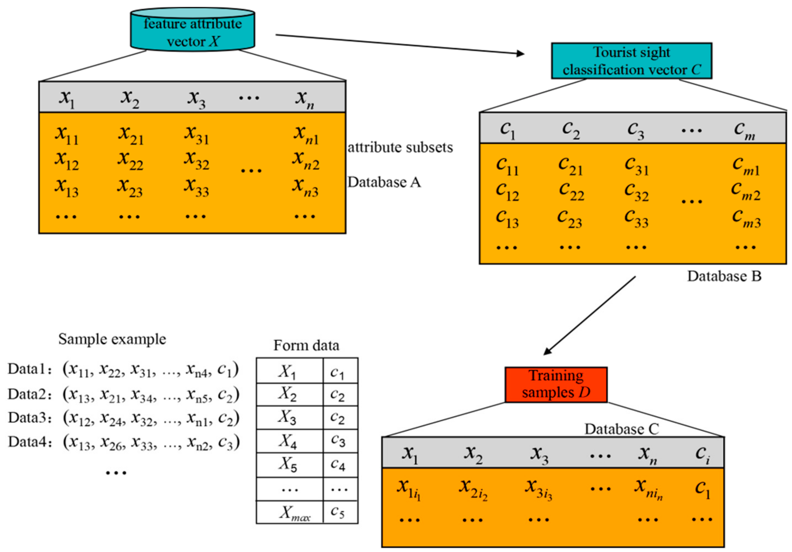
The tourist site of interest classification distribution matrix $A$ formed by the Naïve Bayes machine learning mining process is the critical model for smart machine to learn tourists’ needs and interests. In the matrix $A$, arbitrary row $\forall A_w$ represents one feasible sort of tourist site classification and quantity. Each row’s classification and quantity can meet the needs of tourists, but they differ in specific tourist sites, which will output different tour routes. According to the definition, as to one row $A_w$ of matrix $A$, the feasible sort of classification and quantity is ${\displaystyle {\prod }_{j=1}^m{C}_{s_j}^{a_{wj}}},s.t.a_{wj}\ne 0$, but not all the sorts are the optimal ones. The tourists start from temporary accommodation in the city, visit all selected tourist sites, and finally return to temporary accommodation, and the whole process forms an integrated tour route. The selected tourist sites should meet the needs and interests while costing the minimum expenditure. Thus, within the neighbourhood range of a temporary accommodation center, the nearer to the center, the more beneficial of the tourist site will be. Thus, in ${\displaystyle {\prod }_{j=1}^m{C}_{s_j}^{a_{wj}}}$, there are different sorts of tourist classifications and quantities and only one sort is optimal in geographic distribution. The membership degree relationship is used to set up the neighbourhood searching arc for the seed tourist site and to iterate the tourist sites to generate the propagating tree. The process of searching for subordinate seed tourist sites is in the range of one tourist site cluster or cross-cluster, that is, the tourist sites may belong to the same cluster or different clusters. The final output result of the process is a propagating tree with optimal geographic distributed tourist sites, and notes on the tree are the mined optimal tourist sites.

Definition 7.

Tourist site clustering center$K$. The temporary accommodation which is confirmed and checked in before the trip is set as the starting point and terminal point of the whole tour activity. The temporary accommodation is the first critical point of the planned tour route, which is called the tourist site clustering center$K$. The center$K$is determined by the temporary accommodation’s location, here defined as the longitude and latitude$(l,B)$.

The center $K$ will change with the tourist’s decision on the temporary accommodation and will directly influence the propagating tree’s formation, shape and distribution, and influence the mined optimal tourist sites.

Definition 8.

Seed tourist site$G_e$and seed tourist site vector$G_w$. Starting from tourist site clustering center$K$, searched and confirmed optimal tourist sites within neighbourhood via objective function and membership degree are called seed tourist site$G_e$. Under the condition of one sort of tourist site classification and quantity, the searched seed tourist sites for each tourist site classification$c_j$is$a_{wj}$, and${\displaystyle {\sum }_{j=1}^m{a}_{wj}},s.t.\forall w$,$e\in (0,{\displaystyle {\sum }_{j=1}^m{a}_{wj}}]\in {\mathrm{Z}}^{+}$ is the total quantity of seed tourist sites, according to the tourist site of interest classification distribution matrix $A$ and its arbitrary row vector $\forall A_w$. We store ${\displaystyle {\sum }_{j=1}^m{a}_{wj}}$ seed tourist sites in the sequence of the propagating tree’s nodes in the vector element from left to right in order, and this vector is called the seed tourist site vector $G_w$.

Under the condition of the confirmed tourist site clustering center $K$, matrix $A$ can generate $p$ seed tourist site vectors $G_w$, and $w\in (0,p]\in {\mathrm{Z}}^{+}$, according to the definition. Each $G_w$ stores the searched optimal tourist sites of row $A_w$.

Definition 9.

Subordinate seed tourist site$G_e^{\ast }$and non-subordinate seed tourist site$\neg G_e^{\ast }$. As to one seed tourist site$G_e$, the searched and confirmed tourist site which is closest to starting center$K$or seed tourist site$G_e$and it will be listed to store in propagating tree nodes via subordinate function and membership degree relationship model is called subordinate seed tourist site$G_e^{\ast }$. In the same searching process, other tourist sites that are not listed to store in propagating tree nodes are called non-subordinate seed tourist site$\neg G_e^{\ast }$.

Definition 10.

Seed tourist site searching arc. We set initial seed tourist site$G_e$as the circle center, and take the neighbourhood radius confirmed by the objective function as the arc. The arc is used to search the subordinate seed tourist site$G_e^{\ast }$. The combined structure of the radius and arc is called the seed tourist site searching arc. The seed tourist site searching arc is the direction and path to search the seed tourist site. In one searching process, a smart machine scans all of the tourist sites, and seed tourist site will be bound to pass the seed tourist site searching arc with a minimum objective function value.

Definition 11.

Optimal tourist site propagating tree$tre{e}_w$. The structure tree searched and confirmed by seed tourist sites and subordinate seed tourist site generation model is called the optimal tourist site propagating tree. The nodes of the optimal tourist site propagating tree are tourist sites, which are optimally geographic distributed, conform to tourists’ interests and feature attributes, and cost the least expenditure.

According to the definition, under the condition of the confirmed tourist site clustering center $K$, matrix $A$ can generate $p$ optimal tourist site propagating trees $tre{e}_w$, and $w\in (0,p]\in {\mathrm{Z}}^{+}$. The optimal tourist site mining algorithm that is based on the membership degree searching propagating tree is designed and developed, according to definition and the thought of optimal tourist site propagating tree modeling.

Step 1. Confirm the propagating tree universe of discourse

According to the definition of the tourist site classification vector $C$, as to one certain tourism city, the specific tourist site of No. $c_j$ tourist site classification is $c_{js}$. The tourist site quantity of $c_j$ is $s_j$, $s\in (0,s_j]\in {\mathrm{Z}}^{+}$.

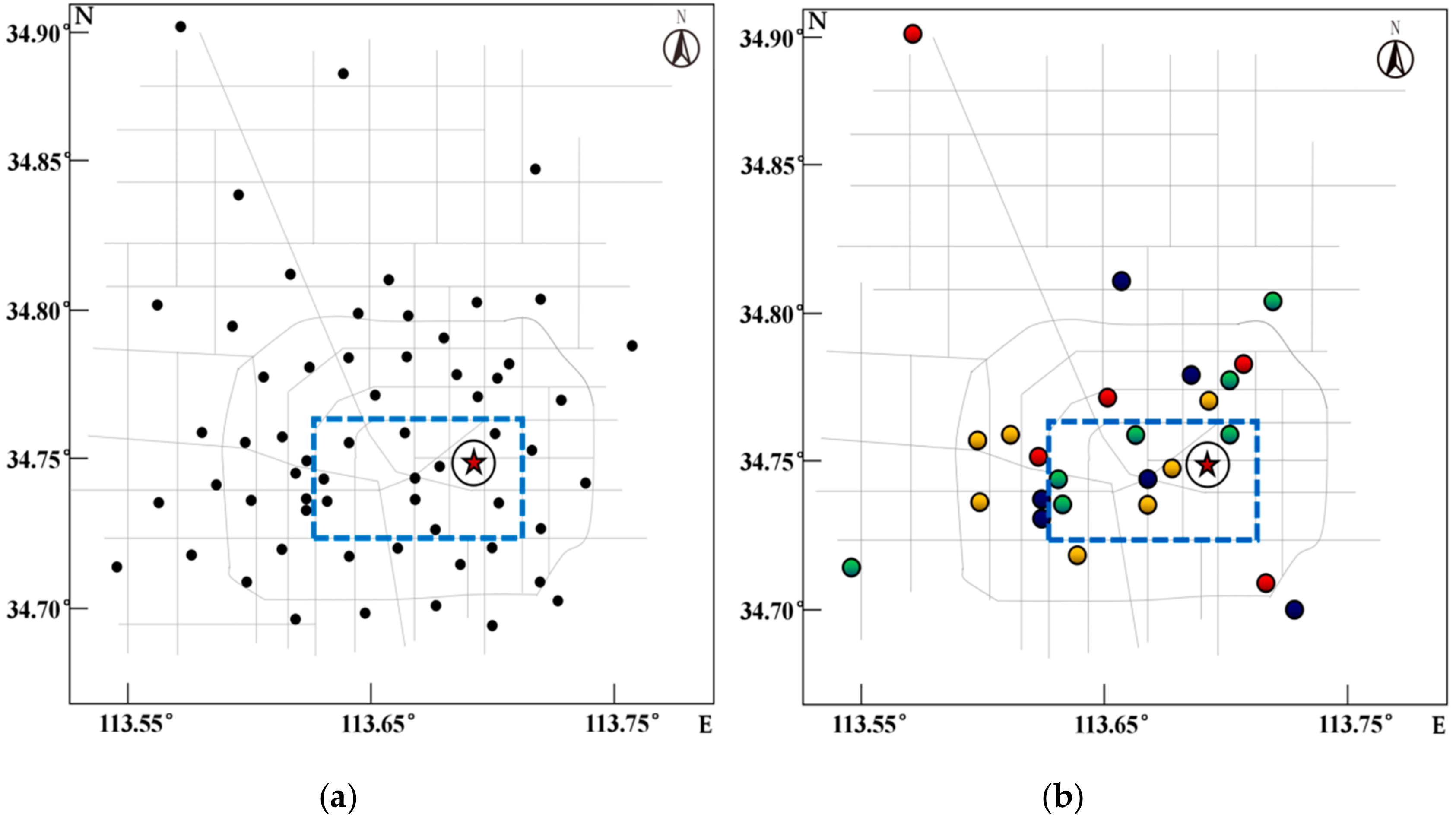
We set the city tourist site set as $C_s=\{c_{11},c_{12},\dots ,c_{1s_1},c_{21},c_{22},\dots ,c_{2s_2},\dots ,c_{m1},c_{m2},\dots ,c_{m{s}_m}\}\subset R^s$, which is called the universe of discourse. $c_{js}={(c_{js}^1,c_{js}^2,\dots ,c_{js}^u)}^{\mathrm{T}}\in R^s$ is the feature vector of samples to be observed, and it relates to one point of universe of discourse feature space, that is, the tourist site in city geographic space. $c_{js}^{\alpha }$ is the feature attribute value of No. $\alpha$ dimensions of feature vectors. As to the tourist site itself, feature attribute values contain the tourist site’s longitude $l$, tourist site’s latitude $B$, and tourist site’s attraction index $\epsilon$.

Step 2. Divide the propagating tree universe of discourse into clusters

Starting from the tourist site clustering center $K$, we divide the propagating tree universe of discourse into $m$ clusters $c_j$, and each division cluster $c_j$ relates to one tourist site classification, which forms a tourist site cluster $c_j$. Thus, the clusters of propagating tree universe of discourse are $c_1$, $c_2$, …, $c_m$, and they meet the formula (7) conditions.

$$\left\{\begin{array}{l}{c}_1\cup c_2\cup \dots \cup c_m=C\\ c_j\cap \forall c_{\neg j}=\varnothing ,s.t.j,\neg j\in (0,m]\subset {\mathrm{Z}}^{+}\\ c_j\ne \varnothing ,c_j\ne C,s.t.j\in (0,m]\subset {\mathrm{Z}}^{+}\end{array}\right.$$

(7)

In the process of searching seed tourist sites starting from the tourist site clustering center $K$, the searched subordinate seed tourist site $G_e^{\ast }$ and initial seed tourist site $G_e$ may be in the same classification cluster or in the different classification clusters, and the searching process should meet the constraint conditions. Here, the seed tourist sites in the same classification cluster are noted as $G_{e+}^{\ast }$, while in the different classification cluster, they are noted as $G_{e-}^{\ast }$.

Step 3. Set up the objective function and subordinate function

The space searching relationship of the tourist site clustering center $K$, seed tourist site $G_e$, and subordinate seed tourist site $G_e^{\ast }$ is determined by the clustering principle of $K$, $G_e$, and $G_e^{\ast }$. The principle is the second order Minkowski distance. According to the definition of tourist site feature attributes, the Minkowski distance between the tourist site clustering center $K$ and the first mined seed tourist site $G_1$, and the Minkowski distance between the seed tourist site $G_e$ and subordinate seed tourist site $G_e^{\ast }$ are determined by their feature attributes. Other than the tourist site’s longitude $l$, latitude $B$, and tourist site attraction index $\epsilon$, there exist factors that influence the process to search the subordinate seed tourist site.

Definition 12.

Membership degree direct influence factor${\lambda }_{v1}$. In the process of single searching, the factors that directly influence whether one certain tourist site is the subordinate seed tourist site$G_e^{\ast }$of initial seed tourist site$G_e$or not are called the membership degree direct influence factors${\lambda }_{v1}$,$v_1\in (0,\max v_1]\subset {\mathrm{Z}}^{+}$.

Definition 13.

Membership degree indirect influence factor${\delta }_{v2}$. In the process of single searching, the factors that indirectly influence whether one certain tourist site is the subordinate seed tourist site$G_e^{\ast }$of initial seed tourist site$G_e$or not are called the membership degree indirect influence factors${\delta }_{v2}$,$v_2\in (0,\max v_2]\subset {\mathrm{Z}}^{+}$.

The membership degree direct influence factors ${\lambda }_{v1}$ include the ferry distance between the tourist site clustering center $K$ and tourist site (km), the ferry distance between the two tourist sites (km), the quantity of subways and bus lines between the ferry interval, the taxi fee of the ferry interval and the road traffic jam index, according to the actual travel process and city tourism service. The membership degree indirect influence factors ${\delta }_{v2}$ include the quantity of traffic light between the tourist site clustering center $K$ and the tourist site, the quantity of traffic light between two tourist sites, the average walking distance from a tourist site to the nearest subway or bus station (km), the average waiting time for a taxi (h), and the average quantity of traffic jammed roads. According to definition, factor s ${\lambda }_{v1}$ and ${\delta }_{v2}$ are represented in text format. The symbol “$dir+$” stands for factors ${\lambda }_{v1}$, and the symbol “$indir-$” stands for factors ${\delta }_{v2}$. The text format is defined as <Factor, Relationship, Algorithm, Attribute>, and each factor is represented, as follows.

< Direct factor 1: <${\lambda }_1$, ferry distance, temporary accommodation → tourist site $S_1$ (km, $S_1\in {\mathrm{R}}^{+}$),

${\lambda }_1=S_1^{-1}$, $dir+$>;

Indirect factor 1: <${\delta }_1$, quantity of traffic light, temporary accommodation → tourist site $N_1$

($N_1\in {\mathrm{Z}}^{+}$), ${\delta }_1=-0.01N_1$, $indir-$>>

< Direct factor 2: <${\lambda }_2$, ferry distance, tourist site → tourist site $S_2$ (km, $S_2\in {\mathrm{R}}^{+}$), ${\lambda }_2=S_2^{-1}$, $dir+$>;

Indirect factor 2: <${\delta }_2$, quantity of traffic light, tourist site → tourist site $N_2$ ($N_2\in {\mathrm{Z}}^{+}$),

${\delta }_2=-0.01N_2$, $indir-$>>

< Direct factor 3: <${\lambda }_3$, quantity of subway and bus line $N_3$ ($N_3\in {\mathrm{Z}}^{+}$), ${\lambda }_3=0.1N_3$, $dir+$>

Indirect factor 3: <${\delta }_3$, ferry distance, tourist site → nearest subway or bus station $S_3$ (km,

$S_3\in {\mathrm{R}}^{+}$), ${\delta }_3=-0.01S_3$, $indir-$>>

< Direct factor 4: <${\lambda }_4$, taxi fee of ferry distance, $cost$ ($cost\in {\mathrm{R}}^{+}$), ${\lambda }_4=cos{t}^{-1}$, $dir+$>

Indirect factor 4: <${\delta }_4$, average waiting time of taxi, $t$ (h, $t\in {\mathrm{R}}^{+}$), ${\delta }_4=-0.01t$, $indir-$>>

< Direct factor 5: <${\lambda }_5$, road traffic jam index, $d$ ($d\in {\mathrm{R}}^{+}$), ${\lambda }_5=1-d$, $dir+$>

Indirect factor 5: <${\delta }_5$, average quantity of traffic jam, $N_4$ ($N_4\in {\mathrm{Z}}^{+}$), ${\delta }_5=-0.01N_4$, $indir-$>>.

According to the definition, the city tourist site set $C$ can be stored as a $u\times {\displaystyle {\sum }_{j=1}^m{s}_j}$ dimension matrix. The matrix’s columns relates to specific tourist sites, while the rows relates to the feature attribute. The feature attributes include the membership degree direct influence factors ${\lambda }_{v1}$, membership degree indirect influence factors ${\delta }_{v2}$, tourist site longitude $l$, tourist site latitude $B$, the tourist site attraction index $\epsilon$, and $\max u=\max v_1+\max v_2+3$. According to Definitions 12 and 13, factors ${\lambda }_{v1}$ and ${\delta }_{v2}$ of the tourist site clustering center $K$ and first searched seed tourist site, seed tourist site, and subordinate seed tourist site are determined by the tourist site clustering center $K$ and relative tourist sites, in which, if one point changes, the values of factors ${\lambda }_{v1}$ and ${\delta }_{v2}$ will change simultaneously, thus the values of factors ${\lambda }_{v1}$ and ${\delta }_{v2}$ are fluctuating. The objective function of the tourist site clustering center $K$ and first searched seed tourist site, seed tourist site, and subordinate seed tourist site are determined by feature attributes, as shown in formula (8).

$$\begin{array}{c}\left\{\begin{array}{l}\sigma (K,c_{js})={\sum }_{v_1=1}^{max{v}_1}{\lambda }_{v1}+{\sum }_{v_2=1}^{max{v}_2}{\delta }_{v2}+0.01{({(\Delta l_{K,c_{js}})}^2+{(\Delta B_{K,c_{js}})}^2)}^{-1/2}+|\Delta {\epsilon }_{K,c_{js}}|\\ \sigma (c_{js},c_{j^{\prime }{s}^{\prime }})={\sum }_{v_1^{{}^{\prime }}=1}^{max{v}_1^{{}^{\prime }}}{\lambda }_{v_1^{{}^{\prime }}}+{\sum }_{v_2^{{}^{\prime }}=1}^{max{v}_2^{{}^{\prime }}}{\delta }_{v_2^{{}^{\prime }}}+0.01{({(\Delta l_{c_{js},c_{j^{\prime }{s}^{\prime }}})}^2+{(\Delta B_{c_{js},c_{j^{\prime }{s}^{\prime }}})}^2)}^{-1/2}+|\Delta {\epsilon }_{c_{js},c_{j^{\prime }{s}^{\prime }}}|\\ J(\sigma (K,c_{js}),\sigma (c_{js},c_{j^{\prime }{s}^{\prime }}))=\sigma (K,c_{js})+\sigma (c_{js},c_{j^{\prime }{s}^{\prime }})\\ s.t.j\ne j^{\prime }ors\ne s^{\prime }\end{array}\right.\end{array}$$

(8)

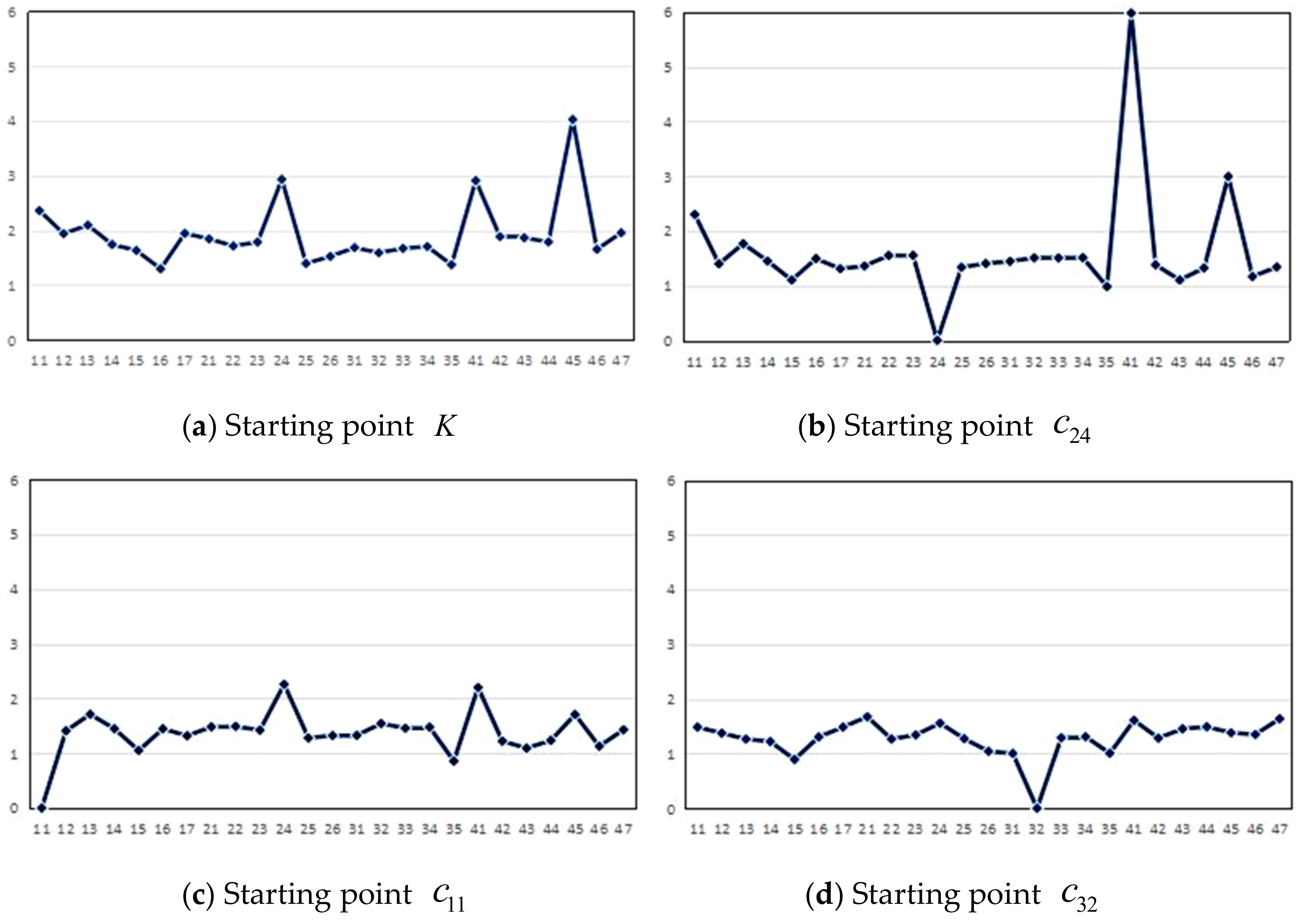
Definition 14.

Objective function descending order vector$Q$. In the process of single searching subordinate seed tourist site$G_e^{\ast }$, we store the searched objective function values in a vector in the sequence of elements from left to right in descending order, and this vector is called the objective function descending order vector$Q$.

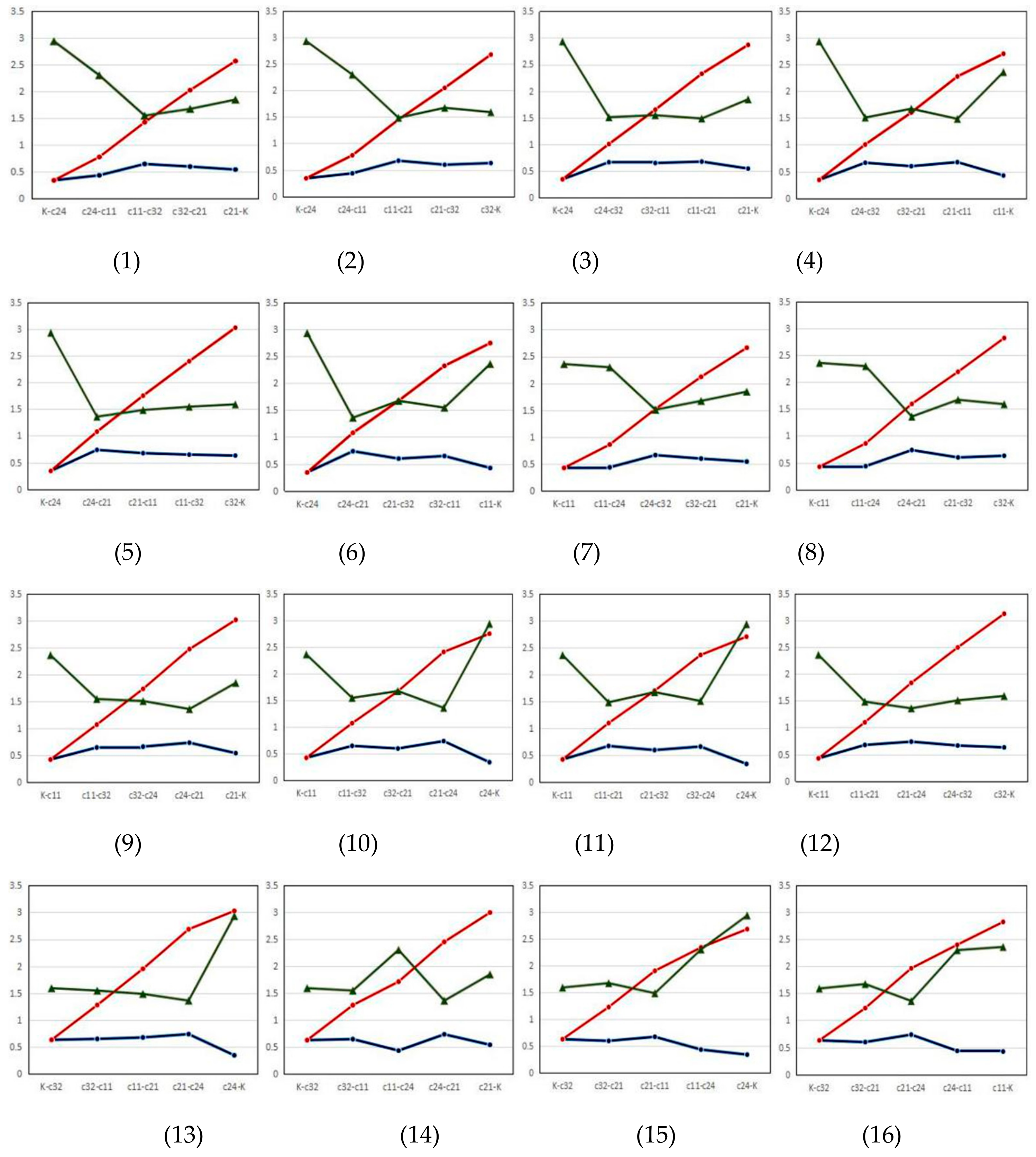
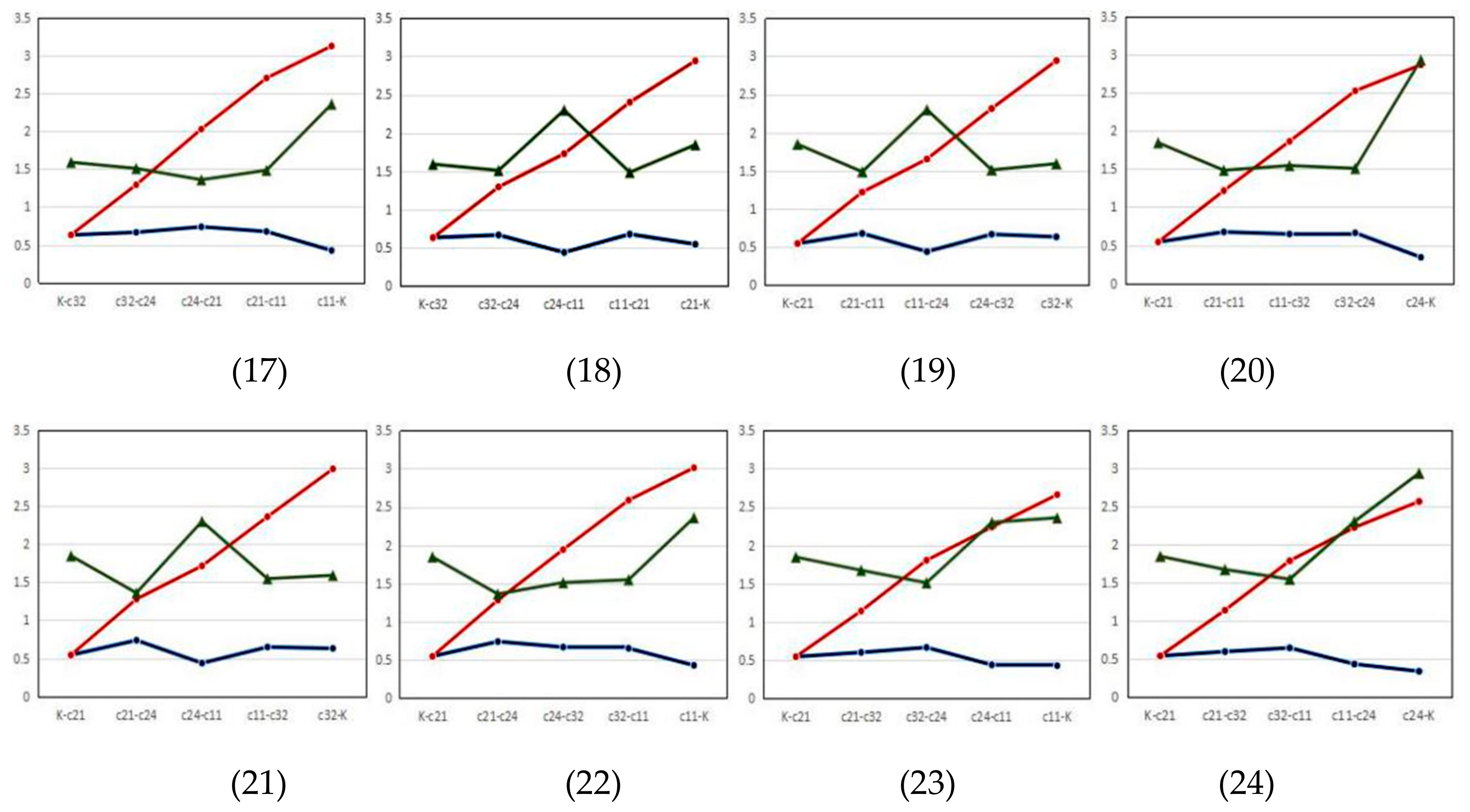
Definition 15.

Objective function fluctuating curve. In the process of single searching a subordinate seed tourist site $G_e^{\ast }$, the fluctuating curve, which reflects objective function values tendency, is called the objective function fluctuating curve.

The objective function fluctuating curve changes with the tourist site clustering center $K$ and the selected tourist site classification and quantity $A_w$. When $K$ or $A_w$ changes greatly, the objective function fluctuating curve tendency will also change greatly. In the process of searching the subordinate seed tourist site $G_e^{\ast }$ starting from the clustering center $K$ or seed tourist site $G_e$, in one time of searching, one group of objective function values will be generated. The objective function fluctuating curve visually reflects the affinities relationship between the seed tourist site and other tourist sites in one single searching process.

Definition 16.

Seed tourist site full rank for classification$c_j$. As to one certain nonzero tourist site classification$a_{wj}\ne 0$of tourist site classification and quantity$A_w$in matrix$A$, during the searching process, when the quantity of the searched seed tourist site for this classification reaches$a_{wj}$, the seed tourist site for the classification$c_j$is full rank under the condition of$A_w$, and it is noted as$c_j^{\wedge }$. When the seed tourist site for the classification is full rank, the propagating tree will not accept further searched seed tourist sites of the same classification.

One single searching process only confirms and mines one tourist site as the subordinate tourist site and, meanwhile, the other tourist sites are non-subordinate tourist sites. The subordinate function $\mu ((K,c_{js}),c_{j\prime s\prime })=\mu (K,c_{js})(c_{j\prime s\prime })$, which is noted by the membership degree that represents the subordinate relationship between tourist site $c_{j\prime s\prime }$ and initial seed tourist site $c_{js}$ or the tourist site clustering center $K$ in one single searching process. The subordinate function is formula (9).

$$\mu ((K,c_{js}),c_{j\prime s\prime })=\mu (K,c_{js})(c_{j\prime s\prime })=\left\{\begin{array}{l}1, condition1\\ 0, condition2\end{array}\right.$$

(9)

Definition 17.

Membership degree distribution matrix$\mu (c)$. When the tourist site$c_{j\prime s\prime }$is the subordinate seed tourist site for the clustering center$K$or initial seed tourist site$c_{js}$, the membership degree value of tourist site$c_{j\prime s\prime }$is 1, or the value is 0. One single searching process can confirm one tourist site’s membership degree value as 1, and other tourist sites’ values as 0. The matrix that represents the subordinate relationship of all tourist sites via subordinate function values is called the membership degree distribution matrix$\mu (c)$.

As shown in formula (10), it represents the distribution of seed tourist sites. The matrix row is one sort of tourist site classification and quantity. The matrix column is the membership degree of the No. $s$ tourist site for the sort of tourist site classification and quantity. The quantity of column is $\max s_j$, and vacant elements are noted as 0. When the clustering center $K$ or $A_w$ changes, the membership degree distribution matrix will also change.

$$\mu (c)=\left(\begin{array}{ccccc}\mu (c_{11})& \mu (c_{12})& \mu (c_{13})& \dots & \mu (c_{1s1})\\ \mu (c_{21})& \mu (c_{22})& \mu (c_{23})& \dots & \mu (c_{2s2})\\ & & \dots & & \\ \mu (c_{m1})& \mu (c_{m2})& \mu (c_{m3})& \dots & \mu (c_{msm})\end{array}\right)$$

(10)

Step 4. Set up the optimal tourist site mining algorithm

Objective function descending order vector $Q$ stores objective function values. If the tourist site classification relating to the first element of objective function value is not full rank and not listed in the previous seed tourist sites, and then the tourist site relating to the objective function value is mined as subordinate seed tourist site $G_e^{\ast }$ of the tourist site clustering center $K$ or initial seed tourist site $G_e$, if in the same cluster, note it as $G_{e+}^{\ast }$, if in the different cluster, we note it as $G_{e-}^{\ast }$. Tourist sites relating to the objective function values on other elements are non-subordinate seed tourist sites $\neg G_e^{\ast }$. Starting from the clustering center $K$, the process of searching the seed tourist site vector $G_w$ and obtaining the objective function descending order vector $Q$, as well as the membership degree distribution matrix $\mu (c)$ is as follows.

Sub-step 1. Confirm matrix $A$. The tourist selects one sort of tourist site classification and quantity vector $A_w$.

Sub-step 2. We set up $1\times {\displaystyle {\sum }_{j=1}^m{a}_{wj}}$ dimension seed tourist site vector $G_w$, $1\times {\displaystyle {\sum }_{j=1}^m{s}_j}$ dimension objective function descending order vector $Q$ and $m\times \max s_j$ dimension membership degree distribution matrix, and set all elements as 0.

Sub-step 3. We set up the Open list and Closed list. The open list is used to store all non-seed tourist sites to be searched. The Closed list is used to store all searched seed tourist sites. The storage format of the Open list and Closed list is the same as the tourist site classification vector $C$, and the elements for the two lists are set in the sequence of the tourist site classification and order. The Open list and Closed list contain ${\displaystyle {\sum }_{j=1}^m{s}_j}$ elements, respectively, according to the definition. We store all elements of the city tourist site set $C_s$ in the Open list.

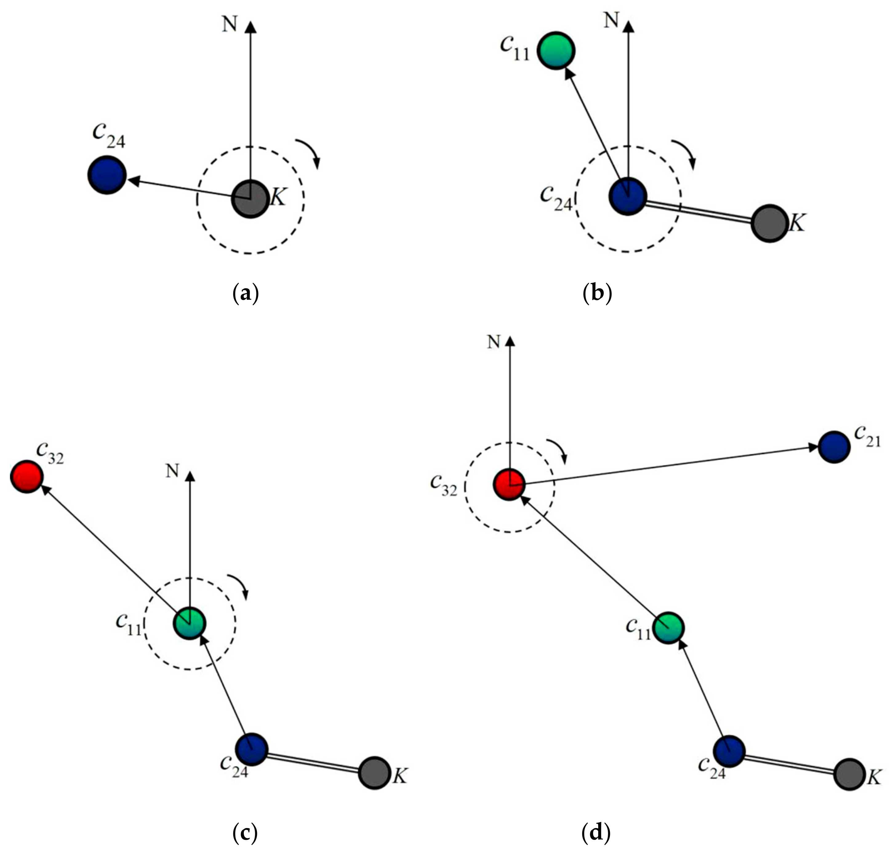
Sub-step 4. Search and confirm the No.1 seed tourist site $G_1$. Here is the definition of seed tourist site searching angle.

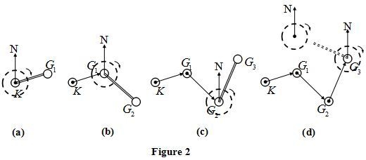
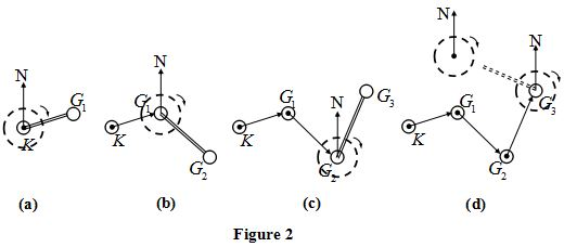
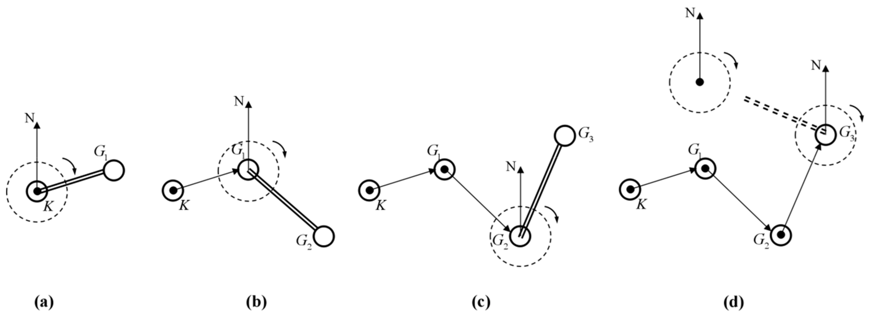
Definition 18.

Seed tourist site searching angle$\phi$. Starting from one certain central point, we draw a ray$l_1$directing to the geographic north and another ray$l_2$connecting with the central point and another point. The included angle from the north ray$l_1$to ray$l_2$in a clockwise direction is called the searching angle. If the central point is the clustering center$K$or initial seed tourist site$G_e$, the other point is one tourist site$c_{js}$to be searched, and the included angle from the ray of the clustering center$K$or initial seed tourist site$G_e$to the ray of the tourist site$c_{js}$is called the seed tourist site searching angle$\phi$, noted as$\phi (K,c_{js})$or$\phi (G_e,c_{js})$.

The process of searching the No.1 seed tourist site is as follows.

(I) The clustering center $K$ is set as the central point to confirm the ${\displaystyle {\sum }_{j=1}^m{S}_j}$ searching angle $\phi (K,c_{11})$, $\phi (K,c_{12})$, …, $\phi (K,c_{m{s}_m})$ for tourist sites;

(II) search and calculate the objective function value $\sigma (K,c_{11})$ in the direction of the searching angle $\phi (K,c_{11})$ and objective function value $\sigma (K,c_{12})$ in the direction of the searching angle $\phi (K,c_{12})$;

① if $\sigma (K,c_{11})\ge \sigma (K,c_{12})$, store $\phi (K,c_{11})$ into the first element of vector $Q$, and store $\phi (K,c_{12})$ into the second element of vector $Q$;

② if $\sigma (K,c_{11})<\sigma (K,c_{12})$, store $\phi (K,c_{12})$ into the first element of vector $Q$, and store $\phi (K,c_{11})$ into the second element of vector $Q$;

(III) search and calculate the objective function value $\sigma (K,c_{13})$ on the direction of the searching angle $\phi (K,c_{13})$:

① if $\sigma (K,c_{11})\ge \sigma (K,c_{12})\ge \sigma (K,c_{13})$, keep the first and second element unchanged, and store $\sigma (K,c_{13})$ into the third element of vector $Q$;

② if $\sigma (K,c_{11})\ge \sigma (K,c_{13})\ge \sigma (K,c_{12})$, keep the first element unchanged, and descend $\sigma (K,c_{12})$ to the third element of vector $Q$;

③ if $\sigma (K,c_{13})\ge \sigma (K,c_{11})\ge \sigma (K,c_{12})$, descend $\sigma (K,c_{11})$ and $\sigma (K,c_{12})$ to the second and third elements of vector $Q$, and ascend $\sigma (K,c_{13})$ to the first element of vector $Q$; and,

④ as to $\sigma (K,c_{11})<\sigma (K,c_{12})$, the comparison method of $\sigma (K,c_{13})$ and other two values is the same as step (III) sub-steps ①–③.

(IV) Return to step (I)–(III) and continue searching and comparing the objective function values of other searching angles, store the function values into vector $Q$, and finally find the objective function descending order vector $Q_1$ and objective function fluctuating curve $curv{e}_1$ searched by the central point of the clustering center $K$.

(V) Extract the first element value of vector $Q_1$, and its searching angle’s related tourist site is $Q_{11}$. Enter the following judgment steps:

① Search the Closed list. If $Q_{11}$ appears in the Closed list, jump to the second element $Q_{12}$ of vector $Q_1$;

② If $Q_{12}$ appears in the Closed list, continue to jump to the third element $Q_{13}$ of vector $Q_1$;

③ Start searching from tourist site $Q_{11}$, according to the method of step (V) sub-steps ① and ②, if tourist site $Q_{1v_1}$ appears in the Closed list, continue searching; if one certain tourist site $Q_{1v_1}$ does not appear in the Closed list, then jump to step ④, $v_1\in (0,{\displaystyle {\sum }_{j=1}^m{s}_j}]\subset {\mathrm{Z}}^{+}$;

④ Judge and confirm the tourist site classification $c_j$ for tourist site $Q_{1v_1}$:

(i) If the tourist site classification $c_j$ is not full rank $\neg c_j^{\wedge }$, and then confirm tourist site $Q_{1v_1}$, as the No.1 seed tourist site $G_1$ and store it into the first element of the seed tourist site vector $G_w$. Confirm the seed tourist site’s membership degree to the clustering center $K$ is 1. The other tourist sites’ membership degrees are all 0. Store $G_1$ into the Closed list and delete $G_1$ from the Open list; and,

(ii) If the tourist site classification $c_j$ is full rank $c_j^{\wedge }$, return to step (V) sub-steps ①–③ and search the next tourist site $Q_{1v_2}$ which does not appear in the Closed list. Enter the judgment of step (V) sub-step ④. Repeat the process until the seed tourist seed is searched and confirmed, and then store it into the first element of vector $G_w$.

Sub-step 5. Search and confirm the No.2 seed tourist site and subsequent seed tourist sites.

(I) According to Sub-step 4, set the initial seed tourist site $G_1$ as the central point. Search the No.2 seed tourist site $G_2$ in the whole geographic range and store it into vector. Confirm the membership degree of the seed tourist site to initial seed tourist site $G_1$ as 1, other tourist sites’ membership degrees as set as 0. Store $G_2$ into the Close list, and delete it from the Open list;

① If the tourist site classification for the seed tourist site $G_1$ is not full rank $\neg c_j^{\wedge }$, that is, $G_1$ and $G_2$ are in the same cluster, note $G_2$ as $G_{1+}^{*}$; and,

② If the tourist site classification for the seed tourist site $G_1$ is full rank $c_j^{\wedge }$, that is, $G_1$ and $G_2$ are in two different clusters, note $G_2$ as $G_{1-}^{*}$.

(II) Set the initial seed tourist site $G_2$ as the central point. Search the No.3 seed tourist site $G_3$ in the whole geographic range and store it into vector. Confirm the membership degree of the seed tourist site to initial seed tourist site $G_2$ as 1, and set the other tourist sites’ membership degrees as set as 0. Store $G_3$ into the Close list, and delete it from the Open list. The method to note the $G_3$ cluster is the same as Sub-step 5 step (I); and,

(III) According to Sub-step 5 step (I) and (II), search and store subsequent seed tourist sites until each tourist site of interest classification $c_j$ gets to full rank $c_j^{\wedge }$, $j=1,2,\dots ,m$, and also the seed tourist site vector $G_w$ is full rank. The method to note cluster is the same as Sub-step 5 step (I). In the process of searching the seed tourist site, the objective function descending order vector and objective function curve relating to each seed tourist site are also obtained. 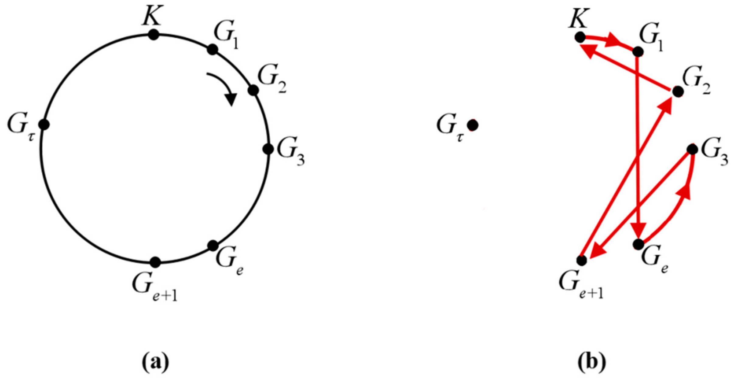Figure 2 shows the process of searching and mining subordinate seed tourist sites with previously searched seed tourist sites as the central points.

Step 5. Generate the optimal tourist site propagating tree

Starting from the clustering center $K$, generate the optimal tourist site propagating tree in the sequence of the seed tourist site vector $G_w$ element. This tree is the tendency of optimal tourist sites that meet tourists’ needs and interests and have the optimal geographic distribution. It is also the visualized process for a smart machine to output the optimal tourist sites according to the selected tourist classification and quantity.

Step 6. Generate the membership degree distribution matrix $\mu (c)$.

Based on the searched seed tourist site vector $G_w$, the membership degree distribution matrix $\mu (c)$ is generated. This matrix can intuitively reflect the quantity of the seed tourist sites as well as their distribution of each tourist site classification.

3.2. Tour Route Planning Algorithm Modeling based on Optimal Closed-loop Structure

The smart machine automatically plans optimal tour routes that meet tourists’ best motive benefits, according to the tourists’ interests learned from the Naïve Bayes machine learning module and optimal tourist sites searched by the membership degree searching propagating tree. All of the designed and developed algorithms are based on one-day trips. Within one day, the smart machine confirms no more than five optimal tourist sites for tourists and ensures that all of the mined tourist sites not only meet tourists’ needs and interests, cost the least expenditure with the optimal geographic distribution, but also consider tourists’ physical conditions, which helps tourists to have sufficient time to visit all the recommended tourist sites. Starting from temporary accommodation $K$, the whole trip of ferrying from one tourist site to another and visiting each tourist site and then returning to $K$ is an integrated closed-loop process, in which the quantity of visited optimal tourist sites is set as $\tau$, being noted as $\tau ={\displaystyle {\sum }_{j=1}^m{a}_{wj}}$, $\tau \in (0,5]\subset {\mathrm{Z}}^{+}$. Under the condition of confirmed $K$, there will be ${\mathrm{A}}_{\tau }^{\tau }$ sorts of tour routes, but not all of the tour routes can meet the tourists’ best motive benefits, there should be optimal ones and sub-optimal ones. The optimal ones will be the first important recommendation to tourists, while the sub-optimal ones will also be recommended to tourists. The attraction and motive benefits of one tour route for tourists depends on the influence of all the factors on the tour route, including factors ${\lambda }_{v1}$ and ${\delta }_{v2}$ in the actual trip, which are extracted to set up the objective function $J(\sigma (K,c_{js}),\sigma (c_{js},c_{j\prime s\prime }))$.

Definition 19.

Generation tree of the closed-loop structure$O_{\omega }$. Starting from the temporary accommodation$K$, the whole trip of ferrying from one tourist site to another and visiting each tourist site and then returning to$K$is an integrated closed-loop structure, and this structure is called a generation tree closed-loop structure$O_{\omega }$.

According to the quantity of tourist sites $\tau$, the ${\mathrm{A}}_{\tau }^{\tau }$ quantity of closed-loop structures can be confirmed, $\omega \in (0,{\mathrm{A}}_{\tau }^{\tau }]\subset {\mathrm{Z}}^{+}$, $\tau \in (0,5]\subset {\mathrm{Z}}^{+}$. One closed-loop structure relates to one tour route generation tree.

Definition 20.

Generation tree sub-unit$H(\cdot )$. In the whole trip process of one closed-loop structure, tourists will pass$\tau +1$independent ferry intervals, and each ferry interval is called generation tree sub-unit$H(\cdot )$.

According to the closed-loop structure, the ferry interval between $K$ and tourist, between two tourist sites, and between tourist site and $K$ are noted as $H(K,G_e)$, $H(G_e,G_{e+1})$, and $H(G_e,K)$. A generation tree sub-unit is the basic unit structure to output a sub-unit motive function value and generation tree motive function value. Here, it is defined that generation tree sub-units are independent from each other; tourists’ motive benefit obtained in one sub-unit has no relationship with another sub-unit.

Definition 21.

Sub-unit motive function$I(\cdot )$. In each sub-unit, the function is designed with the same initial motive iteration value$I_0$to iterate with the membership degree direct influence factors${\lambda }_{v1}$and indirect influence${\delta }_{v2}$and output motive iteration value of independent interval$H(\cdot )$. This function is called the sub-unit motive function$I(\cdot )$, as shown in formula (11).

The sub-unit motive function $I(\cdot )$ reflects the motive benefits of the ferry interval. The higher the function value is, the bigger the influence of factors on motive benefits will be, and the more satisfaction tourists will have. In the ferry interval of a sub-unit, the motive function $I(\cdot )$ is a monotone increasing function whose values will increase with tourists ferry distance increases. It finally outputs a maximum value of the interval, which is the sub-unit motive function $I(\cdot )$ value. Different sub-units have different function values, thus the whole trip’s sub-unit motive function $I(\cdot )$ values fluctuate with distance. Sub-unit motive function $I(\cdot )$ value has the feature of non-direction, that is, in the same sub-unit, function $I(\cdot )$ value remains unchanged back and forth.

$$\left\{\begin{array}{l}I(K,G_e)={\displaystyle {\sum }_{v_1=1}^{\max v_1}{I}_0{\lambda }_{v1}}+{\displaystyle {\sum }_{v_2=1}^{\max v_2}{I}_0{\delta }_{v2}}+I_0{({(\Delta l_{K,G_e})}^2+{(\Delta B_{K,G_e})}^2)}^{-1/2}+I_0|\Delta {\epsilon }_{K,G_e}|\\ I(G_e,G_{e\prime })={\displaystyle {\sum }_{v_1^{\prime }=1}^{\max v_1^{’}}{I}_0{\lambda }_{v_1^{\prime }}}+{\displaystyle {\sum }_{v_2^{\prime }=1}^{\max v_2^{\prime }}{I}_0{\delta }_{v_2^{\prime }}}+I_0{({(\Delta l_{G_e,G_{e’}})}^2+{(\Delta B_{G_e,G_{e’}})}^2)}^{-1/2}+I_0|\Delta {\epsilon }_{G_e,G_{e\prime }}|\\ I(G_e,K)={\displaystyle {\sum }_{v_{{}_1}^{″}=1}^{\max v_{{}_1}^{″}}{I}_0{\lambda }_{v_1^{″}}}+{\displaystyle {\sum }_{v_{{}_2}^{″}=1}^{\max v_{{}_2}^{″}}{I}_0{\delta }_{v_2^{″}}}+I_0{({(\Delta l_{G_e,K})}^2+{(\Delta B_{G_e,K})}^2)}^{-1/2}+I_0|\Delta {\epsilon }_{G_e,K}|\end{array}\right.$$

(11)

Definition 22.

Sub-unit motive weight$h(\cdot )$. The reciprocal of the sub-unit motive function$I(\cdot )$value is defined as the sub-unit motive weight$h(\cdot )$. The sub-unit motive weight$h(\cdot )$is the edge weight for two connecting point in the closed-loop. It is used as an edge weight parameter to search the optimal closed-loop structure.

According to the definition, the sub-unit motive weight $h(\cdot )$ meets formula (12). The sub-unit motive weight $h(\cdot )$ also has the non-direction feature. Thus, the graph that is composed by the clustering center $K$ and seed tourist sites $G_e$ is connected and non-direction graph.

$$h(K,G_e)=\frac{1}{I_{(K,G_e)}},\begin{array}{c}\end{array}h(G_e,G_{e\prime })=\frac{1}{I(G_e,G_{e\prime })},\begin{array}{c}\end{array}h(G_e,K)=\frac{1}{I(G_e,K)}$$

(12)

Definition 23.

Generation tree weight function$L(\cdot )$. The function which is iterated by the$\tau +1$sub-unit motive weight$h(\cdot )$and reflects the motive benefits of one generation tree closed-loop’s tour route is called the generation tree weight function$L(\cdot )$, as shown in formula (13). One generation tree weight function$L(\cdot )$relates to one tour route, and the lower the function value is, the more motive benefits the tourists will get from the tour route.

According to definition, in one closed-loop structure, the generation tree weight function $L(\cdot )$ is a monotone increasing function whose value increases with tourists’ ferrying distance increases, and finally outputs a maximum value. ${\mathrm{A}}_{\tau }^{\tau }$ function $L(\cdot )$ values are the elements for generation tree weight function minimum heap.

$$\left\{\begin{array}{l}L(K,K)=h(K,G_e)+{\displaystyle {\sum }_{e=1}^{\tau }h(G_e,G_{e\prime })}+h(G_e,K)\\ s.t.\begin{array}{c}\end{array}\forall |e\prime -e|\in (0,\tau -1]\subset {\mathrm{Z}}^{+}\end{array}\right.$$

(13)

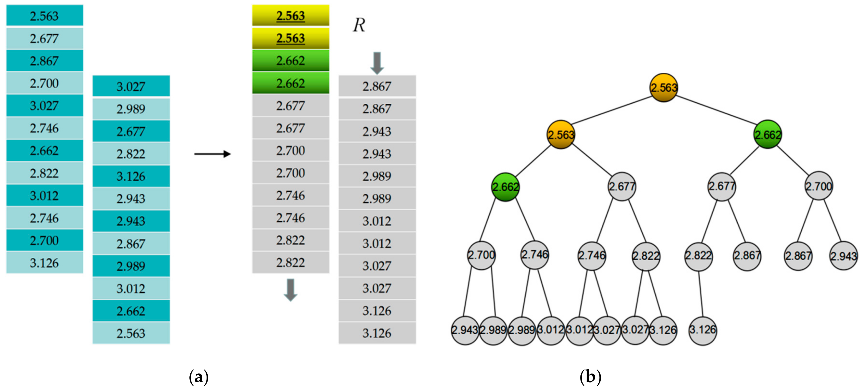
Definition 24.

Generation tree weight function minimum heap$R$. The minimum heap, which is formed by generation tree weight function values stored as array elements, is called the generation tree weight function minimum heap$R$.

According to the seed tourist site quantity $\tau$ and generation tree quantity ${\mathrm{A}}_{\tau }^{\tau }$, the minimum heap meets the following conditions:

(1) it contains ${\mathrm{A}}_{\tau }^{\tau }$ elements;

(2) set $n={\mathrm{A}}_{\tau }^{\tau }$, its element serial numbers $k_1$, $k_2$, …, $k_n$ meet: $k_i\le k_{2i}$, $k_i\le k_{2i+1}$,$1\le i\le ⌊n/2⌋$;

(3) the level of parent node is No.0. The height of the tree is $d$, and the other nodes are either on the No. $d$ level or on the No. $d-1$ level;

(4) when $d\ge 1$, there are $2^{d-1}$ nodes on the No. $d-1$ level;

(5) the branch nodes of the No. $d-1$ level all gather on the left of the tree;

(6) element value of each node is smaller than its child nodes; and,

(7) of all the node elements in the same level, left element is smaller than the right one.

According to the the definition, tour route planning algorithm modeling that is based on optimal closed-loop structure is set up. The basic thought is, motive weights between clustering center $K$ and each seed tourist site $G_e$, seed tourist site $G_e$, and seed tourist site $G_{e\prime }$ are confirmed by sub-unit motive function. By searching the ${\mathrm{A}}_{\tau }^{\tau }$ generation tree weight function values, a minimum heap sorting algorithm is used to confirm the minimum heap with weight function values in ascending order, and finally confirm the optimal tour routes and sub-optimal tour routes. The specific steps for the algorithm are as follows.

Step 1. Confirm the algorithm parameters:

(I) Confirm ${\lambda }_{v1}$ and ${\delta }_{v2}$. Extract the basic geographic information data of a certain tourism city and confirm the membership degrees direct influence factors ${\lambda }_{v1}$ and indirect influence factors ${\delta }_{v2}$ between the clustering center $K$ and each seed tourist site, seed tourist site $G_e$, and seed tourist site $G_{e\prime }$;

(II) Confirm $l$, $B$ and $\epsilon$. Extract the basic geographic information data and confirm the longitude and latitude coordinates $(l,B)$ of the clustering center $K$ and each seed tourist site $G_e$. Mine the tourism data information and obtain tourist site attraction indexes. Set the attraction index of the clustering center $K$ as ${\epsilon }_K=0$, as it is the starting point of the tour route.

Step 2. Iterate and calculate the sub-unit motive function values. From formula (11), the ${\mathrm{C}}_{\tau +1}^2$ motive function $I(\cdot )$ values between the clustering center $K$ and each seed tourist site $G_e$, seed tourist site $G_e$, and seed tourist site $G_{e\prime }$.

Sub-step 1 Confirm the $\tau$ motive function values between the clustering center $K$ and each seed tourist site $G_e$. The clustering center $K$ is the starting point and terminal point of the tour route;

Sub-step 2. Confirm ${\mathrm{C}}_{\tau }^2$ motive function values between arbitrary two seed tourist sites.

Step 3. Confirm the sub-unit motive weight. According to the sub-unit motive function values, confirm the ${\mathrm{C}}_{\tau +1}^2$ sub-unit motive weights between the clustering center $K$ and each seed tourist site $G_e$, seed tourist site $G_e$, and seed tourist site $G_{e\prime }$. The motive weight value is the edge weight of the connected and non-direction graph composed of the clustering center $K$ and each seed tourist site $G_e$.

Step 4. Search generation tree weight function minimum heap $R$. Through an edge correcting method to search the ${\mathrm{A}}_{\tau }^{\tau }$ generation tree weight function values relating to ${\mathrm{A}}_{\tau }^{\tau }$ generation tree closed-loop’s tour routes. Search and obtain the generation tree weight function minimum heap $R$ sorted by the generation tree weight function values in array via a sorting algorithm.

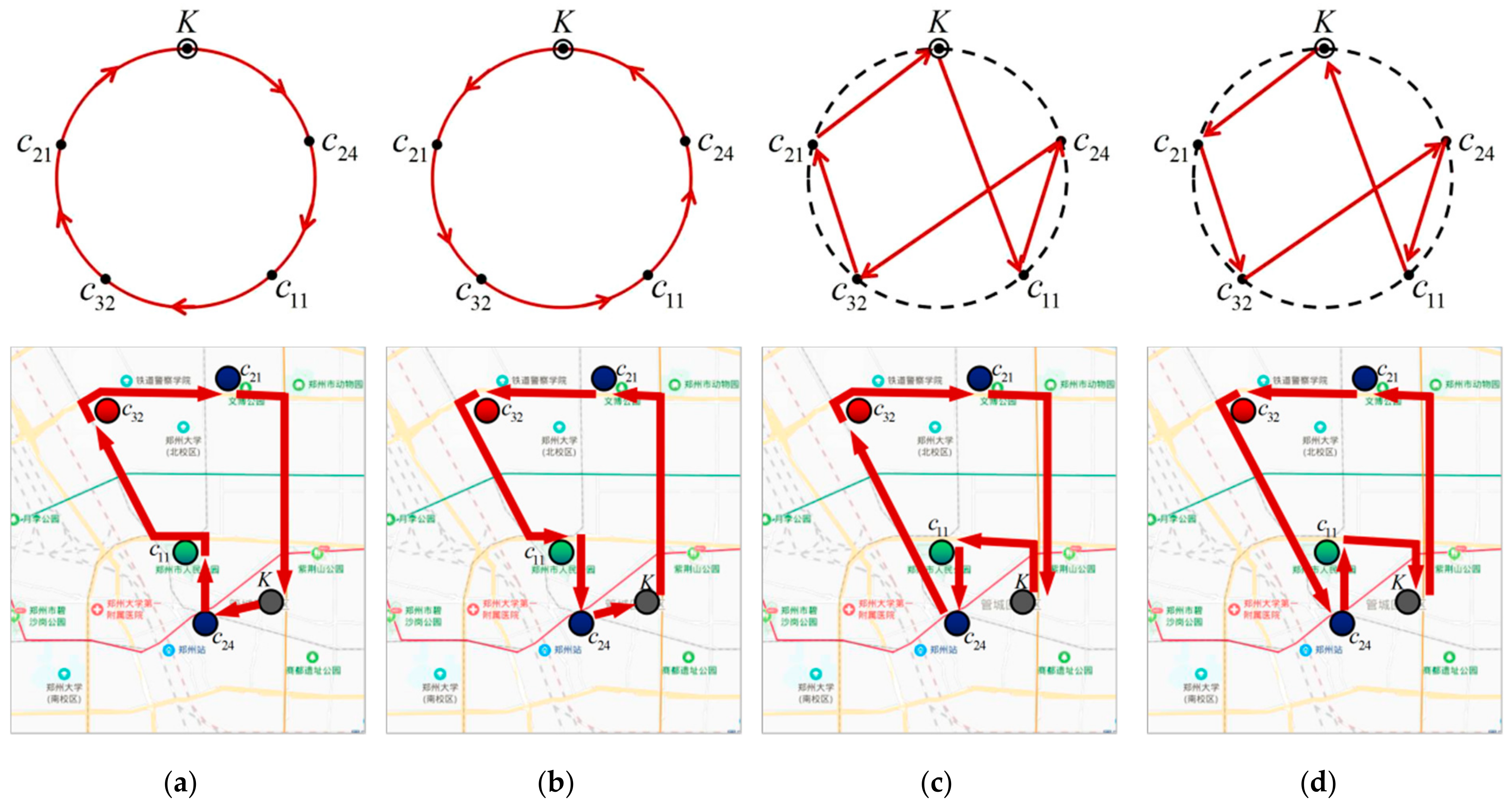
Sub-step 1. Set up a generation tree basic structure loop. Define a virtual closed-loop circle and evenly place points of the clustering center $K$ and all seed tourist sites $G_e$ on the circle. The connecting arc or line between two points can be clipped or connected in accordance with algorithm conditions, as shown in Figure 3. For the convenience of setting up the algorithm, note the clustering center $K$ as $v_1$, seed tourist site $G_1$ as $v_2$, and son on, and the seed tourist site $G_{\tau }$ as $v_{\tau +1}$.

Sub-step 2. Search the initial generation tree closed-loop structure $O_1$, and set:

$O_1=v_1,v_2,\dots ,v_i,\dots ,v_j,\dots ,v_{\tau +1},v_1$, $1<i\le j<\tau +1$, and $i,j,\tau \in {\mathrm{Z}}^{+}$.

(I) in structure $O_1$, search the $\tau +1$ sub-unit motive weights $h(\cdot )$ of adjacent $v_i$ and $v_{i+1}$;

(II) iterate the generation tree weight function value $L_1(K,K)$ of the closed-loop structure $O_1$; and,

(III) store the weight function value $L_1(K,K)$ into the parent node $R_1$ of minimum heap $R$.

Sub-step 3. Search the next generation tree closed-loop structure $O_2$. Find $\forall i,j$ and $i,j$ meet the following conditions:

(1) $1<i+1<j<\tau +1$;

(2) $h(v_i,v_j)+h(v_{i+1},v_{j+1})<h(v_i,v_{i+1})+h(v_j,v_{j+1})$.

Clip and rebuild the closed-loop structure $O_1$:

(I) delete sub-unit $H(v_i,v_{i+1})$ in $O_1$;

(II) delete sub-unit $H(v_j,v_{j+1})$ in $O_1$;

(III) add sub-unit $H(v_i,v_j)$; and,

(IV) add sub-unit $H(v_{i+1},v_{j+1})$.

The structure of the rebuilt generation tree closed-loop is:

$O_2=v_1,v_2,\dots ,v_i,v_j,v_{j+1},\dots ,v_{i+1},v_{j+1},v_{j+2},\dots ,v_{\tau +1},v_1$. Search the weight function value of generation tree closed-loop structure $O_2$.

(V) In structure $O_2$, search the $\tau +1$ sub-unit motive weights $h(\cdot )$ of adjacent $v_i$ and $v_{i+1}$;

(VI) iterate the generation tree weight function value $L_2(K,K)$ of the closed-loop structure $O_2$; and,

(VII) compare the generation tree weight function value $L_1(K,K)$ and $L_2(K,K)$, and update the generation tree weight function minimum heap $R$:

① If $L_1(K,K)\le L_2(K,K)$:

(i) keep the weight function value $L_1(K,K)$ storing in the parent node $R_1$ of minimum heap $R$ unchanged; and,

(ii) store the weight function value $L_2(K,K)$ into the child node $R_2$ of parent node $R_1$ in minimum heap $R$.

② If $L_1(K,K)>L_2(K,K)$:

(i) delete the parent node $R_1$ value $L_1(K,K)$; and,

(ii) store the weight function value $L_2(K,K)$ into the parent node $R_1$ in minimum heap $R$; and,

(iii) store the weight function value $L_1(K,K)$ into the child node $R_2$ of parent node $R_1$ in minimum heap $R$.

Sub-step 4. Return to Sub-step 3 and use the same method to search the next generation tree closed-loop structure $O_3$.

(I) in structure $O_3$, search $\tau +1$ sub-unit motive weights $h(\cdot )$ of adjacent $v_i$ and $v_{i+1}$;

(II) iterate the generation tree weight function value $L_3(K,K)$ of the closed-loop structure $O_3$; and,

(III) compare the generation tree weight function values $L_1(K,K)$, $L_2(K,K)$ and $L_3(K,K)$, and then update the generation tree weight function minimum heap $R$:

① If $L_1(K,K)\le L_2(K,K)$:

(i) if $L_1(K,K)\le L_2(K,K)\le L_3(K,K)$, keep the weight function values $L_1(K,K)$ and $L_2(K,K)$ storing unchanged, store the weight function value $L_3(K,K)$ into the child node $R_3$ of parent node $R_1$ in minimum heap $R$;

(ii) if $L_1(K,K)\le L_3(K,K)<L_2(K,K)$, keep the weight function value $L_1(K,K)$ storing unchanged, delete the child node $R_2$ value and store the weight function value $L_3(K,K)$ into the child node $R_2$ of parent node $R_1$, store the weight function value $L_2(K,K)$ into the child node $R_3$ of parent node $R_1$ in minimum heap $R$; and,

(iii) if $L_3(K,K)<L_1(K,K)\le L_2(K,K)$, delete the child node $R_1$ and $R_2$ values, store the weight function value $L_3(K,K)$ into the parent node $R_1$. Store the weight function value $L_1(K,K)$ and $L_2(K,K)$ into the child node $R_2$ and $R_3$ of parent node $R_1$ respectively in minimum heap $R$.

② If $L_1(K,K)>L_2(K,K)$:

(i) if $L_3(K,K)\ge L_1(K,K)>L_2(K,K)$, keep the weight function values $L_1(K,K)$ and $L_2(K,K)$ storing unchanged, store the weight function value $L_3(K,K)$ into the child node $R_3$ of parent node $R_1$ in minimum heap $R$;

(ii) if $L_1(K,K)>L_3(K,K)\ge L_2(K,K)$, keep the weight function value $L_2(K,K)$ storing unchanged, delete the child node $R_2$ value, and store the weight function value $L_3(K,K)$ into the child node $R_2$ of parent node $R_1$, store the weight function value $L_1(K,K)$ into the child node $R_3$ of parent node $R_1$ in minimum heap $R$; and,

(iii) if $L_1(K,K)>L_2(K,K)>L_3(K,K)$, delete the child node $R_1$ and $R_2$ values, store the weight function value $L_3(K,K)$ into the parent node, and store the weight function values $L_1(K,K)$ and $L_2(K,K)$ into the child node $R_3$ and $R_2$ of parent node $R_1$, respectively in minimum heap $R$.

Sub-step 5. Return to Sub-step 3, and use the same method to search all generation tree closed-loop structures $O_4$−$O_{\tau }$ and find the rebuilt generation tree weight function minimum heap $R$. As step 4 ends, enter Step 5.

Step 5. Output tour route sorting heap relating to generation tree weight function minimum heap $R$. The weight function value $L_{\omega }(K,K)$ relates to the generation tree closed-loop structure $O_{\omega }$, which relates to the tour route. According to the algorithm rule, the weight function value that is stored in the parent node of minimum heap $R$ relates to the optimal tour route. As its output generation tree motive weight function value is the minimum one, the iteration value of all sub-unit motive function values is the maximum one. In the aspect of the comprehensive output result, the optimal tour route performs best on tourist site classification, tourist quantity, confirmed specific tourist sites, tourist sites distribution, tour sequence, GIS service, traffic information service, and tourist site star level, etc. The two child nodes of the parent node relate to sub-optimal tour routes. A smart machine will output the visualized results for tourists according to the input conditions.

4. Sample Experiment and Result Analysis

A sample experiment is carried out to testify the Naïve Bayes machine learning algorithm, optimal tourist site mining algorithm based on membership degree searching propagating tree, and optimal tour route planning algorithm based on closed-loop structure to testify the algorithm feasibility. A mainstream and popular tourism website is used to collect the data for mining interest information. We take one tourism city as an example, and choose certain typical tourist sites in the downtown area as the research range [37,38,39,40]. The experiment chooses one tourist as the study object. Via the Naïve Bayes machine learning algorithm, the tourist site of interest classifications are learned and confirmed. Subsequently, we search and mine the optimal tourist sites via temporary accommodation as a clustering center. According to the mined tourist sites, the optimal tour routes are planned for tourists, and the relative guide maps are also provided. Finally the experiment results are analyzed and concluded. Further research directions are also concluded on the aspect of the algorithm and method modeling.

4.1. Research Range and Data Sampling

We take the tourism city Zhengzhou as an example, and 25 typical tourist sites in the downtown area are selected as experiment samples. All of the selected tourist sites meet the following conditions: First, all of the tourist sites are located in the downtown area, that is, tourists can get access to any one of them by taking urban transport such as bus, subway, taxi, etc., but not including tourist sites in the outskirts districts and counties where urban transport does not have access. Second, the tourist sites have an attraction index, a certain amount of travelling volume and value for visiting. Third, city roads and avenues with each other connect the tourist sites, as tourists can ferry from one tourist site to another freely. Fourth, the tourist sites are independent with each other in geographic space, the travel experience tourists get for one tourist site does not influence the travel experience in another tourist site. While considering all of the conditions, the experiment applies the algorithm built in the research to crawl tourism big data and mine interest knowledge. From the Zhengzhou GIS database and “Baidu” map, GIS service data, traffic information data, tourist site information data that are used to confirm factors ${\lambda }_{v1}$ and ${\delta }_{v2}$ are mined and selected as the experiment basic data.

4.1.1. Tourist Site Basic Data

According to the tourist site selecting conditions, the tourist site classification vector $C$ is confirmed. By the means of tourist site feature classifying, we set $m=4$. We classify typical tourist sites of Zhengzhou city into four groups, that is $c_1$: Park and Greenland classification; $c_2$: Venue classification; $c_3$: Amusement park classification; and, $c_4$: Shopping center classification. According to Zhengzhou tourism statistics data, the selected typical tourist sites are as follows.

$c_1$ = {$c_{11}$: Renmin park; $c_{12}$: Bishagang park; $c_{13}$: Zijinshan park; $c_{14}$: Lvcheng square; $c_{15}$: Botanic park; $c_{16}$ Forest park; $c_{17}$: Zoo};

$c_2$ = {$c_{21}$: Henan museum; $c_{22}$: Zhengzhou museum; $c_{23}$: Zhengzhou science and technology museum; $c_{24}$: Erqi memorial; $c_{25}$: Aquarium; $c_{26}$: Zhongyuan tower};

$c_3$ = {$c_{31}$: Century park; $c_{32}$: Water park; $c_{33}$: Children park; $c_{34}$: Bar street; $c_{35}$: Fengle park}; and,

$c_4$ = {$c_{41}$: Dehua street; $c_{42}$: Erqi Wanda; $c_{43}$: Zhongyuan Wanda; $c_{44}$: Wangfujing; $c_{45}$: Dennis; $c_{46}$: CC mall; $c_{47}$: Guomao}.

We take Zhengzhou city’s main roads and avenues that connect all of the tourist sites as basic structure to output the map of tourist sites’ geographic distribution, as Figure 4 shows, including all tourist sites or tourist attractions, which are represented by black dots in Figure 4a, and the selected typical tourist sites in Figure 4b.

4.1.2. Interest Mining Machine Learning Modeling Data

We take mainstream and popular tourism website “Fengwo”, “Xiecheng”, etc., as tourism big data sources and crawl text data from the websites to mine critical information. After data cleaning, data integration, and data protocol, $k=1000$ tourist samples are finally selected to set the machine learning algorithm. Each tourist information contains the feature attributes $x_1$, $x_2$, …, $x_n$ demanded by vector $X$ and tourist classification $c_j$ of vector $C$. Store tourist information as the format of training sample data vector $D=\{x_1,x_2,\dots ,x_n,c_j\}$, in which $x_i$ contains specific feature attributes. According to the tourist quantity contained by the feature classification in vector $X$, relative tourist site classification quantity and Naïve Bayes interest minging algorithm, the experiment calculates the conditional probability of the feature attribute vector $X$ and the prior probability of tourist site classification, as listed in

Table 1. Prior probability of tourist site classification and conditional probability of feature attributes.

	${\mathit{c}}_1$	${\mathit{c}}_2$	${\mathit{c}}_3$	${\mathit{c}}_4$		${\mathit{c}}_1$	${\mathit{c}}_2$	${\mathit{c}}_3$	${\mathit{c}}_4$
	0.267	0.246	0.251	0.236		0.267	0.246	0.251	0.236
$x_{11}$	0.703	0.192	0.011	0.044	$x_{31}$	0.467	0.499	0.101	0.057
$x_{12}$	0.132	0.398	0.412	0.578	$x_{32}$	0.414	0.398	0.098	0.066
$x_{13}$	0.102	0.383	0.544	0.309	$x_{33}$	0.249	0.301	0.445	0.423
$x_{14}$	0.091	0.413	0.703	0.088	$x_{34}$	0.278	0.367	0.423	0.411
$x_{21}$	0.523	0.482	0.091	0.032	$x_{41}$	0.723	0.334	0.458	0.278
$x_{22}$	0.509	0.427	0.128	0.106	$x_{44}$	0.101	0.692	0.119	0.573
$x_{23}$	0.327	0.338	0.426	0.510	$x_{42}$	0.621	0.318	0.486	0.344
$x_{24}$	0.267	0.102	0.489	0.623	$x_{43}$	0.126	0.545	0.096	0.493

. In the Table, the first line is prior probability of tourist site classification $P(c_j)$; the other lines are the conditional probability of $x_{ii\prime }$ in the feature attribute vector $X$.

When a tourist’s basic conditions are given, the machine learning module will output a group of predicted descending order basic vector $E$, according to the prior probability of tourist site classification and the conditional probability of feature attributes. Vector $E$ represents the interest tendency on tourist site classifications of the tourist under the condition of basic needs, and the tourist site classification elements are arranged by the interest tendency.

4.1.3. Algorithm Influence Factors ${\lambda }_{v1}$ and ${\delta }_{v2}$ Data

The factors used in algorithm modeling include a membership degree direct influence factor ${\lambda }_{v1}$, membership degree indirect influence factor ${\delta }_{v2}$, longitude and latitude, and attraction index, according to the modeling process of the optimal tourist site mining algorithm and optimal tour route planning algorithm based on a closed-loop structure. The Zhengzhou GIS database and “Baidu” map are used to extract these factors, including: (1) traffic light quantity between two tourist sites; (2) bus and subway quantity between two tourist sites; (3) distance from tourist site to the nearest bus or subway station; (4) taxi fee between two tourist sites; (5) road traffic jam index; (6) average waiting time of each road for vehicles; and, (7) specific traffic jam roads. The longitude and latitude of the clustering center $K$ and tourist sites are extracted from the “GPSspg” website, and each tourist site’s attraction index is crawled from mainstream and popular tourism websites.

Table 2. Longitude and latitude $(l,B)$ and attraction index $a$ for tourist sites.

${\mathit{c}}_1$	$\mathit{l},\mathit{B}$	$\mathit{a}$	${\mathit{c}}_2$	$\mathit{l},\mathit{B}$	$\mathit{a}$	${\mathit{c}}_3$	$\mathit{l},\mathit{B}$	$\mathit{a}$	${\mathit{c}}_4$	$\mathit{l},\mathit{B}$	$\mathit{a}$
$c_{11}$	113.663 34.761	0.732	$c_{21}$	113.672 34.788	0.639	$c_{31}$	113.721 34.731	0.478	$c_{41}$	113.666 34.750	0.886
$c_{12}$	113.630 34.751	0.698	$c_{22}$	113.627 34.745	0.520	$c_{32}$	113.639 34.792	0.482	$c_{42}$	113.642 34.717	0.712
$c_{13}$	113.687 34.762	0.622	$c_{23}$	113.627 34.746	0.591	$c_{33}$	113.612 34.746	0.503	$c_{43}$	113.602 34.746	0.779
$c_{14}$	113.630 34.746	0.579	$c_{24}$	113.667 34.752	0.811	$c_{34}$	113.684 34.793	0.512	$c_{44}$	113.613 34.762	0.678
$c_{15}$	113.537 34.736	0.524	$c_{25}$	113.658 34.819	0.483	$c_{35}$	113.562 34.919	0.609	$c_{45}$	113.675 34.756	0.690
$c_{16}$	113.712 34.805	0.312	$c_{26}$	113.729 34.723	0.396				$c_{46}$	113.601 34.758	0.689
$c_{17}$	113.685 34.789	0.712							$c_{47}$	113.680 34.785	0.721

shows the longitude and latitude $(l,B)$ and attraction index $a$ for tourist sites.

4.2. Sample Experiment and Result Analysis

The sample experiment is designed via the obtained basic data. The basic thought of the experiment is to confirm one tourist as a research object. We set the tourists’ temporary accommodation as the clustering center $K$. The tourist’s needs and interests confirm the feature attribute vector $X$. Predicted descending order basic vector $E$ is output by a Naïve Bayes machine learning module, based on which, according to the quantity of specific tourist sites to be visited, a smart machine outputs the tourist site of interest classification distribution matrix $A$. Via matrix $A$ and a confirmed sorting of tourist site classification and quantity, the smart machine searches and mines tourist sites with optimal geographic distribution to meet the tourists’ needs and interests while using an optimal tourist site mining algorithm based on a membership degree searching propagating tree. Meanwhile, the process of searching and mining tourist sites are controlled and monitored. Generation tree weight function minimum heap $R$ is output by the optimal tour route planning algorithm based on a closed-loop structure, according to the mined optimal tourist sites.

4.2.1. Sample Experiment

Tourist Site of Interest Classification Mining Result

The input tourists’ basic conditions are noted as feature attribute vector $X$, the experiment confirms $X=\{x_{12}:18\le age<46;x_{22}:0.2<income\le 0.5;x_{32}:0.02<\exp ense\le 0.05;x_{41}:spring\}$. The selected temporary accommodation’s longitude and latitude are $K=(113.678,34.751)$. Via the Naïve Bayes machine learning module, the conditional probability of the feature attribute vector $X$ and tourist site prior probability;

Table 3. Conditional probability for feature attribute vector $X$ under the condition of tourist site classification.

	${\mathit{c}}_1$	${\mathit{c}}_2$	${\mathit{c}}_3$	${\mathit{c}}_4$
$X$	0.020	0.023	0.002	0.001

result data are calculated and output. The data are the conditional probability for the feature attribute vector $X$ under the condition of tourist site classification.

According to Table 3, the values of the product probability are:

$P(X|c_1)P(c_1)=0.00534$; $P(X|c_2)P(c_2)=0.00566$; $P(X|c_3)P(c_3)=0.00050$; and, $P(X|c_4)P(c_4)=0.00024$.

According to the calculated values, smart machine outputs predicted a descending order basic vector $E=\{c_2,c_1,c_3,c_4\}$. Vector $E$ shows that, under the condition of output information, the tourist’s most interested tourist site classification type is Venue, then Park and Greenland, and last Amusement park and Shopping center. We suppose the tourist selects four tourist sites to visit in one day, $\tau =4$. The output tourist site of interest classification distribution matrix $A$ is formula (14).

$$A=\left(\begin{array}{cccc}1& 2& 1& 0\\ 0& 2& 2& 0\\ 2& 2& 0& 0\\ 1& 1& 1& 1\end{array}\right)$$

(14)

A smart machine will recommend the sort of tourist site classification and quantity row by row in matrix $A$, and specifically recommends the first row. The tourist considers his own interests, time schedule, budget, physical condition, etc., to select one sort of tourist site classification and quantity. We take the first row as the experimental example. The tourist is willing to visit one tourist site of Park and Greenland, two tourist sites of Venue, and one tourist site of Amusement park.

Optimal Tourist Site Mining Result

We take the tourist’s temporary accommodation $K=(113.678,34.751)$ as the central point. We search optimal tourist sites under this sort of tourist site classification and quantity via an optimal tourist site mining algorithm and output seed tourist site cluster table, optimal tourist site generation tree $tre{e}_1$, objective function value table, objective function fluctuating curve, and membership degree distribution matrix. We define the attraction index of the clustering center $K$ as $a_K=0$.

Table 4. The obtained central seed tourist sights and objective function values.

	$\mathit{K}$	${\mathit{c}}_{24}$$\left({\mathit{G}}_{1+}^{\ast }\right)$	${\mathit{c}}_{11}$$\left({\mathit{G}}_{2-}^{\ast }\right)$	${\mathit{c}}_{32}$$\left({\mathit{G}}_{3-}^{\ast }\right)$		$\mathit{K}$	${\mathit{c}}_{24}$$\left({\mathit{G}}_{1+}^{\ast }\right)$	${\mathit{c}}_{11}$$\left({\mathit{G}}_{2-}^{\ast }\right)$	${\mathit{c}}_{32}$$\left({\mathit{G}}_{3-}^{\ast }\right)$
$c_{11}$	2.361	2.301	0.000	1.484	$c_{31}$	1.685	1.446	1.328	1.002
$c_{12}$	1.941	1.398	1.411	1.374	$c_{32}$	1.591	1.508	1.545	0.000
$c_{13}$	2.096	1.767	1.713	1.264	$c_{33}$	1.671	1.507	1.459	1.290
$c_{14}$	1.742	1.450	1.448	1.220	$c_{34}$	1.705	1.511	1.478	1.308
$c_{15}$	1.633	1.102	1.052	0.893	$c_{35}$	1.372	0.982	0.858	1.006
$c_{16}$	1.297	1.494	1.448	1.304	$c_{41}$	2.910	5.979	2.203	1.608
$c_{17}$	1.946	1.308	1.320	1.484	$c_{42}$	1.886	1.381	1.223	1.283
$c_{21}$	1.844	1.359	1.484	1.673 ($G_{4-}^{\ast }$)	$c_{43}$	1.865	1.103	1.093	1.453
$c_{22}$	1.715	1.551	1.492	1.266	$c_{44}$	1.788	1.323	1.235	1.490
$c_{23}$	1.786	1.553	1.423	1.341	$c_{45}$	4.026	2.994	1.708	1.380
$c_{24}$	2.933	0.000	2.261	1.556	$c_{46}$	1.654	1.166	1.129	1.350
$c_{25}$	1.396	1.335	1.281	1.272	$c_{47}$	1.957	1.339	1.431	1.636
$c_{26}$	1.524	1.404	1.324	1.041

shows the obtained central seed tourist sites and objective function values when searching one tourist site of Park and Greenland, two tourist sites of Venue, and one tourist site of Amusement park, meanwhile it is also the list of seed tourist sites.

The first line of Table 4 shows each seed tourist site searched from $K$ and subsequent seed tourist sites. Each column shows the objective function values when searching its subordinate seed tourist site, in which the objective function value is 0 when searching itself. Each seed tourist site is noted as the subordinate seed tourist site of the previous one, either belonging to the same cluster or a different cluster. According to the searched objective function values, each objective function descending order vector $Q$ is obtained when searching one seed tourist site. Figure 5 shows the objective function fluctuating curves when searching seed tourist sites with different starting points.

According to the Table 4 data and Figure 5 objective function fluctuating curves, the objective function descending order vectors generated by searching seed tourist sites with different central points are shown, as follows.

(1) Central point $K$:

$\begin{array}{l}{Q}_1=\{4.026,2.933,2.910,2.361,2.096,1.957,1.946,1.941,1.886,1.865,1.844,1.788,1.786,1.742,1.715,1.705,1.685,1.671,\\ 1.654,1.633,1.591,1.524,1.396,1.372,1.297\}\end{array}$(2) Central point $c_{24}$:

$\begin{array}{l}{Q}_2=\{5.979,2.994,2.301,1.767,1.553,1.551,1.511,1.508,1.507,1.494,1.450,1.446,1.404,1.398,1.381,1.359,1.339,1.335,\\ 1.323,1.308,1.166,1.103,1.102,0.982,0.000\}\end{array}$(3) Central point $c_{11}$:

$\begin{array}{l}{Q}_3=\{2.261,2.203,1.713,1.708,1.545,1.492,1.484,1.478,1.459,1.448,1.448,1.431,1.423,1.411,1.328,1.324,1.320,1.281,\\ 1.235,1.223,1.129,1.093,1.052,0.858,0.000\}\end{array}$(4) Central point $c_{32}$:

$\begin{array}{l}{Q}_4=\{1.673,1.636,1.608,1.556,1.490,1.484,1.484,1.453,1.380,1.374,1.350,1.341,1.308,1.304,1.290,1.283,1.272,1.266,\\ 1.264,1.220,1.041,1.006,1.002,0.893,0.000\}\end{array}$

According to the definition of the membership degree distribution matrix $\mu (c)$, the matrix $\mu (c)$ generated by searching optimal tourist site structure tree is shown in formula (15).

$$\mu (c)=\left(\begin{array}{ccccccc}1& 0& 0& 0& 0& 0& 0\\ 1& 0& 0& 1& 0& 0& 0\\ 0& 1& 0& 0& 0& 0& 0\\ 0& 0& 0& 0& 0& 0& 0\end{array}\right)$$

(15)

We analyze the result data, starting from the temporary accommodation $K$, the searched and mined optimal tourist sites are $c_{24}$: Erqi memorial, $c_{11}$: Renmin park; $c_{32}$: Water park, and $c_{21}$: Henan memorial. Figure 6 shows the process of generating an optimal tourist site structure tree. Figure 6d is the final generated structure tree.

Optimal Tour Route Searching Result

Starting from the temporary accommodation $K$, the tourist visits four tourist sites of $c_{24}$: Erqi memorial, $c_{11}$: Renmin park; $c_{32}$: Water park, $c_{21}$: Henan memorial, and finally returns to the starting point $K$, which forms an integrated generation tree closed-loop. According to the tour route planning algorithm based on optimal closed-loop structure, sub-unit motive weight values for the interval of temporary accommodation $K$ and tourist sites, one tourist site and another one, are confirmed, as shown in

Table 5. Sub-unit motive weight values $h(\cdot )$ of starting points and tourist sites.

	$\mathit{K}$	${\mathit{c}}_{24}$	${\mathit{c}}_{11}$	${\mathit{c}}_{32}$	${\mathit{c}}_{21}$
$K$	--	0.341	0.424	0.629	0.542
$c_{24}$	0.341	--		0.663	0.736
$c_{11}$	0.424	0.435	--	0.647	0.674
$c_{32}$	0.629	0.663	0.647	--	0.598
$c_{21}$	0.542	0.736	0.674	0.598	--

. Via the optimal tour route planning algorithm, taking basic Zhengzhou city’s GIS data, membership degree direct influence factors ${\lambda }_{v1}$ and indirect influence factors ${\delta }_{v2}$, the generation tree weight function minimum heap $R$ is searched and confirmed, and then optimal tour routes and sub-optimal tour routes are output, as shown in Figure 6. We set the arbitrary sub-unit motive function initial value as $I_0=1.000$. According to formula (11), each sub-unit’s motive function values increase with the tourist’s ferry distance increasing, the maximum value is obtained at the terminal tourist site of the sub-unit. Figure 7 shows the sub-unit motive function $I(\cdot )$ fluctuating curves (green color), sub-unit motive weight value $h(\cdot )$ fluctuating curves (blue color), and generation tree weight function $L(\cdot )$ fluctuating curves (brown color).

T the initial heap is obtained according to the generation tree weight function values $L(\cdot )$ and generation tree weight function minimum heap $R$ algorithm, and then the minimum heap is output as Figure 8a. The weight function value complete binary tree is output as Figure 8b. As to the minimum heap $R$ and complete binary tree, the value of the starting element of minimum heap $R$ and parent node of binary tree are 2.563, whose related tour routes are the No.(1) and No.(24) tour routes. The two routes’ generation tree weight function value $L(\cdot )$ is the minimum value, and thus it relates to the maximum sub-unit motive function $I(\cdot )$ iteration value, that is, the tourist can get the best motive benefits from the two optimal routes. The value 2.662 on the minimum heap’s third and fourth elements and further child nodes on complete binary tree relates to sub-optimal tour routes. According to the optimal and sub-optimal tour routes, related generation tree closed-loop structures and guide maps are output, as shown in Figure 9, in which Figure 9a relates to the No.(1) tour route, Figure 9b relates to No.(24) tour route, Figure 9c relates to the No.(7) tour route, and Figure 9d relates to the No.(23) tour route.

Algorithm Effectiveness Comparison

We compare algorithm in this research with the other shortest route search algorithms on the aspect of time complexity and space complexity. The proposed algorithm in this research is in the experimental group, while the ${\mathrm{A}}^{*}$ search algorithm, Dijkstra search algorithm and Floyd search algorithm are in the control group. Under the same initial conditions of starting point, selected tourist sites, terminal point, and weight values, the algorithms in the experiment group and control group are used to search and output the same results in

Table 6. Sub-unit motive weight value $h(\cdot )$ and generation tree weight function value $L(\cdot )$.

	$\mathit{I}({\mathit{c}}_{\mathit{i}\mathit{j}}{\mathit{c}}_{\mathit{i}\prime \mathit{j}\prime })$	$\mathit{h}({\mathit{c}}_{\mathit{i}\mathit{j}}{\mathit{c}}_{\mathit{i}\prime \mathit{j}\prime })$	$\mathit{L}(\mathit{K},{\mathit{c}}_{\mathit{i}\mathit{j}})$	$\mathit{L}(\mathit{K},\mathit{K})$
(1) $K{c}_{24}{c}_{11}{c}_{32}{c}_{21}K$	2.933,2.299,1.546,1.672,1.845	0.341,0.435,0.647,0.598,0.542	0.341,0.776,1.423,2.021,2.563	2.563
(2) $K{c}_{24}{c}_{11}{c}_{21}{c}_{32}K$	2.933,2.299,1.484,1.672,1.590	0.341,0.435,0.674,0.598,0.629	0.341,0.776,1.450,2.048,2.677	2.677
(3) $K{c}_{24}{c}_{32}{c}_{11}{c}_{21}K$	2.933,1.508,1.546,1.484,1.845	0.341,0.663,0.647,0.674,0.542	0.341,1.004,1.651,2.325,2.868	2.867
(4) $K{c}_{24}{c}_{32}{c}_{21}{c}_{11}K$	2.933,1.508,1.672,1.484,2.358	0.341,0.663,0.598,0.674,0.424	0.341,1.004,1.602,2.276,2.700	2.700
(5) $K{c}_{24}{c}_{21}{c}_{11}{c}_{32}K$	2.933,1.359,1.484,1.546,1.590	0.341,0.736,0.674,0.647,0.629	0.341,1.077,1.751,2.398,3.027	3.027
(6) $K{c}_{24}{c}_{21}{c}_{32}{c}_{11}K$	2.933,1.359,1.672,1.546,2.358	0.341,0.736,0.598,0.647,0.424	0.341,1.077,1.675,2.322,2.746	2.746
(7) $K{c}_{11}{c}_{24}{c}_{32}{c}_{21}K$	2.358,2.299,1.508,1.672,1.845	0.424,0.435,0.663,0.598,0.542	0.424,0.859,1.522,2.120,2.662	2.662
(8) $K{c}_{11}{c}_{24}{c}_{21}{c}_{32}K$	2.358,2.299,1.359,1.672,1.590	0.424,0.435,0.736,0.598,0.629	0.424,0.859,1.595,2.193,2.822	2.822
(9) $K{c}_{11}{c}_{32}{c}_{24}{c}_{21}K$	2.358,1.546,1.508,1.359,1.845	0.424,0.647,0.663,0.736,0.542	0.424,1.071,1.734,2.470,3.012	3.012
(10) $K{c}_{11}{c}_{32}{c}_{21}{c}_{24}K$	2.358,1.546,1.672,1.359,2.933	0.424,0.647,0.598,0.736,0.341	0.424,1.071,1.669,2.405,2.746	2.746
(11) $K{c}_{11}{c}_{21}{c}_{32}{c}_{24}K$	2.358,1.484,1.672,1.508,2.933	0.424,0.674,0.598,0.663,0.341	0.424,1.098,1.696,2.359,2.700	2.700
(12) $K{c}_{11}{c}_{21}{c}_{24}{c}_{32}K$	2.358,1.484,1.359,1.508,1.590	0.424,0.674,0.736,0.663,0.629	0.424,1.098,1.834,2.497,3.126	3.126
(13) $K{c}_{32}{c}_{11}{c}_{21}{c}_{24}K$	1.590,1.546,1.484,1.359,2.933	0.629,0.647,0.674,0.736,0.341	0.629,1.276,1.950,2.686,3.027	3.027
(14) $K{c}_{32}{c}_{11}{c}_{24}{c}_{21}K$	1.590,1.546,2.299,1.359,1.845	0.629,0.647,0.435,0.736,0.542	0.629,1.276,1.711,2.447,2.989	2.989
(15) $K{c}_{32}{c}_{21}{c}_{11}{c}_{24}K$	1.590,1.672,1.484,2.299,2.933	0.629,0.598,0.674,0.435,0.341	0.629,1.227,1.901,2.336,2.677	2.677
(16) $K{c}_{32}{c}_{21}{c}_{24}{c}_{11}K$	1.590,1.672,1.359,2.299,2.358	0.629,0.598,0.736,0.435,0.424	0.629,1.227,1.963,2.398,2.822	2.822
(17) $K{c}_{32}{c}_{24}{c}_{21}{c}_{11}K$	1.590,1.508,1.359,1.484,2.358	0.629,0.663,0.736,0.674,0.424	0.629,1.292,2.028,2.702,3.126	3.126
(18) $K{c}_{32}{c}_{24}{c}_{11}{c}_{21}K$	1.590,1.508,2.299,1.484,1.845	0.629,0.663,0.435,0.674,0.542	0.629,1.292,1.727,2.401,2.943	2.943
(19) $K{c}_{21}{c}_{11}{c}_{24}{c}_{32}K$	1.845,1.484,2.299,1.508,1.590	0.542,0.674,0.435,0.663,0.629	0.542,1.216,1.651,2.314,2.943	2.943
(20) $K{c}_{21}{c}_{11}{c}_{32}{c}_{24}K$	1.845,1.484,1.546,1.508,2.933	0.542,0.674,0.647,0.663,0.341	0.542,1.216,1.863,2.526,2.867	2.867
(21) $K{c}_{21}{c}_{24}{c}_{11}{c}_{32}K$	1.845,1.359,2.299,1.546,1.590	0.542,0.736,0.435,0.647,0.629	0.542,1.278,1.713,2.360,2.989	2.989
(22) $K{c}_{21}{c}_{24}{c}_{32}{c}_{11}K$	1.845,1.359,1.508,1.546,2.358	0.542,0.736,0.663,0.647,0.424	0.542,1.278,1.941,2.588,3.012	3.012
(23) $K{c}_{21}{c}_{32}{c}_{24}{c}_{11}K$	1.845,1.672,1.508,2.299,2.358	0.542,0.598,0.663,0.435,0.424	0.542,1.140,1.803,2.238,2.662	2.662
(24) $K{c}_{21}{c}_{32}{c}_{11}{c}_{24}K$	1.845,1.672,1.546,2.299,2.933	0.542,0.598,0.647,0.435,0.341	0.542,1.140,1.787,2.222,2.563	2.563

. Four algorithms traverse all closed-loop structures and output the minimum heap via the minimum heap sorting algorithm in order to find optimal and sub-optimal routes, thus the results are the superposition with minimum heap sorting algorithm. In the sample experiment, the starting point and terminal point are $K$, $n=6$.

Table 7. Comparison on the time complexity and space complexity of the four algorithms.

Search Algorithm	TC	$\mathbf{TC}(\mathit{n}=6)$	SC	$\mathbf{SC}(\mathit{n}=6)$
Proposed algorithm	$O(2n{\log }_{2}n)$	$O(31.02)$	$O(1)$	$O(1)$
${\mathrm{A}}^{*}$	$O(n{\log }_{2}n+n)$	$O(21.51)$	$O(1)$	$O(1)$
Dijkstra	$O(n{\log }_{2}n+n^2)$	$O(51.51)$	$O(n)$	$O(6)$
Floyd	$O(n{\log }_{2}n+n^3)$	$O(231.51)$	$O(n^2)$	$O(36)$

shows the time complexity (TC) and space complexity (SC) for each algorithm to obtain the same results in Table 6.

4.2.2. Experiment Result Analysis and Discussion

(1) Experiment basic data analysis

The experiment takes the tourism city of Zhengzhou as an example. By setting and confining the research range, the tourist sites in the downtown area of the city are confirmed as the study objects. The selected and confirmed tourist site objects have the feature of urban public transport accessibility and urban road connectivity, which ensure the feasibility and practicability of the research result. The 25 tourist sites that are extracted from all tourist sites and tourist attractions in downtown of Zhengzhou city are the most popular, typical, and representative, which can cover four tourist site classifications, optimize the tourist site storage data of smart machine, and ensure that the tourist sites provided for tourists are the optimal ones. As to the randomness of temporary accommodation $K$ selected by tourists, the selected tourist sites are separated in geographic distribution, which cover Zhengzhou city’s different districts and ensures that arbitrary locations can search all of the tourist sites and mine the optimal ones.

The text format information mined from the “FengWo” tourism website is the basic data for setting up a Naïve Bayes machine learning module. In this study, 1000 tourists’ traveling data text format information covering $n$ feature attributes from “FengWo” tourism website were extracted and processed. By calculating the conditional probability of feature attribute vector $X$ and the prior probability of tourist site classification to set up the interest machine learning model. When tourists input basic information, the smart machine outputs tourist site classifications according to the interest tendency. Table 1 shows the conditional probability of feature attribute vector $X$ and prior probability of tourist site classification, counting from the 1000 tourist samples. Thus, the Naïve Bayes machine learning module has fairly strong generalization ability.

The extracted membership degree direct influence factors and indirect influence factors include GIS service information data, traffic service information data, and tourist site information, which are the critical and important factors influencing tourist motive benefits during the trip. They act on the generation of motive iteration function values and generation tree weight function values. The experiment data are extracted from the “Baidu” map and Zhengzhou city’s GIS database, reflecting the real world and actual trip situation, thus the tour routes planned with actual spatial information data can be directly provided as recommendations for tourists by the smart machine.

(2) Tourist site of interest classification mining result analysis

We analyze the tourist site of interest classification mining result, when the sample tourist confirms the feature attributes, the interest mining machine learning module outputs conditional probability of feature attribute vector $X$ in Table 3. The machine then outputs the probability product $P(X|c_i)P(c_i)$ and predicted descending order basic vector $E$. The smart machine outputs the tourist site of interest classification distribution matrix $A$, according to the selected sort of tourist site classification and quantity. On the aspect of the tourist site of interest classification mining result, when an arbitrary item of tourists’ feature attribute or confirmed quantity of tourist sites to be visited change, the tourist site of interest classification distribution matrix $A$ will also change, which will influence the result of the optimal tourist site mining and optimal tour route planning. The sort of tourist site classification and quantity in matrix $A$ will be displayed for tourists.

(3) Optimal tourist site mining result analysis

According to the optimal tourist site mining algorithm, smart machines starts to search from temporary accommodation. Searching for one subordinate seed tourist site, one group of objective function values is obtained. Table 4 shows the mined four subordinate seed tourist sites when smart machine searches the three tourist site classifications under the condition of the first row of matrix $A$. The first line of the Table shows the mined subordinate seed tourist sites $K$, $c_{24}$ ($G_{1+}^{\ast }$), $c_{11}$ ($G_{2-}^{\ast }$), and $c_{32}$ ($G_{3-}^{\ast }$). The searching process ends with $c_{21}$ ($G_{4-}^{\ast }$).

Table 8. The searching process for optimal tourist sites.

Starting Point	The Mined Optimal Tourist Site	Note for the Mined Tourist Site
$K$	$c_{24}$	$G_{1+}^{\ast }$
$c_{24}$	$c_{11}$	$G_{2-}^{\ast }$
$c_{11}$	$c_{32}$	$G_{3-}^{\ast }$
$c_{32}$	$c_{21}$	$G_{4-}^{\ast }$

is the summary of the searching process for optimal tourist sites.

Each seed tourist site relates to one column of objective function values, and the bold black value relates to the mined subordinate seed tourist site. Since the algorithm confines the tourist site classification, the maximum value of the column objective function values might not be the seed tourist site objective value, as a certain classification might not be the interesting one or the value’s tourist site classification is full rank. When searching the central point itself, the objective function is defined as 0.000. We analyze the Figure 5 objective function fluctuating curves with different central points, and each curve contains the maximum value and the minimum value. Since the tourist site of interest does not include $c_4$, the smart machine automatically neglects the objective function values of $c_4$. Starting from the $K$ central point, the minimum value 1.297 appears in tourist site $c_{16}$, and the maximum value 2.933 appears in tourist site $c_{24}$, it meets the condition, so the $K$ central point’s subordinate seed tourist site is $c_{24}$. Starting from the $c_{24}$ central point, the minimum value 0.982 appears in tourist site $c_{35}$, and the maximum value 2.301 appears in tourist site $c_{11}$, it meets the condition, so the $c_{24}$ central point’s subordinate seed tourist site is $c_{11}$. Starting from the $c_{11}$ central point, the minimum value 0.858 appears in tourist site $c_{35}$, and the maximum value 1.545 appears in tourist site $c_{32}$, it meets the condition, so the $c_{11}$ central point’s subordinate seed tourist site is $c_{32}$. Starting from the $c_{32}$ central point, the minimum value 0.893 appears in tourist site $c_{15}$, and the maximum value 1.673 appears in tourist site $c_{21}$, it meets the condition, so the $c_{32}$ central point’s subordinate seed tourist site is $c_{21}$. We analyze the membership degree distribution matrix $\mu (c)$, element 1 relates to the seed tourist site. The matrix $\mu (c)$ intuitively shows the distribution of seed tourist sites stored in computer, when the location of $K$, tourists’ needs, and interests, and the selected sort of tourist site classification and quantity change, the element distribution in matrix $\mu (c)$ will also change. Figure 6 shows the whole process of searching seed tourist sites. From the Figure, the method and process to search seed tourist sites conforms to the algorithm developed in the research, and the mined tourist sites are optimally distributed in geographic space, which can meet tourists’ interests and cost the minimum expenditure.

(4) Optimal tour route searching result analysis

After analyzing the Table 5 data, it is observed that the minimum sub-unit motive weight value 0.341 appears in the interval of $K$ and $c_{24}$, the maximum value 0.736 appears in the interval of $c_{21}$ and $c_{24}$ The smaller the motive weight value is, the larger the motive function value will be, and the more motive benefits tourists will get in this interval. Table 6 shows the sub-unit motive function $I(\cdot )$ values, sub-unit motive weight $h(\cdot )$ values, and generation tree weight $L(\cdot )$ values relating to the 24 tour routes of generation tree closed-loop structures. We analyze the Table 6 data and Figure 7 curves, and different tour routes of the generation tree closed-loop structures output different sub-unit motive function $I(\cdot )$ values, sub-unit motive weight $h(\cdot )$ values and generation tree weight $L(\cdot )$ values. In one sub-unit, the motive function values increases with tourists’ ferry distance increasing. Starting from the initial function value and increasing to the maximum value at the next tourist site. The sub-unit motive function value and motive weight value are reciprocals with each other, whose curve trends are reversed, that is one curve is monotone increasing in one unit, and the other one will be monotone decreasing in the same unit. The generation tree weight function is always monotone increasing in the whole trip, and it gets to the maximum value at the terminal point $K$ According to Table 6, the minimum heap of weight function values and ascending complete binary tree are output, as shown in Figure 8. The weight function value 2.563 stored in the first and second element of the minimum heap and in the parent node and parent node’s left child node of the complete binary tree relate to the No.(1) and No.(24) generation tree closed-loop structures and tour routes. This illustrates that the two tour routes relate to the maximum motive iteration function values, and tourists can get the best motive benefits by taking the two routes, thus they are the optimal ones. The third and fourth elements of the minimum heap and further child nodes of the parent node relate to sub-optimal routes. The generation tree closed-loop structures and guide maps relating to the optimal and sub-optimal tour routes are shown in Figure 9, according to the finally output minimum heap and complete binary tree.

The generation trees of optimal tour routes $K{c}_{24}{c}_{11}{c}_{32}{c}_{21}K$ and $K{c}_{21}{c}_{32}{c}_{11}{c}_{24}K$ cover the whole circle, start from the clustering center $K$ and end with the same point $K$ in clockwise and anticlockwise directions. The sub-optimal tour routes $K{c}_{11}{c}_{24}{c}_{32}{c}_{21}K$ and $K{c}_{21}{c}_{32}{c}_{24}{c}_{11}K$ do not pass the circle, but are formed by connecting lines in the circle. Different closed-loop structures relate to different tour route guide maps. Figure 9 shows the guide maps relating to the optimal and sub-optimal tour routes. The smart machine provides tourists with certain tour routes of the total 24 tour routes, and then sets the two optimal ones $K{c}_{24}{c}_{11}{c}_{32}{c}_{21}K$ and $K{c}_{21}{c}_{32}{c}_{11}{c}_{24}K$ to the front. Meanwhile, the two tour routes will be especially recommended for tourists, and then the sub-optimal ones $K{c}_{11}{c}_{24}{c}_{32}{c}_{21}K$ and $K{c}_{21}{c}_{32}{c}_{24}{c}_{11}K$ The final recommended tour routes all conform to tourists’ needs and interests. By taking these tour routes, tourists can get the best motive benefits in tourist site classification, quantity, geographic distribution, expenditure, and travel experience.

(5) Comparison with other algorithms and route planning toolkit

From the Table 7 data, a comparison between the proposed algorithm and other search algorithms is concluded. In the process of searching for the same results, four algorithms have different performance and effectiveness. For all of them, the time complexity increases with the increasing of value $n$, in which the Floyd algorithm has the fastest increasing rate, and then Dijkstra algorithm, the proposed algorithm, and ${\mathrm{A}}^{*}$ algorithm. When the time unit is 1ns (nanosecond), each algorithm’s operation time is in nanosecond time measurement. In the experiment, the total quantity of tourist sites is 25, thus the operation time will be in the feasible range. Set $n=6$, Floyd algorithm’s time complexity is much larger than other algorithms. When compared with other algorithms, the proposed algorithm has moderate time complexity. Compare with ${\mathrm{A}}^{*}$ algorithm, the advantage of the proposed algorithm is that there is no need to preset heuristic function and calculate points distances via distance function, which can avoid the ${\mathrm{A}}^{*}$ algorithm’s redundant data and the situation of not obtaining optimal solution. As compared with Dijkstra algorithm and the Floyd algorithm, the proposed algorithm has relatively higher execution effectiveness and smaller space complexity.

When compared with Google map and ArcGIS auxiliary toolkit, the different features and method innovation of the proposed method are as follows. First, the input and preset contents are different. In the proposed method, tourists simply input age, time schedule, travel budget, etc., smart machine will output optimal tourist sites and routes. Tourists don’t bother to acquire specialized knowledge on geographic information, thus the proposed method is user-friendly. As to Google map and ArcGIS auxiliary toolkit, the input and preset contents are relatively more professional, tourists should more or less acquire specialized knowledge. Second, the mode to ensure that tourist sites are different. The proposed method mines and confirms optimal tourist sites via input basic information and clustering center location, while Google map and ArcGIS auxiliary toolkit require tourists to select tourists by themselves. Thus, the proposed method is more suitable for the tourists who are not familiar with the city and tourist sites and who completely rely on smart system to get tour route. Third, the proposed method provides tour route with multiple tourist sites, Google map mainly provides route between two points. Network Analyst module of ArcGIS can make route time analysis, point to point route analysis, service area definition, subordinate facility searching, starting and terminal points matrix analysis, etc. When planning the route of multiple points, ArcGIS needs to upload multiple function layers, whose internal algorithm could be Dijkstra algorithm, etc. On the aspect of algorithm effectiveness, the proposed method and ArcGIS internal algorithm both have high execution effectiveness.

5. Conclusions and Future Work

A smart tour route planning algorithm based on a Naïve Bayes machine learning interest data mining is proposed, as to the current problems of tour route planning. The aim of the study is to provide tourists with a feasible and practical smart method to visit the tourist sites of interest. A Naïve Bayes machine learning module is set up by learning tourism big data. It can recommend tourist site classification to tourists in accordance with basic information and needs. The feature of the machine learning module is to output tourist site classification vectors with interest tendencies from high to low, and then output a tourist site of interest classification distribution matrix. From this matrix, the smart machine recommends sorts of tourist classification and quantity to tourists, and tourists can choose one sort according to their own needs and schedule. By setting up an optimal tourist site mining algorithm that is based on a membership degree searching generation tree algorithm, the smart machine searches and mines optimal tourist sites according to the selected sort of classification and quantity. The feature of the optimal tourist site mining algorithm is to search for the best geographically distributed tourist sites within the neighbourhood buffer, which satisfies the needs of tourists and costs the least expenditure. When combined with the factors of GIS service, traffic information, and tourist site information that influence motive benefits during the whole trip, the optimal tour route planning algorithm that is based on closed-loop structure is set up. The closed-loop structure iterates the generation tree motive weight function values of different tour routes and output a generation tree weight function minimum heap $R$ and relative complete binary tree, and confirms the optimal tour route and sub-optimal tour route as well as guide maps for tourists. In the research, the developed algorithm and method have complete and integrated functions, the output tour routes cover all tourist sites of interest for tourists and conform to the practical and actual traveling process. All of the visualized optimal tourist sites, tour routes, and guide maps are mutually provided for the tourists. The tourists can select the most appropriate one according to their own needs and interests.

The algorithm that is designed and developed in the study is based on the mining and learning tourism big data. In future research work, there is more work that could be carried out. First, tourists’ feature attributes can be subdivided to more precisely mine tourists’ needs and interests. Secondly, an interest tendency deviation correction method will be designed and developed to accurately predict and output tourists’ interests, the aim of which is to ensure that each tourist can get the best motive benefits and travel experience. Thirdly, on the aspect of tourist site mining and tour route planning, tourist sites accessibility will be studied, and more transportation and ferry ways will be considered to enrich the functions of the smart machine. Finally, real-time controlling and monitoring of tourists’ travelling process could be studied and developed to ensure the tourists’ motive benefits.