Fusion of Sentinel-1 with Official Topographic and Cadastral Geodata for Crop-Type Enriched LULC Mapping Using FOSS and Open Data

Abstract

Accurate crop-type maps are urgently needed as input data for various applications, leading to improved planning and more sustainable use of resources. Satellite remote sensing is the optimal tool to provide such data. Images from Synthetic Aperture Radar (SAR) satellite sensors are preferably used as they work regardless of cloud coverage during image acquisition. However, processing of SAR is more complicated and the sensors have development potential. Dealing with such a complexity, current studies should aim to be reproducible, open, and built upon free and open-source software (FOSS). Thereby, the data can be reused to develop and validate new algorithms or improve the ones already in use. This paper presents a case study of crop classification from microwave remote sensing, relying on open data and open software only. We used 70 multitemporal microwave remote sensing images from the Sentinel-1 satellite. A high-resolution, high-precision digital elevation model (DEM) assisted the preprocessing. The multi-data approach (MDA) was used as a framework enabling to demonstrate the benefits of including external cadastral data. It was used to identify the agricultural area prior to the classification and to create land use/land cover (LULC) maps which also include the annually changing crop types that are usually missing in official geodata. All the software used in this study is open-source, such as the Sentinel Application Toolbox (SNAP), Orfeo Toolbox, R, and QGIS. The produced geodata, all input data, and several intermediate data are openly shared in a research database. Validation using an independent validation dataset showed a high overall accuracy of 96.7% with differentiation into 11 different crop-classes.

1. Introduction

Global food insecurity is on the rise again [1]. Current and future challenges evolve from a growing world population with an increasing nutrition demand under climate change conditions [2]. Therefore, ref. [3] demand a higher crop yield from agricultural production. To achieve this efficiency increase, the decision makers in this domain can use information from agricultural monitoring systems based on satellite remote sensing data [4].

However, ref. [5] identified crop-type maps as one missing yet essential part of the current global systems. In addition, spatial crop-type data are critical for modeling matter fluxes in soil–vegetation–atmosphere systems [6]. While on a local scale, crop-type information is needed and available for agricultural management decisions (e.g., [7]), on regional, national, or continental scales, such crop-type data are missing [8], especially on an annual basis. This data gap lowers the capabilities of agroecosystem models [9] and results in less information about the current state of the agricultural production for decision makers.

Delimiting crop-type is a special type of land use / land cover (LULC) classification. LULC can be efficiently derived by satellite remote sensing [10,11,12], which provides continuous monitoring of the earth’s surface over extended areas at a comparably low cost. Separating crop types with remote sensing images is achieved using the crop specific reflection in multitemporal images. By considering the phenology of the plants under investigation, time frames can be identified where each crop type is more easily distinguishable from the others. The topic is being researched using various sensors [13] and algorithms [14,15]. One recent approach uses external information about crop development during the year to classify the crops without the need for mapping the annually changing crops [16]. Yet, supervised methods, relying on ground surveys, usually achieve higher accuracies, and are therefore chosen by most studies [4,17,18].

However, optical approaches are unreliable for acquiring data of a distinct phenological stage, as clouds during image acquisition hamper successful crop differentiation [14,19]. The mandatory multitemporal measurement is then sometimes impossible, resulting in degraded map accuracy. For cloudy conditions, Synthetic Aperture Radar (SAR) systems are a solution as they make crop classification approaches more reliable in cloudy areas [17,18,20,21,22,23]. For our AOI, although combining multiple optical satellite imaging systems, ref. [14] reported that no cloud-free remote sensing image was available for a seven-year period. Unsurprisingly, the optical Sentinel-2 collected no cloud-free image over our area of interest (AOI) during the observation period (January–September 2017) of this study. This period encompasses the most critical phenological stages of all the considered cultures.

Interestingly, ref. [24] stated that operational microwave applications are limited, providing as reasons the complexity of the radar signal and the limited radar sensor capabilities. Furthermore, studies on the topic of crop-type classification from SAR are not reproducible as data restrictions lead to the input data not being available. Moreover, ref. [5] concluded that the lack of such data for calibration purposes is the primary constraint to operationalizing agricultural monitoring systems. In a more general context, transparency and openness are demanded by the Transparency and Openness Promotion (TOP) [25,26].

More challenges in LULC analysis come from using proprietary software, which is expensive and the source code cannot be examined or improved by others. Free and Open-Source Software (FOSS) works differently: The code is available online and no costs are incurred when using, changing, or redistributing the software [27]. In a different domain, ref. [28] have already shown how using FOSS helps to achieve reproducibility of remote sensing studies.

Additionally, remote sensing data analysis, including official geodata for creating LULC maps has proven beneficial. The multi-data-approach (MDA) [29] has been proposed as a framework for fusing multitemporal satellite images and official geodata for LULC mapping. The concept has been adopted to crop-type classifications using optical [14] and to microwave [21] satellite images. Such official geodata on, e.g., topography has recently been released as open data obtained by surveying and mapping authority of the German state North Rhine-Westphalia (NRW), which includes our AOI. Among other datasets, the program open.NRW provides the complete real-estate register, with the geometry of every property [30]. A highly accurate digital elevation model (DEM) is also provided. Both open.NRW datasets are ideal for integration into the workflow of crop-type classification from radar satellite remote sensing.

The availability of open microwave satellite imagery, FOSS for LULC analysis, and open geodata from official sources for the MDA creates new research opportunities. Therefore, the overall objective of this study was the development and implementation of an open remote sensing analysis workflow with open data and FOSS for crop-type mapping on the field level for national scales. As a first step, we focused on a region in western Germany, the Rur Catchment, to develop, implement, and validate such an open data analysis workflow. The Rur Catchment is the study region of the DFG-funded CRC/TR32 “Patterns in Soil-Vegetation-Atmosphere Systems: Monitoring, Modelling, and Data Assimilation” (TR32) (Figure 1). Within the TR32 research activities, multiannual LULC data including crop types were produced (Figure 1) and have been available via the TR32 project database (TR32DB) since 2008 [31].

The present study used open remote sensing data from the SAR satellite Sentinel-1, and external data from open.NRW to perform a LULC crop-type classification. We designed the whole workflow using FOSS to follow the demands of TOP. The used data models, all input, and the output data, including the labeled reference data set from our mapping campaign, are shared openly in a scientific data repository, the TR32DB. This combination allows others to access, use, change, evaluate, reproduce, and even refine or improve the present study’s outcomes.

2. Study Site and Data

2.1. Rur Catchment

This study was performed within the collaborative research project TR32. The project has a defined study area situated at the German borders with Belgium and the Netherlands (compare Figure 1). For the present study, only those parts that lie within the German borders were considered. The extent of the area is about 2500 km². The area is characterized by fertile loess soils and humid, temperate climate. It is intensively used for agricultural production. Ref. [14] describe the study area in detail.

2.2. Sentinel-1 Open SAR Data

The positive effects of open data have been seen by the remote sensing community, as the opening of the optical Landsat archive in 2008 by the United States Geological Survey (USGS) Landsat [32] had a positive impact on how satellites images are used for scientific purposes [33]. Consequently, the prominent statement from [34] was to “make earth observations open access.” The European Space Agency (ESA) followed the USGS example by distributing all satellite observations of their current satellite program Copernicus Sentinel as open data [35]. Hence, the Sentinel-1 radar satellite, which was used in the present study, is the first operational radar satellite, with an open data policy.

The two Sentinel-1 SAR satellites work in a constellation to provide a repeat cycle of six days for the same imaging properties. The revisit time for different image properties is shorter and varies depending on the geographic location. Over land, the satellites monitor continuously with a spatial resolution of 5 m × 20 m [36].

For this study, we acquired 70 Sentinel-1 images, for the growing period of 2017, between January and August. As can be seen in

Table 1. Metadata of the Sentinel-1, A and B, acquisitions used in this study, VV = vertically transmitted vertically received, VH = vertically transmitted horizontally received.

Relative Orbit	Orbit Direction	Time (UTC) of Acquisition	Number of Acquisitons	Polarisations	Incidence Angle over AOI
88	Ascending	17:24	39	VV + VH	38.4${}^{\circ }$–41.2${}^{\circ }$
37	Descending	8:12	31	VV + VH	33.2${}^{\circ }$–37.6${}^{\circ }$

, the images are two time series from the relative orbits 88 and 37. Only the images covering the entire AOI of approx 2500 km² were considered.

Table 2. Sentinel-1A (S1a) and Sentinel-1b (S1b) acquisitions of the study period, each acquisition covers the whole AOI. As can be seen, there is at least one acquisition for each week.

			January				February				March				April					May				June					July				August
Cal. Week			1	2	3	4	5	6	7	8	9	10	11	12	13	14	15	16	17	18	19	20	21	22	23	24	25	26	27	28	29	30	31	32	33	34	35
rel. orbit	39	S1a	⋆	⋆		⋆		⋆			⋆		⋆		⋆	⋆		⋆		⋆	⋆
		S1b	⋆		⋆	⋆			⋆	⋆		⋆		⋆	⋆		⋆		⋆		⋆	⋆		⋆		⋆	⋆		⋆		⋆		⋆	⋆		⋆
	88	S1a	⋆		⋆	⋆		⋆		⋆		⋆	⋆		⋆		⋆	⋆		⋆		⋆		⋆	⋆				⋆	⋆		⋆		⋆		⋆	⋆
		S1b		⋆		⋆	⋆		⋆		⋆	⋆		⋆		⋆		⋆	⋆		⋆		⋆	⋆		⋆		⋆		⋆	⋆				⋆	⋆

shows the individual acquisition dates. Notably, the two chosen relative orbits from the two satellites offer at least one image acquisition per week. Even more images would be available that only partly cover the AOI.

The Sentinel-1 SAR images were downloaded from ESA’s Scihub in prepossessed ground range detected (GRD) form. The advantages of this server-side preprocessing are the smaller download sizes and reduced speckle. The disadvantages are a decreased spatial resolution and loss of the phase information, which are used for SAR interferometry and polarimetry [36]. As the Sentinel-1 images are provided with high geometric accuracy [37] a multitemporal image classification is possible without further coregistration. All used Sentinel-1 scenes can be downloaded from the TR32DB [38,39,40,41].

2.3. Crop Distribution Mapping of 2017

Over 1200 agricultural fields were visited and mapped in a ground survey campaign [42]. After transferring the mapping results to the geographical information system (GIS), the areas were checked for plausibility using the remote sensing Sentinel-1 datasets described above. To exclude the field edges from analysis, an inner buffer of 20 m to all mapped fields was applied. Furthermore, only the fields within the AOI were used. Detailed information on the area statistics of the final 775 fields that were used for the present study can be found in

Table 3. Collected field data of crop distribution during the growing season 2017.

Crop Type	Number of Fields			Area (ha)			Number of Pixels (10 × 10 m)			Mean Field Size (ha)
	Tot.	Train.	Val.	Tot.	Train.	Val.	Tot.	Train.	Val.
Maize	75	37	38	205	98	107	20,490	9763	10,727	2.73
Sugar Beet	108	54	54	364	177	188	36,422	17,660	18,762	3.37
Barley	206	103	103	600	296	304	60,005	29,626	30,379	2.91
Wheat	87	43	44	279	134	146	27,937	13,351	14,586	3.21
Rye	51	25	26	113	54	59	11,331	5389	5942	2.22
Spring Barley	51	25	26	103	49	54	10,309	4924	5384	2.02
Pasture	82	41	41	147	69	78	14,696	6907	7789	1.79
Rapeseed	72	36	36	220	105	115	21,953	10,471	11,482	3.05
Potato	16	8	8	73	34	39	7305	3365	3940	4.57
Pea	19	9	10	58	27	31	5848	2740	3108	3.08
Carrot	8	4	4	56	25	31	5623	2499	3124	7.03
Total	775	385	390	2219	1067	1152	221,919	106,695	115,224	2.86

. In addition to the typical crops of the region such as maize, sugar beet, rapeseed, potato, wheat, and pasture, we found 19 pea and eight carrot fields. Consequently, we additionally included those crops in our classification scheme.

The ground data were divided into independent training and validation fields. To equally split the pixels as well as the number of fields into training and validation, the fields were first sorted by crop type and field size. Then they were alternately assigned to either validation or training, starting with the tallest field to validation. As can be seen in Table 3, this procedure results in a homogeneous composition of training and validation with only slightly higher area statistics for validation. All data from the ground campaign [42] and the pre-processed independent training and validation datasets [43] are distributed under an open data policy via the TR32DB.

2.4. Authorative Official Data from Open.NRW

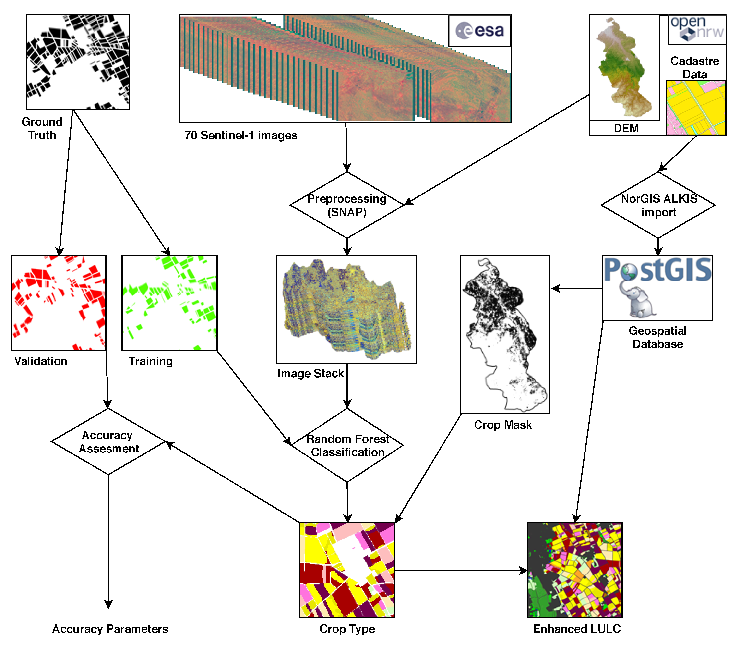
For preprocessing of remote sensing data, and SAR data in particular, using a digital elevation model (DEM) is advised [12]. In this study, we used the high-resolution, high-precision, openly available elevation data from open.NRW. The DEM is produced from LIDAR data with a point density of at least 4 points per m² and updated every six years. The final spatial resolution of 1 m has an absolute height error of less than 40 cm in most areas [44]. The newest version of the DEM can be found online [44], and a preprocessed version over the AOI of the DEM can be acquired via the TR32DB [45]. For compatibility reasons with the radar processing software Sentinel Application Platform ( SNAP) the DEM was projected to WGS84 and the spatial resolution reduced to 5 m [46].

For the delineation of the arable land, we exploited the real-estate register Amtliches Liegenschaftskataster-Informationssystem (ALKIS), which is freely available for the state Northrhinewestfalia (NRW) from Open.NRW [47]. ALKIS contains, in addition to other information, the usage of each of the 9 million property parcels in NRW. To identify the area of annually changing crops the agricultural parcels with the attribute “arable land” were selected. Based on the selection a crop/non-crop mask was calculated [48].

3. Methods

3.1. Preprocessing of the Sentinel-1 Radar Data Using the SNAP Toolbox

The preprocessed GRD images were individually processed using the SNAP Toolbox [49]. The following tools were executed on each acquisition:

• As a first step, a subset of the images was calculated by cropping the images to the extent of the AOI.
• To enhance the geometric accuracy, the precise orbit files were auto-downloaded from the ESA server and applied to the images. The precise orbit files are calculated within two weeks after the image acquisition and significantly enhance the geometric accuracy of the Sentinel-1 images.
• Next, the images were calibrated to beta0, which is the measured radar brightness [50], and a prerequisite for the next step.
• The highly accurate DEM from Open.NRW was used to perform a Radiometric Terrain Correction to gamma0. Thereby, based on the DEM, the terrain-induced radiometric effects are eliminated, and the signal is normalized for the local illuminated area [50].
• All SAR images inherit a salt-and-pepper-like noise [51]. A Gamma Map Speckle Filter with a 3 × 3 moving window was applied to reduce it.
• To project the images from slant range to ground range, a Range Doppler Terrain Correction was performed using the DEM from Open.NRW. [51]. Notably, a higher accuracy of the DEM translates into a higher horizontal accuracy of the projected image. The resampling of the preprocessed DEM to the image system was performed using Bicubic Interpolation. The calculation of the new image pixels in the final grid was done using nearest-neighbour resampling to avoid unnecessary mixing with neighbouring pixels. The final pixel spacing was set to 10 m and the reference system is UTM 32 N with WGS 84 as the reference ellipsoid.
• For better data handling, conversion of the raster values from linear to a decibel (dB) scale backscatter coefficient was applied.
• To reduce the amount of disc space being used for the images and to accelerate classification, the pixel-depth was reduced to unsigned integer with a linear scaling using slope and intercept of the histogram.

The graph to apply those steps in the SNAP software [52], and the final stacked image composite [53] can be downloaded via the TR32DB.

3.2. Supervised Random Forest Classification

The 70 individual Sentinel-1 images were stacked and a supervised pixel-based classification was performed using the independent training data from the mapping campaign. The Random Forest (RF) algorithm was used as the classifier, as it had already proved beneficial in other SAR-based crop classification scenarios [15,20,21]. The advantages of the RF classifier are its capabilities to handle high dimensional data and the ability to work without normally distributed data. While there are more advanced algorithms, such as the one developed by [22], previous studies have found the RF classifier to be highly accurate [54].

In the implementation of the RF classifier, 2000 pixel samples were randomly selected per class from all training fields. Next, those samples were randomly split for training and validating each tree. Two-thirds of the samples were used for training and one third for validation. The tuning parameters of the RF classifier left unchanged to the defaults of the R-package. This means that 500 trees with an unlimited node size built, and the variables tried at each split are set to the number of classes (eleven).

Validation of the gained classifications was conducted using the fields from the mapping campaign that had not been used for training the classifier. The resultant error matrix is the basis for the class specific accuracy measures, user’s accuracy, producer’s accuracy [55], and F1-Score [22]. For assessing the general accuracy of the classification, the overall accuracy [55] was calculated.

3.3. Real Estate Cadastre and Post-Classification Filtering

As can be seen in Figure 2, the raw ALKIS cadastre data downloaded from Open.NRW, were imported into a PostGIS database using the NorGIS software. Thereby, all different thematic geodata contained in the cadastre is available in QGIS. A selection of all agriculture parcels having agricultural as usage on the ALKIS cadastre data made it possible to acquire a crop/non-crop mask.

Only after that step is a post-classification filter reasonable. Otherwise, non-crop pixels would be considered in the filtering process, possibly degrading the classification quality. We used a majority filter with a circular (Von Neumann) neighbourhood, setting the center pixel to the majority value of the pixel values within the neighbourhood [56]. The filtering was conducted twice: the first one with a neighbourhood radius of three pixels, the second one with two pixels.

3.4. Open Source Software Used in this Study

One of the principles of the present study was to rely solely on Open Source Software. Preprocessing of the radar images was conducted using (SNAP) [49], which is developed by ESA and therefore, particularly suited to process ESA sensors, such as the Sentinel-1 used in this study. The actual multitemporal random forest classification was performed in R [57] (Version 3.4.3) using a freely available R-script [57] from [58] that uses the following R-packages: randomforest [59], Geospatial Data Abstraction Library (GDAL) [60], Raster [61], Maptools [62], and SP [63]. For postprocessing including the Error Matrix generation and the post classification filter, we used the Orfeo Toolbox [64], which provides a number of state-of-the-art remote sensing tools and has an active community. Map-making, integration of the ALKIS, cropping of the raster data, and preprocessing of the crop distribution maps was conducted in QGIS [65], one of the leading open-source GIS. The ALKIS data were imported to a PostGIS [66] geospatial database, which is based on PostgreSQL [67], using the free software ALKISimport [68]. The preprocessing of the DEM was achieved with GDAL [69].

4. Results

Using the proposed approach made it possible to classify 11 different crops with an accuracy of around 95%. The final crop classification map is presented in Figure 3. It covers the entire 2500 km² of the AOI at a spatial resolution of 10 m. It is available for download in the TR32DB [70].

As can be seen in

Table 4. Error Matrix of the proposed classification, shown in Figure 3.

		Validation (Ground Data)
		Pasture	Rape Seed	Potato	Maize	Sugar Beet	Barley	Wheat	Rye	Spring Barley	Pea	Carrot
Classification Data	Pasture	3093	0	0	0	0	116	0	0	25	3	0
	Rapeseed	6	11,045	0	0	0	3	0	0	0	0	0
	Potato	0	0	2845	0	0	0	0	0	0	0	0
	Maize	314	0	2	10,826	93	35	3	1	0	6	81
	Sugar Beet	32	0	1096	9	18,667	2	10	1	0	0	0
	Barley	49	0	0	0	0	27,979	3	247	7	0	0
	Wheat	40	0	0	0	0	4	14,345	2	0	0	0
	Rye	8	0	1	0	0	1228	2	5585	0	0	0
	Spring Barley	7	0	0	0	0	135	0	0	4855	0	0
	Pea	29	0	0	0	0	0	0	0	0	3105	0
	Carrot	0	0	0	0	0	1	0	0	0	0	2967

and

Table 5. Accuracy measures of the proposed classification, shown in Figure 3.

	User’s Accuracy	Producer’s Accuracy	F1-Score	Overall Accuracy
Pasture	96%	86%	91%	96.69%
Rapeseed	100%	100%	100%
Potato	100%	72%	84%
Maize	95%	100%	98%
Sugar Beet	94%	100%	97%
Barley	99%	95%	97%
Wheat	100%	100%	100%
Rye	82%	96%	88%
Spring Barley	97%	99%	98%
Pea	99%	100%	99%
Carrot	100%	97%	99%

, the accuracy of all crop classes was in the acceptable accuracy range, as all user and producer accuracy measures were beyond 80%, with one exception: −72% producer accuracy of the class potato, which was mixed up with sugar beet.

Integrating the external ALKIS data allowed crop areas to be focused on, as all non-crop areas were masked out. Thereby, applying the two times majority filter became feasible, which resulted in a 1.7% accuracy gain (Overall Accuracy: 96.69%). A map of the final classification is shown in Figure 3. Although 1.7% might not seem impressive, the advantages from this procedure go beyond the pure number. Most importantly, pixels values classified as a crop type and not within the feature class “agricultural land” of ALKIS are deleted, and the correct ALKIS land use class is assigned. Consequently, no agricultural land use is present in the final LULC map. However, if a map including the attributes of the ALKIS together with the crop type is needed, the creation of enhanced LULC maps, as demonstrated in Figure 4, is feasible.

To follow the principles of TOP, the workflow of the current study was designed and implemented with FOSS Figure 2. All of the necessary steps to perform the final crop classification could be successfully conducted in the following software environments:

• The Sentinel-1 images were pre-processed in SNAP [49].
• Transferring the ALKIS into a PostGIS database was performed with ALKISimport [68].
• Processing of the DEM from open.NRW was done in GDAL [69].
• Performing the random forest classification was executed in R [57].
• Post classification filtering and evaluating of the classification was achieved with the Orfeo Toolbox [64].
• Creating the final maps of the classification, as shown in Figure 3 and Figure 4 were conducted with QGIS [65].

5. Discussion

This paper presents an open-data and open-source remote sensing workflow to derive crop type for a region in west Germany, the area of the Rur Catchment. The all-weather capability of the used SAR sensor Sentinel-1 makes the results independent of the cloud coverage that is typical for the study region [14]. External data in the form of a height model and cadastre data [30] assisted the classification process. The final classification of 11 different crops shows a high accuracy of approx. 97% overall accuracy on a spatial resolution of 10 m.

A comparison with the LULC analysis based on optical data, shown in Figure 1, revealed merely 56% agreement of the two classifications within the agricultural area. As that dataset is available for download project internally [71], the differences could be further analyzed:

• 11% of the differences originate from incomplete disaggregation to the crop level in the optical classification. Merely superior classes such as agricultural field, or summer crop are given in the optical classification.
• Another 10% stems from the class rye, which is dissolved in the winter wheat class in the optical classification and correctly differentiated in the classification of this study.
• About 9% difference is due to roads and tracks that are modeled into the optical MDA classifications [14]. It is debatable whether that area is representative of the fields in the study area.

In addition to those shortcomings of the optical classification, the error matrix, shown in

Table 6. Error Matrix of the multi data approach (MDA) land use / land cover (LULC) classification with optical data shown in Figure 1 [71]. The classification was performed using the MDA described by [14], Overall Accuracy: 91.44%.

		Validation (Ground Data)									User’s Accuracy
		Rape Seed	Potato	Maize	Sugar Beet	Barley	Wheat	Summer Crops	Spring Barley	Pea
Classification Data	Rapeseed	2655	0	25	0	255	168	0	53	77	83%
	Potato	0	784	0	103	0	34	32	0	0	82%
	Maize	9	126	4582	70	95	0	279	0	2	89%
	Sugar Beet	0	79	538	11,265	7	2	118	0	35	94%
	Barley	0	30	21	1	6681	319	0	0	0	95%
	Wheat	3	51	11	26	120	13,311	0	8	21	98%
	Summer Crops	102	503	291	63	0	1	4062	13	116	79%
	Spring Barley	3	82	6	0	57	99	195	1076	20	70%
	Pea	0	0	0	0	0	0	9	0	988	99%
Producer’s Accuracy		96%	47%	84%	98%	93%	96%	87%	94%	78%

, reveals more confusion than the one from the current study shown in Table 4. Consequently, the overall accuracy is about 5% lower than that of the present study, although fewer classes were considered. Finally, the spatial resolution is increased from 15 m to 10 m, providing more details of the crop distribution. In summary, a superiority of the present study’s classification can be inferred in almost all aspects.

Another comparison was performed with the results of a recent study by [22]. He also used multitemporal Sentinel-1 images to distinguish similar crop types in another study region also situated in Germany. In general, the results of this study are consistent with the study by [22], who concluded that dense time series of SAR images provide a high crop-separation potential. The final crop classifications are not publicly available. Hence, the comparison had to be conducted with the accuracy numbers given in the publication.

Table 7. Comparison of the Producer’s Accuracy (PA) and User’s Accuracy (UA) (in %) of crop classes of the study carried out by [22] and of the present study. Unsatisfactory results below 80% are marked in red (80%–70%, 70%–60%, below 60%). The classes Oat, Pea, and Carrot, appeared merely in one of the classifications and were left out.

	Bargiel (2017) Season 1		Bargiel (2017) Season 2		Present Study
Crop	PA	UA	PA	UA	PA	UA
Pasture	96	89	96	92	86	96
Rapeseed	100	91	100	66	100	99.9
Potato	81	93	75	87	72	100
Maize	96	93	96	89	100	95
Sugar Beet	97	94	89	94	100	94
Barley	96	97	88	56	95	99
Wheat	90	97	88.2	98	100	100
Rye	93	93	89	74	96	82
Spring Barley	74	74	67	96	99	97
Mean	91.4	91.4	87.2	83.5	94.2	95.8

shows the direct comparison of the user and producer accuracies of both studies. The accuaries from [22] are taken from his most sophisticated crop classification, which uses information about the crop’s phenology. As can be seen, compared to the present study, there is a consistency on the high accuracy of pasture, maize, sugar beet, and wheat. Both studies revealed challenges to correctly classify potatoes, which is probably due to the alignment of the potato hills and various phenology due to varying planting dates [21]. The classes rye, and especially spring barley, was significantly better classified in the present study. This confusion could stem from fewer mapped fields and fewer Sentinel-1 images in the study by [22].

Although the current study’s results show less confusion, the algorithm of [22] seems more sophisticated, as it includes crop phenology information. However, it is not possible to compare the algorithms, the input data, or the obtained results as neither the source code nor the data is publicly shared.

That last aspect highlights the innovation of this study, which lies in the unique implementation of the workflow: All datasets used in the process, provided by ESA and open.NRW, are distributed as open data by the data providers, as well as in the TR32DB. Also, the ground reference of the study, about 1200 labeled agricultural fields, is shared. Furthermore, since the whole workflow is designed with FOSS, there are no additional costs for software and the source code is open. The combination of open data and FOSS allows reproducibility of the study, which enables other scientists to build upon this study’s results and evaluate their approaches with our data.

Next, crop-type classifications on larger scales are to be pursued and can be integrated into global agricultural systems [5]. In doing so, such systems can provide better outputs to enable the principles of agricultural intensification to be following, resulting in lower environmental impacts and higher food security.

However, upscaling the approach brings additional challenges. One is the availability and quality of external data. Geodata is often not available in such high precision as the geodata provided by open.NRW. For DEMs, that problem could be solved by relying on global data sets, such as the TanDEM-X derived DEM [72], which has recently been made freely available for scientific purposes in 90 m resolution. However, releasing the full resolution as open data would be favorable.

In the case of including external cadastre data into the classification process [30] or for post-classification fusion (compare Figure 4) a high spatial accuracy cannot be anticipated in many areas of the world. In such cases, ref. [73] present a smart way to improve the accuracy of external data, using a composite of multitemporal TerraSAR-X images as a spatial reference. As Sentinel-1 has a similarly high spatial accuracy [37], the approach could be adapted to areas where merely external geodata of lower spatial accuracy is available.

As shown above, the workflow’s implementation was performed in six different FOSS environments. Each environment has its characteristics, which involves a high demand of technical abilities necessary to execute the whole workflow. One way of coping with that issue is to create comprehensive documentation, user forums, and user mailing lists. It would also be possible to develop new software based on the environments used or to extend existing environments to meet the requirements of SAR-based crop classification in one environment.

6. Conclusions

This study demonstrates the feasibility of multitemporal microwave c-band SAR data from Sentinel-1 to distinguish crop types in our study site in western Germany. The final classification was evaluated with high accuracy, which was reached through the innovative integration of publicly available open data from Open.NRW. One of them was the high-resolution and high-precision DEM, which assisted the SAR preprocessing. The other one was the spatially highly accurate real estate register enabling to exclude the non- and special crop areas using the MDA. To overcome the problem of limited radar applications due to the complexity of radar data, all data used and produced in this study are openly available in the TR32DB. Additionally, the processing was done solely with FOSS. Consequently, all the results are reproducible without any additional data or software costs. Hence, the current study makes a substantial contribution to science in the context of microwave-based crop classification.

References

1. FAO; IFAD; UNICEF; WHO. The State of Food Security and Nutrition in the World 2017: Building Resilience for Peace and Food Security; FAO: Rome, Italy, 2017. [Google Scholar]
2. FAO. The Future of Food and Agriculture. Trends and Challenges; FAO Rome: Rome, Italy, 2017. [Google Scholar]
3. Godfray, H.C.J.; Garnett, T. Food security and sustainable intensification. Philo. Trans. R. Soc. B 2014, 369, 20120273. [Google Scholar] [CrossRef]
4. Atzberger, C. Advances in remote sensing of agriculture: Context description, existing operational monitoring systems and major information needs. Remote Sens. 2013, 5, 949–981. [Google Scholar] [CrossRef] [Green Version]
5. Fritz, S.; See, L.; Bayas, J.C.L.; Waldner, F.; Jacques, D.; Becker-Reshef, I.; Whitcraft, A.; Baruth, B.; Bonifacio, R.; Crutchfield, J.; et al. A comparison of global agricultural monitoring systems and current gaps. Agric. Syst. 2018. [Google Scholar] [CrossRef]
6. Bareth, G. GIS-and RS-based spatial decision support: Structure of a spatial environmental information system (SEIS). Int. J. Digit. Earth 2009, 2, 134–154. [Google Scholar] [CrossRef]
7. Machwitz, M.; Hass, E.; Junk, J.; Udelhoven, T.; Schlerf, M. CropGIS–A web application for the spatial and temporal visualization of past, present and future crop biomass development. Comput. Electron. Agric. 2018. [Google Scholar] [CrossRef]
8. Xiong, J.; Thenkabail, P.S.; Gumma, M.K.; Teluguntla, P.; Poehnelt, J.; Congalton, R.G.; Yadav, K.; Thau, D. Automated cropland mapping of continental Africa using Google Earth Engine cloud computing. ISPRS J. Photogramm. Remote Sens. 2017, 126, 225–244. [Google Scholar] [CrossRef] [Green Version]
9. Kersebaum, K.C.; Hecker, J.M.; Mirschel, W.; Wegehenkel, M. Modelling water and nutrient dynamics in soil–crop systems: A comparison of simulation models applied on common data sets. In Modelling Water and Nutrient Dynamics in Soil–Crop Systems; Springer: New York, NY, USA, 2007; pp. 1–17. [Google Scholar] [CrossRef]
10. Anderson, J.R. A Land Use and Land cover Classification System for Use with Remote Sensor Data; US Government Printing Office: Washington, DC, USA, 1976; Volume 964.
11. Xie, Y.; Sha, Z.; Yu, M. Remote sensing imagery in vegetation mapping: A review. J. Plant Ecol. 2008, 1, 9–23. [Google Scholar] [CrossRef]
12. Jensen, J.R. Remote Sensing of the Environment: An Earth Resource Perspective 2/e; Pearson Education: New Delhi, India, 2009. [Google Scholar]
13. Vuolo, F.; Neuwirth, M.; Immitzer, M.; Atzberger, C.; Ng, W.T. How much does multi-temporal Sentinel-2 data improve crop type classification? Int. J. Appl. Earth Obs. Geoinf. 2018, 72, 122–130. [Google Scholar] [CrossRef]
14. Waldhoff, G.; Lussem, U.; Bareth, G. Multi-Data Approach for remote sensing-based regional crop rotation mapping: A case study for the Rur catchment, Germany. Int. J. Appl. Earth Obs. Geoinf. 2017, 61, 55–69. [Google Scholar] [CrossRef]
15. Sonobe, R.; Tani, H.; Wang, X.; Kobayashi, N.; Shimamura, H. Random forest classification of crop type using multi-temporal TerraSAR-X dual-polarimetric data. Remote Sens. Lett. 2014, 5, 157–164. [Google Scholar] [CrossRef] [Green Version]
16. Heupel, K.; Spengler, D.; Itzerott, S. A Progressive Crop-Type Classification Using Multitemporal Remote Sensing Data and Phenological Information. PFG- Photogramm. Remote Sens. Geoinf. Sci. 2018, 86, 1–17. [Google Scholar] [CrossRef] [Green Version]
17. McNairn, H.; Shang, J. A review of multitemporal synthetic aperture radar (SAR) for crop monitoring. In Multitemporal Remote Sensing; Springer: New York, NY, USA, 2016; pp. 317–340. [Google Scholar] [CrossRef]
18. Kenduiywo, B.K.; Bargiel, D.; Soergel, U. Crop-type mapping from a sequence of Sentinel 1 images. Int. J. Remote Sens. 2018, 1–22. [Google Scholar] [CrossRef]
19. Whitcraft, A.K.; Vermote, E.F.; Becker-Reshef, I.; Justice, C.O. Cloud cover throughout the agricultural growing season: Impacts on passive optical earth observations. Remote Sens. Environ. 2015, 156, 438–447. [Google Scholar] [CrossRef]
20. Hütt, C.; Koppe, W.; Miao, Y.; Bareth, G. Best Accuracy Land Use/Land Cover (LULC) Classification to Derive Crop Types Using Multitemporal, Multisensor, and Multi-Polarization SAR Satellite Images. Remote Sens. 2016, 8, 684. [Google Scholar] [CrossRef] [Green Version]
21. Hütt, C.; Waldhoff, G. Multi-data approach for crop classification using multitemporal, dual-polarimetric TerraSAR-X data, and official geodata. Eur. J. Remote Sens. 2018, 51, 62–74. [Google Scholar] [CrossRef]
22. Bargiel, D. A new method for crop classification combining time series of radar images and crop phenology information. Remote Sens. Environ. 2017, 198, 369–383. [Google Scholar] [CrossRef]
23. Whelen, T.; Siqueira, P. Time-series classification of Sentinel-1 agricultural data over North Dakota. Remote Sens. Lett. 2018, 9, 411–420. [Google Scholar] [CrossRef]
24. Schmullius, C.; Thiel, C.; Pathe, C.; Santoro, M. Radar time series for land cover and forest mapping. In Remote Sensing Time Series; Springer: New York, NY, USA, 2015; pp. 323–356. [Google Scholar] [CrossRef]
25. Nosek, B.A.; Alter, G.; Banks, G.C.; Borsboom, D.; Bowman, S.D.; Breckler, S.J.; Buck, S.; Chambers, C.D.; Chin, G.; Christensen, G.; et al. Promoting an open research culture. Science 2015, 348, 1422–1425. [Google Scholar] [CrossRef] [Green Version]
26. McNutt, M. Taking up TOP. Science 2016, 352. [Google Scholar] [CrossRef] [Green Version]
27. Steiniger, S.; Hunter, A.J. The 2012 free and open source GIS software map–A guide to facilitate research, development, and adoption. Comput. Environ. Urban Syst. 2013, 39, 136–150. [Google Scholar] [CrossRef]
28. Rocchini, D.; Petras, V.; Petrasova, A.; Horning, N.; Furtkevicova, L.; Neteler, M.; Leutner, B.; Wegmann, M. Open data and open source for remote sensing training in ecology. Ecol. Inform. 2017, 40, 57–61. [Google Scholar] [CrossRef]
29. Bareth, G. Multi-Data Approach (MDA) for enhanced land use and land cover mapping. Int. Arch. Photogramm. Remote Sens. Spat. Inf. Sci. Part B 2008, 8, 1059–1066. [Google Scholar]
30. Waldhoff, G.; Eichfuss, S.; Bareth, G. Integration of remote sensing data and basic geodata at different scale levels for improved land use analyses. Int. Arch. Photogramm. Remote Sens. Spat. Inf. Sci. 2015, 40, 85. [Google Scholar] [CrossRef] [Green Version]
31. Curdt, C.; Hoffmeister, D. Research data management services for a multidisciplinary, collaborative research project: Design and implementation of the TR32DB project database. Program 2015, 49, 494–512. [Google Scholar] [CrossRef]
32. Woodcock, C.E.; Allen, R.; Anderson, M.; Belward, A.; Bindschadler, R.; Cohen, W.; Gao, F.; Goward, S.N.; Helder, D.; Helmer, E.; et al. Free access to Landsat imagery. Science 2008, 320, 1011. [Google Scholar] [CrossRef] [PubMed]
33. Wulder, M.A.; Masek, J.G.; Cohen, W.B.; Loveland, T.R.; Woodcock, C.E. Opening the archive: How free data has enabled the science and monitoring promise of Landsat. Remote Sens. Environ. 2012, 122, 2–10. [Google Scholar] [CrossRef]
34. Wulder, M.A.; Coops, N.C. Make Earth observations open access: Freely available satellite imagery will improve science and environmental-monitoring products. Nature 2014, 513, 30–32. [Google Scholar] [CrossRef]
35. ESA. Free Access to Copernicus Sentinel Satellite Data. 2013. Available online: http://www.esa.int/Our_Activities/Observing_the_Earth/Copernicus/Free_access_to_Copernicus_Sentinel_satellite_data/ (accessed on 20 February 2020).
36. Torres, R.; Snoeij, P.; Geudtner, D.; Bibby, D.; Davidson, M.; Attema, E.; Potin, P.; Rommen, B.; Floury, N.; Brown, M.; et al. GMES Sentinel-1 mission. Remote Sens. Environ. 2012, 120, 9–24. [Google Scholar] [CrossRef]
37. Schubert, A.; Small, D.; Miranda, N.; Geudtner, D.; Meier, E. Sentinel-1A product geolocation accuracy: Commissioning phase results. Remote Sens. 2015, 7, 9431–9449. [Google Scholar] [CrossRef] [Green Version]
38. Copernicus. Sentinel-1a IW GRDH Images from Orbit 37, Growing Season 2017. CRC/TR32 Database (TR32DB). 2018. Available online: http://www.tr32db.uni-koeln.de/data.php?dataID=1846 (accessed on 20 February 2020).
39. Copernicus. Sentinel-1b IW GRDH Images from Orbit 37, Growing Season 2017. CRC/TR32 Database (TR32DB). 2018. Available online: http://www.tr32db.uni-koeln.de/data.php?dataID=1847 (accessed on 20 February 2020).
40. Copernicus. Sentinel-1a IW GRDH Images from Orbit 88, Growing Season 2017. CRC/TR32 Database (TR32DB). 2018. Available online: http://www.tr32db.uni-koeln.de/data.php?dataID=1848 (accessed on 20 February 2020).
41. Copernicus. Sentinel-1b IW GRDH Images from Orbit 88, Growing Season 2017. CRC/TR32 Database (TR32DB). 2018. Available online: http://www.tr32db.uni-koeln.de/data.php?dataID=1849 (accessed on 20 February 2020).
42. Waldhoff, G.; Herbrecht, M. Crop Type Distribution Mapping 2017. CRC/TR32 Database (TR32DB). 2018. Available online: http://www.tr32db.uni-koeln.de/data.php?dataID=1820 (accessed on 20 February 2020).
43. Hütt, C. Training and Validation Data for a Crop Type Classification of the TR32-2017—Based on the Crop Type Distribution Mapping 2017. CRC/TR32 Database (TR32DB). 2018. Available online: http://www.tr32db.uni-koeln.de/data.php?dataID=1818 (accessed on 20 February 2020).
44. Bezirksregierung Köln. Digitales Geländemodell (DGM). 2018. Available online: https://www.bezreg-koeln.nrw.de/brk_internet/geobasis/hoehenmodelle/gelaendemodell/index.html (accessed on 20 February 2020).
45. Bezirksregierung Köln. Digital Elevation Model (DGM1) of the Rur Catchment, Based on Data from Bezirksregierung Köln, Bonn, Germany. CRC/TR32 Database (TR32DB). 2017. Available online: http://www.tr32db.uni-koeln.de/data.php?dataID=1690 (accessed on 20 February 2020).
46. Hütt, C. DGM1, WGS84, 5m, Based on Data from Bezirksregierung Köln, Bonn, Germany. CRC/TR32 Database (TR32DB). 2018. Available online: http://www.tr32db.uni-koeln.de/data.php?dataID=1851 (accessed on 20 February 2020). [CrossRef]
47. Bezirksregierung Köln. Liegenschaftskataster. 2018. Available online: https://www.bezreg-koeln.nrw.de/brk_internet/geobasis/liegenschaftskataster/index.html (accessed on 20 February 2020).
48. Hütt, C. Crop Mask 2017 Derived from the ALKIS. CRC/TR32 Database (TR32DB). 2018. Available online: http://www.tr32db.uni-koeln.de/data.php?dataID=1850 (accessed on 20 February 2020). [CrossRef]
49. SNAP-ESA. Sentinel Application Platform v 5.0.1. 2017. Available online: http://step.esa.int/main/download/snap-download/ (accessed on 20 February 2020).
50. Small, D. Flattening gamma: Radiometric terrain correction for SAR imagery. IEEE Trans. Geosci. Remote Sens. 2011, 49, 3081–3093. [Google Scholar] [CrossRef]
51. Curlander, J.; McDonough, R. Synthetic Aperture Radar: Systems and Signal Processing; JohnWiley& Sons: New York, NY, USA, 1991. [Google Scholar]
52. Hütt, C. Enhanced Graph File for Processing Sentinel-1 Images using SNAP. CRC/TR32 Database (TR32DB). 2018. Available online: http://www.tr32db.uni-koeln.de/data.php?dataID=1803 (accessed on 20 February 2020). [CrossRef]
53. Hütt, C. Sentinel-1 Composite of the Growing Season 2017. CRC/TR32 Database (TR32DB). 2018. Available online: http://www.tr32db.uni-koeln.de/data.php?dataID=1845 (accessed on 20 February 2020). [CrossRef]
54. Rodriguez-Galiano, V.F.; Ghimire, B.; Rogan, J.; Chica-Olmo, M.; Rigol-Sanchez, J.P. An assessment of the effectiveness of a random forest classifier for land-cover classification. ISPRS J. Photogramm. Remote Sens. 2012, 67, 93–104. [Google Scholar] [CrossRef]
55. Congalton, R.G.; Green, K. Assessing the Accuracy of Remotely Sensed Data: Principles and Practices; CRC Press, Taylor &Francis: Boca Raton, FL, USA, 2008. [Google Scholar]
56. Orfeo Developement Team. Classification Map Regularization. 2018. Available online: https://www.orfeo-toolbox.org/CookBook/Applications/app_ClassificationMapRegularization.html (accessed on 20 February 2020).
57. R Core Team. R: A Language and Environment for Statistical Computing. 2018. Available online: https://www.R-project.org/ (accessed on 20 February 2020).
58. Horning, N. RandomForestClassification. 2013. Available online: https://bitbucket.org/rsbiodiv/randomforestclassification/commits/534bc2f (accessed on 20 February 2020).
59. Liaw, A.; Wiener, M. Classification and Regression by randomForest. R News 2002, 2, 18–22. [Google Scholar]
60. Bivand, R.; Keitt, T.; Rowlingson, B. Rgdal: Bindings for the ’Geospatial’ Data Abstraction Library; R package version 1.2-15. 2017. Available online: https://CRAN.R-project.org/package=rgdal (accessed on 20 February 2020).
61. Hijmans, R.J. Raster: Geographic Data Analysis and Modeling; R package version 2.6-7. 2017. Available online: https://CRAN.R-project.org/package=raster (accessed on 20 February 2020).
62. Bivand, R.; Lewin-Koh, N. Maptools: Tools for Reading and Handling Spatial Objects; R package version 0.9-2. 2017. Available online: https://CRAN.R-project.org/package=maptools (accessed on 20 February 2020).
63. Pebesma, E.J.; Bivand, R.S. Classes and methods for spatial data in R. R News 2005, 5, 9–13. [Google Scholar]
64. Orfeo Developement Team. Orfeo Toolbox V. 5.8.0. 2017. Available online: https://www.orfeo-toolbox.org (accessed on 20 February 2020).
65. QGIS Development Team. Open Source Geospatial Foundation Project. 2017. Available online: http://qgis.org (accessed on 20 February 2020).
66. PostGIS. Spatial and Geographic Objects for PostgreSQL 2.4.3. 2017. Available online: https://postgis.net (accessed on 20 February 2020).
67. PostgreSQL. The World’s Most Advanced Open Source Relational Database 10.2. 2017. Available online: https://www.postgresql.org/ (accessed on 20 February 2020).
68. NorGIS. ALKIS Import. 2017. Available online: https://github.com/norBIT/alkisimport (accessed on 20 February 2020).
69. GDAL Development Team. GDAL—Geospatial Data Abstraction Library; Version 2.2.3. 2017. Available online: http://www.gdal.org (accessed on 20 February 2020).
70. Hütt, C. Crop Classification 2017 of the Rur Catchement Using Sentinel-1 and Data from open.NRW. CRC/TR32 Database (TR32DB). 2018. Available online: http://www.tr32db.uni-koeln.de/data.php?dataID=1844 (accessed on 20 February 2020). [CrossRef]
71. Waldhoff, G.; Herbrecht, M. Enhanced land Use Classification of 2017 for the Rur Catchment. CRC/TR32 Database (TR32DB). 2018. Available online: http://www.tr32db.uni-koeln.de/data.php?dataID=1795 (accessed on 20 February 2020). [CrossRef]
72. Zink, M.; Bachmann, M.; Brautigam, B.; Fritz, T.; Hajnsek, I.; Moreira, A.; Wessel, B.; Krieger, G. TanDEM-X: The new global DEM takes shape. IEEE Geosci. Remote Sens. Mag. 2014, 2, 8–23. [Google Scholar] [CrossRef]
73. Zhao, Q.; Hütt, C.; Lenz-Wiedemann, V.I.; Miao, Y.; Yuan, F.; Zhang, F.; Bareth, G. Georeferencing multi-source geospatial data using multi-temporal TerraSAR-X imagery: A case study in Qixing Farm, northeast China. Photogrammetrie-Fernerkundung-Geoinformation 2015, 2015, 173–185. [Google Scholar] [CrossRef]
Figure 1. Location of the study region Rur Catchment and land use / land cover (LULC) analysis of 2017 using the Multi Data Approach (MDA) [14] with optical satellite data and external data. Screenshot from the online available WebGIS of the TR32 project database (TR32DB).
Ijgi 09 00120 g001
Figure 2. Flowchart of the data flows and processing steps of this work.
Ijgi 09 00120 g002
Figure 3. Final Classification with a two times post classification majority filter of the whole area of interest (AOI) covering about 2500 km2.
Ijgi 09 00120 g003
Figure 4. Enhanced land use/land cover (LULC) map by fusing the Sentinel-1 based Crop Classification with generalized ATKIS cadastre data.
Ijgi 09 00120 g004