Using Areal Interpolation to Deal with Differing Regional Structures in International Research


1
Department of Social Geography and Regional Development, Faculty of Science, Charles University, Albertov 6, 128 43 Prague 2, Czechia
2
Department of Geography, Faculty of Education, Catholic University in Ruzomberok, Hrabovska cesta 1, 034 01 Ruzomberok, Slovakia
*
Author to whom correspondence should be addressed.
ISPRS Int. J. Geo-Inf. 2020, 9(2), 126; https://0-doi-org.brum.beds.ac.uk/10.3390/ijgi9020126
Submission received: 14 January 2020
/
Revised: 11 February 2020
/
Accepted: 20 February 2020
/
Published: 22 February 2020
Abstract
:When working with regional data from different countries, issues concerning data comparability need to be solved, including regional comparability. Differing regional unit size is a common issue which influences the results of socio-economic analyses. In this paper, we introduce a strategy to deal with the regional incomparability of administrative data in international research. We propose a methodological approach based on the areal interpolation method, which facilitates the usage of advanced spatial analyses. To illustrate, we analyze spatial patterns of unemployment in seven Central European countries. We use a very detailed spatial (municipal) level to reveal local tendencies. To have comparable units across the whole region, we apply the areal interpolation method, a process of projecting data from source administrative units to the target structure of a grid. After choosing the most suitable grid structure and projecting the data onto the grid, we perform a hot spot analysis to show the benefits of the grid structure for socio-economic analyses. The proposed approach has great potential in international research for its methodological correctness and the ability to interpret results.
1. Introduction
We live in an era of open and big data. Spatial micro-level and individual data are available for researchers across disciplines. In the case of statistical regional data, human geographers and regional scientists usually want to work with the most detailed units available, such as ZIP codes or municipalities. These data enable us to identify local specifics, which may be hidden when working with larger regional units. However, it is uncommon to find micro-regional international analyses using such detailed data. Although governments invest a lot of money in the harmonization of country-specific data, the availability of comparable data is still problematic. It can be documented in the example of cross-national comparative research [1] or spatial data infrastructure [2].
Even if data is available, one has to be careful when using spatially detailed data. Specific adjustments are often needed before performing statistical and spatial analyses. In general, regional and local spatial data infrastructures have been developing faster than national and global ones, because of “more complex procedures for data harmonizing which comes from many sources with different standards and included a big number of actors” ([2], p. 62). Thus, it is no surprise that there is a lack of international analyses on the regional micro-level due to low data availability and comparability.
When undertaking empirical analyses using data from multiple countries, there are several methodological issues. Three aspects of data comparability affect the analyses: the subject (definitions, different laws, census vs. samples), time (timing of collection of data, periodicity), and space/region (spatial delimitation of units with different shapes and average sizes). Varying regional structures in different countries is the third issue we would like to address. Differing unit sizes may impede the analysis and skew results. In Europe, the statistical office EUROSTAT makes efforts to have comparable data from all member countries through standardized regional delimitation. While EUROSTAT has been partly successful in introducing standardized units on a higher level (NUTS 2), lower regional levels are still very different across European countries.
The main goal of this paper is to introduce a strategy on how to deal with the regional comparability issue, which is one of many issues connected with data comparability. Differences among national systems impede the analyses and influence the interpretation of results, which needs to reflect the national context [3]. Working with uniform, regional structure instead of different administrative systems is the solution to the regional comparability issue. It may facilitate the usage and interpretation of advanced spatial analyses in international research. Thus, the area-area spatial data transformation should be applied [4]. We propose a methodological approach based on areal interpolation as the most convenient method to achieve the main goal. We specifically ask the following questions: what are the main advantages of this approach? Are its strengths greater than its shortcomings? What are the possible biases?
Usually, areal interpolation is used for recalculation from a source structure to a given, pre-defined target structure [5]. We use this method in a slightly different way, to homogenize regional units in different countries to a standardized spatial structure. This homogenization is methodologically more precise for subsequent spatial analyses and statistics based on spatial weighting schemes. Moreover, it helps us to interpret results more accurately. We express this with the example of spatial autocorrelation (hot spot analysis), which helps to reveal spatial patterns. Yet, for better data comparability across different systems (such as countries) or across time at different geographical levels [6], it would be best to work with a regular grid. To do this, we first have to recalculate the values from source units to this regular grid. This paper considers and tests two different areal interpolation methods for these purposes, (i) simple area weighting and (ii) areal kriging.
We showcase this methodology on unemployment in an area of Central Europe consisting of seven countries (Austria, Czechia, Germany, Hungary, Poland, Slovakia, and Slovenia). Comparability issues are particularly visible here, especially when you compare the very fragmented regional structure in Czechia (more than 6,000 municipalities, 12 square kilometres on average) and Poland (less than 2,500 municipalities with an average of more than 120 square kilometres). Besides regional structure size differences in respective countries, the differences between municipality sizes within these countries are enormous. For example, Prague has an area of 496 square kilometres which is more than 30 times larger than the average Czech municipality. As a testing dataset, we used unemployment data from 2010, which are available on a municipal level at statistical offices in respective countries.
2. Spatial Data Transformation through Areal Interpolation
The issue of spatial data transformation between two different systems of spatial units is traditionally a challenging topic in geospatial literature [4,7,8]. In geostatistics, spatial data transformation is often referred to as the change of support problem (COSP) [5,7]. Depending on the type of source and target spatial data (point, line, area, surface), we can distinguish between many COSPs using different spatial interpolation techniques. For our purposes, we use the areal interpolation method and area-area COSP. For a detailed description and review of COSP and spatial interpolation techniques, see [4,7].
Areal interpolation (or cross-area estimation) enables us to recalculate values from one polygonal delimitation to another. It is understood as “a set of methods that can estimate an aggregate attribute of one areal unit system based on that of another, spatially incongruent, system in which the attribute data were collected” ([9], p. 645). In general, areal interpolation is the transformation of data from one set of polygons to another, i.e., from source regional structure to target regional structure. It allows us to change the scale, i.e., to downscale or upscale the regional level of data under study. Thus, we can predict the phenomena in census tracts from municipality data and vice versa. Many interpolation methods and techniques with varying data and assumption requirements have been developed [10]. The two basic approaches are cartographic and geostatistical (surface-oriented) methods [5].
Cartographic approaches of areal interpolation are based on weighting by the area of overlap between the source (municipalities) and the target (grid cells) units [5]. We use the simplest form, the simple areal weighting method. In this method, the sizes of the source and target zones are used to weight the source zone values which preserves the volume of the original population. One limitation of this simple method is that homogenous uniform distribution of population within each source zone (municipality) is assumed [9,11] which is rarely true in geographical reality. However, this is not an issue in our case since we aim to detect overall spatial patterns, not to make precise micro-scale estimations. Other more advanced techniques deal with the more realistic expectation that source zones are heterogeneous but have an unknown structure [12].
Geostatistical methods generate surface and are often referred to as surface-oriented [5]. We use a geostatistical interpolation technique that extends kriging theory to data aggregated over polygons such as discrete counts. This technique differs from standard geostatistical interpolation methods which do not take the polygon sizes into account and work with point data or centroids as representatives of polygonal data. In areal interpolation based on the kriging disaggregation technique [13], reaggregating polygonal data from municipalities to a regular grid is a two-step process. First, a smooth prediction surface is created from data for a source regional structure, municipalities in our case. Because of the nature of our data, which is measured in municipalities over a specific period, we use an areal interpolation for event counts. This technique produces a surface that predicts the underlying chance of detecting a person (15–64 years old, unemployed in our case) at a specific location. The predicted surface can be interpreted as a density map. To build a valid model and find the surface with the lowest standard error, we used interactive variography. Second, the prediction surface is aggregated back to the new set of polygons. Overdispersed Poisson areal interpolation enables the ability to predict the number of counts for each specified square in a regular grid.
For our purposes, we apply and compare two areal interpolation methods, simple area weighting and areal kriging. Before we can use either method, it is necessary to choose a target regional structure. We decided to create a regular grid structure which can be found in many population studies [14,15]. We did so across the whole study area to harmonize municipal size differences in the respective countries. We use the best grid based on the goodness of fit statistic. It is important to emphasise that this is not up-scaling nor down-scaling, but homogenization. As a result, we can still work with sufficient spatial detail. Overdispersed Poisson areal interpolation allows us to predict the number of counts for each specified square on a regular grid.
Every COSP, including areal interpolation, generates transformation error. The potential error of areal interpolation can be estimated by two measures defined by Simpson [16]: the degree of hierarchy and the degree of fit. These measures express the amount of estimation involved in the data transformation process from one spatial system to another. The degree of hierarchy for the entire study area is equal to the proportion of all source zones (municipalities) that fall completely within any of the target zones (grids) [8,16]. It gives evidence of nesting. The degree of hierarchy [16] is calculated as:
where i = a source spatial unit (municipality), j = a target spatial unit (grid cell), wij = the proportion of the municipality that overlaps the grid cell, and n = the number of source units (municipalities). The degree of fit for the entire study area is the proportion of sums of the maximal weight of each source unit (municipality) and the number of all source units (municipalities) [8,16]. It measures the extent of overlap between two spatial systems. This measure is more accurate because it recognises that municipality boundaries may be close to the grid cell boundaries even when they do not fit them exactly. The degree of fit [16] is calculated as:
where max wij is the maximum proportion of the municipality i to grid j overlap. As other researchers dealing with areal interpolation [8,17], we also use these two Simpson’s measures to estimate the ‘goodness of fit’ between the real regional structure and the regular structures with different grid sizes.
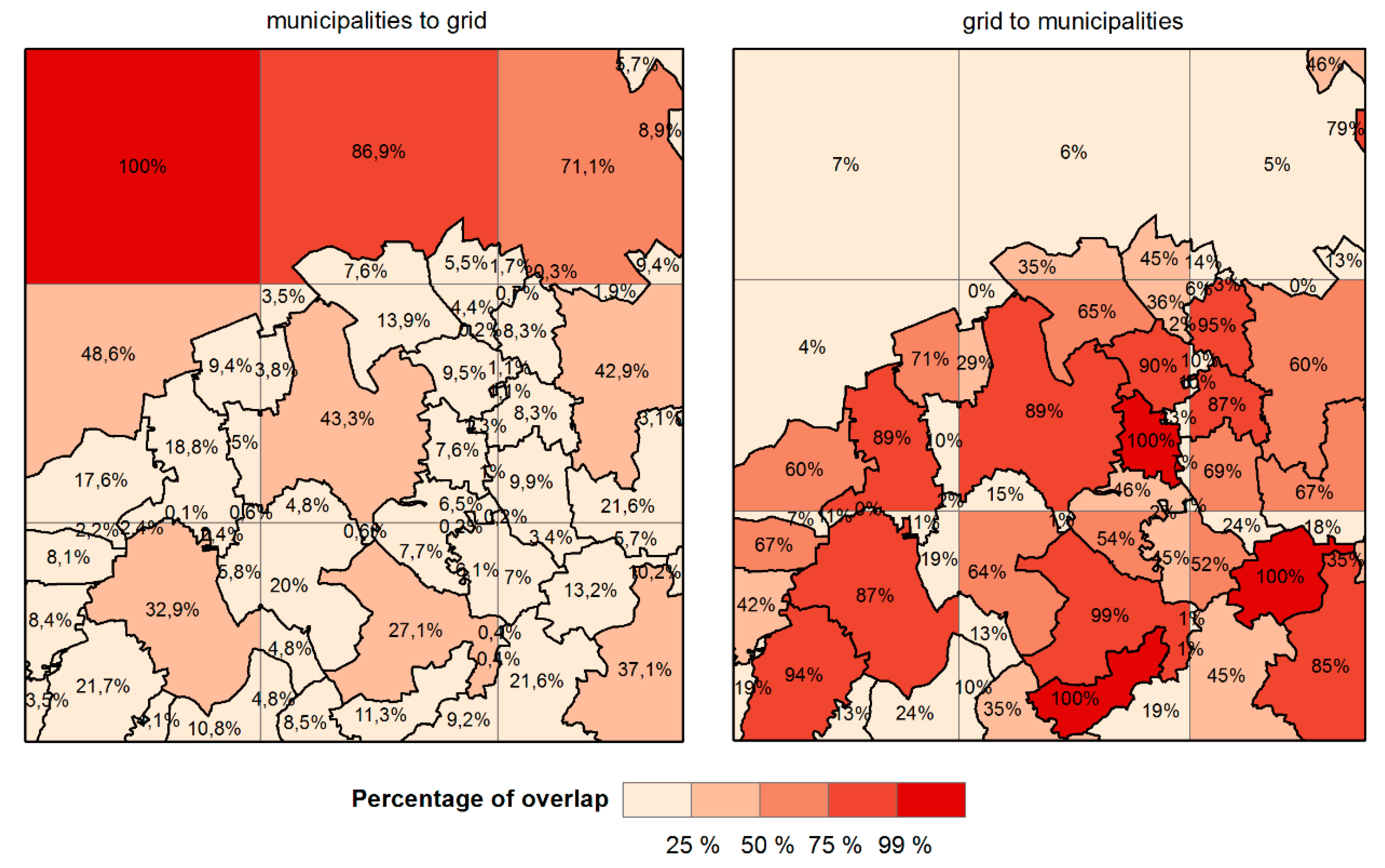
These goodness of fit statistics were used to choose the best fit target grid structure. First, we assessed the overlap between municipalities and the grid structure for different sizes of the grid cells. We take into account both directions of these degrees: municipalities-to-grid (how the municipalities fit into the grid) and grid-to-municipalities (how the grid fits the municipal structure). The difference between calculations of the percentage of overlay for the degree of fit is best documented by visualization in Figure 1. Usually, only one direction is used. In our use case, it is important to have the maximum possible balance between these two directions. Since we search for the best-fit solution and do not have a given target structure, we use the degree of fit as a “two-way fit”.
3. Central European Region as a Case Study
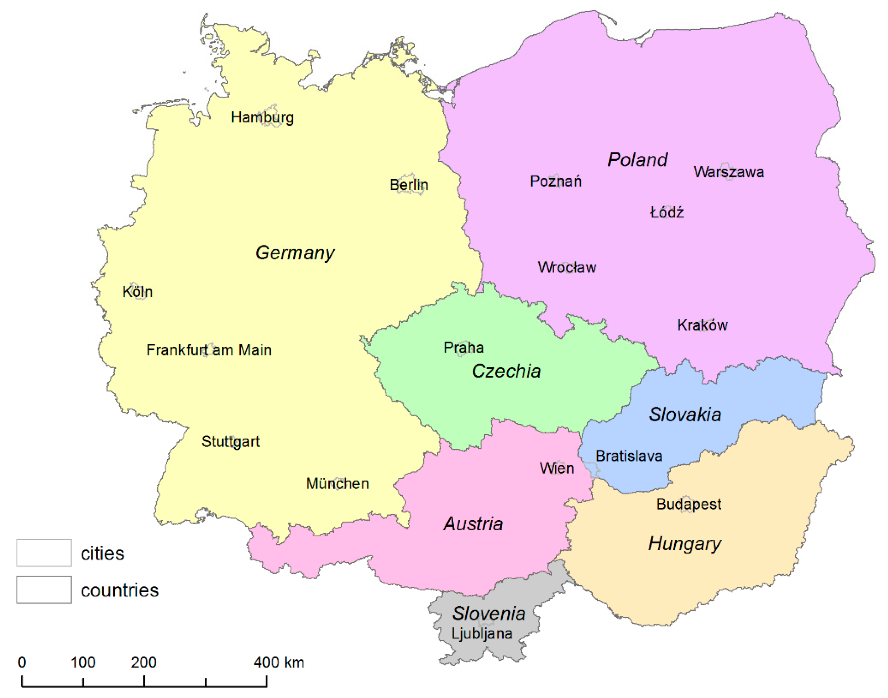
The Central European Region (CER) serves as a case study region for testing our strategy to deal with empirical data. We collected comparable unemployment data available on a very detailed spatial (municipal) level in a relatively big, international geographical area. The study area consists of seven Central European countries: Austria, Czechia, Germany, Hungary, Poland, Slovakia, and Slovenia. These seven countries met our requirements and created a large study area suitable for our methodological aims—it is a compact area with many different regional structures (municipality sizes). It also has the potential for subsequent empirical analyses because of significant spatial patterns of unemployment. We are aware of the problematic perception and delimitation of Central Europe [18], but we use the term Central European Region (CER) throughout the paper. The CER is depicted in Figure 2.
While analysing areal data, one has to face the Modifiable Area Unit Problem (MAUP). The MAUP arises whenever we work with spatially aggregated data, no matter the scientific discipline. This well-known problem shows the sensitivity of results to the arbitrary choice of spatial aggregation units where analyses are made [19,20]. The results are possibly biased when a less fragmented (thus more aggregated) regional structure is used [21,22].
By choosing different delimitation or zoning, one can obtain very different or even contradictory results. The interpretation of results is thus affected by the selected regional structure used. To mitigate the MAUP problem, one can use the most detailed data available, as we did here. In this case, it is municipalities (LAU2—Local administrative units in the European Union). However, there are huge differences in regional structures in the respective countries, see Table 1.
Another problem is data. First, many socio-economic characteristics are not available at such a detailed level. Second, the definition of a characteristic often differs in respective countries, and this issue of data comparability should be solved. Unemployment rate was chosen as one of the few economic characteristics available on the necessary detailed spatial level. Since the unemployment rate is defined slightly differently in each country, we have settled for a common definition. The unemployment rate as we define it in this paper is the share of unemployed persons (job seekers) within the population aged 15–64. We use data from 2010 (unemployed in October 2010 and population on 31 December 2010) gained from official statistical sources in the studied countries. It is necessary to bear in mind that due to the different definition of unemployment used in this paper, results are not comparable to official published statistics and are lower than the rates found elsewhere. For descriptive statistics of unemployment in the studied countries, see Table 2.
Even when the most suitable data has been selected, the issue of relatively incomparable regional structures remains unresolved. Thus, we apply the areal interpolation method. This converts differing regional structures in studied countries into a single regular grid structure for the whole studied area. However, we still have to choose the best specific grid size; we do this using goodness of fit statistics. First, we assessed the overlap between municipalities and the grid structure for different sizes of the grid cells. We take both directions of these degrees into account: municipalities-to-grid (how the municipalities fit into the grid) and grid-to-municipalities (how the grid fits the municipal structure).
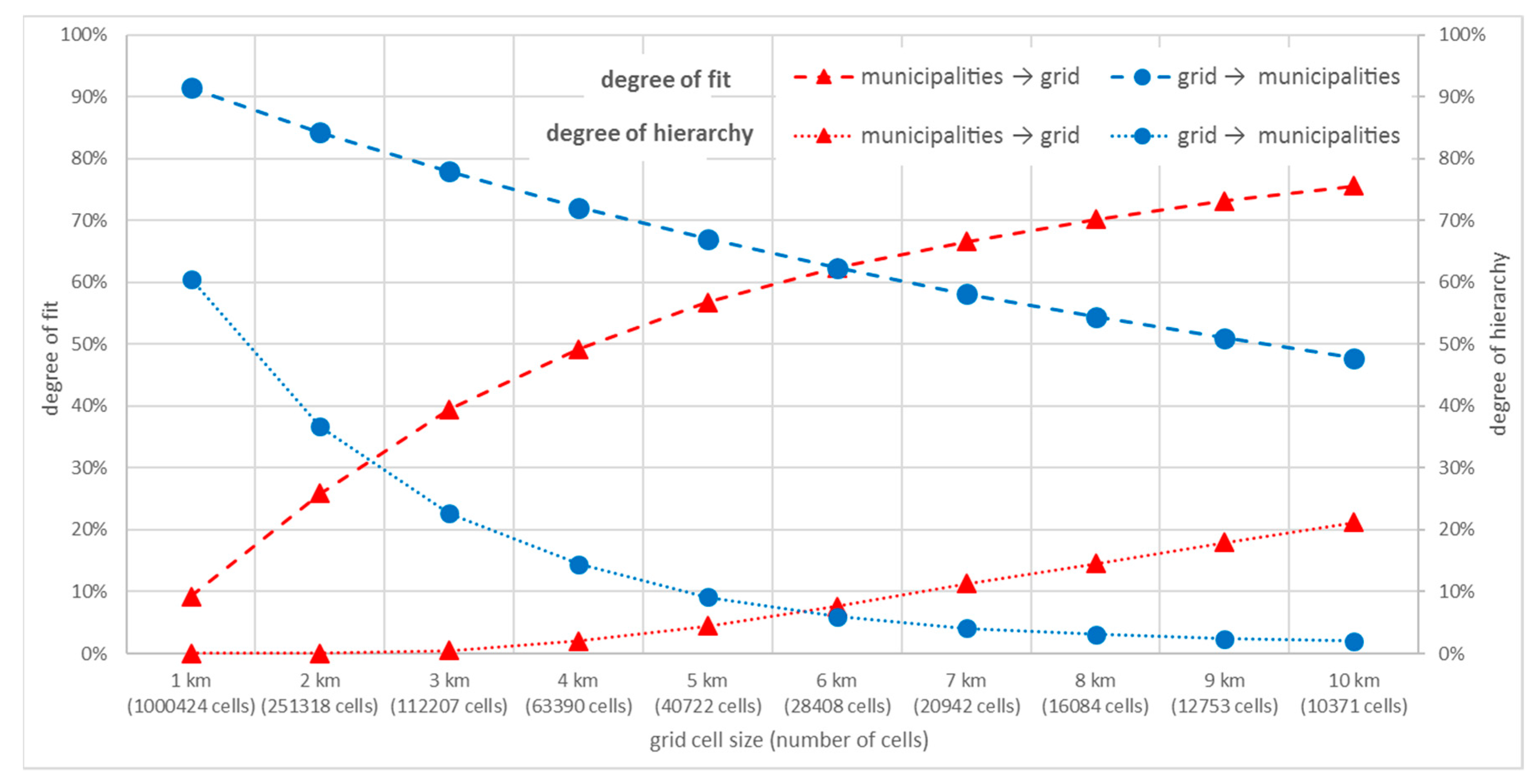
We use the two Simpson’s measures to estimate the ‘goodness of fit’ between the real regional structure of municipalities and regular structures with different grid sizes changing from 1 to 10 km with a lag of 1 km. The resulting values of the degree of hierarchy and the degree of fit for 10 different grid structures are depicted in Figure 3. Based on the number of cells (close to the number of municipalities, 28,937) and the highest balance between the degree of fit for grid-to-municipalities and municipalities-to-grid directions, we recommend using the grid with cells of 6 × 6 km for this particular region. The choice of the 6 km grid is visible by the intersection of the municipalities-to-grid and grid-to-municipalities graphs of both the degree of fit and the degree of hierarchy. When increasing or decreasing the size of the cells, the degree increases in one direction but significantly decreases in the other; the goal is to maximize both directions of the degree.
In Table 3, the goodness of fit statistics for municipal structure and the 6 km grid in all studied countries can be seen. From these figures, the differences in regional structure are clear, Poland and Czechia being the biggest outliers. In Czechia, the very fragmented regional structure is documented by a relatively low degree of fit in the grid-to-municipalities direction (municipalities are smaller than the grid). In Poland, the least fragmented structure from the studied countries is documented by a relatively low degree of fit in the municipalities-to-grid direction (municipalities are bigger than the grid). However, the chosen grid size of 6 km has the best average degree of fit for both directions and all studied countries.
Still, there might be a problem with the exact placement of the regular grid. Thus, we have tested different placements of the grid according to the degree of fit. We shifted the 6 km grid by 1 km each direction (both x and y axes) and tested 36 possible grid placements. For each 6 km grid placement, we measured the degree of fit for both directions (municipalities-to-grid and grid-to-municipalities). The resulting values of the degree of fit measured are not significantly different (with the maximum degree of fit being 62.44, minimum 62.18, and mean 62.31). Thus, we may conclude that the grid placement is not important for our results.
When data are in a regular grid, we can analyse the data using standard spatial methods such as local spatial autocorrelation. Spatial autocorrelation helps to identify the spatial pattern of unemployment, possible spatial clusters or development axes. In this paper, we use hot spot analysis, specifically the Getis–Ord (Gi*) spatial statistic [23,24]. It visualizes high-high and low-low types of clusters (on different significance levels) and identifies statistically significant hot spots and cold spots. To constitute a statistically significant hot spot, a phenomenon with a high value should also be surrounded by other phenomena with high values. When using hot spot analysis, the concept of proximity is important. The proximity is decided upon using spatial weights. The spatial weighting scheme defines which units (municipalities, in our case) are considered close for the calculation of the hot spot analysis. The choice of a different spatial weight may influence the final results. For a discussion about the importance of spatial weights, see [25]. Although the selection of a particular spatial weighting scheme is arbitrary and influences the final results, based on the evidence from the literature [25], we do not consider this issue to be important. The importance of spatial weight is also diminished by the areal interpolation that adjusted the data before we performed the hot spot analysis. In this paper, we use queen contiguity (1st order) in the hot spot analysis.
4. Empirical Results
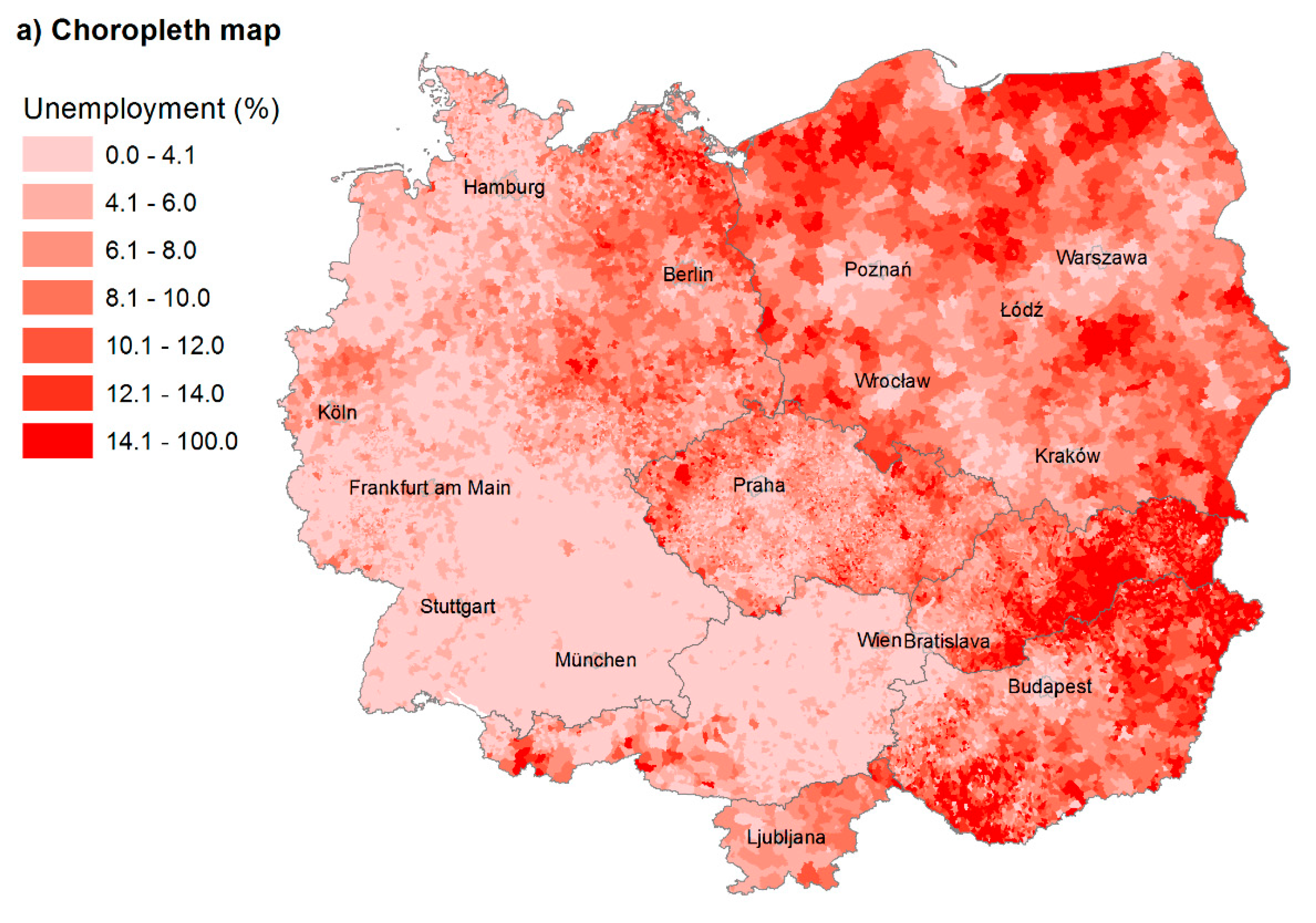
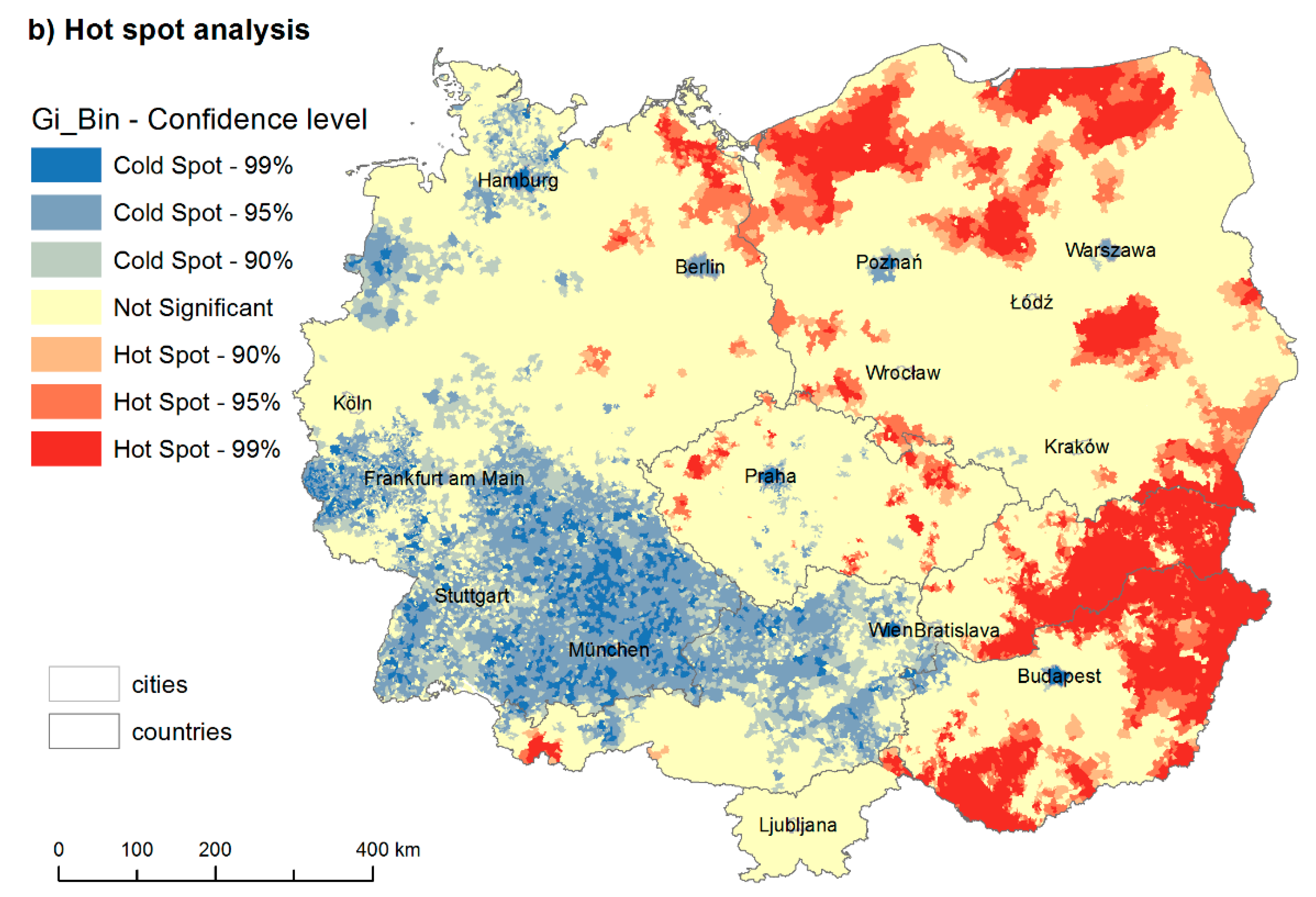
First, the spatial patterns of unemployment in the CER region are visualised by a choropleth map (see Figure 4a). There are 28,937 municipalities. Even from this simple visualization, a sharp difference between unemployment in the west and east is visible, as well as more favourable unemployment levels in bigger agglomerations. However, the map is rather fragmented and, apart from the mentioned results, difficult to interpret. The bigger units dominate and attract our attention (such as Polish municipalities or bigger cities). Moreover, different sizes of municipalities in studied countries do not allow the interpretation of cross-border clusters.
After having the unemployment surface, we can proceed with hot spot analysis, namely the Getis–Ord (Gi*) spatial statistic [23,24]. The hot spot analysis is presented in the form of a cluster map (Figure 4b). For example, if we have the unemployment data, we can study whether unemployment values are more similar in close municipalities. If they are, the positive spatial autocorrelation is present and a cluster (high-high or low-low types) forms. If the values are randomly distributed in space, there is no spatial autocorrelation. We treat the whole CER as one system, thus with one mean.
The cold spots (blue) depict the low level of unemployment, while the hot spots (red) depict high levels of unemployment. The west-east divide is still visible. However, while the border between former Western Germany and Eastern Germany is fuzzy, the German-Czech border from the Bavarian side and the Austria-Czech border are very sharp, one exception being the low-low axis stretching from Prague. This historical border seems to have high inertia. Moreover, since unemployment is connected with the labour market, the border is significantly sharper in the case of national borders with a language barrier (Germany-Czechia and Austria-Czechia).
The western bloc forms a huge low-low cluster with one exception- the Ruhr region, which has a high-high cluster with a higher unemployment rate. In the rest of the region, there are large high-high clusters with low-low pockets around population centres. There are cold spots of low unemployment in bigger agglomerations in all countries east of this divide (Berlin, Prague, Poznan, Warsaw, Wroclaw, Krakow, Bratislava, Budapest, Ljubljana) and hot spots of high unemployment in problematic areas such as eastern Slovakia, eastern and south-western Hungary, or north-western and north-eastern Poland. There might even be development axes forming between the biggest agglomerations. One axis stretches from Prague to Germany and Austria in the south and Wroclaw and Poznan in the north. Within Poland, there are proto-axes between Warsaw, Krakow, Wroclaw and Poznan. From Poznan, it can then stretch further towards Berlin and link Poland to the Blue Banana [26]. However, the results would need to be studied over a longer interval to examine these effects.
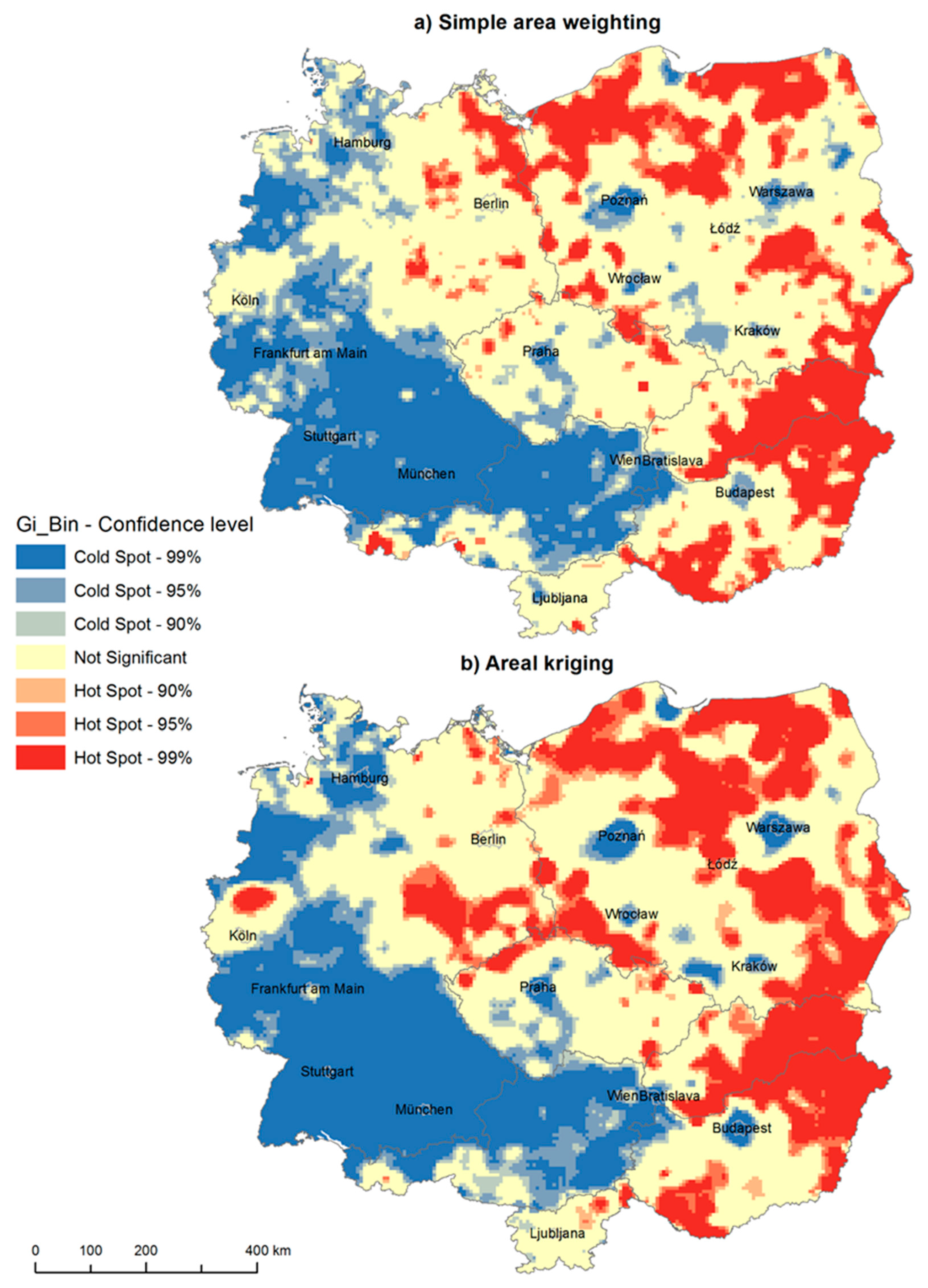
Figure 5 shows the results of hot spot analysis of the unemployment computed in the 6 km regular grid with 28.395 squares using areal interpolation. When using areal interpolation, the resulting surface is smoother; it dissolves the small municipalities with extreme values, such as a municipality with a 100% unemployment rate while having one unemployed inhabitant. Thus, the overall picture is clearer. The comparison between cluster maps based on simple area weighting and areal kriging demonstrates the difference between the computation of these two methods. In simple area weighting, people (population 15–64 and unemployed) were simply being redistributed. In areal kriging the method is searching for a model which smooths out the results; it does not show extremes as significantly as the simple weighting method. Thus, the resulting map obtained by the areal kriging method is more compact (with fewer isolated clusters) and easier to interpret. The west-east divide and cold spots in bigger agglomerations are even more visible when compared to the results obtained by the simple weighting method.
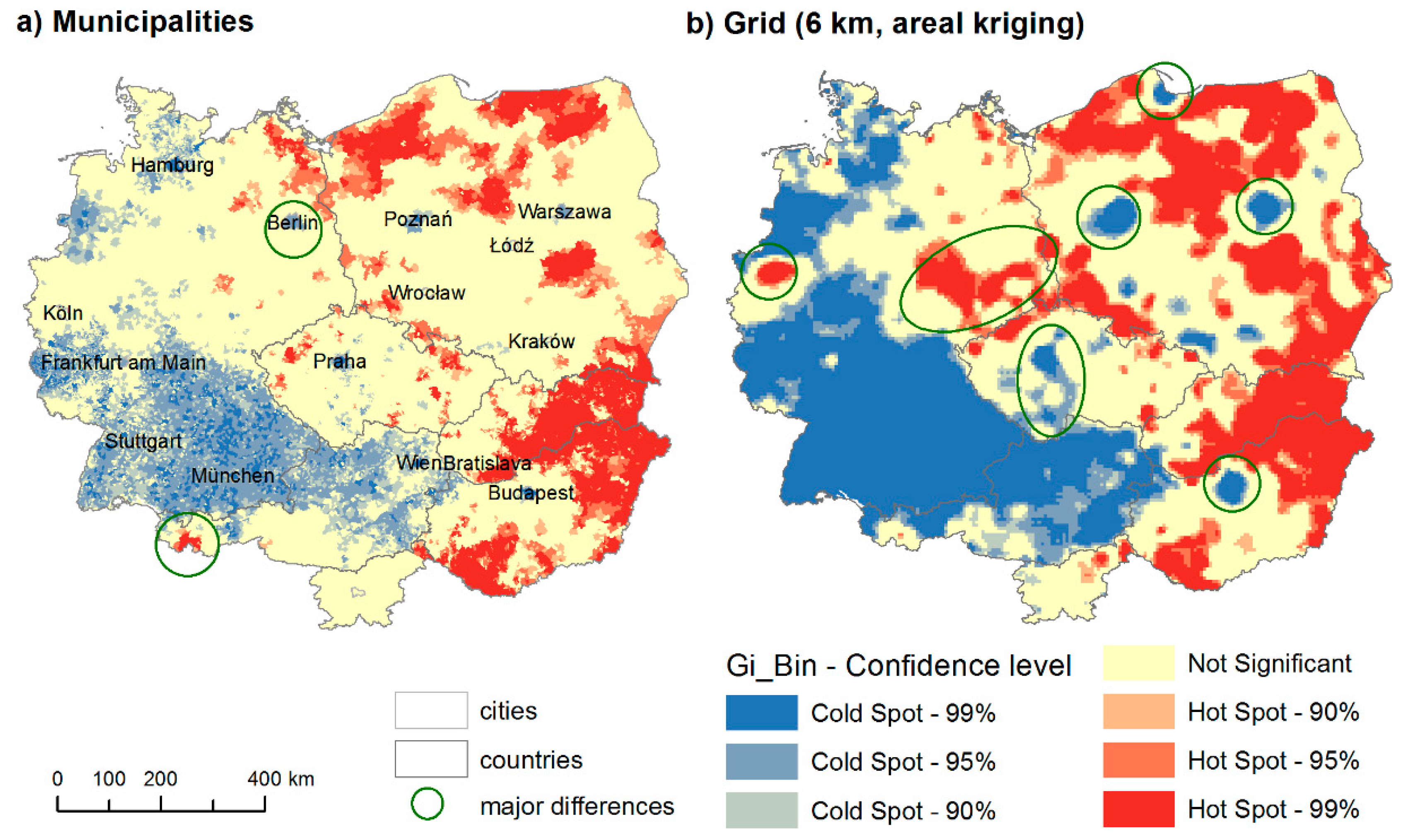
The difference between the hot spot analysis of unemployment in municipalities and grid (6 km, areal kriging) nicely captures where this methodology does not add much value and where it significantly improves the final interpretation (see Figure 6). When the differences are rather big (such as in case of West-East difference in unemployment), the hot-spot analysis or even a simple choropleth map is usually sufficient. However, if the differences are not that big (such as in unemployment in Czechia, Slovakia, and Poland), the areal interpolation (areal kriging in this case) provides us with a more accurate description of the reality. The results are not that affected by the outliers, be it extreme values in some municipalities, or extremely small or large municipalities. The main differences are highlighted in Figure 6. The analyses demonstrate the huge empirical potential of the areal interpolation method in international research. In particular, the method seems to be suitable to study potential development axes.
From an empirical point of view, the performed analyses shed new light on empirical international research concerning border issues. As Petrakos and Topaloglou [27] put it, it is unclear whether border regions inherently benefit from cross-border cooperation, or whether they remain peripheral regions that are not profoundly affected by economic and political integration despite their close geographic location. When using unemployment rate as a proxy for economic development [28], national borders still seem to be more of a barrier than a bridge. This is probably connected with the dependency of unemployment on the labour market, which is difficult to form across national borders, especially when there is a language barrier [29]. It may be hypothesized that different economic characteristics (such as GDP) could be less affected by the national border. On the other hand, income levels would probably be connected to labour markets, much like unemployment. Thus, national borders could have a strong effect.
5. Conclusions
The main goal of the paper was to introduce a strategy on how to deal with the regional comparability issue, which is one of many general issues connected with comparability [3]. Addressing this issue is especially important in international research. It is connected with two situations: (i) differing regional structures of two or more different systems (such as countries), and (ii) changing regional structures in time (changes in regional delimitations). We have introduced a strategy utilizing areal interpolation to better homogenize differing regional structures to a grid structure. This approach enables us to make spatial data analyses effective.
Every data transformation generates error influenced by differences between source units and target units. First, it is important to choose the most suitable target structure (such as a regular grid), the size of the units, and its position. To do so, we propose using two measures; the degree of hierarchy (nesting) and the degree of fit (overlap) [16]. These two measures express the error involved in the transformation from source to target units. Usually, these measures are used to quantify the goodness of fit between the given source and target structure. However, if you need to select the most suitable target structure, we propose using a two-way fit (source-to-target and target-to-source) and selecting the target structure with the maximum average fit. In the example of the Central European region and municipalities as a source structure, we chose a 6 km grid in a specific position based on this approach. For a different region or different source units, one can find its best grid size and position using the same approach.
Second, we applied two methods of areal interpolation most suitable for our research, (i) simple area weighting and (ii) areal kriging. We have shown how to correctly implement these methods and discussed the most important issues connected to them. The standard spatial analyses methods, such as hot spot analysis, proved to be more suitable for analysing spatial phenomena than non-spatial methods (see the choropleth map difference). The areal interpolation methods are even more suitable in international regional research. Compared to other methods (such as a choropleth map and hot spot analysis based on municipal data), several important advantages were identified. First of all, areal interpolation does not bring many new insights in cases where the differences of two or more systems (countries) are big, such as in case of the overall difference between West and East. However, in cases where the differences are not that visible, areal interpolation can significantly change the final interpretation. This is visible when the maps created by municipality hot spot analysis and areal kriging are compared. It is specifically important in regions with major regional centres (such as big cities in Poland), which have significantly different sizes. In general, areal interpolation methods are not that affected by outliers (both in terms of extreme values and in terms of extremely different spatial sizes). For our purposes and goals, areal kriging was the best option. However, this does not have to be the same if the research goals are different.
Moreover, there are many potential cases for this methodology to be used in empirically oriented research. It’s important to remember that the analysis, as presented in this paper, should be performed in a time series to assess the evolution of spatial patterns. The harmonisation of geographical zones is essential to a time-series of estimates because boundaries change over time. The temporal inconsistencies in regional boundaries is a big practical issue in geographical evolutionary analyses. Specifically, in Europe, the numbers and boundaries of municipalities continue to change over time. Areal interpolation enables conversion of regional structure backwards and forwards in time and thus constitute a consistent regional system [17]. The suggested methodology can be effectively used for the interpretation of evolutionary dynamics.
From an empirical point of view, the Central European region is very interesting because of the changing role of the borders studied. Special attention may be given to the emergence of development axes throughout the Central European region. Moreover, different characteristics should be used, especially those less affected by institutions with higher inertia, such as labour markets. The challenge is to find sufficiently spatially detailed data for this kind of analysis. Some more detailed focus can be given to national borders within the Eastern Bloc or elsewhere where the historical heritage is not as strong as in the case of the Iron Curtain. In addition to national borders, other types of borders could be studied. For example, there are many historical borders within the studied region. On top of that, after performing quantitative analyses, further explanatory research is necessary to uncover the causal relations behind the identified patterns.
Author Contributions
Pavlína Netrdová and Vojtěch Nosek conceived and designed the study, analysed the data and wrote the paper; Pavol Hurbánek provided help in data collection and analysis. All authors read and approved the final manuscript.
Funding
This research was funded by the Czech Science Foundation (GACR), grant number 18-20904S, and by the Charles University Research Centre program UNCE/HUM/018.
Conflicts of Interest
The authors declare no conflict of interest.
References
- Burkhauser, R.V.; Lillard, D.R. The contribution and potential of data harmonization for cross-national comparative research. J. Comp. Policy Anal. Res. Pract. 2005, 7, 313–330. [Google Scholar] [CrossRef] [Green Version]
- Idrizi, B. General Conditions of Spatial Data Infrastructure. Int. J. Nat. Eng. Sci. 2018, 12, 57–62. [Google Scholar]
- Bonaccorsi, A.; Daraio, C.; Lepori, B.; Slipersaeter, S. Indicators on individual higher education institutions: Addressing data problems and comparability issues. Res. Eval 2007, 16, 66–78. [Google Scholar] [CrossRef]
- Arbia, G. Statistical Effect of Data Transformations: A Proposed General Framework. In The Accuracy of Spatial Data Bases; Goodchild, M.F., Gopal, S., Eds.; Taylor and Francis: London, UK, 1989; pp. 249–259. ISBN 978-0850668476. [Google Scholar]
- Arntz, M.; Wilke, R. An application of cartographic area interpolation to German administrative data. Asta-Adv. Stat. Anal. 2007, 91, 159–180. [Google Scholar] [CrossRef]
- Lu, S.; Guan, X.; Yu, D.; Deng, Y.; Zhou, L. Multi-scale analysis of regional inequality based on spatial field model: A case study of China from 2000 to 2012. Isprs Int. J. Geo-Inf. 2015, 4, 1982–2003. [Google Scholar] [CrossRef] [Green Version]
- Gotway, C.A.; Young, L.J. Combining incompatible spatial data. J. Am. Stat. Assoc 2002, 97, 632–648. [Google Scholar] [CrossRef] [Green Version]
- Hallisey, E.; Tai, E.; Berens, A.; Wilt, G.; Peipins, L.; Lewis, B.; Graham, S.; Flanagan, B.; Buchanan Lunsford, N. Transforming geographic scale: A comparison of combined population and areal weighting to other interpolation methods. Int J. Health Geogr. 2017, 16, 29. [Google Scholar] [CrossRef] [Green Version]
- Qiu, F.; Zhang, C.; Zhou, Y. The development of an areal interpolation ArcGIS extension and a comparative study. Gisci. Remote Sens. 2012, 49, 644–663. [Google Scholar] [CrossRef]
- Jega, I.M.; Comber, A.J.; Tate, N.J. A Comparison of Methods for Spatial Interpolation across Different Spatial Scales. Ssrg Int. J. Geoinf. Geol. Sci. 2017, 4, 12–22. [Google Scholar]
- Goodchild, M.F.; Lam, N.S.-N. Areal interpolation: A variant of the traditional spatial problem. Geo-Process. 1980, 1, 297–312. [Google Scholar]
- Li, T.; Pullar, D.; Corcoran, J.; Stimson, R. A comparison of spatial disaggregation techniques as applied to population estimation for South East Queensland (SEQ), Australia. Appl. Gis 2007, 3, 1–16. [Google Scholar]
- Krivoruchko, K.; Gribov, A.; Krause, E. Multivariate Areal Interpolation for Continuous and Count Data. Procedia Environ. Sci. 2011, 3, 14–19. [Google Scholar] [CrossRef] [Green Version]
- Deichmann, U.; Balk, D.; Yetman, G. Transforming Population Data for Interdisciplinary Usages: From Census to Grid; Socioeconomic Data and Applications Center (CIESIN, Columbia): New York, NY, USA, 2001; Available online: https://sedac.ciesin.columbia.edu/gpw-v2/GPWdocumentation.pdf (accessed on 3 March 2019).
- Dawson, T.; Sandoval, J.S.O.; Sagan, V.; Crawford, T. A Spatial Analysis of the Relationship between Vegetation and Poverty. Isprs Int. J. Geo-Inf. 2018, 7, 83. [Google Scholar] [CrossRef] [Green Version]
- Simpson, L. Geography conversion tables: A framework for conversion of data between geographical units. Int J. Popul Geogr. 2002, 8, 69–82. [Google Scholar] [CrossRef]
- Norman, P.; Rees, P.; Boyle, P. Achieving Data Compatibility over Space and Time: Creating Consistent Geographical Zones. Int. J. Popul. Geogr. 2003, 9, 365–386. [Google Scholar] [CrossRef] [Green Version]
- Bláha, J.D.; Nováček, A. How Central Europe is Perceived and Delimited. Mitt. Osterr. Geogr. Ges. 2016, 158, 193–214. [Google Scholar] [CrossRef]
- Openshaw, S. The Modifiable Areal Unit Problem (CATMOG 37); Geo Books: Norwich, UK, 1984; p. 41. [Google Scholar]
- Wong, D.W.S. The Modifiable Areal Unit Problem (MAUP). In The SAGE Handbook of Spatial Analysis; Fotheringham, A.S., Rogerson, P.A., Eds.; SAGE: London, UK, 2009; pp. 105–123. [Google Scholar]
- Nelson, J.K.; Brewer, C.A. Evaluating data stability in aggregation structures across spatial scales: Revisiting the modifiable areal unit problem. Cartogr. Geogr. Inf. Sci. 2017, 44, 35–50. [Google Scholar] [CrossRef]
- Netrdová, P.; Nosek, V. Exploring the variability and geographical patterns of population characteristics: Regional and spatial perspectives. Morav. Geogr. Rep. 2017, 25, 85–94. [Google Scholar] [CrossRef] [Green Version]
- Getis, A.; Ord, J.K. The Analysis of Spatial Association by Use of Distance Statistics. Geogr. Anal. 1992, 24, 189–206. [Google Scholar] [CrossRef]
- Ord, J.K.; Getis, A. Local Spatial Autocorrelation Statistics: Distributional Issues and an Application. Geogr. Anal. 1995, 27, 286–306. [Google Scholar] [CrossRef]
- Nosek, V.; Netrdová, P. Measuring Spatial Aspects of Variability. Comparing Spatial Autocorrelation with Regional Decomposition in International Unemployment Research. Hist. Soc. Res. 2014, 39, 292–314. [Google Scholar] [CrossRef]
- Netrdová, P.; Nosek, V. Spatial patterns of unemployment in Central Europe: Emerging development axes beyond the Blue Banana. J. Maps 2016, 12, 701–706. [Google Scholar] [CrossRef]
- Petrakos, G.; Topaloglou, L. Economic geography and European integration: The effects on the EU’s external border regions. Int J. Public Pol. 2008, 3, 146–162. [Google Scholar] [CrossRef]
- Lewandowska-Gwarda, K. Geographically Weighted Regression in the Analysis of Unemployment in Poland. Isprs Int. J. Geo-Inf. 2018, 7, 17. [Google Scholar] [CrossRef] [Green Version]
- Boussauw, K.; Van Meeteren, M.; Sansen, J.; Meijers, E.; Storme, T.; Louw, E.; Derudder, B.; Witlox, F. Planning for agglomeration economies in a polycentric region: Envisioning an efficient metropolitan core area in Flanders. Eur. J. Spat. Dev. 2018, 69, 1–26. [Google Scholar] [CrossRef]
Figure 1.
Calculations of the percentage of overlay the degree of fit, municipalities-to-grid and grid-to-municipalities directions. Source: © EuroGeographics for the administrative boundaries, European Commission, Eurostat/GISCO.
Figure 1.
Calculations of the percentage of overlay the degree of fit, municipalities-to-grid and grid-to-municipalities directions. Source: © EuroGeographics for the administrative boundaries, European Commission, Eurostat/GISCO.

Figure 2.
The Central European region under study. Source: © EuroGeographics for the administrative boundaries, European Commission, Eurostat/GISCO.
Figure 2.
The Central European region under study. Source: © EuroGeographics for the administrative boundaries, European Commission, Eurostat/GISCO.

Figure 3.
Degree of fit and degree of hierarchy between the regional structure of municipalities and the grid structures with different grid cell sizes.
Figure 3.
Degree of fit and degree of hierarchy between the regional structure of municipalities and the grid structures with different grid cell sizes.

Figure 4.
Choropleth map (a) and hot spot analysis (b) of unemployment in 2010 in municipalities in CER. Source: © EuroGeographics for the administrative boundaries, European Commission, Eurostat/GISCO.
Figure 4.
Choropleth map (a) and hot spot analysis (b) of unemployment in 2010 in municipalities in CER. Source: © EuroGeographics for the administrative boundaries, European Commission, Eurostat/GISCO.


Figure 5.
Hot spot analysis of unemployment in a 6 km grid, simple area weighting (a) and areal kriging (b). Source: © EuroGeographics for the administrative boundaries, European Commission, Eurostat/GISCO.
Figure 5.
Hot spot analysis of unemployment in a 6 km grid, simple area weighting (a) and areal kriging (b). Source: © EuroGeographics for the administrative boundaries, European Commission, Eurostat/GISCO.

Figure 6.
Comparison of hot spot analysis of unemployment in municipalities (a) and grid (b—6 km, areal kriging). Source: © EuroGeographics for the administrative boundaries, European Commission, Eurostat/GISCO.
Figure 6.
Comparison of hot spot analysis of unemployment in municipalities (a) and grid (b—6 km, areal kriging). Source: © EuroGeographics for the administrative boundaries, European Commission, Eurostat/GISCO.


Table 1.
Municipalities (LAU2 units) in studied countries.
| Country | Number | Original Name | Average Area (km2) | Population 15–64 Years | |
|---|---|---|---|---|---|
| Mean | Median | ||||
| Austria | 2357 | Gemeinde | 35.6 | 2373.1 | 1045.5 |
| Czechia | 6250 | Obce | 12.6 | 1189.8 | 292.5 |
| Germany | 11,563 | Gemeinde | 30.9 | 4661.3 | 1075.0 |
| Hungary | 3152 | Települések | 29.5 | 2245.0 | 587.0 |
| Poland | 2478 | Gminy | 126.2 | 11,036.4 | 5223.0 |
| Slovakia | 2927 | Obce | 16.8 | 6763.8 | 448.0 |
| Slovenia | 210 | Občine | 96.5 | 1307.0 | 3335.0 |
| Total | 28,937 | - | 34.4 | 3684.2 | 771.0 |
Source: own calculation based on data from official statistical sources in studied countries—Statistik Austria (http://www.statistik.at/), Czech Statistical Office (http://www.czso.cz/), Statistische Ämter des Bundes und der Länder (https://www.regionalstatistik.de/genesis/online/data), Hungarian Central Statistical Office (https://www.teir.hu/), Central Statistical Office of Poland (http://www.stat.gov.pl), Statistical Office of the Slovak Republic (http://www.statistics.sk), Statistical Office of the Republic of Slovenia (http://www.stat.si/).
Table 2.
Unemployment in studied countries.
| Country | Number of Registered Unemployed People | Unemployment 1 | Unemployment 1 in Municipalities | ||
|---|---|---|---|---|---|
| Mean | Median | Range | |||
| Austria | 244,923 | 4.32 | 3.7 | 3.0 | 37.5 |
| Czechia | 482,719 | 6.54 | 6.6 | 6.1 | 100.0 |
| Germany | 2,938,392 | 5.45 | 4.0 | 3.3 | 23.9 |
| Hungary | 545,411 | 7.78 | 11.2 | 9.8 | 44.3 |
| Poland | 1,942,756 | 7.10 | 8.3 | 7.9 | 22.8 |
| Slovakia | 382,314 | 9.85 | 13.8 | 11.2 | 72.2 |
| Slovenia | 102,026 | 7.18 | 7.3 | 7.0 | 12.3 |
| Total | 6,638,541 | 6.23 | 6.7 | 5.2 | 100.0 |
1 Unemployment = number of registered unemployed people in October 2010 (from official statistical sources in studied countries) normalized by the working-age population (15–64) on 31 December 2010. Due to data availability, the number of registered unemployed people in Poland and Slovakia is for December 2010 instead of October 2010. Source: own calculation based on data from official statistical sources in studied countries—Statistik Austria (http://www.statistik.at/), Czech Ministry of Labour and Social Affairs (http://www.mpsv.cz/), Czech Statistical Office (http://www.czso.cz/), Statistik der Bundesagentur für Arbeit (http://statistik.arbeitsagentur.de), Statistische Ämter des Bundes und der Länder (https://www.regionalstatistik.de/genesis/online/data), National Employment Service (http://en.munka.hu/), Hungarian Central Statistical Office (https://www.teir.hu/), Central Statistical Office of Poland (http://www.stat.gov.pl), Central Office of Labour, Social Affairs and Family (http://www.upsvr.gov.sk/), Statistical Office of the Slovak Republic (http://www.statistics.sk), Statistical Office of the Republic of Slovenia (http://www.stat.si/).
Table 3.
Goodness of fit statistics for municipal structure and 6 km regular grid in respective countries.
Table 3.
Goodness of fit statistics for municipal structure and 6 km regular grid in respective countries.
| Country | Number of Municipalities | Number of Cells | Degree of Fit | Degree of Hierarchy | ||
|---|---|---|---|---|---|---|
| M 1 → G 1 | G → M | M → G | G → M | |||
| Austria | 2357 | 2544 | 58.5% | 61.8% | 3.7% | 6.7% |
| Czechia | 6250 | 2369 | 73.5% | 46.4% | 15.2% | 4.5% |
| Germany | 11,563 | 10,457 | 62.3% | 60.2% | 7.3% | 5.2% |
| Hungary | 3152 | 2751 | 62.6% | 58.8% | 4.6% | 5.3% |
| Poland | 2478 | 8983 | 31.3% | 75.0% | 0.3% | 11.7% |
| Slovakia | 2927 | 1498 | 68.6% | 48.6% | 8.3% | 3.3% |
| Slovenia | 210 | 660 | 39.5% | 78.1% | 0.0% | 21.8% |
1 M = municipalities, G = 6 km grid.
© 2020 by the authors. Licensee MDPI, Basel, Switzerland. This article is an open access article distributed under the terms and conditions of the Creative Commons Attribution (CC BY) license (http://creativecommons.org/licenses/by/4.0/).
Share and Cite
MDPI and ACS Style
Netrdová, P.; Nosek, V.; Hurbánek, P. Using Areal Interpolation to Deal with Differing Regional Structures in International Research. ISPRS Int. J. Geo-Inf. 2020, 9, 126. https://0-doi-org.brum.beds.ac.uk/10.3390/ijgi9020126
AMA Style
Netrdová P, Nosek V, Hurbánek P. Using Areal Interpolation to Deal with Differing Regional Structures in International Research. ISPRS International Journal of Geo-Information. 2020; 9(2):126. https://0-doi-org.brum.beds.ac.uk/10.3390/ijgi9020126
Chicago/Turabian StyleNetrdová, Pavlína, Vojtěch Nosek, and Pavol Hurbánek. 2020. "Using Areal Interpolation to Deal with Differing Regional Structures in International Research" ISPRS International Journal of Geo-Information 9, no. 2: 126. https://0-doi-org.brum.beds.ac.uk/10.3390/ijgi9020126
Note that from the first issue of 2016, this journal uses article numbers instead of page numbers. See further details here.