Lattice Quad-Tree Indexing Algorithm for a Hexagonal Discrete Global Grid System


1
PLA Strategic Support Force Information Engineering University, Zhengzhou 450001, China
2
The Army of 31617, Fuzhou 350201, China
*
Author to whom correspondence should be addressed.
ISPRS Int. J. Geo-Inf. 2020, 9(2), 83; https://0-doi-org.brum.beds.ac.uk/10.3390/ijgi9020083
Submission received: 7 November 2019
/
Revised: 22 January 2020
/
Accepted: 27 January 2020
/
Published: 31 January 2020
(This article belongs to the Special Issue Global Grid Systems)
Abstract
:Hexagonal discrete global grid systems are the preferred data models supporting multisource geospatial information fusion. Related research has aroused widespread concern in the academic community, and hierarchical indexing algorithms are one of the main research focuses. In this paper, we propose an algorithm for indexing the cell of a ringed spatial area based on a hexagonal lattice quad-tree (HLQT) structure and the indexing characteristics. First, we design a single-resolution indexing algorithm in which indexing starts from the initial quad tree and expands ring by ring using coding operations, and a quad-tree structure is applied to accelerate this process. Second, the hierarchical indexing algorithm is implemented based on single-resolution indexing, and a pyramid hierarchical model is established. Finally, we perform comparison experiments with existing algorithms. The results of the experiments indicate that the single-level indexing efficiency of the proposed algorithm is approximately twice that of the traditional method and that the hierarchical indexing efficiency is approximately 67 times that of the traditional method. These findings verify the feasibility and superiority of the algorithm proposed in this paper.
1. Introduction
In recent years, the application of geospatial data has become increasingly extensive. The scale, shape, projection and reference datum of these data are extremely varied, which makes the aggregation, processing and mining of datasets extremely difficult [1]. A demand has been identified for establishing a new data association model that uses spatial locations as the primary key by which to encode and integrate/fuse multisource location-based information [2]. The traditional model of geographic information system (GIS), in which GIS experts process and integrate data, is unsustainable in the face of the ever-increasing flow of data [1].
A discrete global grid system (DGGS) uses a specific method to discretize the Earth uniformly to form a seamless and multiresolution grid hierarchy structure using cell codes instead of traditional geographic coordinates to perform data operations [1,2,3,4]. A DGGS resembles a spreadsheet of cells over the surface of the Earth [2]. This approach promotes timely data analysis, processing, and reuse, and it preserves the appropriate information for multisource geodata mining. Additionally, this method can quickly and seamlessly assimilate new high-volume or disparate geodata sources and sensor networks regardless of scale, origin, resolution, legacy format, datum, or projection [1,2].
The planar quadrilateral grid system has a direct connection with the quad-tree data structure, and the quadrature-based indexing algorithm is directly applicable [5]. However, on a spherical surface, a quadrilateral DGGS is severely deformed at high latitudes, and the grid cells at the north and south poles are degenerated into triangles that must be treated differently from other cells. Moreover, quadrilaterals do not exhibit uniform adjacency, which increases the complexity of spatial analysis [6]. Gorski et al. established a quadrilateral discrete global grid framework called HEALPix (Hierarchical Equal Area isoLatitude Pixelation of a Sphere) for the efficient discretization and fast analysis/synthesis of functions defined on a sphere [6,7]. GeoFusion divides the globe into six regions, of which four are covered by rectangular grids between 45 degrees north and south and two are covered by triangular grids at high latitudes [8]. Australia’s SEE-Grid (Solid Earth and Environment Grid) system is built based on cubes using quadrilateral grids and is mainly used for environmental monitoring [9]. Bernardin et al. built a quadrilateral grid system called Crusta that started from a 30-sided rhombic triacon-tahedron to support high-resolution topography data and imagery [10]. Lambers et al. established the quadrilateral grid system ellipsoidal cube map (ECM), which uses one-to-four refinement on the faces of a cube that circumscribes an ellipsoidal Earth [11]. Cheng et al. proposed the geographical coordinate subdividing grid with one-dimension integer coding on a tree (GeoSOT) grid coding scheme, which is mainly used for the organization and management of remote-sensing data [12].
Triangular grids can establish connections with the quad-tree model and have high rendering efficiency for visualization. However, the unit adjacency relationship changes considerably at different positions, which requires complex neighboring search and spatial analysis algorithms. Dutton proposed the quaternary triangular mesh (QTM) model based on a regular octahedron structure and designed a hierarchical indexing method [13]. Goodchild’s hierarchical spatial data structure (HSDS) system also provides global estimates using an octahedron structure with one-to-four triangular refinement [14]. Bartholdi and Goldsman established a successive global indexing mechanism based on the spherical triangle hierarchy [15]. Zhao proposed the degenerate quad-tree grid (DQG) and designed the corresponding coding scheme and neighboring search algorithm [16].
Hexagon structures have received a great deal of interest because of their advantages. Among the three types of regular polygons that tile the plane (triangles, quads, and hexagons), hexagons are the most compact [3], and they provide the greatest angular resolution [17]. Unlike square and triangle grids, hexagonal grids have uniform adjacency, which means that each hexagonal cell has six neighbors, and all the neighbors share an edge with the hexagon and have centers exactly the same distance away from its center [3]. Vince established the octahedral aperture 3 hexagonal discrete global grid system, for which coordinate-based indexing based on barycentric coordinates is used to index the cells [18]. Ben et al. improved the model to develop the indexing system of the octahedral aperture 4 hexagonal discrete global grid system [19]. Peterson, Vince et al. designed the hierarchical indexing scheme PYXIS for the icosahedral Snyder equal area aperture 3 hexagon (ISEA3H), implemented a Fourier transform algorithm and developed spatial data integration software for the real-time processing and analysis of multisource datasets [20,21,22]. Sahr proposed a similar hierarchy-based approach using coordinate-based pyramid indexing based on hexagonal coordinate systems [23]. The pyramidal scheme, however, was only developed for a single resolution [1]. Sahr proposed the concept of a mixed-aperture hexagonal grid system combining multiple apertures. He designed the central place indexing (CPI) scheme [24] and implemented the basic algorithm in DGGRID [25,26]. Tong et al. proposed the hexagonal quaternary balanced structure (HQBS) [27] and established the hierarchical relationships among different levels of hexagonal grids on the icosahedral triangle. However, operations frequently roll back when code normalization fails, resulting in low efficiency [28]. Mahdavi-Amiri et al. designed a hierarchical indexing and visualization scheme for a variety of hexagonal grids based on a special coordinate system on a diamond surface [29]. To take advantage of the advantages of different types of grids, Mahdavi-Amiri [30] proposed a conversion method among hexagonal, quadrilateral and triangular grids for better storing and rendering. Hexagons do not exhibit congruency, and it is thus impossible to exactly decompose a hexagon into smaller hexagons [3]. Therefore, it is difficult to apply efficient multiresolution hierarchical indexing algorithms and quad-tree data structures on a hexagonal DGGS directly. To address this issue, Wang et al. established a hexagonal lattice quad-tree structure (HLQT) encoding scheme based on the theory of complex radix numbers [31]. A quad-tree data structure was applied for hierarchical representation and basic operations with hexagonal grids, but research on hierarchical indexing has not yet been performed.
In summary, recent studies on grid modeling and code indexing for DGGSs have made great progress. Quadrilateral and triangular DGGSs have direct correlations with the quad-tree data structure. The existing efficient indexing algorithms can be directly transformed, but these types of DGGSs do not have uniform adjacency characteristics, and the cell deformation is severe at high latitudes; thus, such methods are not suitable for the organization and processing of global spatial data. Hexagonal grids have ideal uniform adjacency properties and the advantage of evenly covering the entire world; however, they do not have self-similarity properties. Therefore, most results cannot be generalized to the quad-tree data structure. Aiming to address the current research gaps, this paper designs an indexing algorithm based on HLQT that accelerates indexing using code operations and the structural characteristics of the quad tree. The efficiency and reliability of the scheme are validated by comparison experiments.
2. Encoding Scheme of HLQT
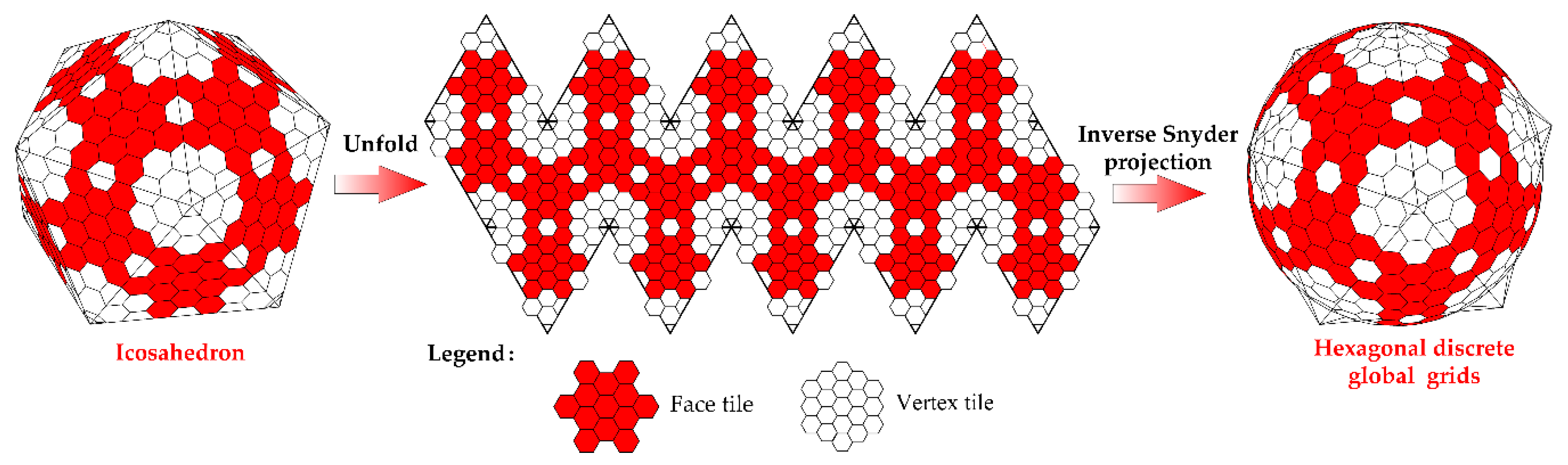
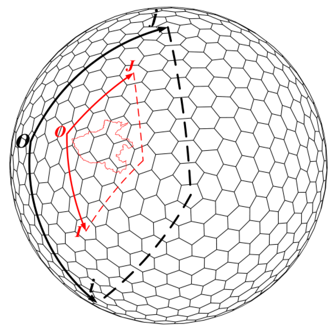
Wang et al. established a planar HLQT encoding scheme [31]. Vince et al. [32] and Ben et al. [28] divided the aperture 3 DGGS into two segments (vertex tile and face tile) according to the boundary of the icosahedron and achieved uniform, global aperture 3 hexagonal grid encoding. According to this concept, an icosahedral HLQT encoding scheme can also be established [33], and a Snyder polyhedral projection is used to map the surface of the icosahedron to the sphere [34]. The tile structure is shown in Figure 1.
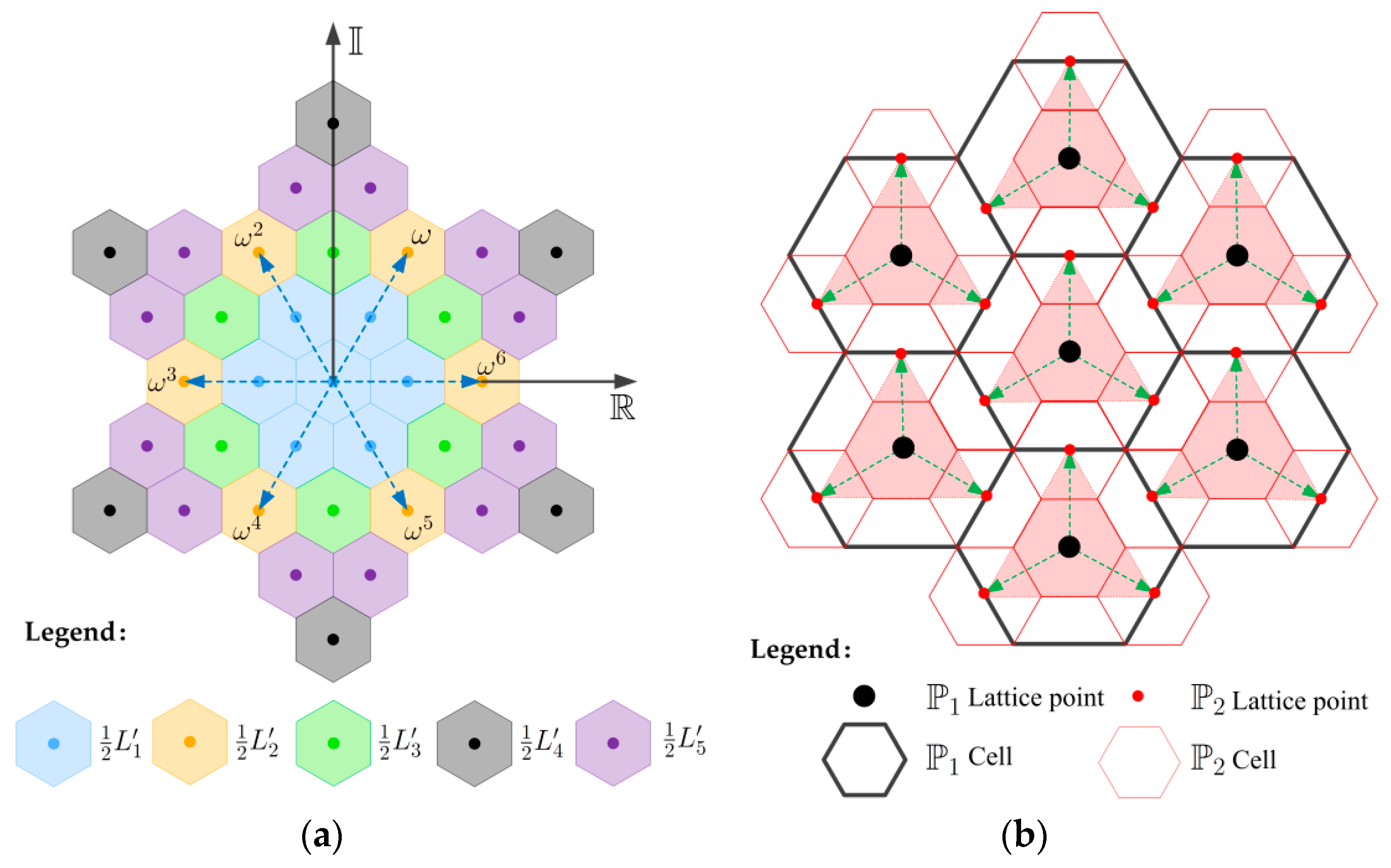
In Figure 1, the face tile structure on the icosahedral triangle face is identical, and the vertex tile is a partial expurgation and expansion based on the face tile. We define the center of the cell as the lattice point to replace the cell equivalently and let denote the lattice points of level . We define the first-level lattice points as shown in Figure 2a. Each lattice point generates four child lattice points, and are generated in turn. As shown in Figure 2b, is obtained by generating four child lattice points from independently, and thus the hierarchy structure constitutes a quad tree.
As shown in Figure 2a, on the complex plane, we let (where is an imaginary unit), and is represented by the following five sets ():
- ;
- ;
- ;
- ; and
- or or .
Additionally, we let , . After a rigorous proof, the set of lattice points of the 4-aperture hexagonal grid system can be uniquely represented as follows:
In Formula (1), . Formula (1) shows that the aperture 4 hexagonal lattice system is essentially a counting system in which lattices are numbers with a specific form in the complex field and are exactly the same as the binary and decimal numbers in the real number field. The counting system has a binary value of two, and the sets of digits are and . For , the specific form is shown in Formula (2).
Similar to a decimal number, by omitting the power exponent, Formula (2) can be expressed as shown in Formula (3).
We replace in Formula (3) according to the following rules:
- (1)
- For , let ;
- (2)
- for , let ;
- (3)
- for , ;
- (4)
- for , are the code digits after the replacement of ); and
- (5)
- for , .
- (6)
- Similarly, we replace with .
- (7)
- Digital set is replaced with the coded digit set , and digital set is replaced with the coded digit set . The unique identifier for is shown in Formula (4).
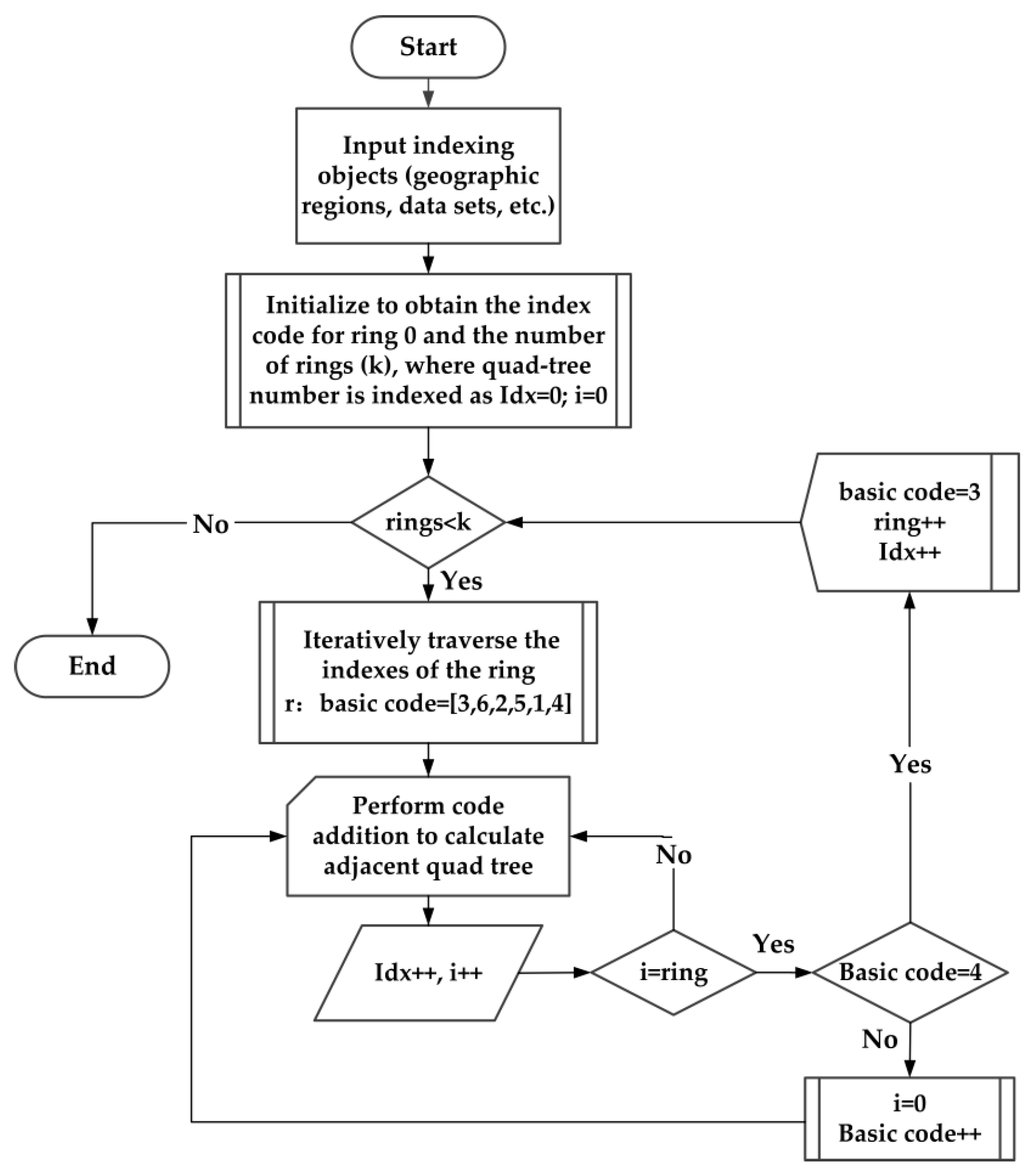
According to the complex radix vector addition principle, the code addition table is defined. An example of a coding addition operator is shown in Figure 3.
3. Indexing Algorithm
The basic method of spatial indexing is to divide the whole space into different search areas and find spatial entities in these areas in a certain order. The face tiles and vertex tiles in HLQT divide the globe into different search areas, and the separate processing approach is used for indexing. The focus of this paper is a proposed single-level and hierarchical indexing algorithm based on tiles. Due to the equivalence of coding schemes between tiles, such an indexing algorithm is applicable to a wide range of regions, including the entire globe [28].
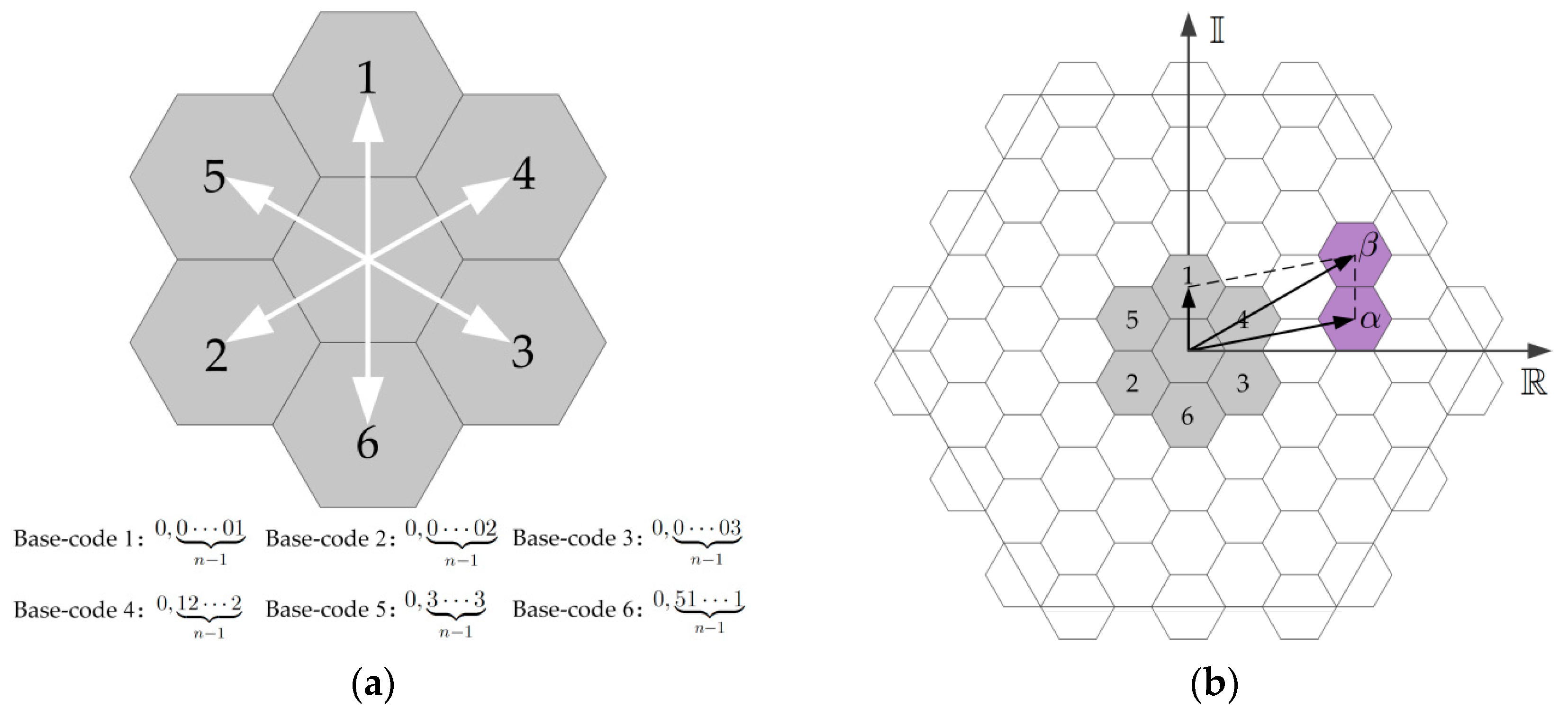
Indexing addition operations avoid floating-point operations and improve the efficiency of searching cells. Based on this method, this paper designs a code addition structure consisting of the central cell code of a tile and the surrounding six cell codes (hereinafter referred to as the base codes, numbered 1–6); these codes are related to the hierarchical structure. The code addition structure of level n is shown in Figure 4a. According to the HLQT coding operation scheme, the neighboring cells of any cell in a tile can be calculated by addition. As shown in Figure 4b, the adjacent cell of in a tile can be obtained by adding the base code 1 to , and the surrounding cell codes can similarly be calculated by addition.
3.1. Single-Resolution Indexing Algorithm
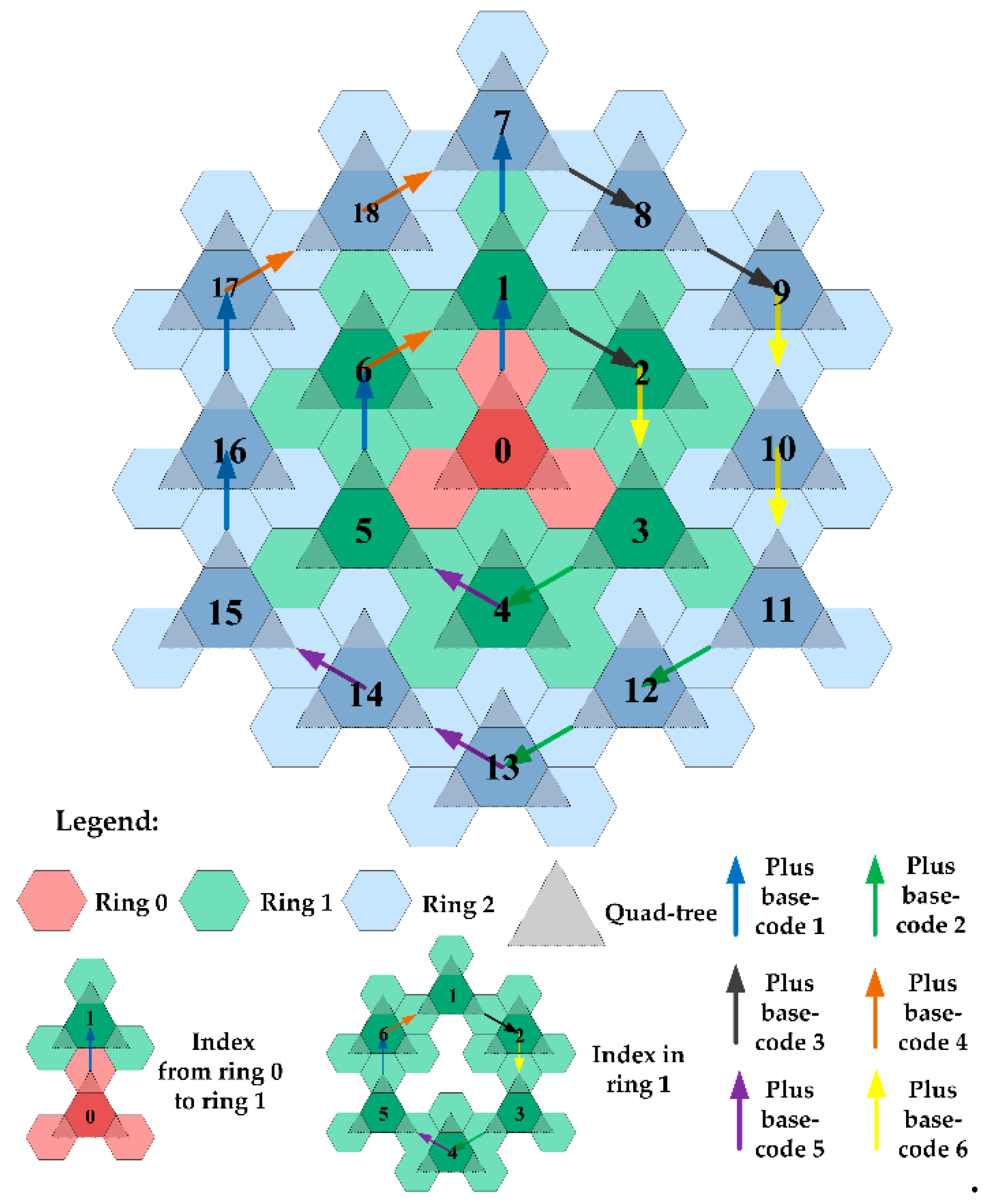
We design an indexing algorithm that starts from an initial quad tree and grows outward ring by ring. The code addition operation is used between adjacent quad trees, and only the last digit of the cells on the tree must be changed, which considerably improves the indexing efficiency. The index structure is shown in Figure 5.
As shown in Figure 5, the indexing algorithm makes full use of the HLQT quad-tree structure. Ring 0 is the initial indexing quad-tree, and cells are searched ring by ring according to a specific algorithm. Except for ring 0, ring is composed of (6 ✕ ) quad trees. The indexing process is divided into two parts: indexing between rings and indexing within a ring. The specific indexing algorithm performs four steps as follows:
- (1)
- Input the objects (geographic regions, data sets, etc.) to be indexed; then, initialize the data to obtain the ring 0 indexes and the number of rings, denoted as .
- (2)
- Index the next ring. The first quad tree of the next ring is obtained by adding the base code 1 to the quad tree of the previous ring. In Figure 5, the indexing of the initial quad tree to that of the first and the indexing of first quad tree to that of the seventh are examples of indexing between rings.
- (3)
- Traverse the indexes of ring . Each ring needs to complete quad-tree transitions in six different directions corresponding to the six basic codes of the code addition structure; for example, for the first ring, the transitions are . Note that for ring , the addition operation is performed in each direction times. As shown in Figure 4, in Ring 1, indexing the first quad tree to that of the second requires one addition, and for Ring 2, indexing the seventh quad tree to that of the ninth requires two additions.
- (4)
- Repeat Step (3) while the number of rings < .
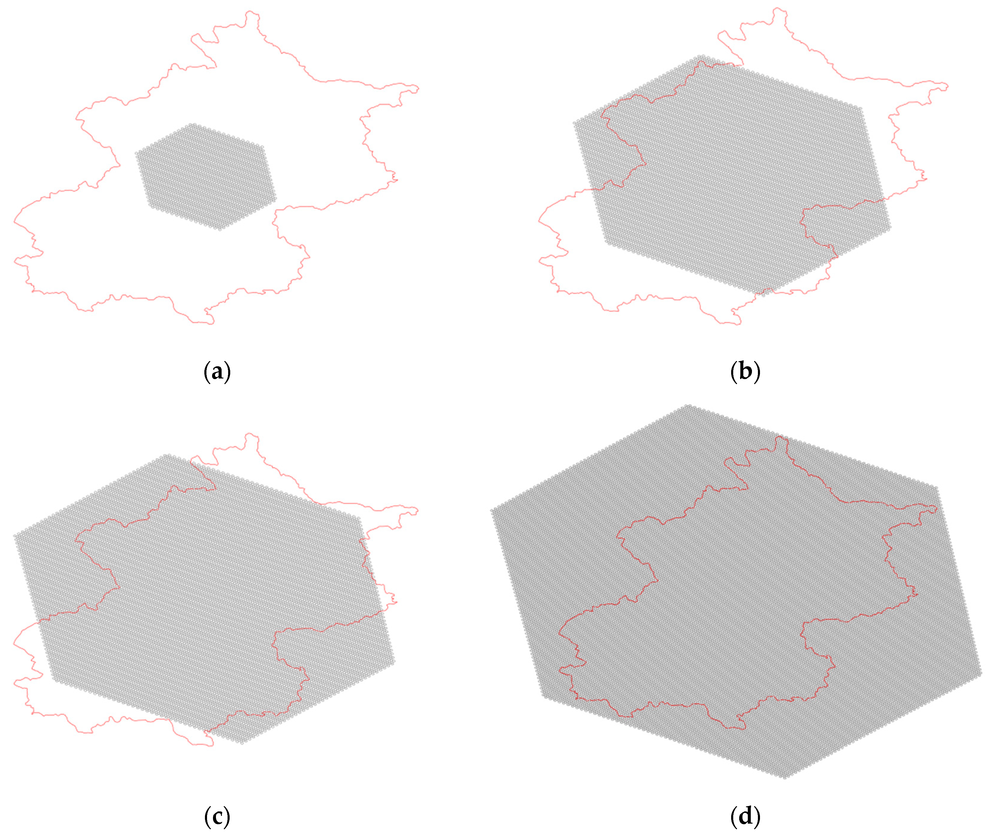
Taking Beijing, China, as an example, the level of the grid system is 13. The cell codes are obtained according to the above indexing algorithm. We record the indexing results at four different moments and convert them into grids, which are displayed in Figure 6. The entire algorithm process is shown in Figure 7.
3.2. Hierarchical Indexing Algorithm
The indexing algorithm of the ringed space region is implemented above, but this approach is only for a single resolution, and there is no connection between grid levels. In multiresolution operations, such as data zooming, it is necessary to convert between coarse and fine grids in real time, and an efficient hierarchical indexing algorithm plays an important role in this process. This paper implements different levels of indexing based on single-level ringed-region indexing. The specific algorithm employs the following steps:
- (1)
- Enter an object (data set or administrative division) and index it according to the single-level indexing algorithm (Figure 7) at the initial grid resolution.
- (2)
- When performing a zoom-in operation for the object, each cell at the initial resolution generates a quad-tree that includes four children cells. Then, the cell is indexed to a higher level, as shown in Figure 8b.
- (3)
- Continue with Step (2) until the grids of the highest level are all indexed.
- (4)
- When a zoom-out operation is performed for an object, each quad tree of the high-resolution grid degenerates to the parent cell of the previous level, and this iterative process continues until the coarsest grids are all indexed.
The hierarchical indexing algorithm is essentially a quad-tree algorithm that only involves the addition and culling of the last coded digit, and no full code addition operation is required. Only when the index is being determined at the initial resolution is a single-level indexing algorithm needed.
4. Experiments and Analysis
4.1. Data Indexing with a Large Scope
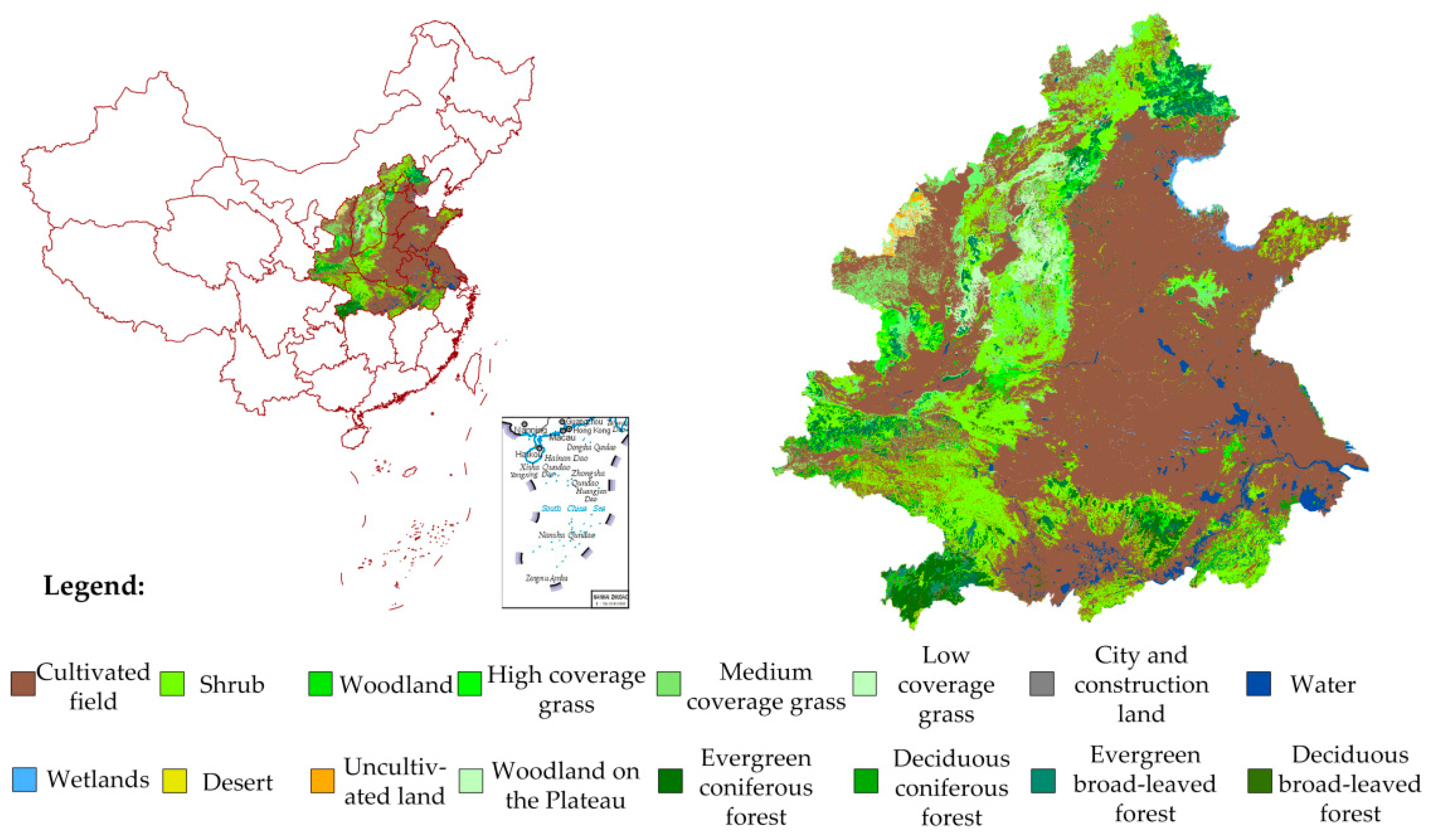
The experimental data used in this paper includes Chinese vegetation coverage grid data obtained from the Resource and Environmental Science Data Center of the Chinese Academy of Sciences in 2000. The data are in the Albers equal area conic projection, and the size of each grid is 1 x 1 km. We selected ten provinces and cities in China (Hebei, Beijing, Tianjin, Shandong, Jiangsu, Anhui, Hubei, Shanxi, Shanxi, and Henan Provinces) for testing; there were 1,204,186 sampling points, as shown in Figure 9.
We design a comparative experiment to verify the efficiency of the proposed indexing algorithm. It has been demonstrated [31] that the efficiency of the code addition operations of HLQT is higher than those of HQBS and PYXIS. Therefore, the indexing algorithm proposed in this paper is more efficient than HQBS and PYXIS because we use the coding structure of the quad tree to accelerate the index operations; thus, we do not make an efficiency comparison here.
Mahdavi-Amiri et al. [29] designed a hierarchical indexing scheme named “connectivity maps” for hexagonal grids; this scheme combined the two triangular faces of icosahedrons as diamonds and used the diamonds as the basic object for 3, 4 or 7-aperture refinement. The work in this paper uses the tile structure on the icosahedron as the basic refinement object (Figure 1); the refinement scheme of each tile is the same, and the refinement aperture is 4. The connectivity maps yielded considerable improvements in indexing neighborhood and hierarchical cells, and the diamond structure facilitated visualization. Neighborhood search operations were simply performed by adding neighborhood vectors to the index of a hexagon, and hierarchical cell searching was performed by multiplying R or R (scalar) by the index of a given cell (where R represents a rotation, scaling or translation matrix). In the proposed indexing scheme, adjacent cells can be quickly obtained by code addition, as shown in Figure 4. Hierarchical cell searching only needs to increase or decrease one digit at the end of the code.
Sahr used an scheme for the indexes of the hexagonal grid cells in the open source project DGGRID [25,26]. Adjacent searching is the advantage based on row and column codes, and this comparison can reflect the effectiveness of the proposed indexing scheme. Sahr combined icosahedral triangles into 10 quads to process each quad separately. The indexing scheme constructs a minimum outsourced quadrilateral geographic area in each quadrilateral (the example in Figure 10 is Henan Province, China), as shown in Figure 10.
The basic steps in the DGGRID indexing algorithm can be summarized as follows.
(1) Convert the data from latitude and longitude to codes (where is the quadrilateral number), and calculate the extremums of and to obtain and The lower left coordinate of the minimum outsourced quadrilateral is denoted as , and the upper right coordinate is denoted as for the given data range.
(2) Convert the data from latitude and longitude to again, and translate the coordinate axis to narrow the index range and obtain the minimum outsourced quadrilateral, as shown in Figure 10. The Formula (5) is for obtaining the new code:
(3) Index the smallest outsourced quad and convert it to the actual codes in the original coordinate system.
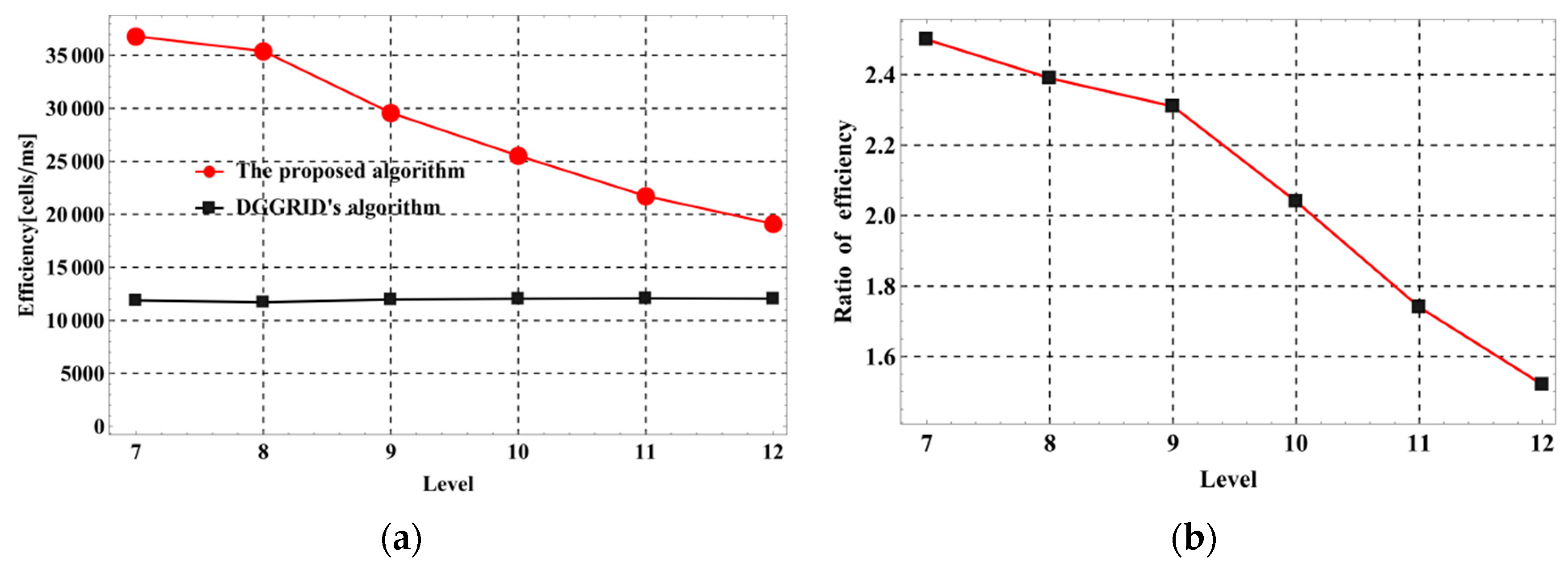
To ensure fair and objective comparisons, the icosahedral positioning parameters [3] are selected to ensure that the grids do not cross the surface. The indexing time is recorded at the respective resolutions. Calculations are repeated ten times and then averaged, and the number of indexing cells in each level is calculated. Finally, the efficiency is determined as the number of cells indexed per millisecond. The results are shown in Table 1 and Table 2, and the efficiency comparison curves are shown in Figure 11 and Figure 12. Each program was compiled for the release version and operated on the same desktop (Core [email protected] GHz six-core CPU, 8G RAM WDC WDS480G2G0A-00JH30 480G SSD; Windows 7 X64 Ultimate SP1; development software: Microsoft Visual C++ 2012 Update 5).
The results of the comparison experiment indicate that the efficiency of the proposed algorithm is higher than that of the DGGRID algorithm. The average efficiency of single-level indexing is approximately two times that of the DGGRID algorithm, and the average efficiency of hierarchical indexing is approximately 67 times higher. The reasons for these results are as follows:
- (1)
- The DGGRID encoding method uses numbers, and its major advantage is proximity searching [4]. However, in the case of cell indexing for regions, because codes must be indexed in sequence, a small outsourced quadrilateral, as shown in Figure 10, must be determined to narrow the indexing range to reduce memory consumption, which requires multiple conversion calculations, resulting in decreased efficiency.
- (2)
- The proposed algorithm does not need to perform sequential indexing and only needs to “know” the center coordinates and index range of the object. Thus, the code operations and coding structure of the quad tree accelerate the indexing process. As the level increases, the frequency of code addition increases, and the length of the code digit becomes longer, resulting in a decrease in efficiency, as shown in Figure 11.
- (3)
- A main feature of the hierarchical indexing algorithm in this paper is the establishment of quad-tree relationships between levels. When indexing via the proposed approach, we only need to add or subtract a digit at the end of the code, whereas the DGGRID method does not use hierarchical information [25], and the minimum quadrilateral range of the next level must be calculated. Moreover, the number of indexing cells is large, as shown in Table 2. Therefore, the proposed algorithm is superior, as shown in Figure 12a, but as the level increases, the HLQT code length increases, resulting in a higher cost of code digit processing. As a result, the efficiency ratio decreases, as shown in Figure 12b.
- (4)
- For large-scale, including global, data processing in practical applications, level-of-detail (LOD) processing is often adopted [35]. The range of high-resolution regions close to the viewpoint is small, resulting in a small number of cells. The resolution far from the viewpoint is low, and the proposed algorithm has a higher indexing efficiency when the grid resolution is low; therefore, the algorithm in this paper is advantageous in practical applications.
4.2. Data Indexing with a Small Scope
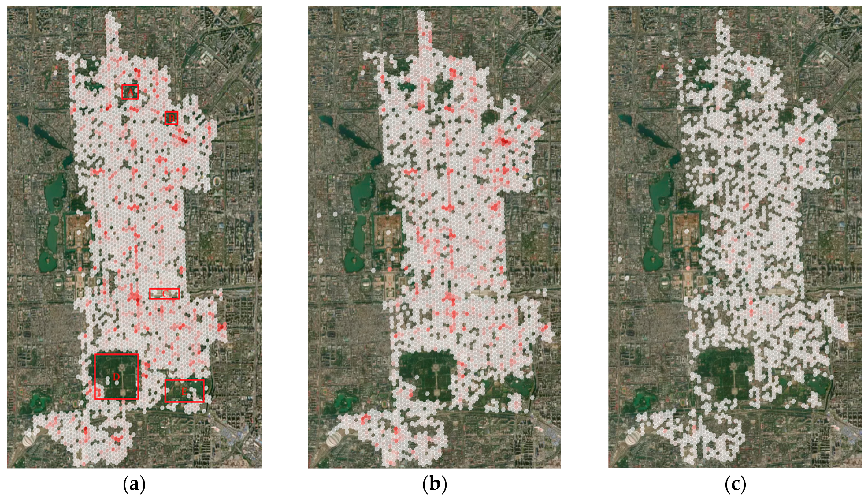
Similarly, our indexing algorithm can be applied for indexing small-scope data, such as bike-sharing data in cities. Although the scope of bike-sharing data is small, the data are constantly updated, resulting in a large amount of data. Therefore, the timely and effective analysis of the data is particularly important. In this experiment, the bike-sharing data from Dongcheng district in Beijing were provided by Beijing Engineering Laboratory of Beidou Navigation and LBS Technology [36]. We select different periods of a working day for experiments, and the grid level is set to 17. We then convert the latitude and longitude coordinates of the data into codes, and the number of bikes in each cell is counted. Finally, different depths of color are assigned to the cells according to the number of bikes present (the more bikes there are, the darker the color is). We index the codes using our single-resolution indexing algorithm (Figure 5) and render hexagon data on a web map. The results of the experiments are shown in Figure 14.
The following analysis can be obtained from the above experiments:
- (1)
- (2)
- The distribution of bikes in different time periods is basically the same. Therefore, companies should add bikes in areas with dark colors, as shown in Figure 14.
- (3)
- Parking in areas A to E (Figure 14a) is prohibited; as a result, there are few bikes in these areas. If there are bikes in these areas, the company should promptly find and remove them.
While used in indexing and analyzing such dynamic, changing data, hexagons are a desirable choice. Hexagons can minimize the quantization error introduced when bikes move through a city; since the edge or length of contact is the same on each side, the centroid of each neighbor is equidistant; finding neighbors is more straightforward using a hexagon grid. Our hexagonal indexing algorithm accelerates the neighborhood searching by code addition operation and quad-tree gird structure, which is conducive to dynamic data indexing and visual analysis. Moreover, our algorithm index a ringed region that is similar to a circle, which allows us to approximate radiuses easily and is beneficial for searching the surrounding bikes.
5. Conclusions and Future Research Directions
In this paper, we design a ringed-region indexing algorithm based on HLQT using code addition operations and a quad-tree structure to accelerate hierarchical indexing. The comparison experiments verify the feasibility and efficiency of the proposed algorithm, with the proposed algorithm not only improving the efficiency of the single-resolution indexing method but also significantly improving the indexing efficiency among multiresolution levels.
By using hexagonal grids to organize and manage multiple spatial data, the indexing algorithm proposed in this paper can quickly and accurately index multi-resolution data with a specified ring region. We give two potential application scenarios: (a) In a GIS spatial analysis, we may search for data located n kilometers around a certain position, such as in the case of clients looking for hotels within three kilometers or taxi users querying taxis within five kilometers. Because the main advantage of the algorithm provided in this paper is hierarchical indexing, we can first index the ringed area at a lower resolution, and then we can perform hierarchical indexing from coarse to fine to determine the target position. (b) In the visual analysis of multi-resolution spatial data, the algorithm presented in this paper can display data at multiple levels via its efficient hierarchical indexing.
However, the proposed algorithm only considers the situation for a single tile. When the object range is large, the trans-surface cells must be processed separately. This topic will be a focus of our future research.
Author Contributions
Conceptualization, Jianbin Zhou, Jin Ben and Rui Wang; Methodology, Jianbin Zhou; Software, Jianbin Zhou and Jin Ben; Validation, Jianbin Zhou, Rui Wang and Mingyang Zheng; Formal Analysis, Jianbin Zhou and Lingyu Du; Investigation, Lingyu Du, Rui Wang; Resources, Mingyang Zheng; Data Curation, Jin Ben; Writing—Original Draft Preparation, Jianbin Zhou and Jin Ben; Writing—Review & Editing, Jianbin Zhou and Jin Ben; Visualization, Jianbin Zhou and Jin Ben; Supervision, Jin Ben. All authors have read and agreed to the published version of the manuscript.
Funding
This research was funded by the Natural Science Foundation of China, grant number [41671410].
Conflicts of Interest
The authors declare no conflict of interest.
References
- Mahdavi-Amiri, A.; Alderson, T.; Samavati, F. A survey of digital earth. Comput. Graph. 2015, 53, 95–117. [Google Scholar] [CrossRef]
- Peterson, P.R. Discrete Global grid systems. Int. Encycl. Geogr. People Earth Environ. Technol. 2016, 1–10. [Google Scholar] [CrossRef]
- Sahr, K.; White, D.; Kimerling, A.J. Geodesic discrete global grid systems. Cartogr. Geogr. Inf. Sci. 2003, 30, 121–134. [Google Scholar] [CrossRef] [Green Version]
- Mahdavi-Amiri, A.; Samavati, F.; Peterson, P. Categorization and Conversions for Indexing Methods of Discrete Global Grid Systems. ISPRS Int. J. Geo-Inf 2015, 4, 320–336. [Google Scholar] [CrossRef]
- Samet, H. Foundations of Multidimensional and Metric Data Structures; Morgan Kaufmann Publishers Inc.: San Francisco, CA, USA, 2005. [Google Scholar]
- Gorski, K.M.; Hivon, E.; Banday, A.J.; Wandelt, B.D.; Hansen, F.K.; Reinecke, M.; Bartelmann, M. HEALPix: A framework for high-resolution discretization and fast analysis of data distributed on the sphere. Astrophys. J. 2005, 622, 759. [Google Scholar] [CrossRef]
- Hivon, E.; Gorski, K.M.; Reinecke, M. HEALPix-Data Analysis, Simulations and Visualization on the Sphere. Available online: https://sourceforge.net/projects/healpix/ (accessed on 10 October 2019).
- GeoFusion. GeoMatrix Toolkit Programmer’s Manual. Available online: http://www.geofusion.com/ (accessed on 12 October 2019).
- SEEGrid. WebHome SCENZGrid SEEGrid. Available online: https://www.seegrid.csiro.au/wiki/SCENZGrid/WebHome (accessed on 12 October 2019).
- Bernardin, T.; Cowgill, E.; Kreylos, O.; Bowles, C.; Gold, P.; Hamann, B.; Kellogg, L. Crusta: A new virtual globe for real-time visualization of sub-meter digital topography at planetary scales. Comput. Geosci. 2011, 37, 75–85. [Google Scholar] [CrossRef]
- Lambers, M.; Kolb, A. Ellipsoidal Cube Maps for Accurate Rendering of Planetary-Scale Terrain Data. Cg.informatik.uni 2012. [Google Scholar] [CrossRef]
- Cheng, C. The global subdivision grid based on extended mapping division and its address coding. Acta Geod. Cartogr. Sin. 2010, 39, 295–302. [Google Scholar] [CrossRef] [Green Version]
- Dutton, G. A Hierarchical Coordinate System for Geoprocessing and Cartography; Springer: Berlin, Germany, 1999. [Google Scholar]
- Goodchild, M.F.; Shiren, Y. A Hierarchical Spatial Data Structure for Global Geographic Information Systems (89-5). Ncgia Nat. Center Geogr. Inf. Anal. 1989, 54, 31–44. [Google Scholar] [CrossRef] [Green Version]
- Bartholdi, J.J.; Goldsman, P. Continuous indexing of hierarchical subdivisions of the globe. Int. J. Geogr. Inf. Sci. 2001, 15, 489–522. [Google Scholar] [CrossRef] [Green Version]
- Zhao, X.; Cui, M.; LI, A.; Zhang, M. An Adjacent Searching Algorithm of Degenerate Quadtree Grid on Spherical Facet. Geomat. Inf. Sci. Wuhan Univ. 2009, 34, 479–482. [Google Scholar] [CrossRef]
- Golay, M.J.E. Hexagonal parallel pattern transformations. IEEE Trans. Comput. 1969, 100, 733–740. [Google Scholar] [CrossRef]
- Vince, A. Indexing the aperture 3 hexagonal discrete global grid. J. Vis. Commun. Image Represent. 2006, 17, 1227–1237. [Google Scholar] [CrossRef]
- Ben, J.; Tong, X.C.; Zhou, C.H.; Zhang, K.X. Construction algorithm of octahedron based hexagon grid systems. J. Geo-Inf. Sci. 2015, 6, 54–61. [Google Scholar] [CrossRef]
- PYXIS Innovation Inc. How PYXIS Works. Available online: http://www.pyxisinnovation.com/pyxwiki/index.php?title (accessed on 12 October 2019).
- Peterson, P. Closed-Packed Uniformly Adjacent, Multi-Resolutional Overlapping Spatial Data Ordering. U.S. Patent #0,8018,458, 13 September 2011. [Google Scholar]
- Vince, A.; Zheng, X.X. Arithmetic and fourier transform for the PYXIS multi-resolution digital earth model. Int. J. Digit. Earth 2009, 2, 59–79. [Google Scholar] [CrossRef]
- Sahr, K. Location coding on icosahedral aperture 3 hexagon discrete global grids. Comput. Environ. Urban Syst. 2008, 32, 174–187. [Google Scholar] [CrossRef]
- Sahr, K. Central place indexing: Hierarchical linear indexing systems for mixed-aperture hexagonal discrete global grid systems. Cartographica 2019, 54, 16–29. [Google Scholar] [CrossRef]
- Sahr, K. DGGRID Version 6.4: User Documentation for Discrete Global Grid Generation Software. Available online: http://webpages.sou.edu/~sahrk/docs/dggridManualV64.pdf (accessed on 12 October 2019).
- Sahr, K. DGGRID Users. Available online: https://www.discreteglobalgrids.org/dggrid-users/ (accessed on 12 October 2019).
- Tong, X.C.; Ben, J.; Wang, Y.; Zhang, Y.S.; Pei, T. Efficient encoding and spatial operation scheme for aperture 4 hexagonal discrete global grid system. Int. J. Geogr. Inf. Sci. 2013, 27, 898–921. [Google Scholar] [CrossRef]
- Ben, J.; Li, Y.L.; Zhou, C.H.; Wang, R.; Du, L.Y. Algebraic encoding scheme for aperture 3 hexagonal discrete global grid system. Sci. China Earth Sci. 2018, 61, 215–227. [Google Scholar] [CrossRef]
- Mahdavi-Amiri, A.; Harrison, E.; Samavati, F. Hexagonal connectivity maps for Digital Earth. Int. J. Digit. Earth 2014, 8, 750–769. [Google Scholar] [CrossRef]
- Mahdavi-Amiri, A.; Harrison, E.; Samavati, F. Hierarchical grid conversion. Comput. Aided Des. 2016, 79, 12–26. [Google Scholar] [CrossRef]
- Wang, R.; Ben, J.; Du, L.Y.; Zhou, J.B.; Li, Z.X. Encoding and operation for the planar aperture 4 hexagon grid system. Acta Geotech. Cartogr. Sin. 2018, 47, 1018–1025. [Google Scholar] [CrossRef]
- Vince, A. Indexing a discrete global grid. In Special Topics in Computing and ICT Research, Advances in Systems Modelling and ICT Applications; Fountain Publishers: Kampala, Uganda, 2006; Volume 2, pp. 3–17. [Google Scholar]
- Wang, R.; Ben, J.; Du, L.Y.; Zhou, J.B.; Li, Z.X. The code operation scheme for the icosahedral aperture 4 hexagon grid system. Geomat. Inf. Sci. Wuhan Univ. 2019. [Google Scholar] [CrossRef]
- Snyder, J.P. An Equal-Area Map Projection For Polyhedral Globes. Cartographica 1992, 29, 10–21. [Google Scholar] [CrossRef]
- Sußner, G.; Dachsbacher, C.; Greiner, G. Hexagonal LOD for Interactive Terrain Rendering. In Proceedings of the Vision Modeling and Visualization, Erlangen, Germany, 16–18 November 2005; pp. 666–675. [Google Scholar]
- Bike-Sharing Data from Beijing Engineering Laboratory of Beidou Navigation & LBS Technology. Available online: https://www.chinalbs.org/engineer.html (accessed on 15 January 2020).
Figure 1.
The icosahedral and spherical tile structure of the hexagonal lattice quad-tree structure (HLQT) encoding scheme.
Figure 1.
The icosahedral and spherical tile structure of the hexagonal lattice quad-tree structure (HLQT) encoding scheme.

Figure 2.
First level of lattice points for face tiles and the quad-tree hierarchy structure: (a) distribution of the first-level lattice points on the complex tile plane and (b) the quad-tree hierarchical structure of and .
Figure 2.
First level of lattice points for face tiles and the quad-tree hierarchy structure: (a) distribution of the first-level lattice points on the complex tile plane and (b) the quad-tree hierarchical structure of and .

Figure 3.
An example of a coding addition operator.

Figure 4.
Code addition structure and neighboring cell code calculation: (a) code addition structure (with n denoting level) and (b) calculation of the neighboring cell code.
Figure 4.
Code addition structure and neighboring cell code calculation: (a) code addition structure (with n denoting level) and (b) calculation of the neighboring cell code.

Figure 5.
Schematic of the single-level code indexing algorithm.

Figure 6.
Code indexing results at different times in Beijing (t4 > t3 > t2 > t1): (a) indexing result at time t1. (b) indexing result at time t2, (c) indexing result at time t3, and (d) indexing result at time t4.
Figure 6.
Code indexing results at different times in Beijing (t4 > t3 > t2 > t1): (a) indexing result at time t1. (b) indexing result at time t2, (c) indexing result at time t3, and (d) indexing result at time t4.

Figure 7.
Process diagram of a single-level code indexing algorithm.

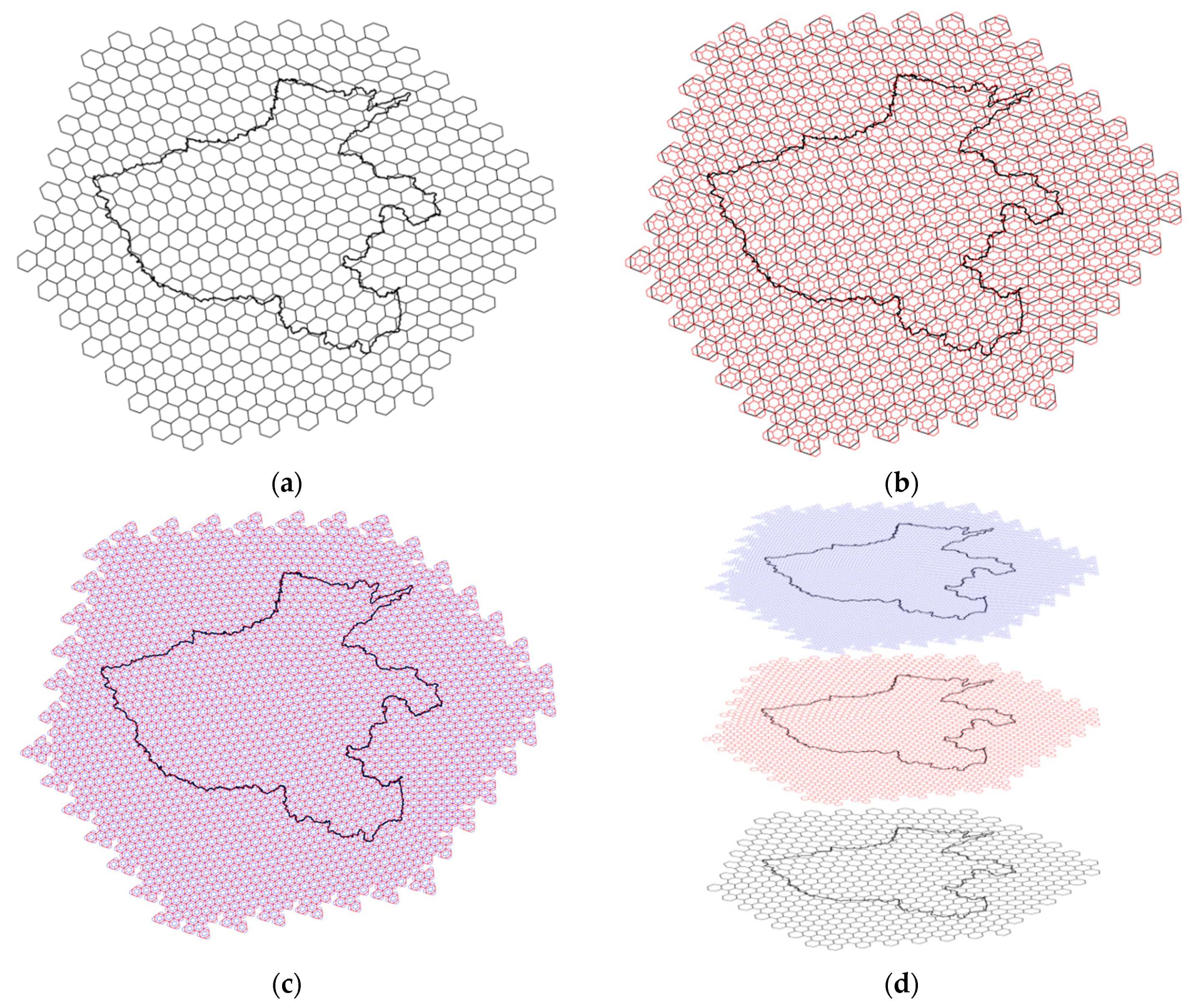
Figure 8.
Hierarchical indexing algorithm and pyramid model: (a) the indexing result of level 10 grids (initial resolution); (b) indexing from grid levels 10 to 11; (c) indexing from levels 11 to 12; and (d) the pyramid model of the hierarchical index algorithm.
Figure 8.
Hierarchical indexing algorithm and pyramid model: (a) the indexing result of level 10 grids (initial resolution); (b) indexing from grid levels 10 to 11; (c) indexing from levels 11 to 12; and (d) the pyramid model of the hierarchical index algorithm.

Figure 9.
Vegetation coverage classification in some provinces and cities in China.

Figure 10.
Schematic diagram of the DGGRID indexing algorithm.

Figure 11.
Efficiency comparison line charts for single-level indexing: (a) absolute value and (b) ratio.
Figure 11.
Efficiency comparison line charts for single-level indexing: (a) absolute value and (b) ratio.

Figure 12.
Efficiency comparison line chart for hierarchical indexing: (a) absolute value and (b) ratio.
Figure 12.
Efficiency comparison line chart for hierarchical indexing: (a) absolute value and (b) ratio.

Figure 13.
Visualization results for the indexing algorithm proposed in this paper: (a) global viewpoint and (b) local viewpoint.
Figure 13.
Visualization results for the indexing algorithm proposed in this paper: (a) global viewpoint and (b) local viewpoint.

Figure 14.
Visualization results for the bike-sharing data from Dongcheng district in Beijing using the indexing algorithm proposed in this paper: (a) from 8:00 to 9:00, where areas from A to E are Ditan park, the Russian Embassy, Beijing railway station, Temple of Heaven Park, and Longtan Park, respectively; (b) from 17:00 to 18:00; and (c) from 20:00 to 21:00.


Table 1.
Results of the single-level indexing comparison experiment.
| Level | DGGRID | The Proposed Algorithm | Efficiency Ratio | ||||
|---|---|---|---|---|---|---|---|
| Cells | Time (ms) | Efficiency (cells/ms) | Cells | Time (ms) | Efficiency (cells/ms) | ||
| 7 | 960 | 0.0808 | 11,881.188 | 676 | 0.0183 | 36,799.129 | 3.10 |
| 8 | 3534 | 0.3017 | 11,713.622 | 2524 | 0.0713 | 35,399.719 | 3.02 |
| 9 | 14,022 | 1.1721 | 11,963.143 | 10,444 | 0.3531 | 29,578.023 | 2.47 |
| 10 | 55,370 | 4.6023 | 12,030.941 | 39,676 | 1.5535 | 25,539.748 | 2.12 |
| 11 | 220,050 | 18.2345 | 12,067.784 | 154,588 | 7.1138 | 21,730.721 | 1.80 |
| 12 | 880,277 | 73.1306 | 12,037.054 | 621,076 | 32.5028 | 19,108.384 | 1.59 |
Table 2.
Results of the hierarchical indexing efficiency comparison experiment.
| Level | DGGRID | The Proposed Algorithm | Efficiency Ratio | ||||
|---|---|---|---|---|---|---|---|
| Cells | Time (ms) | Efficiency (cells/ms) | Cells | Time (ms) | Efficiency (cells/ms) | ||
| 8→9 | 13,899 | 3.2014 | 4341.538 | 10,096 | 0.0165 | 611,878.787 | 140.94 |
| 9→10 | 55,615 | 7.2554 | 7665.325 | 40,384 | 0.0778 | 519,074.550 | 67.72 |
| 10→11 | 220,539 | 20.4784 | 10,769.347 | 161,536 | 0.3125 | 516,915.200 | 48.00 |
| 11→12 | 878,323 | 74.2415 | 11,830.620 | 646,144 | 1.2279 | 516,218.747 | 43.63 |
| 12→13 | 3,517,353 | 293.9663 | 11,965.157 | 2,584,567 | 5.6475 | 457,647.985 | 38.25 |
© 2020 by the authors. Licensee MDPI, Basel, Switzerland. This article is an open access article distributed under the terms and conditions of the Creative Commons Attribution (CC BY) license (http://creativecommons.org/licenses/by/4.0/).
Share and Cite
MDPI and ACS Style
Zhou, J.; Ben, J.; Wang, R.; Zheng, M.; Du, L. Lattice Quad-Tree Indexing Algorithm for a Hexagonal Discrete Global Grid System. ISPRS Int. J. Geo-Inf. 2020, 9, 83. https://0-doi-org.brum.beds.ac.uk/10.3390/ijgi9020083
AMA Style
Zhou J, Ben J, Wang R, Zheng M, Du L. Lattice Quad-Tree Indexing Algorithm for a Hexagonal Discrete Global Grid System. ISPRS International Journal of Geo-Information. 2020; 9(2):83. https://0-doi-org.brum.beds.ac.uk/10.3390/ijgi9020083
Chicago/Turabian StyleZhou, Jianbin, Jin Ben, Rui Wang, Mingyang Zheng, and Lingyu Du. 2020. "Lattice Quad-Tree Indexing Algorithm for a Hexagonal Discrete Global Grid System" ISPRS International Journal of Geo-Information 9, no. 2: 83. https://0-doi-org.brum.beds.ac.uk/10.3390/ijgi9020083
Note that from the first issue of 2016, this journal uses article numbers instead of page numbers. See further details here.