Towards Detecting Building Facades with Graffiti Artwork Based on Street View Images


1
Institute of Geography, Heidelberg University, 69117 Heidelberg, Germany
2
Metropolregion Rhein-Neckar, 68161 Mannheim, Germany
*
Author to whom correspondence should be addressed.
†
These authors contributed equally to this work.
ISPRS Int. J. Geo-Inf. 2020, 9(2), 98; https://0-doi-org.brum.beds.ac.uk/10.3390/ijgi9020098
Submission received: 29 November 2019
/
Revised: 16 January 2020
/
Accepted: 27 January 2020
/
Published: 4 February 2020
Abstract
:As a recognized type of art, graffiti is a cultural asset and an important aspect of a city’s aesthetics. As such, graffiti is associated with social and commercial vibrancy and is known to attract tourists. However, positional uncertainty and incompleteness are current issues of open geo-datasets containing graffiti data. In this paper, we present an approach towards detecting building facades with graffiti artwork based on the automatic interpretation of images from Google Street View (GSV). It starts with the identification of geo-tagged photos of graffiti artwork posted on the photo sharing media Flickr. GSV images are then extracted from the surroundings of these photos and interpreted by a customized, i.e., transfer learned, convolutional neural network. The compass heading of the GSV images classified as containing graffiti artwork and the possible positions of their acquisition are considered for scoring building facades according to their potential of containing the artwork observable in the GSV images. More than 36,000 GSV images and 5000 facades from buildings represented in OpenStreetMap were processed and evaluated. Precision and recall rates were computed for different facade score thresholds. False-positive errors are caused mostly by advertisements and scribblings on the building facades as well as by movable objects containing graffiti artwork and obstructing the facades. However, considering higher scores as threshold for detecting facades containing graffiti leads to the perfect precision rate. Our approach can be applied for identifying previously unmapped graffiti artwork and for assisting map contributors interested in the topic. Furthermore, researchers interested on the spatial correlations between graffiti artwork and socio-economic factors can profit from our open-access code and results.
1. Introduction
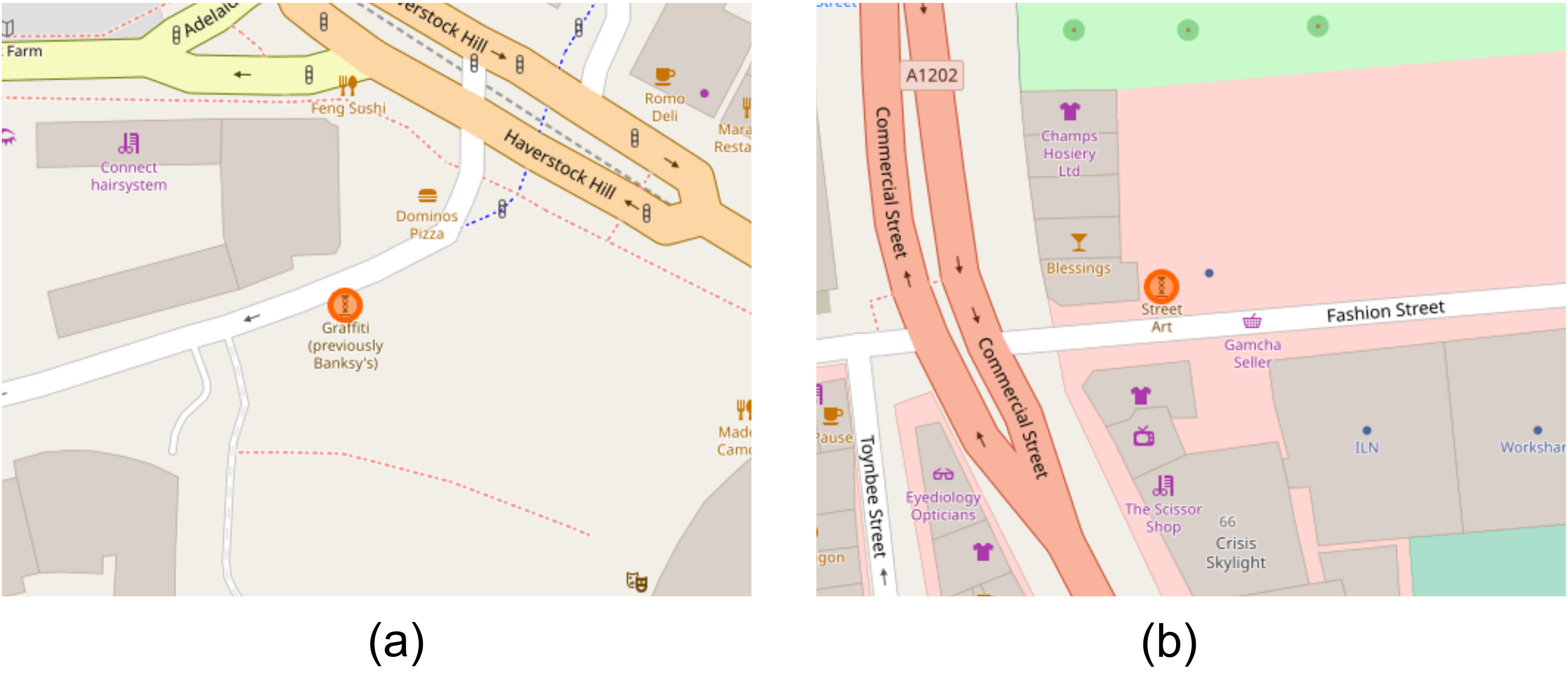
As a category of street art, graffiti makes use of the city’s walls, roofs and pavements as its canvas. It brings life and color to the city at the same time it raises questions and protests. Secluded to ghettos and seen as the work of vandals in the past, graffiti has now the status of genuine art and is thus recognized as a relevant expression of creativity, diversity and freedom [1,2]. Because of that, graffiti artworks are spatially correlated with commercial and social vibrancy and are associated with urban tourism and revitalization dynamics [3,4,5,6]. Despite the profusion of blogs, websites and books devoted to displaying and discussing graffiti artists and artworks, graffiti enthusiasts and urban planners frequently lack a reliable source of data on the exact location of graffiti works in a city. Graffiti is rarely mapped by municipal authorities and collectively kept platforms and commercial smartphone apps such as StreetArtMap, Positive Propaganda, Geo Street Art and Street Art Cities generally do not provide access (at least not free of cost) to their geo-referenced data. The Volunteered Geographic Information platform OpenStreetMap (OSM) [7], on the other hand, provides open access to contributed geo-referenced data on street art. However, OSM is still largely incomplete regarding graffiti artworks. The OSM Wiki website [8] advises contributors to tag graffiti as ‘tourism=artwork’ AND ‘artwork_type=streetart’ OR ‘artwork_type=street_art’ OR ‘artwork_type=mural’ OR ‘artwork_type=stencil’ OR ‘artwork_type=graffiti’. As shown in Table 1, a query on Tag Info [9] returned only modest numbers of these tags for the whole world as well as for the Greater London Area, one of the urban areas known for its profusion of street art works and street art-related tourism [4]. Through a careful manual inspection, we found out that OSM contributors frequently tag street art and graffiti features in London as ‘name=Street Art’, but a query with these tags only returned 74 features. Another issue of graffiti artwork data in OSM is that it is usually represented as nodes, i.e., as points in space, thus only indicating the approximate location of the artwork. See examples from Figure 1. Although this is not a problem for most map use purposes, applications like generating street art walking routes and the analysis of correlations between graffiti paintings and building characteristics (e.g., use, geometry, visibility) require knowing on which specific facades graffiti artworks are painted.
Although graffiti artists usually do not seek fame, they want their works to be appreciated and communicated with visitors and the local community [6]. Making graffiti artworks more visible and accessible by mapping them moves us closer to this goal, thus strengthening the sense-making dynamic of this type of art. Furthermore, this helps to increase graffiti’s geographic and economic values. In this work, we propose a workflow for locating building facades with graffiti artwork. It starts by identifying the approximate location of graffiti artworks based on geo-tagged photographs from the image hosting service and social media Flickr. Following, based on Google Street View [10] images, automatic image interpretation, and OSM street and building data, the building facades in the surroundings of the approximate graffiti locations are inspected on whether they contain graffiti art or not.
The remainder of this paper is structured as follows. In Section 2, we briefly review related works on the processing of street view images for the characterization of urban spaces. Section 3 describes in detail the methodological steps undertaken in this work. Section 4 describes the experiment performed for testing our approach. In Section 5 we present and discuss the obtained results. A conclusive discussion and outlook is provided in Section 6.
2. Related Work
In this section, a brief overview is given on works leveraging different urban applications through the processing of street view images. Being the first and best known source of this type of data, Google Street View (GSV) images have been used in the majority of these works. The main reason for this might be that GSV images are available for many cities in the world and can be, up to a certain amount, obtained free-of-cost through the Street View Static API [11].
Being an important aspect of the visual pleasantness and climatic comfort of urban landscapes, street-level greenery is frequently the focus of analysis of these studies. In one of the earliest efforts in this direction, Li et al. [12] proposed a modified green view index computed based on green areas extracted from GSV through simple rule- and pixel-based image processing operations. They suggest that objective measurements of street-level greenery can be obtained in this way. Similarly, Seiferling et al. [13] applied image segmentation and classification techniques on GSV images for quantifying the tree canopy cover at the street-level. Not always though street-level greenery is analyzed automatically. Berland et al. [14] conducted an experiment in which human analysts visually interpreted GSV images and estimated the number, species, and diameter at breast height of street trees. Their results suggest that such virtual survey may be conducted for efficiently obtaining and updating urban tree datasets. Besides GSV, Tencent [15] is also an important source of street view images for urban greenery analysis. Zhang and Dong [16] used street view imagery from Tencent and the SegNet [17] neural network tool for quantifying the street-visible greenness of residential neighbourhoods. They observed that street-visible greenness is one of the variables that significantly correlates with housing prices. Tang and Long [18] also used SegNet and Tencent street view images for measuring the visual quality of streets based on the morphological features of greenery, openness and enclosure. They discuss how these features correlate with street activity and with the citizens perception of environmental and social pleasantness.
Street view images have also been used for describing urban canopy parameters. Sky view factor is an expressive metric used for describing the morphology of urban canyons and can be effectively estimated with street view images. Cheng et al. [19] acquired Tencent street view images with angles corresponding to the human visual field. They then applied standard image processing procedures for extracting sky and green features. The sky openness and greenness view indexes they propose aim to facilitate the assessment of the human visual perception of urban landscapes. Middel et al. [20] converted 90 images from GSV into hemispheric views and used them to compute the sky view factor of almost 16 million GSV locations. Their approach rely on the binary sky/non-sky segmentation of the hemispheric images. Their sky view factor estimations were compared to those generated based on the results produced by Middel et al. [21], in whose work 90 GSV images were segmented into six classes including sky, trees and buildings using a deep learning framework. Zeng et al. [22] presented an approach developed in Python with the OpenCV library for estimating the sky view factor of large amounts of Baidu Street View images.
Street greenery and the sky view factor can be considered together for analyzing the thermal comfort of pedestrians. Li et al. [23] estimated the shading effect of street trees by subtracting the sky view factor estimations computed from GSV panorama images and from a building height model. Richards et al. [24] quantified the proportion of tree canopy coverage of streets based on GSV hemispherical images and image classification techniques. With this data they estimated the proportion of annual solar radiation that the tree canopies block. Gong et al. [25] proposed an approach for computing the sky, tree and building view factors of urban canyons by detecting these features in GSV images classified with a deep-learning algorithm. They verified their estimates with hemispheric photographs from fields surveys and reported a very high agreement of the estimations.
Other researches have focused on more social topics based on street view image data. Aiming to contribute to the research on finding patterns of walkability in a city, Yin et al. [26] attempted to extract pedestrian count data from GSV images using the ACF feature detection algorithm [27]. Kang et al. [28] proposed a framework for classifying the functionality of individual building footprints by classifying GSV images of their facades as well as remote sensing images of their rooftops using a convolutional neural network model. They also provide a large dataset of street view images of the facades of eight building types, which can be used for training other models.
These works demonstrate that street view images are a relevant type of data for estimating parameters that play an important role in the street’s environmental conditions and perception by residents and pedestrians. As such, they can effectively contribute to urban planning and policy-making. However, street view images have only been scarcely applied in studies related to the streets aesthetics [18,29,30]. In this work, we take a step in this direction and demonstrate the potential of this type of data for supporting the mapping of graffiti artworks in a city. The next section describes the methods we applied to this aim.
3. Methods
The methodology applied in this work is comprised of three main parts, namely, (1) finding the approximate location of graffiti artworks, (2) extracting and interpreting GSV images from the surroundings of these approximate locations, and (3) detecting the building facades depicted in the GSV images interpreted as containing graffiti artwork.
3.1. Finding the Approximate Locations of Graffiti Artworks
This step leads to a significant reduction of the area where graffiti artworks will be searched. Processing all GSV images from a whole city would be too time-consuming and computationally demanding. The approximate location of graffiti artworks was extracted based on geo-tagged photographs from Flickr, a photo hosting and sharing social media. More specifically, we first analyzed how Flickr users semantically tag graffiti photos and then used this folksonomy for measuring the relatedness of geo-tagged Flickr photos to the topic of ‘graffiti’. In the next two sections we present how these two steps were undertaken.
3.1.1. Capturing the Folksonomy of Graffiti Artwork in Flickr
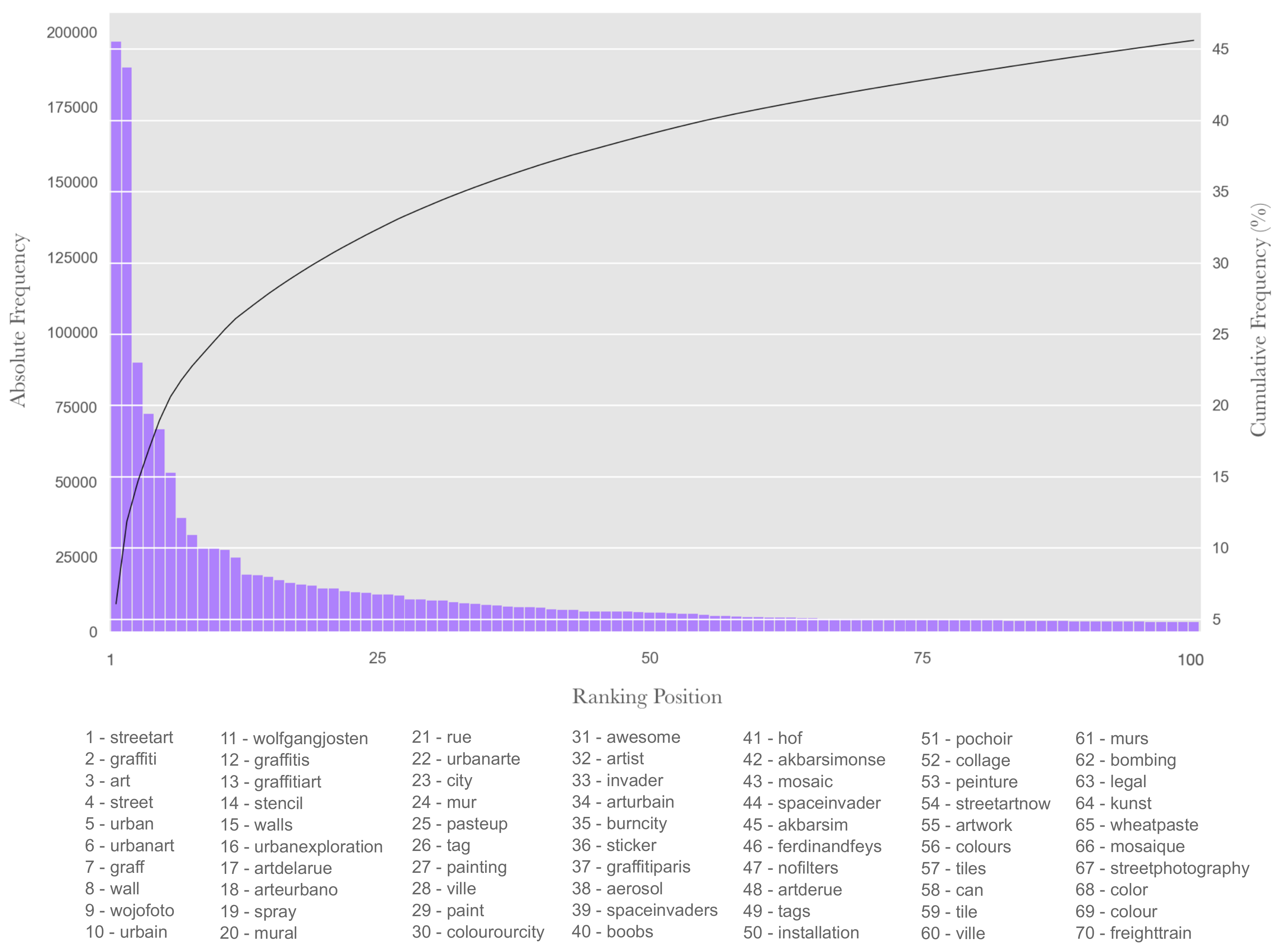
An important step of our methodology is the identification of geo-tagged Flickr photos of graffiti content. We identified such photos based on the folksonomy, i.e., the collective tagging, of graffiti in Flickr. For capturing this folksonomy, photos from representative Flickr groups related to the topic of graffiti and street art were sampled. Approximately 301,000 photos were randomly sampled from the groups presented in Table 2. The sampled photos contain in total about 3.2 million user-defined tags. The groups from Table 2 were chosen due to their large amount of members and posted photos as well as due to their high relatedness to the topics of graffiti and street art. After ranking in descending order of frequency about 109,000 different user-defined tags from these sampled photos, we manually excluded location-related tags (e.g., ‘London’, ‘france graffiti’, etc.) appearing in the first 200 positions of the frequency rank. Also, all tags with less than three or more than twenty characters were automatically excluded from the entire ranking. Figure 2 shows the distribution of the 100 most frequent tags from the sampled photos. It can be seen that in a ranking of almost 109,000 entries, the first five have a significantly higher frequency than the ones lower in the rank. Not surprisingly, these most frequent tags are ‘streetart’, ‘graffiti’, ‘art’, ‘street’ and ‘urban’. Also, we observed that the tags below the 100th position in the ranking have very low frequency percentages in the folksonomy. This is demonstrated by the cumulative frequency distribution of the one-hundred most frequent tags also presented in Figure 2. It can be seen that the one-hundred most frequent tags cover about 45% of all user-defined tags from the sample photos and that the first five tags cover about 20% of all photo tags.
3.1.2. Measuring the Relatedness of Geo-tagged Flickr Photos to Graffiti Artwork
After capturing the folksonomy of graffiti photos from Flickr, the next step was the quantification of the relatedness to graffiti of geo-tagged Flickr photos in general, i.e., regardless of they being in a Flickr group or not. We estimated this relatedness based on the following metric:
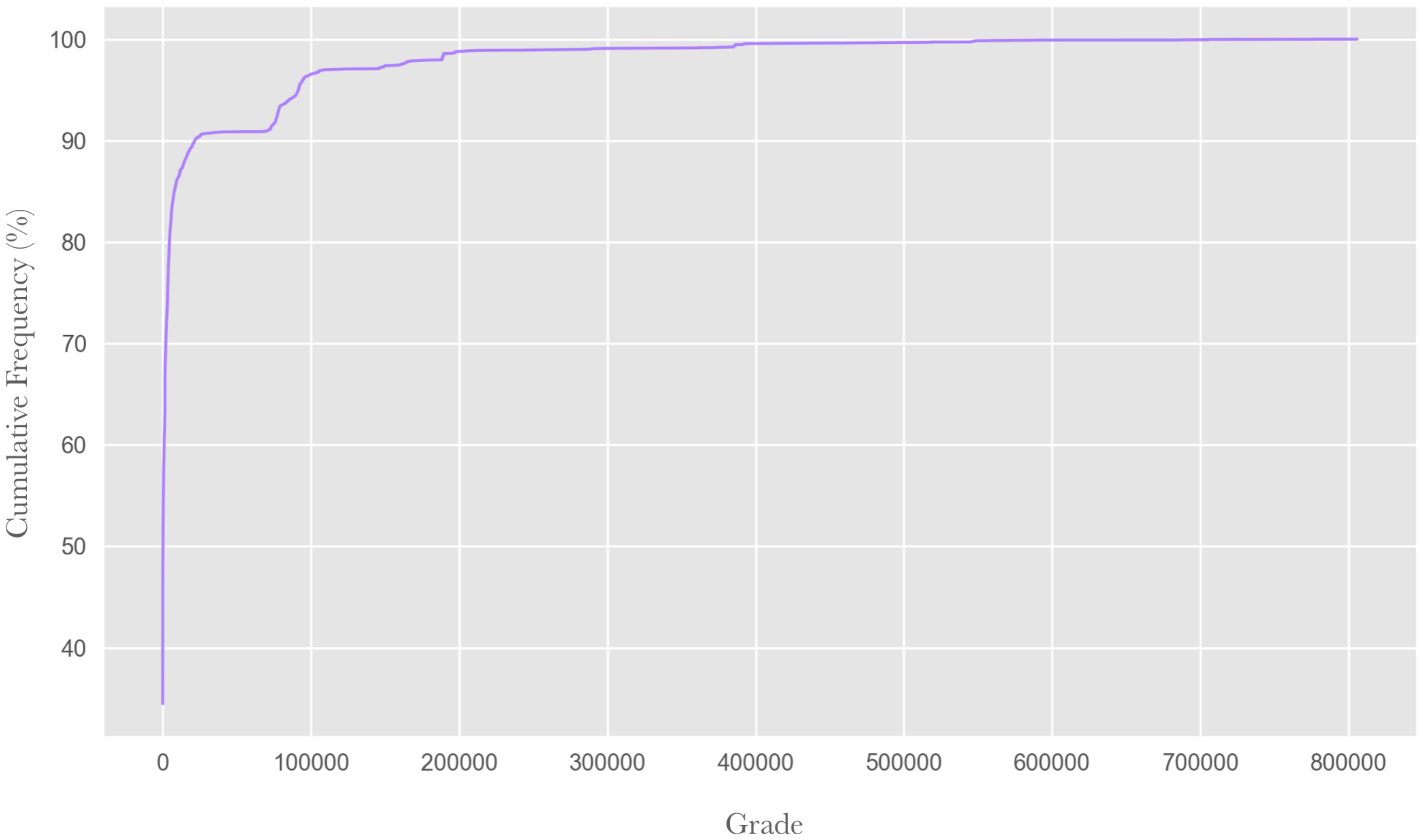
where denotes the relatedness of geo-tagged photo i to graffiti, t denotes each of the n tags from photo i, and denotes the total frequency of this tag in the sampled photos. Figure 3 shows the cumulative frequency distribution of the relatedness to graffiti of all 191,234 geo-tagged Flickr photos from the Greater London Area. It can be observed that about 90% of these photos have relative low relatedness to graffiti. Also, the function being close to a horizontal line above the 95% mark indicates that a relatively low amount of photos has very high relatedness to graffiti. We observed that all the 100 photos with the highest measured relatedness are undoubtedly of graffiti content. We also observed that 37% of the geo-tagged photos from the test-site with relatedness to graffiti above the 90th percentile (n = 8538) are not in any Flickr group. The remaining 63% of the geo-tagged photos are in 6920 different groups (many photos are in several groups). We noticed that the 10% most frequent of these groups are not related to street-art nor to graffiti. This lets us assume that the percentage of geo-tagged photos above the 90th percentile of graffiti relatedness and not belonging to any graffiti or street art group is probably considerably higher than 37%. If we had limited our search to geo-tagged photos posted in graffiti-related groups, we would have missed a significant number of geo-tagged photos that are very likely of graffiti artwork content.
3.2. Extracting GSV Images from Relevant Building Facades
After identifying geo-tagged Flickr photos with high relatedness to graffiti, we focused on identifying the actual building facades on which graffiti artworks are painted. This is not a trivial task as geo-tagged photos from Flickr have an average positional error of 58.5 m [31]. Therefore, in theory, every facade in a radius of approximately 60 m around the photos’ coordinates may contain the artwork depicted on the photo (assuming it has not been erased). Thus, a bounding-box of equal sides of 120 m was centered on the position of each geo-tagged Flickr photo with high relatedness to graffiti. Following, all GSV image acquisition locations inside the bounding-box were extracted. These are discrete points in space from which the camera onboard the GSV vehicle acquires images in all directions. For each GSV image acquisition point, twelve images were collected with compass headings (h) ranging from 0 to 330, thus
The field-of-view of each image acquisition was kept as its default value, namely, 90. The GSV API requires the definition of these three parameters, i.e., the geographic coordinates, the compass heading and the image’s field-of-view, for providing images to the user [10]. By means of an artificial neural network (see Section 3.3), all images from inside a bounding-box were interpreted as containing graffiti artwork or not, where n represents the amount of GSV image acquisition locations inside the bounding-box. If according to the neural network interpreter, the probability of the GSV image from bounding-box b, location l, and heading h is above or equal 0.99, these three parameters were saved in our database. Note that a single GSV point may have multiple graffiti-containing images of different compass headings.
3.3. Interpreting the GSV Images
In this work, we aimed to identify building facades containing graffiti artwork based on machine learning interpretation of GSV images. For that, as mentioned, an artificial neural network was trained, tested, and applied. As it would have been excessively time-consuming to implement and train such a network from scratch, we resorted to a transfer learning solution and built upon an existing and pre-trained model, namely, the VGG16 convolutional neural network (CNN) developed by Simonyan and Zisserman [32]. CNNs are a class of deep neural networks that have been successfully applied for social media image interpretation [33,34,35] as well as in computer vision [36,37] and remote sensing applications [38,39]. The VGG16 network was trained and tested based on ImageNet, a image dataset of over 14 million pictures of about 1000 classes [40]. As graffiti artwork is not one of these classes, and in order to make the model applicable to our specific image interpretation problem, we instantiated only the convolutional blocks of the VGG16 network. This truncated model can be considered as a feature extractor to which the GSV images were input. Next, we created a customized neural network trained based on the features extracted at the last pooling layer of the truncated VGG16 model. The features output at this layer in format 7 × 7 × 512 were flattened to the 25,088 × 1 shape. The customized part of the CNN is comprised of three fully connected layers, where in each layer, as a recommended measure for preventing over-fitting [41], a dropout with p = 0.5 was applied.
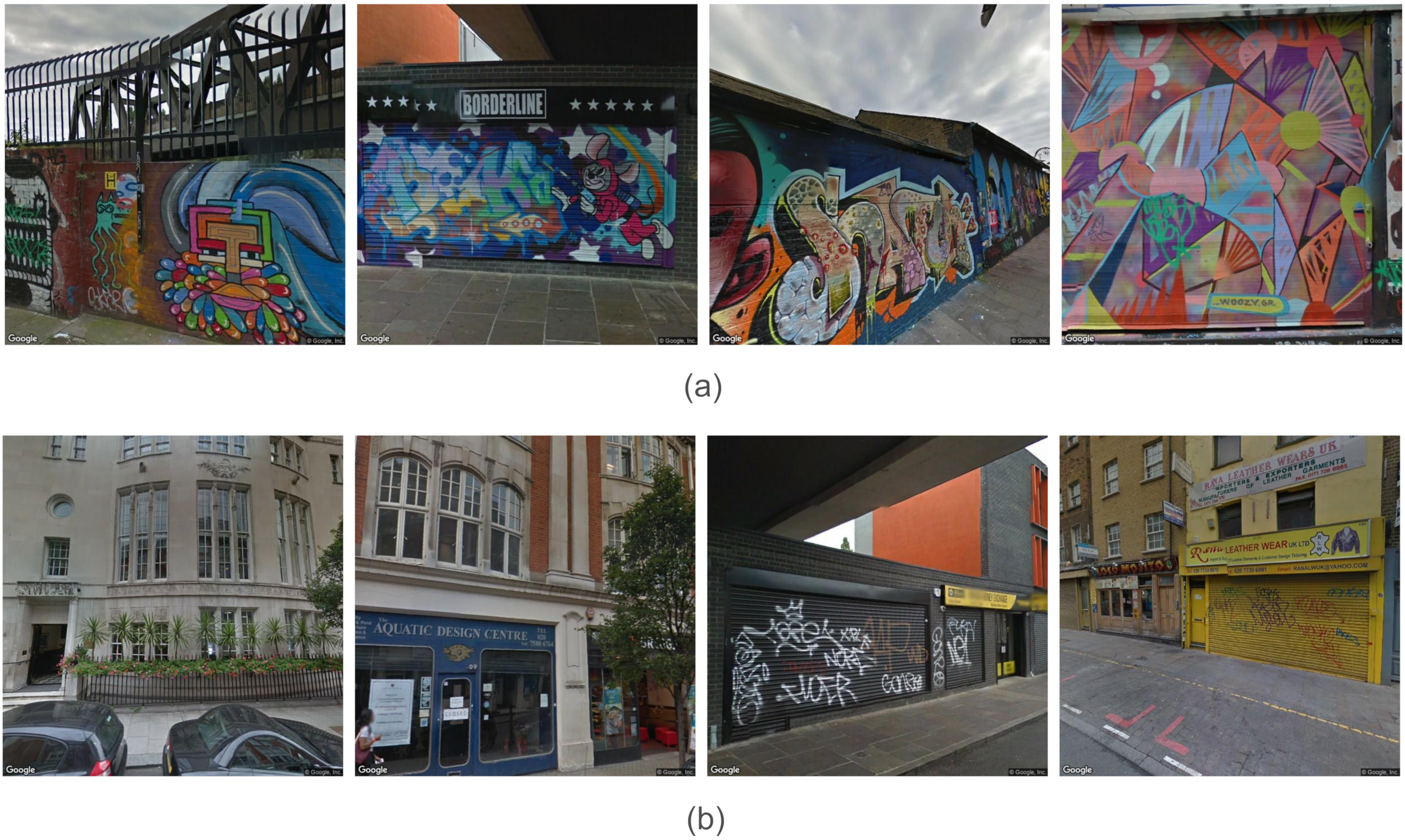
The complete CNN was then trained for 100 epochs on 260 images per class using 8 samples per batch. Figure 4 shows four samples of each of the two considered classes, i.e., ‘graffiti’ and ‘not graffiti’. The GSV sample images were all collected from the Greater London Area (United Kingdom), the study-area of this work. The samples from the ‘not graffiti’ class included randomly selected facades that do not contain graffiti as well as GSV images of facades which could potentially cause false-positive misclassifications, such as advertisement signs and “scribblings”. Binary Cross-Entropy was used as the loss function, which was optimized with the AdaGrad algorithm [42] with a learning rate of 0.001. Table 3 shows the complete structure of the image interpretation model and Table 4 presents the confusion matrix obtained when testing the model with 50 samples from each class. It can be seen that an overall accuracy of 93% and a Kappa index [43] of 0.86 were obtained. Aiming to enable the reproducibility of our results as well as the model’s application in other studies and analyses, our full CNN is made available online at https://github.com/le0x99/SA_classifier.
3.4. Detecting the Building Facades Containing Graffiti Artwork
After extracting the acquisition location and compass heading of all GSV images that, according to the CNN presented above, contain graffiti artwork, the next step of our approach was the detection of the actual building facades in which these graffiti artworks are painted. In this section, we present the strategy applied to this goal.
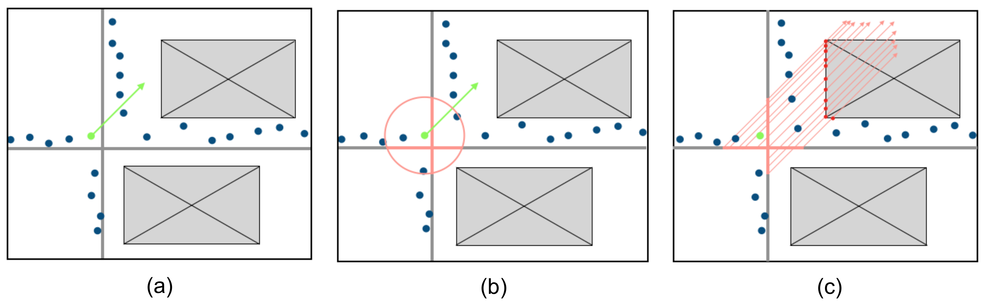
Due to the positional uncertainty of the GSV image acquisition locations, a 5 m radius was set around each of the locations in which at least one of its twelve images, acquired in different compass headings (i.e., h in Equation (2)), graffiti artwork was detected by the CNN model. Following, all street segments intersecting this radius were extracted. Lastly, parallel lines were projected from these intersecting street segments in the heading direction(s) of the graffiti-containing image(s) and the facade(s) intersected by these projected lines were extracted as candidates of containing graffiti. This process is illustrated in Figure 5.
Although there is uncertainty regarding the true position of the GSV image acquisition, it was assumed that the true position is on the street, as the GSV camera is set up on the top of a car. Both the building facades as well as the street segments intersecting the radius were obtained from OSM. It should be noted that the OSM building segments visible from the streets (defined as “ways”) are not guaranteed to correspond to real building boundaries. Either way, we counted the number of points of intersection between each OSM facade and the parallel projection lines. These points are depicted in red in Figure 5c. Facades with more points of intersection are in general more likely to contain graffiti artwork. However, because the length of the street segments inside the radius are variable, the intersection points should account with different weights to the potential that the facade contains graffiti. Therefore, for each street segment inside the 5 m radius, we projected exactly nine parallel lines in the compass heading of the image(s) containing graffiti artwork. The points of intersection between these lines and the OSM facade segment will account to the overall score of that facade having graffiti by a weight w given by , where l represents the length of the street segment inside the radius from which the projection line intersecting the facade has its origin. The overall potential of a OSM facade containing graffiti artwork equals the sum of the weights of all points of intersection between that facade and the projection line. This potential was computed for every OSM building segment visible from the streets and spatially intersecting the 120m-side bounding-box centered on the Flickr geo-tagged photo with high relatedness to graffiti artwork (see Equation (1)).
4. Experiment
For testing the approach presented above, the Greater London Area (United Kingdom) was chosen as test-site, whose perimeter can be visualized at https://www.openstreetmap.org/relation/175342#map=11/51.4898/-0.0882. The reason for choosing London as test-site was threefold: (1) this city is worldwide known as profuse in graffiti artworks. In particular, parts of town such as Brick Lane, Shoreditch and Hackney Wick are specially famous for the abundance of graffiti; (2) photos of graffiti posted on related Flickr groups are often times taken in London as well as in Paris and Berlin; and (3) GSV images of London are up-to-date and available for the whole city.
A total of 191,234 geo-tagged Flickr photos were collected from the study-area and evaluated according to their relatedness to graffiti artwork. These photos were taken between June 1st of 2014 and January 1st of 2018. All photos have the maximum Flickr geo-location accuracy parameter of 16. As described above, the initial input to our approach for detecting building facades containing graffiti artwork are the coordinates of a Flickr photo with high relatedness to graffiti. The output of our approach is a score computed for each OSM building facade inside the bounding-box centered on a Flickr photo, which expresses the potential that the facade contains graffiti. As it is not feasible to process and manually check each facade within the 120 meter-side bounding box centered on each of these almost 200,000 Flickr geo-tagged photos, for the purpose of testing our approach, we limited our analyses to the 40 Flickr photos with highest relatedness to graffiti. The total amount of OSM facades inside these 40 bounding-boxes is of 5613 and the total amount of GSV images interpreted by our customized CNN model is 36,804.
5. Results
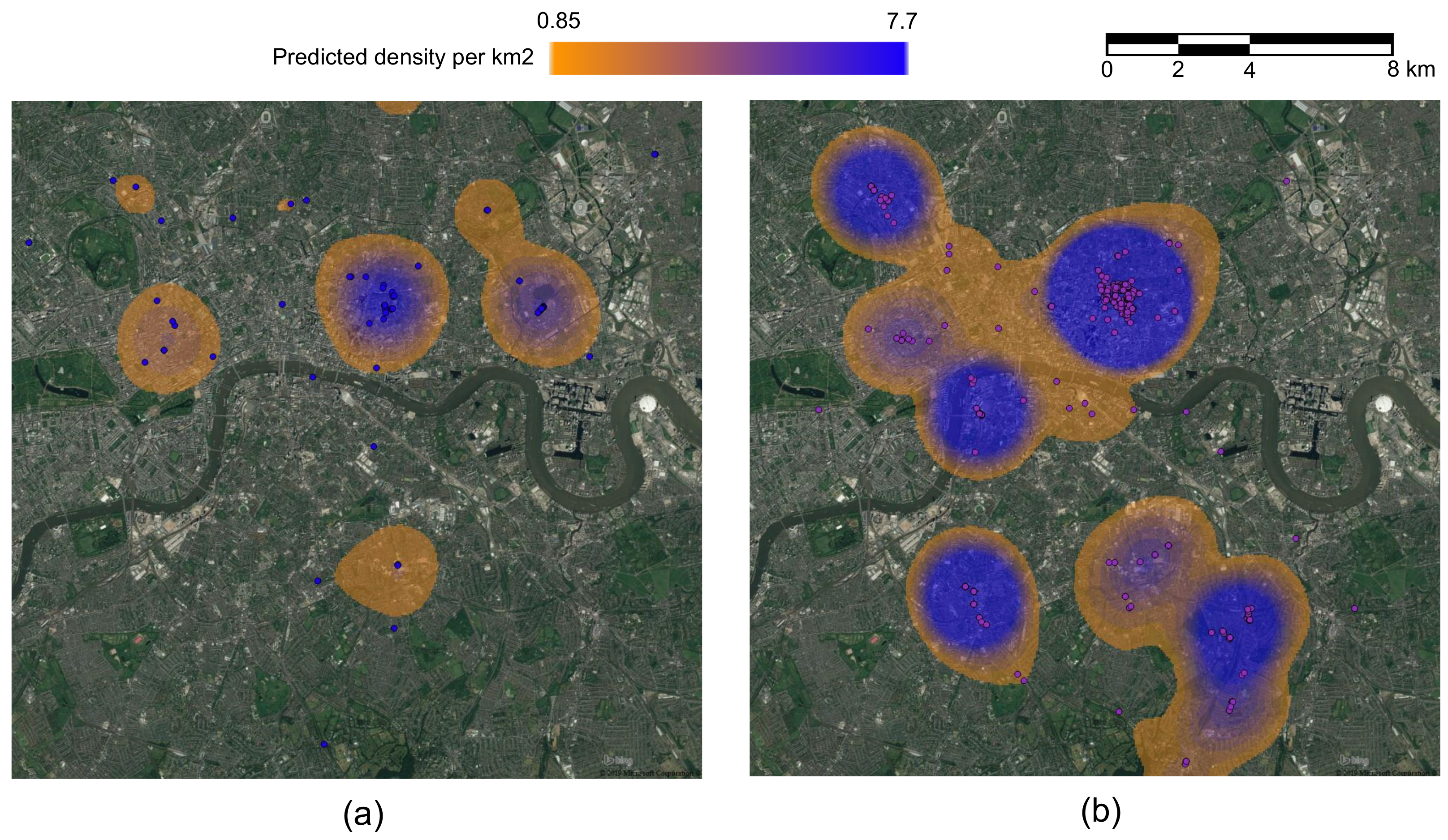
In the introduction part of this paper, we argued that, according to how the OSM-Wiki page advises contributors to tag graffiti artworks, to a query performed in TagInfo, and to our empirical knowledge of London, OSM is still incomplete regarding this type of information in this city. This is very likely the state of things in OSM in other less prominent cities as well. Figure 6a shows a kernel density map of the 87 OSM features containing the graffiti artwork-related tags (see Table 1) found in the central part of London. Figure 6b shows the same map for the 617 Flickr geo-tagged photos containing both the tags ‘street-art’ and ‘graffiti’. It can be seen that the number of potential graffiti artworks and their hot spots is considerably higher in Figure 6b than in Figure 6a, thus making the point that, as a dataset, Flickr is complementary to OSM and can indicate the areas where a more focused search of graffiti artwork should be undertaken with the aim of detecting the specific facades in which they are painted.
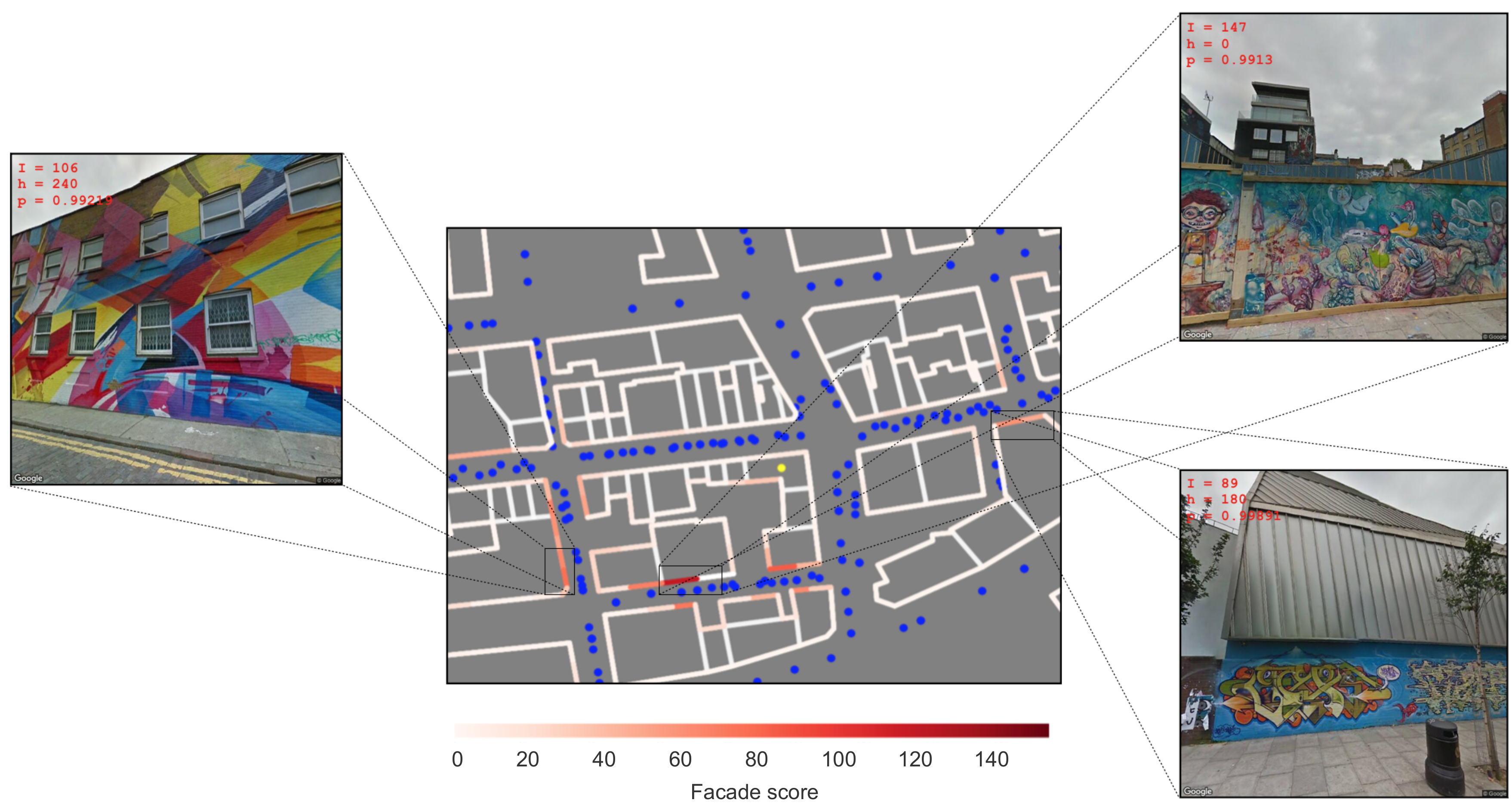
Among the 5613 OSM facades analysed in the bounding-boxes centered on the 40 geo-tagged Flickr photos most related to graffiti artwork, 420 of them had at least one projection line intersecting them (see Figure 5). Aiming to facilitate the manual evaluation of our approach as well as to potentially support other analyses by other researchers, we developed and made accessible computational code written in Python for the visualization of the facade scores regarding their potential of containing graffiti artwork. Figure 7 shows an example of the cartographic outcome of our approach, namely, a 120 m-side bounding-box centered in the geo-tagged graffiti-related Flickr photo (represented by a yellow dot), the building footprints from OSM, and the facades coloured according to their score of potential of containing graffiti. The figure also shows that, in this case, dark-red coloured facades truly contain graffiti. This is, by the way, another positive effect of inspecting every facade in each bounding-box, i.e., the detection of more facades with graffiti than what is photographed and posted in Flickr. Together with the data collected and produced during this research and the CNN used for interpreting the GSV images, the code for producing the visualization presented in Figure 7 can be accessed through the link https://github.com/le0x99/SA_classifier.
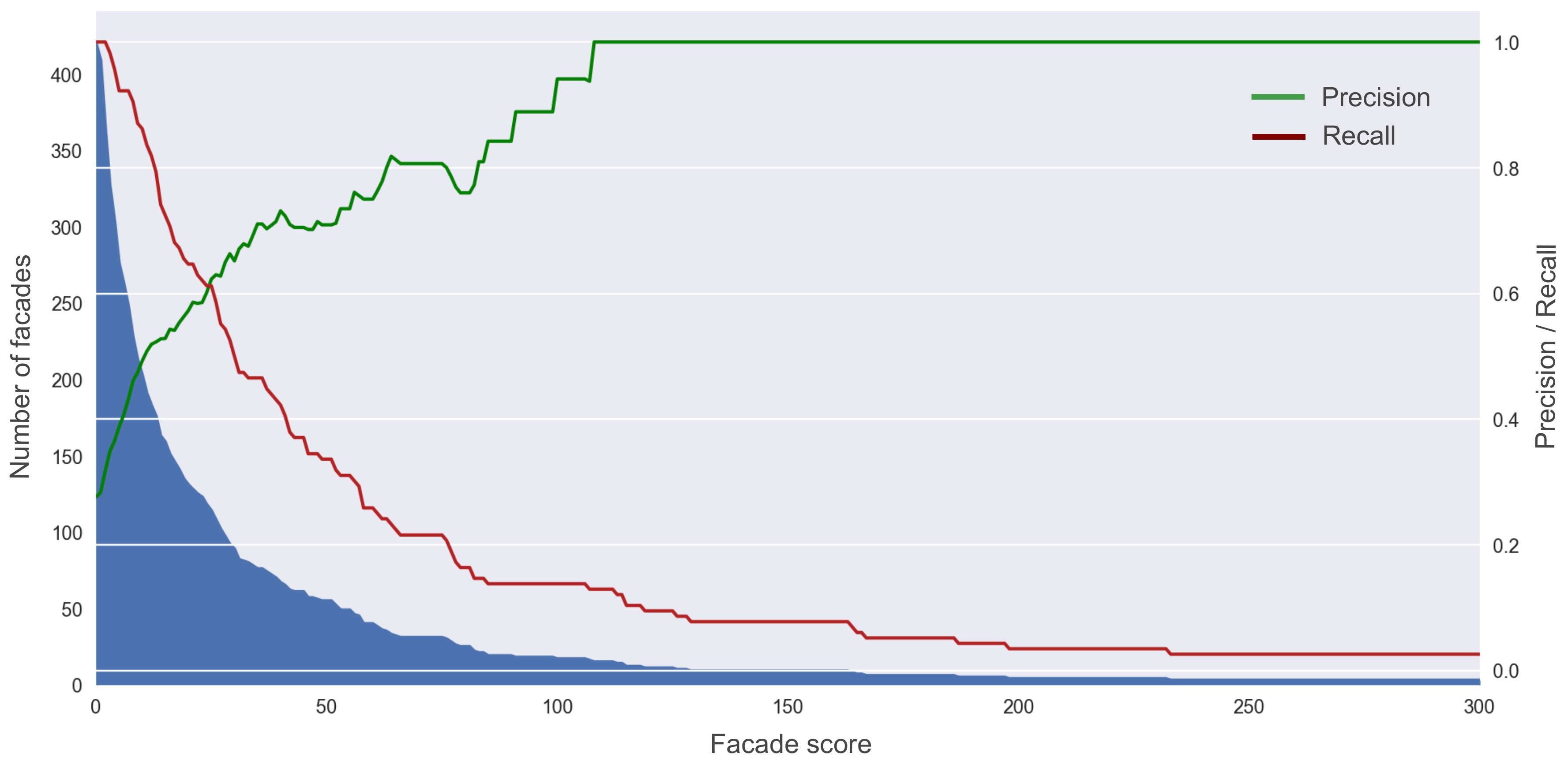
In Figure 8, the number of OSM facades (y axis in the left-hand side) with a score equal or larger than every value in the x axis of the graph is shown (in blue). As mentioned, the number of OSM facades with a score larger than zero is 420 for the 40 analyzed bounding-boxes. The green and red lines indicate respectively the precision and recall rates (y axis of the right-hand side) obtained when classifying as containing graffiti artwork all OSM facades with a minimum score of all values in the y axis range. Thus, for example, when considering a threshold score of 1, the recall rate is of 1.0, but the precision rate is of only 0.3. When considering a threshold score of 100, the recall rate is below 0.2, however the precision rate is above 0.8, and the number of detected OSM facades is of about 20. As much as we regret low recall rates and thus larger numbers of false-negative errors, it should be noted that maximizing the precision rate, i.e., eliminating all false-positive errors, is for the purpose of detecting previously unmapped graffiti artwork most important. A precision rate of 1.0 is achieved at the threshold score of 108, which leads to the correct detection of 15 OSM facades. None of these facades nor their respective building features have any graffiti-related OSM tag. Therefore, our results provide evidence that our approach can lead to the correct detection of OSM facades containing graffiti artwork if the score for classifying facades as such is set high. Although, as Figure 8 shows, many true-positive facades can be expected to occur, applying our graffiti detection approach to many locations indicated by the coordinates of Flickr photos with high relatedness to graffiti artwork will lead to the detection of many facades containing graffiti. Due to the excessively long time and energy taken to manually verify each facade, what involves identifying the corresponding facades in OSM and in the GSV images, we limited our analysis to 40 Flickr photos and in total 420 OSM facades.
Concerning the errors observable in the precision rate curve shown in green in Figure 9, these are of two types. The first refers to false-positive errors caused by misinterpretations by our customized CNN model. Besides specially colourful store facades such as the ones shown on the upper part of Figure 9, advertisements, posters and graffiti “vandalism” (shown in the middle part of Figure 9) are elements that were found to cause false-positive interpretations. These errors can be overcome to the extent that training the network with more and better samples in the sense of more representatively covering the full range of true-negative cases will lead to more accurate interpretations by the CNN. However, the subjectivity of where art begins and vandalism and dirty scribblings end will always pose a challenge to the evaluation of results.
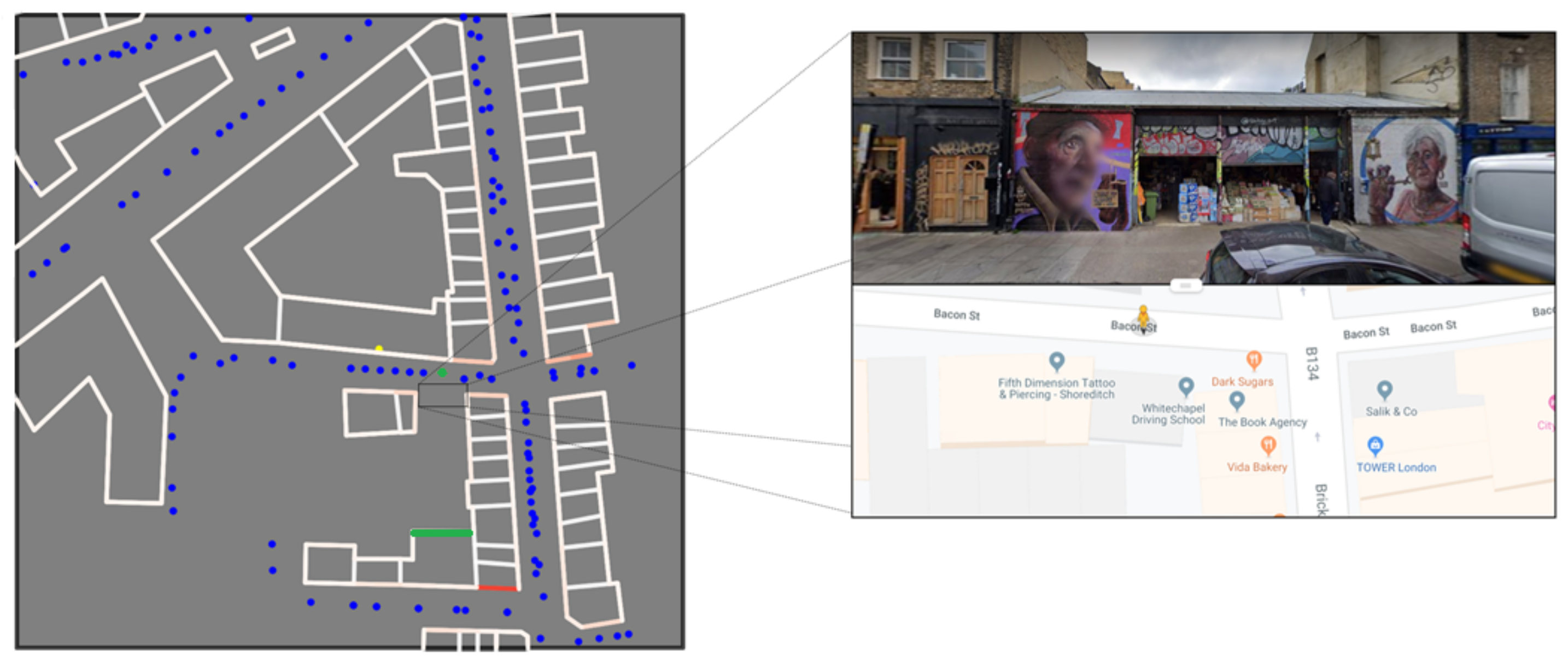
The other type of false-positive error relates to the fact that OSM and GSV are different datasets with different feature contents and a temporal mismatch. The lower part of Figure 9 shows trucks correctly interpreted as containing graffiti artwork. However, they cannot, as our approach automatically does, be associated to the building facades behind them. Another source of false-positive error is the temporal mismatch between the datasets. Figure 10 shows one of the 40 bounding-boxes considered in the evaluation. The green dot represents one of the GSV image acquisition points. The CNN model identified graffiti street art in the heading direction of 180. The corresponding image is shown on the right-hand side of the Figure 10. It was a correct interpretation as it does contain graffiti artwork. However, as this feature was not mapped at OSM at the time of writing this paper, the artwork was incorrectly associated to the building facade further south of it (highlighted in green).
6. Summary and Discussion
In this work, we presented an approach for first detecting the approximate location of graffiti artworks (with a geometrical uncertainty of 60 m) based on Flickr data, and then computing the potential of individual building facades around these locations containing graffiti artwork. Our analyses indicate that (1) OSM is still incomplete and geometrically imprecise regarding this type of data; (2) Flickr, despite its reduced use in recent years, is still a relevant source of data on the approximate spatial location of graffiti in the city; and (3) street-level imagery can support, position-wise, a more accurate detection of previously unmapped and not-posted graffiti artwork.
Adding to a number of works on the characterization and analysis of urban spaces based on the processing of street view images, we demonstrated the applicability of transfer machine learning image interpretation for identifying the presence of graffiti artwork on GSV images. Taking into consideration the compass heading of the GSV images in which the CNN identified graffiti, the positional uncertainty of the location of their acquisition, and based on OSM’s street and building features, we presented an approach for estimating the potential of specific OSM building facades having graffiti artwork.
Regarding our approach’s accuracy, the following aspects are probably the main ones potentially causing misclassifications. (1) Misclassifications caused by the adapted CNN: no classifier is perfect, specially when the object of interest is as complex as human-painted features embedded in complex environments such as urban areas. Besides, as mentioned, there is a fine line separating graffiti art from graffiti as vandalism and other forms of expression. It is reasonable to assume that increasing the number and diversity of training samples is expected to make the CNN perform even better, as is usually the case. (2) The possible positional disagreement between the GSV and OSM datasets: GIS scientists and practitioners known that working simultaneously with different geo-datasets often requires dealing with geometrical mismatches, which are usually not simple to model. We conceived and implemented a simple strategy for computing the potential that building facades contain graffiti. The strategy’s detection accuracy is however dependent on the positional uncertainty of the GSV image acquisition location and on the positional and geometric accuracy of the data set containing the buildings’ representations. (3) The temporal mismatch between the datasets: there is a time gap between the date the geo-tagged Flickr photos were taken and the date the GSV images were acquired. In cases the Flickr photo is outdated, i.e., taken from a no longer existing graffiti, our approach will look and not find any graffiti artwork in the GSV images. We should stress in this regard that graffiti artworks are frequently ephemeral, i.e., under constant change. Thus, often times the photographed artwork is not the same detected by the CNN model in the GSV images. Instead, it is frequently an updated or transformed version, or even a complete substitution of it. However, only rarely graffiti artworks are completely erased. If they are erased though and the GSV images are outdated, false-positive misclassifications will in reality occur. In case both the GSV images and Flickr photos are outdated, false-positive errors are expected to occur. In case only the GSV images are dated previously to the painting of graffiti, a false-negative error will occur. Another data-related aspect leading to errors is the one depicted in Figure 10, i.e., graffiti is detected in a building not yet mapped at OSM. This will lead to the assignment of a higher score to the facade located directly behind it. (4) Errors caused by obstructing objects: any object obstructing the facades, such as cars and trees may hamper the detection of graffiti, if it exists. Likewise, as shown in Figure 9, movable features containing graffiti and detected as such will lead to the false-positive assignment of graffiti to the OSM facade located behind those objects. (5) Errors emerging from the not adjusted GSV camera parameters: by better adjusting the fov and pitch parameters of the GSV image acquisition API, so as to focus more accurately on the building facades, the CNN classifier could deliver more accurate results. However, as stressed, the geometrics of the fov parameter is unfortunately not documented by GSV. Regarding the pitch parameter, a 3D city model is required if it is to make a difference in the exact focusing of the GSV images. In this work, however, we considered only 2D building representations obtained from OSM.
Some OSM features are already tagged with a link to a photograph or image of it posted on social media or available in other street view image sources, like Mapillary and OpenStreetCam. We share the opinion that associating street-level images to map features can leverage the use of the map for different purposes and enhance its interactivity. Although GSV is by far the street view image source with highest coverage (compared only to Tencent in some parts of the world), license issues hinder the linkage of GSV images to open geo-datasets like OSM [44]. Mapillary and OpenStreetCam, on the other hand, do not offer this legal impediment. However, this street view image sources presently cover mostly main roads of main cities only. Given the availability of street view imagery though, the up-scaling of our approach to larger areas and other cities of the world can only be hampered by constraints related to data processing resources. The automatic interpretation of large sets of images is possible given the present availability of multiple open-source/access CNNs training frameworks available online, such as TensorFlow, PyTorch, and Apache MXNet, to name a few. Options from the commercial world that are also effective but restrictive or cost-involving include Clarifai [45] and AWS from Amazon. It should be noted that, as mentioned, Flickr is considered in this work as a data source indicating relevant areas for a more detailed search of graffiti. In theory, however, the street view image interpretation and the assignment to building facades of a score representing their potential of containing graffiti artwork can be undertaken for whole parts of town or even the entire city.
In the context where location-based services are becoming more and more used tools for locals and tourists to know where to go, how to get there and what to experience in a city, mapping such important features of the city’s aesthetics as graffiti artworks is of high relevance. The approach we present in this paper is an effort for supporting the mapping of graffiti artworks based on automatic data analysis procedures. Making the information on the exact locations of graffiti works available may help researchers to better understand the associations between graffiti and other social-economic variables and built-up aspects. Besides, it may lead to an increase in the number of people appreciating these artworks beyond participants of street-art walking tours and users of related web and smart-phone applications. More concretely, a higher completeness of features representing graffiti artworks in open geo-datasets, like OSM, for example, might benefit applications for the generation of aesthetically pleasant pedestrian routes, such as the ones proposed by Quercia et al. [46], Kachkaev et al. [47] and, more recently, Novack et al. [48]. However, automatizing the detection of graffiti artworks requires, besides access to the appropriate datasets, overcoming different technical challenges. To the best of our knowledge, a report on these technical challenges and a proposal of approaches for overcoming them was lacking in the geo-information literature. Although far from definitive, our investigation represents a pertinent and hopefully inspirational first step in this direction.
Author Contributions
Conceptualization, T.N., L.V., H.L. and A.Z.; funding acquisition, A.Z.; methodology, T.N., L.V. and H.L.; project administration, A.Z.; validation, L.V.; writing of original draft, T.N.; Writing, review and editing, A.Z. All authors have read and agreed to the published version of the manuscript.
Funding
This and other related research is being supported by Deutsche Forschungsgemeinschaft (DFG), project number 276698709.
Acknowledgments
We acknowledge financial support by DFG within the funding programme Open Access Publishing, by the Baden-Württemberg Ministry of Science, Research and the Arts and by Ruprecht-Karls-Universität Heidelberg.
Conflicts of Interest
The authors declare no conflict of interest.
References
- Gartus, A.; Klemer, N.; Leder, H. The effects of visual context and individual differences on perception and evaluation of modern art and graffiti art. Acta Psychol. 2015, 156, 64–76. [Google Scholar] [CrossRef] [PubMed]
- Hopkinson, G.C. Network graffiti: Interaction as sensemaking. Ind. Mark. Manag. 2015, 48, 79–88. [Google Scholar] [CrossRef]
- Riggle, N.A. Street Art: The Transfiguration of the Commonplaces. J. Aesthet. Art Crit. 2010, 68, 243–257. [Google Scholar] [CrossRef]
- Andron, S. Selling streetness as experience: The role of street art tours in branding the creative city. Sociol. Rev. 2018, 66, 1036–1057. [Google Scholar] [CrossRef]
- Yan, L.; Xu, J.B.; Sun, Z.; Xu, Y. Street art as alternative attractions: A case of the East Side Gallery. Tour. Manag. Perspect. 2019, 29, 76–85. [Google Scholar] [CrossRef]
- Flessas, T.; Mulcahy, L. Limiting Law: Art in the Street and Street in the Art. Law Cult. Humanit. 2018, 14, 219–241. [Google Scholar] [CrossRef] [Green Version]
- OpenStreetMap. Available online: https://www.openstreetmap.org (accessed on 31 January 2020).
- OpenStreetMap Wiki. Available online: https://wiki.openstreetmap.org/wiki/Main_Page (accessed on 31 January 2020).
- Taginfo. Available online: https://taginfo.openstreetmap.org (accessed on 31 January 2020).
- Google Street View Image Application programming Interface Documentation. 2018. Available online: https://developers.google.com/maps/documentation/streetview/intro (accessed on 31 January 2020).
- Street View Static API. Available online: https://www.google.de/intl/de/streetview/ (accessed on 31 January 2020).
- Li, X.; Zhang, C.; Li, W.; Ricard, R.; Meng, Q.; Zhang, W. Assessing street-level urban greenery using Google Street View and a modified green view index. Urban For. Urban Green. 2015, 14, 675–685. [Google Scholar] [CrossRef]
- Seiferling, I.; Naik, N.; Ratti, C.; Proulx, R. Green streets–Quantifying and mapping urban trees with street-level imagery and computer vision. Landsc. Urban Plan. 2017, 165, 93–101. [Google Scholar] [CrossRef]
- Berland, A.; Lange, D.A. Google Street View shows promise for virtual street tree surveys. Urban For. Urban Green. 2017, 21, 11–15. [Google Scholar] [CrossRef]
- Tencent. Available online: https://www.tencent.com/en-us/ (accessed on 31 January 2020).
- Zhang, Y.; Dong, R. Impacts of Street-Visible Greenery on Housing Prices: Evidence from a Hedonic Price Model and a Massive Street View Image Dataset in Beijing. ISPRS Int. J. Geo-Inf. 2018, 7, 104. [Google Scholar] [CrossRef] [Green Version]
- Badrinarayanan, V.; Kendall, A.; Cipolla, R. SegNet: A Deep Convolutional Encoder-Decoder Architecture for Image Segmentation. IEEE Trans. Pattern Anal. Mach. Intell. 2017, 39, 2481–2495. [Google Scholar] [CrossRef] [PubMed]
- Tang, J.; Long, Y. Measuring visual quality of street space and its temporal variation: Methodology and its application in the Hutong area in Beijing. Landsc. Urban Plan. 2018. [Google Scholar] [CrossRef]
- Cheng, L.; Chu, S.; Zong, W.; Li, S.; Wu, J.; Li, M. Use of Tencent Street View Imagery for Visual Perception of Streets. ISPRS Int. J. Geo-Inf. 2017, 6, 265. [Google Scholar] [CrossRef]
- Middel, A.; Lukasczyk, J.; Maciejewski, R.; Demuzere, M.; Roth, M. Sky View Factor footprints for urban climate modeling. Urban Climate 2018, 25, 120–134. [Google Scholar] [CrossRef]
- Middel, A.; Lukasczyk, J.; Zakrzewski, S.; Arnold, M.; Maciejewski, R. Urban form and composition of street canyons: A human-centric big data and deep learning approach. Landsc. Urban Plan. 2019, 183, 122–132. [Google Scholar] [CrossRef]
- Zeng, L.; Lu, J.; Li, W.; Li, Y. A fast approach for large-scale Sky View Factor estimation using street view images. Build. Environ. 2018, 135, 74–84. [Google Scholar] [CrossRef]
- Li, X.; Ratti, C.; Seiferling, I. Quantifying the shade provision of street trees in urban landscape: A case study in Boston, USA, using Google Street View. Landsc. Urban Plan. 2018, 169, 81–91. [Google Scholar] [CrossRef]
- Richards, D.R.; Edwards, P.J. Quantifying street tree regulating ecosystem services using Google Street View. Ecol. Indic. 2017, 77, 31–40. [Google Scholar] [CrossRef]
- Gong, F.Y.; Zeng, Z.C.; Zhang, F.; Li, X.; Ng, E.; Norford, L.K. Mapping sky, tree, and building view factors of street canyons in a high-density urban environment. Build. Environ. 2018, 134, 155–167. [Google Scholar] [CrossRef]
- Yin, L.; Cheng, Q.; Wang, Z.; Shao, Z. ‘Big data’ for pedestrian volume: Exploring the use of Google Street View images for pedestrian counts. Appl. Geogr. 2015, 63, 337–345. [Google Scholar] [CrossRef]
- Dollár, P.; Appel, R.; Belongie, S.; Perona, P. Fast Feature Pyramids for Object Detection. IEEE Trans. Pattern Anal. Mach. Intell. 2014, 36, 1532–1545. [Google Scholar] [CrossRef] [PubMed] [Green Version]
- Kang, J.; Körner, M.; Wang, Y.; Taubenböck, H.; Zhu, X.X. Building instance classification using street view images. ISPRS J. Photogramm. Remote Sens. 2018, 145, 44–59. [Google Scholar] [CrossRef]
- Liu, L.; Silva, E.A.; Wu, C.; Wang, H. A machine learning-based method for the large-scale evaluation of the qualities of the urban environment. Comput. Environ. Urban Syst. 2017, 65, 113–125. [Google Scholar] [CrossRef]
- Kauer, T.; Joglekar, S.; Redi, M.; Aiello, L.M.; Quercia, D. Mapping and visualizing deep-learning urban beautification. IEEE Comput. Graph. Appl. 2018, 38. [Google Scholar] [CrossRef] [PubMed]
- Zielstra, D.; Hochmair, H.H. Positional accuracy analysis of Flickr and Panoramio images for selected world regions. J. Spat. Sci. 2013, 58, 251–273. [Google Scholar] [CrossRef]
- Simonyan, K.; Zisserman, A. Very Deep Convolutional Networks for Large-Scale Image Recognition. arXiv 2014, arXiv:1409.1556. [Google Scholar]
- Tang, M.; Nie, F.; Pongpaichet, S.; Jain, R. Semi-supervised learning on large-scale geotagged photos for situation recognition. J. Vis. Commun. Image Representat. 2017, 48, 310–316. [Google Scholar] [CrossRef]
- Wang, R.Q.; Mao, H.; Wang, Y.; Rae, C.; Shaw, W. Hyper-resolution monitoring of urban flooding with social media and crowdsourcing data. Comput. Geosci. 2018, 111, 139–147. [Google Scholar] [CrossRef] [Green Version]
- Lee, H.; Seo, B.; Koellner, T.; Lautenbach, S. Mapping cultural ecosystem services 2.0 – Potential and shortcomings from unlabeled crowd sourced images. Ecol. Indic. 2019, 96, 505–515. [Google Scholar] [CrossRef] [Green Version]
- Pathak, A.R.; Pandey, M.; Rautaray, S. Application of Deep Learning for Object Detection. Procedia Comput. Sci. 2018, 132, 1706–1717. [Google Scholar] [CrossRef]
- Srinivas, S.; Sarvadevabhatla, R.K.; Mopuri, K.R.; Prabhu, N.; Kruthiventi, S.S.; Babu, R.V. Chapter 2 - An Introduction to Deep Convolutional Neural Nets for Computer Vision. In Deep Learning for Medical Image Analysis; Zhou, S.K., Greenspan, H., Shen, D., Eds.; Academic Press: Cambridge, MA, USA, 2017; pp. 25–52. [Google Scholar] [CrossRef]
- Zhu, X.X.; Tuia, D.; Mou, L.; Xia, G.; Zhang, L.; Xu, F.; Fraundorfer, F. Deep Learning in Remote Sensing: A Comprehensive Review and List of Resources. IEEE Geosci. Remote Sens. Mag. 2017, 5, 8–36. [Google Scholar] [CrossRef] [Green Version]
- Cheng, G.; Han, J.; Lu, X. Remote Sensing Image Scene Classification: Benchmark and State of the Art. Proc. IEEE 2017, 105, 1865–1883. [Google Scholar] [CrossRef] [Green Version]
- Russakovsky, O.; Deng, J.; Su, H.; Krause, J.; Satheesh, S.; Ma, S.; Huang, Z.; Karpathy, A.; Khosla, A.; Bernstein, M.; et al. ImageNet Large Scale Visual Recognition Challenge. Int. J. Comput. Vis. (IJCV) 2015, 115, 211–252. [Google Scholar] [CrossRef] [Green Version]
- Srivastava, N.; Hinton, G.; Krizhevsky, A.; Sutskever, I.; Salakhutdinov, R. Dropout: A Simple Way to Prevent Neural Networks from Overfitting. J. Mach. Learn. Res. 2014, 15, 1929–1958. [Google Scholar]
- Duchi, J.; Hazan, E.; Singer, Y. Adaptive subgradient methods for online learning and stochastic optimization. J. Mach. Learn. Res. 2011, 12, 39. [Google Scholar]
- Cohen, J. A coefficient of agreement for nominal scales. Educ. Psychol. Meas. 1960, 20, 37–46. [Google Scholar] [CrossRef]
- Mapillary. Available online: https://www.mapillary.com/ (accessed on 31 January 2020).
- Clarifai. Available online: https://clarifai.com/ (accessed on 31 January 2020).
- Quercia, D.; Schifanella, R.; Aiello, L.M. The Shortest Path to Happiness: Recommending Beautiful, Quiet, and Happy Routes in the City. In Proceedings of the 25th ACM Conference on Hypertext and Social Media, Santiago, Chile, 1–4 September 2014; ACM: New York, NY, USA, 2014; pp. 116–125. [Google Scholar]
- Kachkaev, A.; Wood, J. Automated planning of leisure walks based on crowd-sourced photographic content. In Proceedings of the 46th Annual Universities’ Transport Study Group Conference, Newcastle, UK, 6–8 January 2014. [Google Scholar]
- Novack, T.; Wang, Z.; Zipf, A. A system for generating customized pleasant pedestrian routes based on OpenStreetMap. Sensors 2018, 18, 3794. [Google Scholar] [CrossRef] [Green Version]
Figure 1.
Most commonly, street art features in OSM are represented as nodes. (a) node id 4689460491. (b) node id 3804685610.
Figure 1.
Most commonly, street art features in OSM are represented as nodes. (a) node id 4689460491. (b) node id 3804685610.

Figure 2.
Absolute and cumulative frequency distributions of the 100 most frequent user-defined tags from the sampled Flickr photos. The 70 most frequent tags are listed below the graph. Absolute tag frequencies are shown on the left vertical axis. Cumulative frequencies are shown in the right vertical axis.

Figure 3.
Cumulative frequency distribution of the relatedness to graffiti artwork of all geo-tagged Flickr photos from the study-area.
Figure 3.
Cumulative frequency distribution of the relatedness to graffiti artwork of all geo-tagged Flickr photos from the study-area.

Figure 4.
Examples of samples used for training a convolutional neural network applied for distinguishing Google Street View images of (a) ‘graffiti’ and (b) ‘not graffiti’.
Figure 4.
Examples of samples used for training a convolutional neural network applied for distinguishing Google Street View images of (a) ‘graffiti’ and (b) ‘not graffiti’.

Figure 5.
Steps for detecting building facades containing graffiti artwork. (a) The location of acquisition and heading of an image containing graffiti artwork are extracted (represented as the green point and arrow, respectively). (b) A 5 m radius is centered in the location of the image’s acquisition and the intersecting street segments are extracted (represented in light red). (c) Lines are projected from these street segments in the image heading direction and the facade segments intersecting these lines are extracted.

Figure 6.
Kernel density maps of (a) the 87 OSM features containing street-art and graffiti related tags and of (b) the 617 Flickr geo-tagged photos containing the tags ‘street-art’ and ‘graffiti’. The search radius distance was set to 1.5 kilometers.
Figure 6.
Kernel density maps of (a) the 87 OSM features containing street-art and graffiti related tags and of (b) the 617 Flickr geo-tagged photos containing the tags ‘street-art’ and ‘graffiti’. The search radius distance was set to 1.5 kilometers.

Figure 7.
Bounding-box centered on a Flickr photo with high relatedness to graffiti artwork (in yellow). The blue dots represent the GSV image acquisition locations. The colormap indicates the score of the potential of OSM building facades containing graffiti artwork. Dark-red facades are in this case correctly indicating the presence of graffiti artwork.

Figure 8.
Cumulative distribution of the OpenStreetMap facade scores (in blue). The green and red lines indicate respectively the precision and recall rates obtained when regarding facades with a score above each step in the x range as containing graffiti artwork.
Figure 8.
Cumulative distribution of the OpenStreetMap facade scores (in blue). The green and red lines indicate respectively the precision and recall rates obtained when regarding facades with a score above each step in the x range as containing graffiti artwork.

Figure 9.
Common causes of false-positive errors. From top to bottom: colourful shop facades, scribblings and advertisements, and mobile objects containing graffiti artwork and obstructing building facades.
Figure 9.
Common causes of false-positive errors. From top to bottom: colourful shop facades, scribblings and advertisements, and mobile objects containing graffiti artwork and obstructing building facades.

Figure 10.
Example of a false-positive error due to the temporal mismatch between the GSV image acquisitions and the current state of the OSM map. The GSV image obtained from the green dot in the heading direction of approximately 180 was correctly classified as containing graffiti. However, because the feature with graffiti was not mapped at OSM, the presence of graffiti was incorrectly associated to the building facade highlighted in green.


Table 1.
Number of occurrences of different OSMtag values for the key ‘artwork_type’ in the Greater London Area. Source: TagInfo [9].
Table 1.
Number of occurrences of different OSMtag values for the key ‘artwork_type’ in the Greater London Area. Source: TagInfo [9].
| Tag Value | Greater London Area | Worldwide |
|---|---|---|
| mural | 70 | 4120 |
| graffiti | 5 | 915 |
| streetart | 3 | 105 |
| street_art | 0 | 16 |
| stencil | 0 | 2 |
Table 2.
Flickr groups from which graffiti artwork photos were sampled.
| Name | Flickr Id | Members | Photos | Existent Since |
|---|---|---|---|---|
| streetart unlimited! | 97437476@N00 | 1.9 k | 539 k | 2006 |
| Streetart in Europe! | 331357@N24 | 3.7 k | 470 k | 2007 |
| STREETART | 87208201@N00 | 30 k | 710 k | 2004 |
| Graffiti/Street Art | 79971663@N00 | 20 k | 1.1 M | 2006 |
Table 3.
Structure of the adapted VGG16 convolutional neural network used for interpreting Google Street View images according to them containing graffiti artwork or not.
Table 3.
Structure of the adapted VGG16 convolutional neural network used for interpreting Google Street View images according to them containing graffiti artwork or not.
| Layer | Size | Kernels | Activation | Kernel Size | Stride | Parameters |
|---|---|---|---|---|---|---|
| Original VGG16 Convolutional Network | ||||||
| GSV Image (Input) | 224 × 224 × 3 | |||||
| 2D Convolution (2×) | 224 × 224 × 64 | 64 | ReLu | 3 × 3 | 38,720 | |
| MaxPooling | 112 × 112 × 64 | 3 | ||||
| 2D Convolution (2×) | 112 × 112 × 128 | 128 | ReLu | 3 × 3 | 221,440 | |
| MaxPooling | 56 × 56 × 128 | 2 | ||||
| 2D Convolution (3×) | 56 × 56 × 256 | 256 | ReLu | 3 × 3 | 1,475,328 | |
| MaxPooling | 28 × 28 × 56 | 2 | ||||
| 2D Convolution (3×) | 28 × 28 × 512 | 512 | ReLu | 3 × 3 | 5,899,776 | |
| MaxPooling | 14 × 14 × 512 | 2 | ||||
| 2D Convolution (3×) | 14 × 14 × 512 | 512 | ReLu | 3 × 3 | 7,079,424 | |
| MaxPooling | 7 × 7 × 512 | 2 | ||||
| GSV Interpretation Network | ||||||
| Flattened Layer | 25,088 | |||||
| Fully Connected + Dropout of 0.5 | 256 | ReLu | 6,422,784 | |||
| Fully Connected + Dropout of 0.5 | 256 | ReLu | 65,792 | |||
| Fully Connected + Dropout of 0.5 | 256 | ReLu | 65,792 | |||
| Output | 1 | Sigmoid | ||||
Table 4.
Confusion matrix of the accuracy assessment of the convolution neural network used for detecting Google Street View images containing graffiti.
Table 4.
Confusion matrix of the accuracy assessment of the convolution neural network used for detecting Google Street View images containing graffiti.
| Prediction Outcome | ||||
|---|---|---|---|---|
| Actual values | Graffiti | Not Graffiti | Total | |
| Graffiti | 47 | 3 | 50 | |
| Not Graffiti | 4 | 46 | 50 | |
| Total | 51 | 49 | 100 | |
© 2020 by the authors. Licensee MDPI, Basel, Switzerland. This article is an open access article distributed under the terms and conditions of the Creative Commons Attribution (CC BY) license (http://creativecommons.org/licenses/by/4.0/).
Share and Cite
MDPI and ACS Style
Novack, T.; Vorbeck, L.; Lorei, H.; Zipf, A. Towards Detecting Building Facades with Graffiti Artwork Based on Street View Images. ISPRS Int. J. Geo-Inf. 2020, 9, 98. https://0-doi-org.brum.beds.ac.uk/10.3390/ijgi9020098
AMA Style
Novack T, Vorbeck L, Lorei H, Zipf A. Towards Detecting Building Facades with Graffiti Artwork Based on Street View Images. ISPRS International Journal of Geo-Information. 2020; 9(2):98. https://0-doi-org.brum.beds.ac.uk/10.3390/ijgi9020098
Chicago/Turabian StyleNovack, Tessio, Leonard Vorbeck, Heinrich Lorei, and Alexander Zipf. 2020. "Towards Detecting Building Facades with Graffiti Artwork Based on Street View Images" ISPRS International Journal of Geo-Information 9, no. 2: 98. https://0-doi-org.brum.beds.ac.uk/10.3390/ijgi9020098
Note that from the first issue of 2016, this journal uses article numbers instead of page numbers. See further details here.