Intelligent High-Resolution Geological Mapping Based on SLIC-CNN

1
School of Environment Science and Spatial Informatics, China University of Mining and Technology, Xuzhou 221116, China
2
Key Laboratory of Coastal Zone Exploitation and Protection, Ministry of Natural Resource, Nanjing 210019, China
3
College of Earth Sciences, Jilin University, Changchun 130061, China
4
College of Applied Technology, Jilin University, Changchun 130061, China
*
Author to whom correspondence should be addressed.
ISPRS Int. J. Geo-Inf. 2020, 9(2), 99; https://0-doi-org.brum.beds.ac.uk/10.3390/ijgi9020099
Submission received: 4 December 2019
/
Revised: 23 January 2020
/
Accepted: 27 January 2020
/
Published: 5 February 2020
(This article belongs to the Special Issue Spatial Information Science and Technology for Geological Field Mapping)
Abstract
:High-resolution geological mapping is an important supporting condition for mineral and energy exploration. However, high-resolution geological mapping work still faces many problems. At present, high-resolution geological mapping is still generated by expert interpretation of survey lines, compasses, and field data. The work in the field is constrained by the weather, terrain, and personnel, and the working methods need to be improved. This paper proposes a new method for high-resolution mapping using Unmanned Aerial Vehicle (UAV) and deep learning algorithms. This method uses the UAV to collect high-resolution remote sensing images, cooperates with some groundwork to anchor the lithology, and then completes most of the mapping work on high-resolution remote sensing images. This method transfers a large amount of field work into the room and provides an automatic mapping process based on the Simple Linear Iterative Clustering-Convolutional Neural Network (SLIC-CNN) algorithm. It uses the convolutional neural network (CNN) to identify the image content and confirms the lithologic distribution, the simple linear iterative cluster (SLIC) algorithm can be used to outline the boundary of the rock mass and determine the contact interface of the rock mass, and the mode and expert decision method is used to clarify the results of the fusion and mapping. The mapping method was applied to the Taili waterfront in Xingcheng City, Liaoning Province, China. In this study, the Area Under the Curve (AUC) of the mapping method was 0.937. The Kappa test result was k = 0.8523, and a high-resolution geological map was obtained.
1. Introduction
Geological mapping is an important part of geological surveys. Geological maps can specify the priorities for later geological work and reduce resource waste. However, mapping high-resolution geological maps is a major challenge, especially in hard-to-reach areas, which requires a lot of human and material costs [1,2,3,4,5,6]. Difficult terrain and tide have limited the development of traditional geological surveys. In China, the most commonly used large-scale mapping method is still the traditional geological survey. How to make geological surveys more automated has always been a research hotspot. To solve the difficult problem of geological survey automation, the following two issues need to be addressed.
Data: Many researchers have obtained satisfying results in the use of supervised and unsupervised classifications of medium- and high-resolution satellite images [7], and traditional geological interpretation work can be done on a low resolution. High-resolution geological mapping should be based on the interpretation and classification of high-resolution remote sensing images. However, the traditional classification of lithology is more dependent on multispectral image data [8,9,10], and traditional classification methods do not perform well at large scales.
In recent years, the cost of lightweight rotor Unmanned Aerial Vehicle (UAV) has become lower. As a convenient and highly automated image acquisition platform, UAV can solve the problem of automatic data acquisition. However, the UAV has not fully played its role in geological surveys, especially in China.
Identification: Lithology identification is an important part of geological survey work. Lithology recognition is similar to image recognition research, but there are some differences. Surface rocks often do not have a fixed shape, and the identification of rocks should mainly rely on color and texture information [11,12]. The resolution of the image is improved, the details of the surface objects are more abundant, and their features are increasingly more complex [13]. This all makes identification difficult.
In order to improve the recognition and classification accuracy of surface objects, many researchers have attempted to introduce machine learning algorithms into geosciences. The model of the machine learning algorithm is trained on specific data to obtain a more generalized model, which can sum up the information of the rock’s features, structure, etc., and can obviously improve the accuracy of geo-sense recognition in high-resolution images [14,15,16,17]. However, the method based on content recognition cannot accurately determine the edge position of the recognition object, which hinders the application of many recognition algorithms in the field of high-resolution image classification. AlexNet and other neural networks almost all adopt the processing of meta data flipping, twisting, perturbation, etc. to increase the recognition accuracy [18,19,20,21,22,23,24,25,26,27,28]. Although this method will increase the recognition accuracy, it will also make the algorithm lose its perception of the location of the recognition object. In the field of geology, determining the location of rock boundaries and tectonic phenomena is very important for geological research [29,30,31,32]. Machine learning, like fully convolutional networks (FCNs), can detect the edges of an object while identifying it. However, limited by the algorithm design, FCN directly deconvolves the calculation results from the feature map, so the details of the edge division of complex shape objects are not satisfactory. Therefore, separating the target recognition process from the segmentation process is a more common method to improve the accuracy of recognition and the accuracy of edge division [30,33,34,35,36].
However, it is very difficult for a single algorithm to determine the content boundary under the premise of correct content identification [30,33,34,36]. In response to this problem, our team proposed the Simple Linear Iterative Clustering-Convolutional Neural Network (SLIC-CNN) algorithm for high-resolution mapping work, using the convolutional neural network algorithm to identify the image content and confirm the distribution of lithology. The SLIC algorithm is used to outline the boundaries of the rock mass and further clarify the contact interface of the rock mass. The mode of the majority and expert decision-making are used to further clarify the boundaries and generate the mapping results. Our team conducted a high-resolution mapping experiment on the Taili Beach in Xingcheng City, Liaoning Province, China.
2. Geological Setting
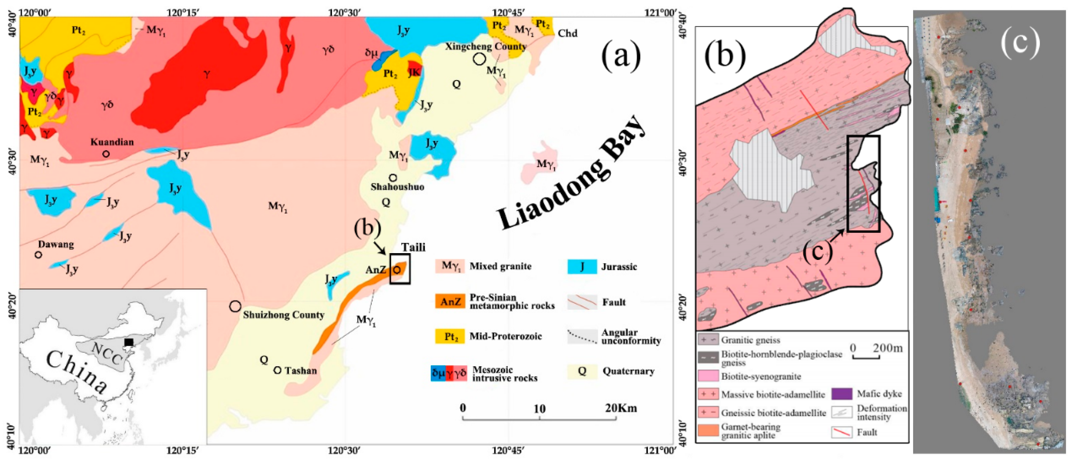
The Archean basement of the eastern North China Craton (NCC) includes the oldest rocks in China (up to ca. 3.8 Ga) [37]. Sediment deposition mainly occurred during the middle to late Proterozoic [38,39,40]. The study area is geographically located in the Xingcheng-Taili region of the western Liaoning Province in northeastern China (Figure 1a), and tectonically in the eastern section of the northern margin of the NCC. It was mapped and investigated in detail regarding its deformation fabrics [41]. A slightly simplified geological map of the study area is shown in Figure 1b.
This area is composed mainly of three granitic suites (Figure 1b), which formed in Neoarchean, Late Triassic, and Late Jurassic times, respectively, and which are also characterized by variable deformation patterns (Figure 1b). These granitic suites are described as follows: (1) The Neoarchean granitic rocks are traditionally referred to as “Suizhong granite”, representing components of the Archean trondhjemite-tonalite-granodiorite (TTG), with a formation age of ca. 2.5 Ga of the NCC’s basement; (2) the Triassic (ca. 220 Ma) granitic rocks, including the porphyritic orthogneiss, garnet-bearing granitic aplite, and biotite-syenogranite, intruded into the Neoarchean gneisses (Figure 1b) [37]; and (3) biotite adamellites with zircon U-Pb age of ca. 150 Ma show a massive structure in the south and a gneissic structure in the north, respectively (Figure 1b). The ductile shear zone of the Taili area is dominantly comprised of granitic rocks deformed within low- to middle-grade metamorphic conditions, which were documented by Liang et al. [39,40,41].
However, in the Taili area, there are still many geological problems to be solved. However, the work of predecessors has mainly focused on the petrology, geochemistry, and chronology of the rock mass [42]. The main rock outcrops in the Taili area are in the intertidal zone (Figure 1c). We can only observe the rock outcrops in about 3 h at the time of the ebb, and it is almost impossible to draw high-resolution geological maps of this area using traditional geological survey methods, which has made research in this area more fragmented. Therefore, making high-quality high-resolution geological maps is of profound significance for unifying geological understanding about the evolution of the NCC [41]. This study aimed to use drones and artificial intelligence algorithms to provide a rapid method of drawing geological sketches. With the help of available geological data in this area, the accuracy of the method can also be convenient verified [37,38,39,40,41,42].
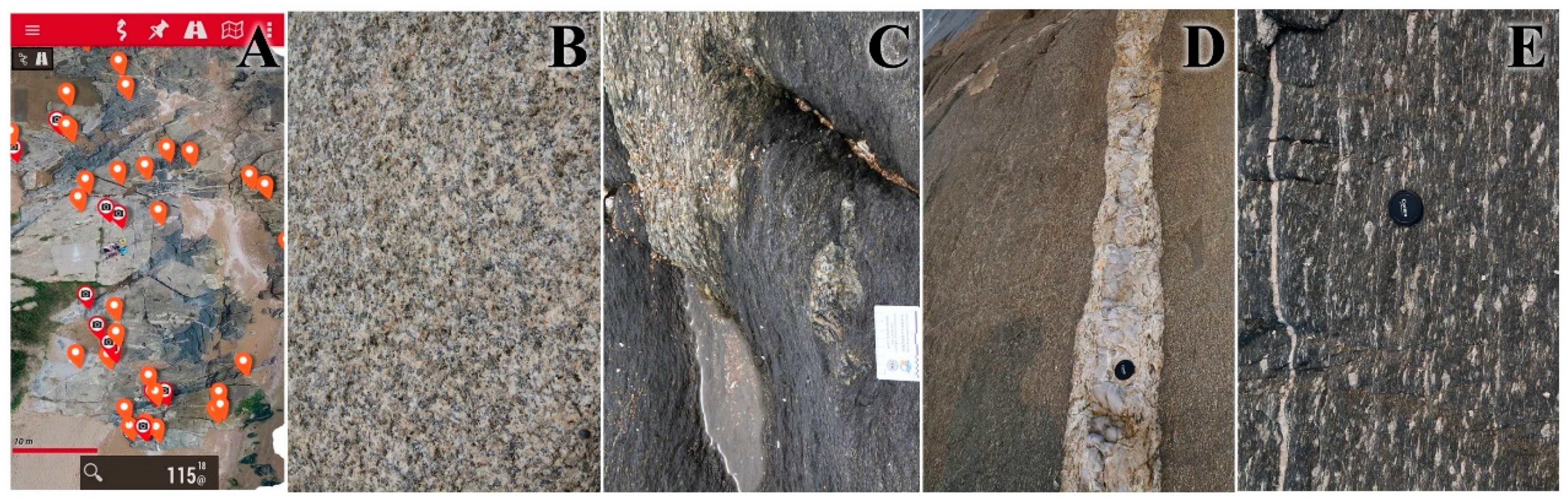
Since 2004, geologists from the College of Earth Sciences of Jilin University have conducted field surveys and measurements of high-resolution lithology-structures in the Precambrian metamorphic crystalline basement rock series exposed in the Xingcheng area, western Liaoning. It was found that the relationship between various lithologies in the metamorphic rock series in this area is complex, undergoing excessive tectonic deformation, as well as multiple alterations of varying degrees of metamorphism and magma. Through field and indoor petrology, zircon U-Pb dating, and other research work, the formation sequence of the main rocks in this area was obtained: ① Quartz dioritic gneiss 2510 Ma ± 7 Ma (Figure 2C); ② mylonite 216.44 Ma ± 0.5 Ma (Figure 2E); ③ pegmatite veins (Figure 2D); and ④ biotite-bearing granite (Figure 2B). The identification of exposed rocks in this area is relatively convenient, and the contact edges of the rock masses are clear, which provides good materials for the lithological image recognition research.
3. Data
3.1. Data Choice
This study used ordinary Red Green Blue (RGB) image data collected by an unmanned aerial vehicle (UAV) as the basic data for classification. There are two reasons: First, ordinary RGB images are easier to obtain, and the cost is lower, which is more important for promoting the popularization of UAVs in geological mapping. Secondly, the UAV can take ultra-resolution RGB images. Although the spectral resolution is poor, its rich texture information can be used as an important parameter. The millimeter-scale spatial resolution can provide geological workers with an observation experience with the naked eye at about a 0.5 m distance. Later work also proved that the use of ultra-resolution color images, combined with the ground truth data in the field, achieved satisfactory recognition accuracy in many scenarios.
We used a DJI Phantom 4 Pro UAV with 1-inch CMOS to take an S-shaped route about 30 m from the ground. The repetition rate of the route was 80%, and the repetition rate of the pictures was 90%. The ground control points were measured using the Real Time Kinematic (RTK)-based Trimble R2 Integrated GNSS Systems. After the images were mosaiced and corrected, the high-resolution orthoimage of the area were obtained by Pix4D. The spatial resolution of image was about 1.3 cm.
3.2. Preprocessing of Data
Machine learning has a very obvious advantage over the traditional algorithm in the field of pattern recognition [43,44,45], but machine learning algorithms generally require the training data shape to be neat [46]. To introduce the machine learning algorithm into high-resolution mapping, we used a slicing method to provide standard-sized source data for machine learning algorithms. The work to determine the slice size needs to be considered in conjunction with the accuracy of geological interpretation. For example, a geological mapping requirement of 1:5000 requires the reflection of a rock vein with a width of 0.5 m on the surface, and it is necessary to identify veins with a width of 0.5 m or less. In this study, a 32 × 32 pixel slice was used with a sampling resolution of approximately 0.35 m.
Geo-interpretation work not only needs to know what the object of interpretation is but also needs to know where the object is, and there is no point in interpreting the object without geographic information [34]. Therefore, in addition to the geological interpretation work, we also needed to geocode the object of interpretation. Geocoding requires a unique ID to match the geographic location, which was not considered in previous image recognition algorithms. In order to facilitate the realization of other functions in the future, we separated geocoding as a functional module, established a WebService-based ground-to-interpret translation server, and used MySQL to store the ID and corresponding geographic location of each point.
In order to get closer to actual work conditions, this study did not remove non-geological-related content, such as tourists, yachts, vegetation, buildings, etc., but classified them separately. We hoped to increase the ability of the model to recognize “foreign objects” during the training of the classification model and improve the generalization and classification accuracy in future applications. Based on the ground conditions in the study area, this study determined the number of interpretations as 7.
The verification area was approximately 50 × 50 m, and the high-resolution image has a spatial resolution of approximately 1.3 cm. A total of 13,432 slices were cut out, each with a pixel size of 32 × 32 pixels and a floor projection area of approximately 0.18 square meters. We divided the high-resolution images of the slices into two groups, namely the training group and the verification group. The amount of each category in each group is shown in Table 1. After grouping, the images and classification tags were formatted as uint8 multidimensional arrays and serialized using the pickle module to facilitate neural network training reading.
In this study, the number of training samples was set to 600 according to the distribution of features in the study area. Except for “Sundries”, “boardwalk”, and “Granite Dykes”, the number of training samples of all other features was less than the number of verification samples. It is worth noting that the training and verification samples were randomly taken from the “verification area”, and their area was only 1/8 of the area of the study area. This means that the number of training samples, the number of validation samples, and the number of objects used for classification was about 1:3:32.
4. Method
4.1. Original Intention of SLIC-CNN
In recent years, deep learning, also known as the deep neural network, has attracted the attention of scholars from all fields [44,45]. A large number of methods about deep learning have been proposed. A typical deep neural network architecture includes a deep belief network (DBN) [46], CNN and auto encoder [25], and so on. Among them, after the first design and optimization of LeCun et al. [47] in 1998, the performance of the deep CNN has increased. In 2015, the CNN classification accuracy surpassed humans on the 1000 class of the ImageNet dataset [47], which contains 1,200,000 training images, 50,000 verification images, and 10,000 test images. The CNN is often designed for the processing of complex signals, such as computer vision; it has shown its superiority compared to other technologies [48]. CNN is widely used in image classification, speech recognition, traffic sign recognition, medical image analysis, and other applications [49]. This effective technique is also applied to the classification of high-resolution and medium-resolution remote sensing images [43,44,45,46]. With more and more research investigating CNN, the number of improved CNNs has increased conspicuously. They are playing an increasingly important role in various fields [50,51,52]. Deep learning is also very suitable for automatic identification of land types in the field since feature selection is not required.
As another important part of deep learning, the accuracy of semantic segmentation technology cannot be compared with pattern recognition. Machine learning, like fully convolutional networks (FCNs), can detect an object’s edges while recognizing it. However, due to the limitation of the algorithm design, FCN directly deconvolves the calculation results of the feature map, so the details of the edge division of complex-shaped objects are not satisfactory.
From recent research, separating the target recognition process from the segmentation process is a more common method to improve the accuracy of recognition and edge segmentation [30,33,34,35,36]. This will not only improve the computing efficiency but also facilitate researchers to optimize recognition and segmentation, respectively.
Superpixel is an effective segmentation solution. It divides the image into a series of sub-regions. Each sub-region has a certain feature between them and has strong consistency. Superpixel segmentation algorithms are also mostly based on color space partitioning and do not care about the meaning of the actual classification. The SLIC superpixel segmentation algorithm [53,54] is a typical representation of this type of algorithm. SLIC seeks the distance of pixels in the image subregion in the International Commission on Illumination Lab color space (CIELAB) color space to determine which pixels need to be clustered into one superpixel region. The algorithm’s processing speed and storage efficiency are superior to other superpixel segmentation algorithms, and the obtained boundary has a strong dependence on the original boundary of the image.
SLIC or other segmentation techniques have become important methods for edge division [55,56]. However, algorithms, such as the iterative self-organizing data analysis technique algorithm (ISODATA), k-mean, and superpixel, all use color information as clustering parameters. What is inside the clustering area does not affect the clustering results. However, the advantage of deep learning algorithms is in determining what an object is. Detecting the spatial location of objects is especially important for automatic geological mapping. So, is there a method to meet the needs of image recognition and spatial positioning? This is the original intention of the SLIC-CNN algorithm.
4.2. Structure of SLIC-CNN
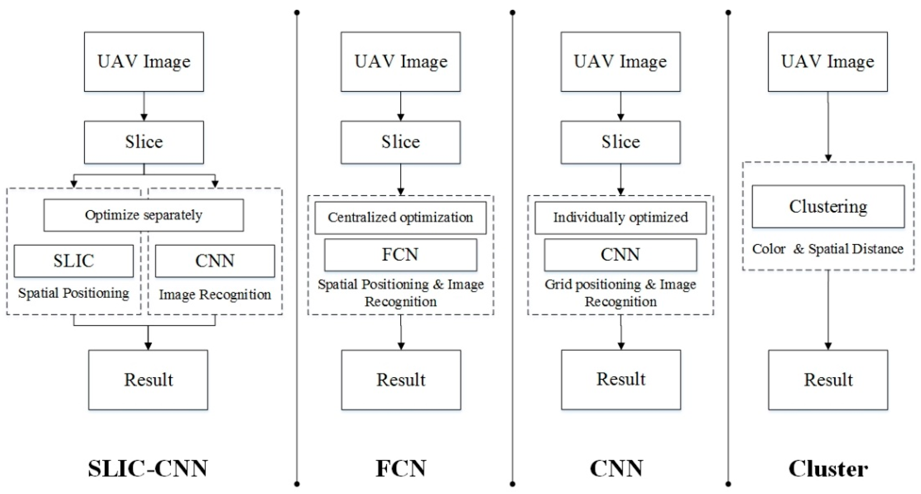
This is shown in Figure 3. Compared with CNN and traditional clustering classification methods, SLIC-CNN separates edge detection from object recognition and optimizes them separately, which can theoretically optimize the image processing results. The parallel design of edge detection and object recognition processes also theoretically improves the efficiency of the algorithm.
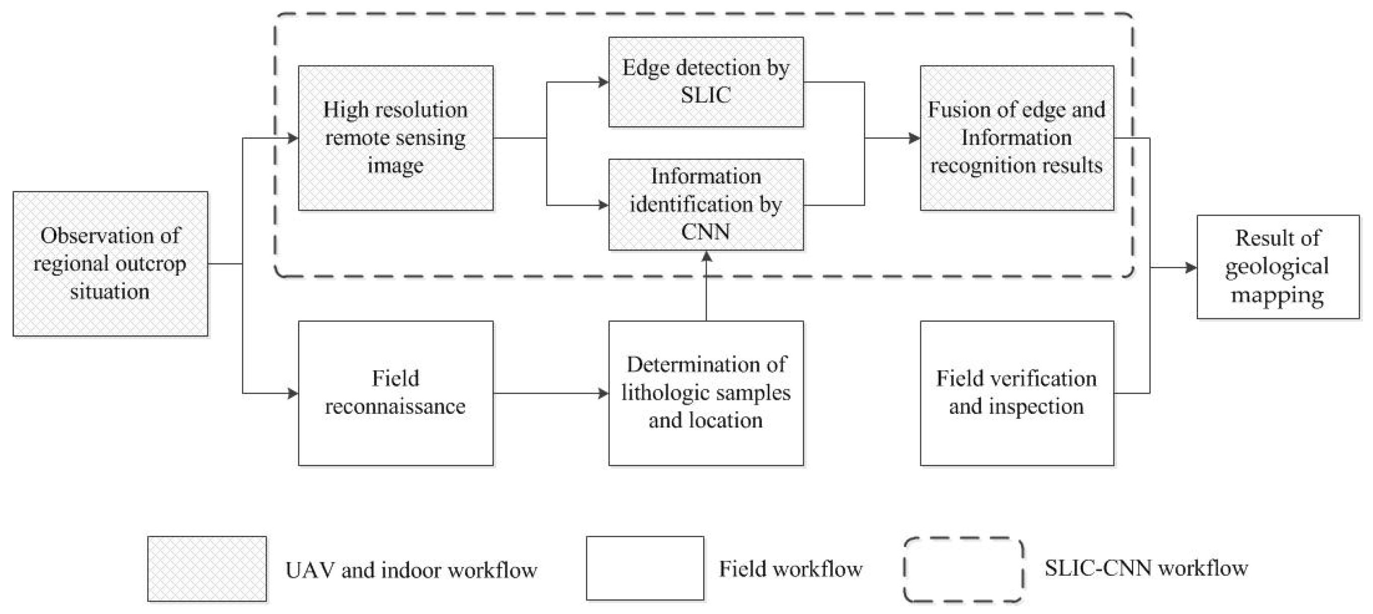
Figure 4 shows the use of UAV-related technology by our team in traditional geological mapping work. As shown in the figure, before geological mapping, in the phase of data acquisition, based on the existing topographic maps and satellite images, we can use the UAV to quickly obtain the geological outcrop photo and topography of the target area. The main purpose of field reconnaissance is to determine the typical lithology and location within the area and provide content control for automatic mapping algorithms. The automatic mapping algorithm based on SLIC-CNN is shown in the dashed box in the figure, and the resulting automatic mapping results still need to use field work inspection and verification. In order to facilitate the comparison of remote sensing images and actual conditions, we used a Smart phone and OruxMaps APP to record the typical lithology of the ground as lithology samples. A total of 74 ground truth samples were collected in the study area for the calibration of the lithology (Figure 2A).
Figure 5 describes in detail the SLIC-CNN method in the high-resolution geological mapping process. In Figure 5, four polygon boxes are drawn in four colors, which represent the four main parts of the SLIC-CNN method. The blue area indicates the generation of high-resolution aerial photography images of UAVs, and the orange area represents the process of convolutional neural network training and classification using high-resolution image slices. The green area represents the process of the SLIC superpixel classification algorithm doing edge division within the study area. The purple area represents the process of using the mode and special decisions to fuse the CNN’s identification content with the edge of the SLIC’s identification.
In detail, after obtaining a high-resolution image, slicing of the image is necessary. This experiment uses ArcGIS fishnet vector data for batch mask slicing, so that the spatial position of each slice can correspond to the vector mask one by one, which is also convenient for geo-coding of the image recognition results. The CNN model was built using the TensorFlow-python framework, which is improved from AlexNet. The SLIC algorithm was also written in python, and the relevant code has been uploaded to github. Finally, ArcGIS’s Python library was used to connect the SLIC and CNN classification results in geographic space, and the slices were assigned values according to the mode principle.
4.3. Deep Learning of SLIC-CNN
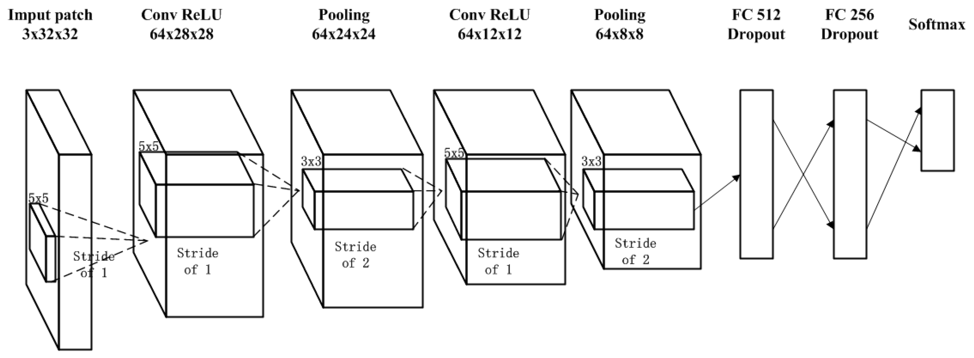
We modeled a machine learning network modeled on the AlexNet. The main parameters are as Figure 6.
The network includes six weighted layers: The first four layers are convolutional layers, so sometimes it is also called convolutional neural networks (CNNs), and the remaining three layers are fully connected layers. The output of the last full-connection layer is sent to a 7-way SoftMax layer, which produces a distribution that covers 7 types of labels. Softmax is a function used to convert the score result into a probability, which is convenient for probability calculation and gradient descent. Our network maximizes the multi-class logistic regression goal, which is equivalent to maximizing the logarithmic probability average of the correct labels in the training sample under the predicted distribution.
The core of the latter convolutional layer is connected to all the core maps in the previous convolutional layer. The neurons in the fully connected layer are connected to all neurons in the previous layer. The response-normalized layer follows the first and second convolutional layers. The pooling layer follows the normalized layer and the fourth convolutional layer.
The first convolutional layer uses 64 kernels with a size of 3 × 5 × 5 and a 1-pixel stride to filter input data with a 3 × 32 × 32 size. The stride is the distance between the centers of the receptive field of the neighboring neuron in the same kernel map. The second convolutional layer needs to take the output of the first convolutional layer (response normalized and pooled) as its own input and filter it with 64 kernels in a 64 × 5 × 5 size. The third convolutional layer has 64 kernels of a 64 × 3 × 3 size connected to the output (convolved, pooled) of the second convolutional layer. The fourth convolution layer has 64 kernels of a 64 × 3 × 3 size. The first full connected layer has 512 neurons and the second has 256, and each full connected layer uses Dropout to guarantee the generalization of the model. We also used random preroll, mirroring, cropping, and stretching to preprocess the data before the data reading process to enhance the generalization ability of the model.
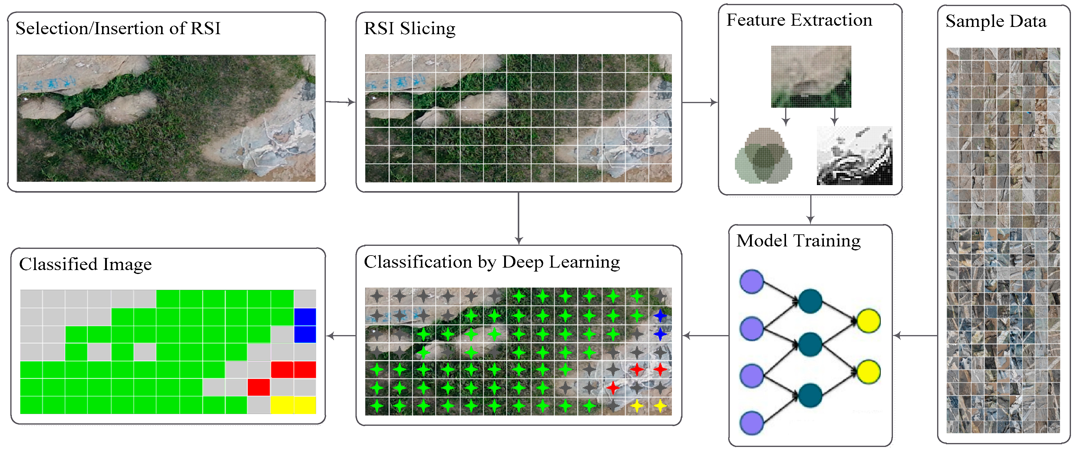
In this study, CNN were mainly used for the recognition of ground objects. The purpose was to accurately segment slices of high-resolution images into seven predefined categories. However, this method of surface classification of slices cannot accurately locate the edge of the feature (Figure 7). To solve this problem, we introduced a superpixel classification method in the process of high-resolution mapping.
4.4. Superpixel of SLIC-CNN
The SLIC algorithm mainly uses the K-means clustering algorithm to process superpixels. The distance measurement in the clustering algorithm not only includes the color distance of the color space but also the Euclidean distance of the pixel coordinates. Therefore, the center point of the K-means cluster consists of five-dimensional vectors. This includes the recording of pixels in the lab color space and the XY coordinates of the pixel. Since XY coordinates cannot be directly calculated with the color space, a compactness parameter is added [57,58].
In addition, after the K-means clustering, a convolution process is also needed in order to merge independent pixels enclosed by a region into a certain class. The cluster center K parameter is used to indicate the number of segmentation results. The optimization of these parameters needs to be considered in combination with the complexity of geological conditions and the accuracy of mapping. After many experiments, our team believes that the number of segments in the SLIC algorithm should be set to a suitable value first, so that the initial cluster center distance of the SLIC algorithm is approximately equal to the step size of the CNN training slice. If the number of segments is too large, and the image segmentation is too fine, it can achieve better results for object segmentation and edge recognition, but it will cause many regions to not correspond to the classification result. If this number is too small, it will result in a small number of segments, although it can reduce the appearance of areas without corresponding classification results, but the edge fitting effect is poor (Figure 8). It can be seen that when the SLIC clustering center step ≈ CNN slice step length, there are few missing maps, the SLIC segmentation area is approximately equal to the CNN segmentation window size, and the edge matching is better. When the SLIC clustering center step >> CNN slice step size, although almost no missing map spot is apparent, the segment number is too small, and the spot edge is too sketchy. When the SLIC clustering center step size << CNN slice length, the segment number is more, and the edge fitting is better. However, there are more spots missing.
When using the SLIC algorithm and appropriate parameters, we can obtain more satisfactory results of edge partitioning. Based on the edge division, we combined the content recognition results of machine learning to theoretically obtain the classification results of the accurate edges and accurate content. However, there are still some content and scope matching problems that need to be solved. Our team has proposed a “mode and special decision” method to solve these topological issues.
4.5. Mode and Special Decision of SLIC-CNN
For the segmented image, how to assign each segment to the label obtained by the deep learning needs careful consideration. Simply use of CNN’s labels to assign SLIC segments is not enough. Especially, in areas with complex geological conditions, we need to be especially cautious. For geological mapping work, many small segments have important geological significance, such as dykes and intrusions. The superpixel segmentation algorithm can adjust the parameters to segment these fine geological bodies as much as possible. However, the depth learning algorithm does not increase the sampling rate indefinitely. Our research shows that the accuracy of prediction is greatly reduced when the pixel resolution of the recognition target is from 64 px, 32 px, to 16 px. Even at a resolution of 64 px, taking this article as an example, the corresponding sampling step on the ground reaches 7 cm. There are still many gaps from the high-resolution mapping specifications promulgated by China (more than 5 cm width veins need to be identified). Therefore, the separation of finely segmented segments from the background and achieving good-quality labels must be considered. In response to this, our team proposed a method called “mode and special decision” to solve this problem.
The meaning of mode and special decision is to use different decision-making schemes to define the target content for different situations. The mode here refers to the most frequently occurring tag in the range of segment slices generated by an SLIC. We superimposed CNN identified classification tag points and SLIC classification segments in space. The following situations thus occured:
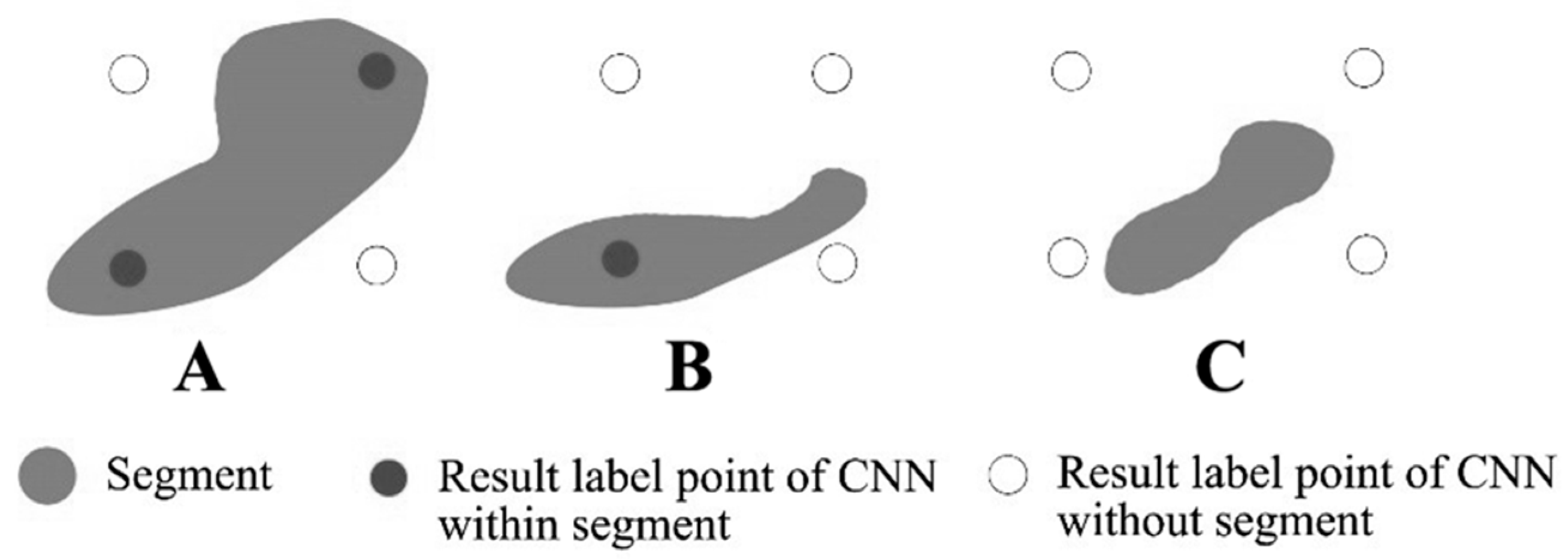
For the Figure 9A case, we named the segment using the most number of tags that appear in the segment. Since it is considered that the mode may not be the majority (50%), we needed to use the Top_K method to output the first three classifications with the highest prediction rate when they wee output at the softmax layer, and add the comparisons to obtain the classification with the highest total probability. The Figure 9B situation is much simpler. We could directly assign the CNN classification result to this segment.
In the case of Figure 9C, we needed to leave the class as null at this region and then use the nibble algorithm to assign it. The nibble algorithm assigns the value of the nearest neighbor to the target area. The algorithm performs internal Euclidean allocation and assigns the nearest neighbor values to each target area.
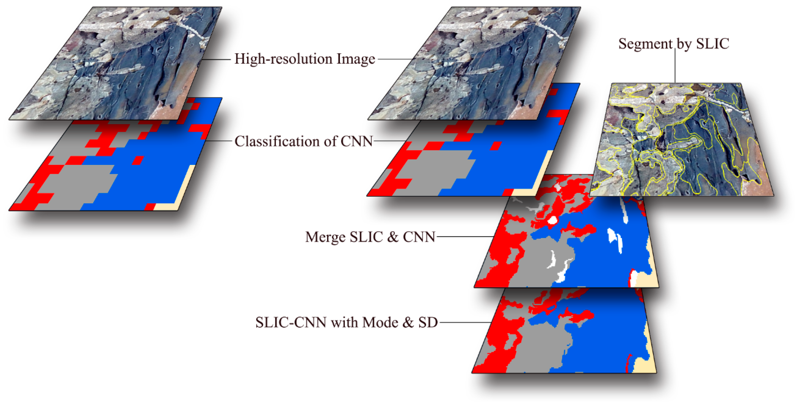
By merging the SLIC and CNN, we established a high-resolution geological mapping method based on SLIC-CNN. This method is based on the use of deep learning classification of high-resolution remote sensing slices. Using SLIC classification methods to determine the classification boundary, the two are combined by the mode and special decision principles, resulting in the final high-resolution mapping results (Figure 10).
In this experiment, we built a SLIC-CNN algorithm platform based on the Python version of the Tensorflow framework. The experimental hardware platform was a dual-channel Intel Xeon E5-2630V4, with the nVIDIA Quadro K5200 model GPU.
5. Result
5.1. Optimization of CNN
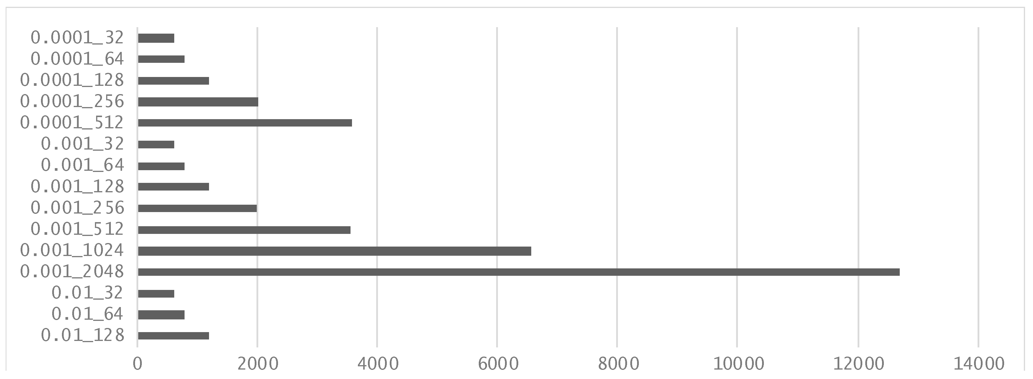
In order to find the best parameters of CNN, we used a total of 15 parameter combinations. In the case of a certain number of iterations, the total calculation time is closely related to the batch size. In the model training–accuracy line chart, we can find that with a certain number of iterations, the higher the batch size setting, the more time consuming the calculation; the smaller the learning rate setting, the slower the model converges. However, at the same time, according to the verification of the correct rate line graph, if the batch size is set too high, it will cause large fluctuations in the accuracy rate of the model validation (batch 1024 and batch 2048 in Figure 11). Setting the learning rate too high (0.01) can also cause the model validation to fluctuate correctly and have poor convergence.
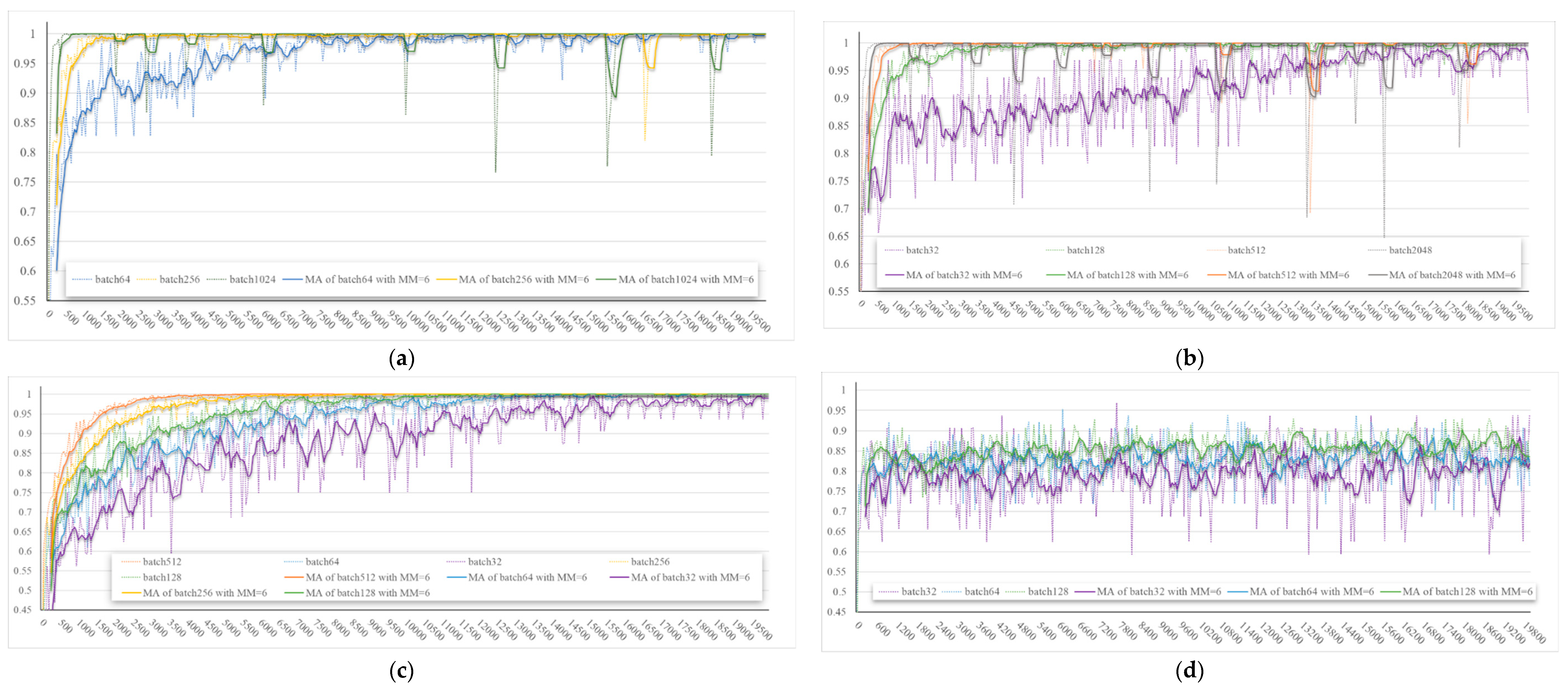
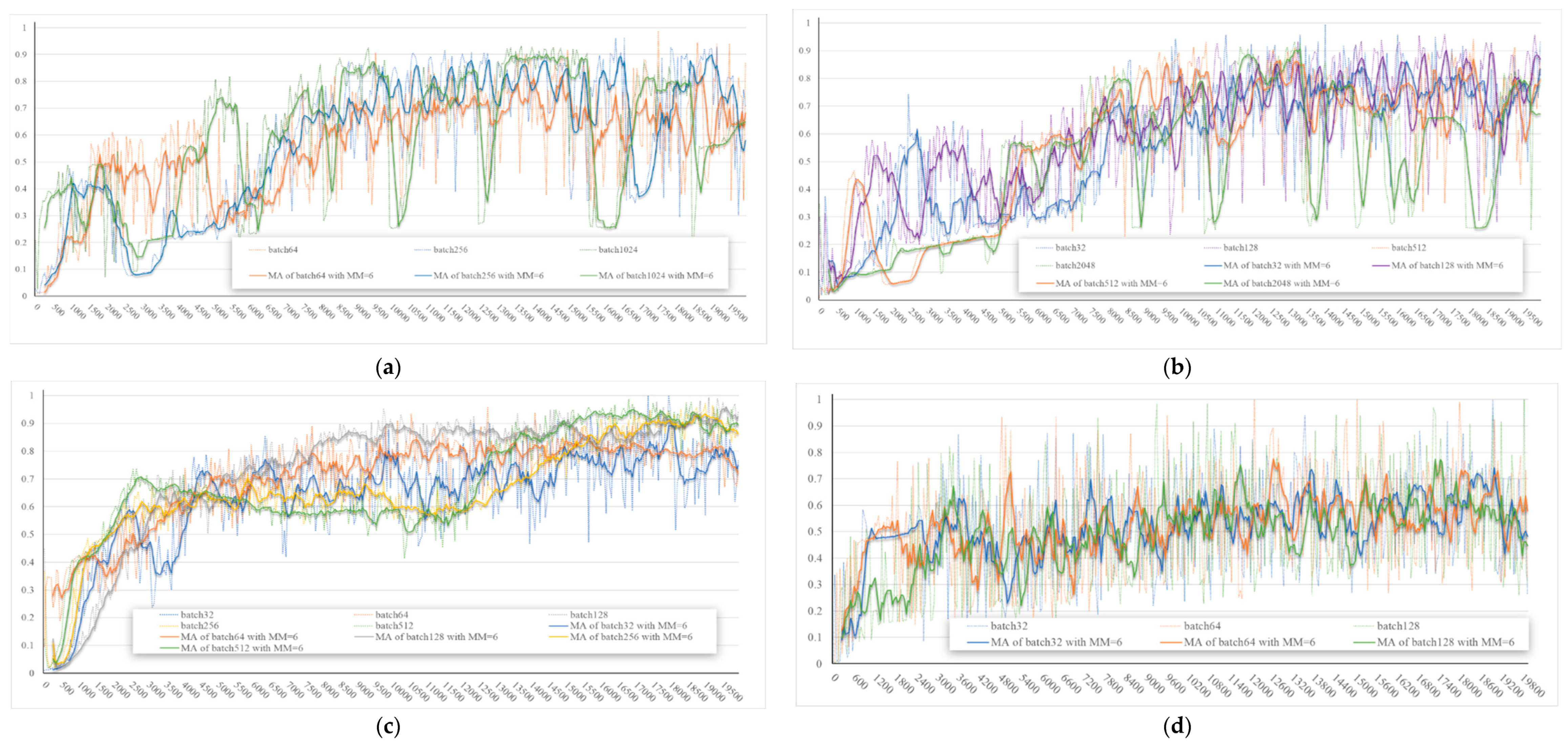
From Figure 11, we can compare the average correct rate of each model, but we cannot see whether this correct rate is stable or not. After considering Figure 12, Figure 13 and Figure 14, and after several experiments and multiple comparisons, we selected the 0.0001 learning rate and 512 batch size training model as application models to participate in the SLIC-CNN mapping work.
5.2. Optimization of SLIC
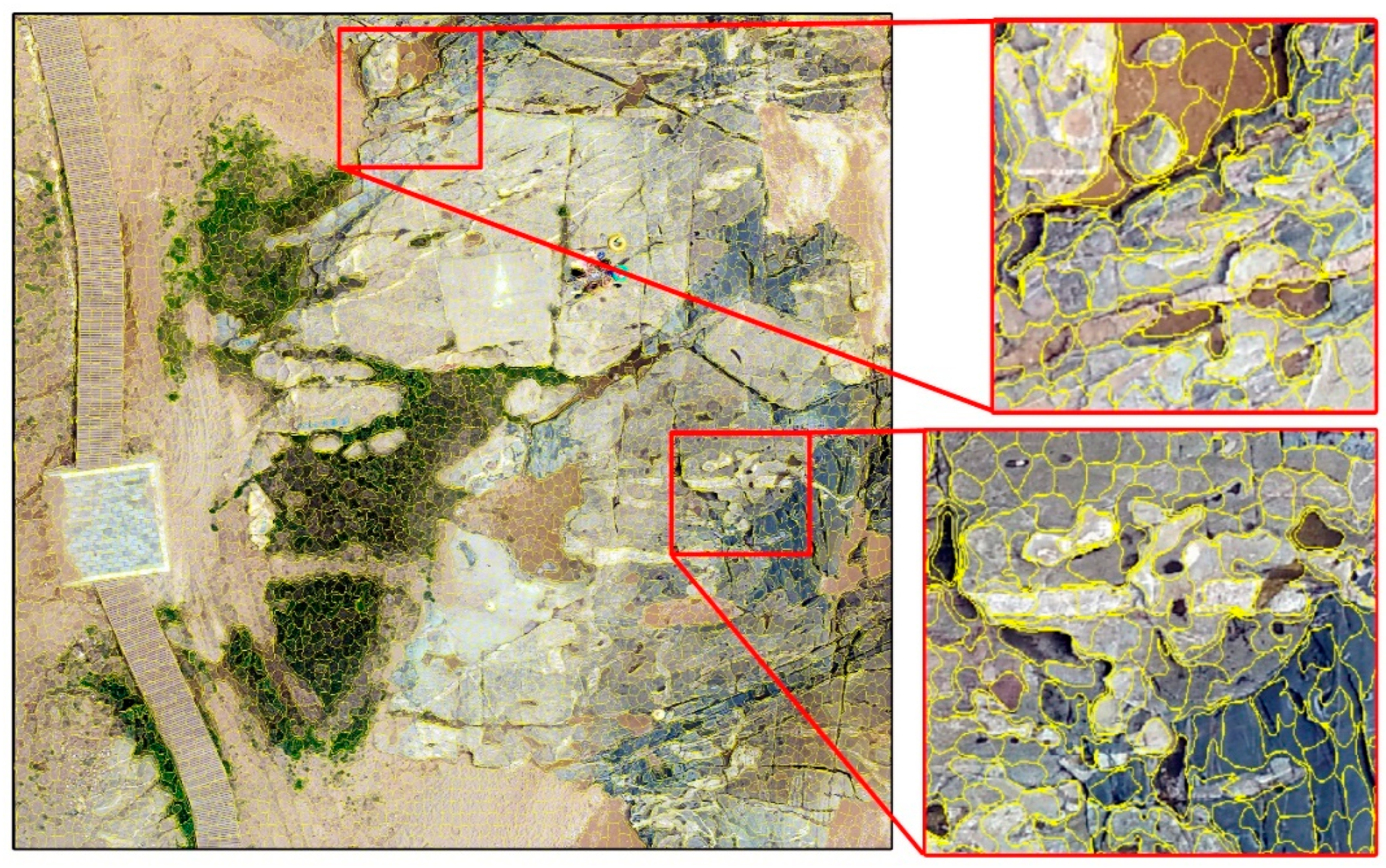
In the parameters of the SLIC algorithm, n_segments or K parameters control the number of slices. The sigma parameter affects the Gaussian smoothing operator, the max_iter parameter controls the number of smooth iterations, and the max_iter and sigma parameters control the K-means clustering effect together. The compactness parameter balances the relationship between the color space and distance. Through the combination of different parameters, we can obtain a variety of segmentation combinations. According to previous calculations, the number of deep learning slices in the study area is 13,432, and the number of SLIC segments should not exceed this value. In order to find the best segmentation parameters, we performed 165 experiments for n_segments from 350–10,000, sigma from 0–8, and compactness from 0.2–50, and selected the segmentation result with the best edge fitting effect. That is, n_segments = 8000, sigma = 6, and compactness = 5 (Figure 15). From the figure, we can see that the SLIC algorithm can better fit the edge of the segment with the edge of the ground object. Although some concentric ring segments are generated, we only need the SLIC to mark the effective edge to complete the task. The merging of segments does not belong to the SLIC algorithm.
After obtaining the segmentation results of the SLIC and the recognition results of the AlexNet, then the process of mode and special decision, we can finally obtain the results of high-resolution geological mapping of the study area.
5.3. Results of SLIC-CNN
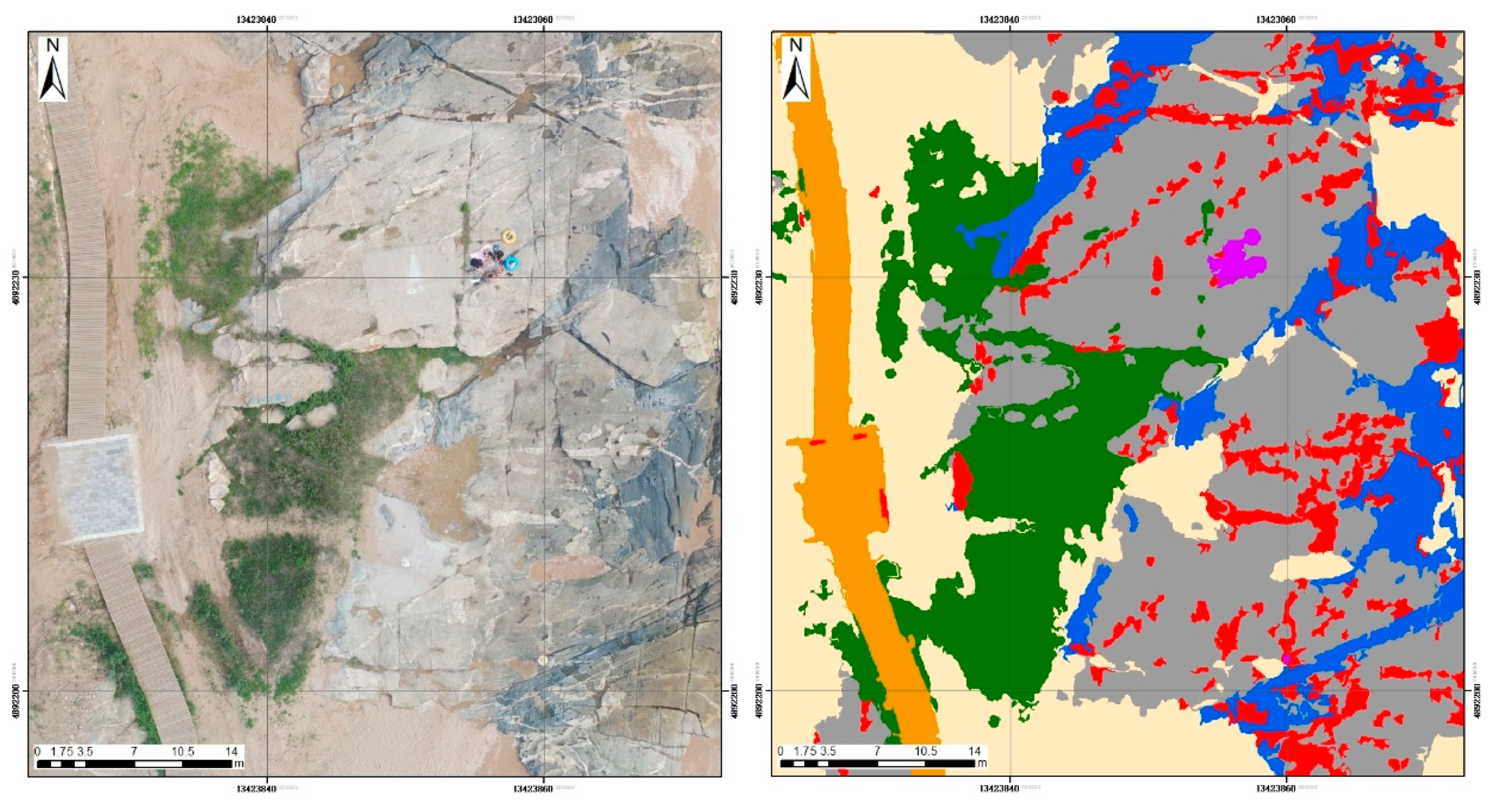
Compared with Figure 16, we can see that the SLIC-CNN algorithm can accurately identify the exposed terrain in the area, and the annotation of the edge of the terrain is also more elaborate. The boundaries between mylonites and orthogneiss, the boundaries between plants and beaches, and the boundaries between roads and beaches are all more accurate.
In order to compare with the classification results of the existing classification methods, we also experimentally classified and interpreted the study area using the pixel classification based on the maximum likelihood method (Table 2) and the object-oriented classification based on the k-Nearest Neighbor (KNN) method (Table 3). In the object-oriented classification, we performed many experiments and comparisons. The classification effect was best when the scale parameter was set to 90, the merge parameter was set to 95, and the texture kernel size was set to 5.
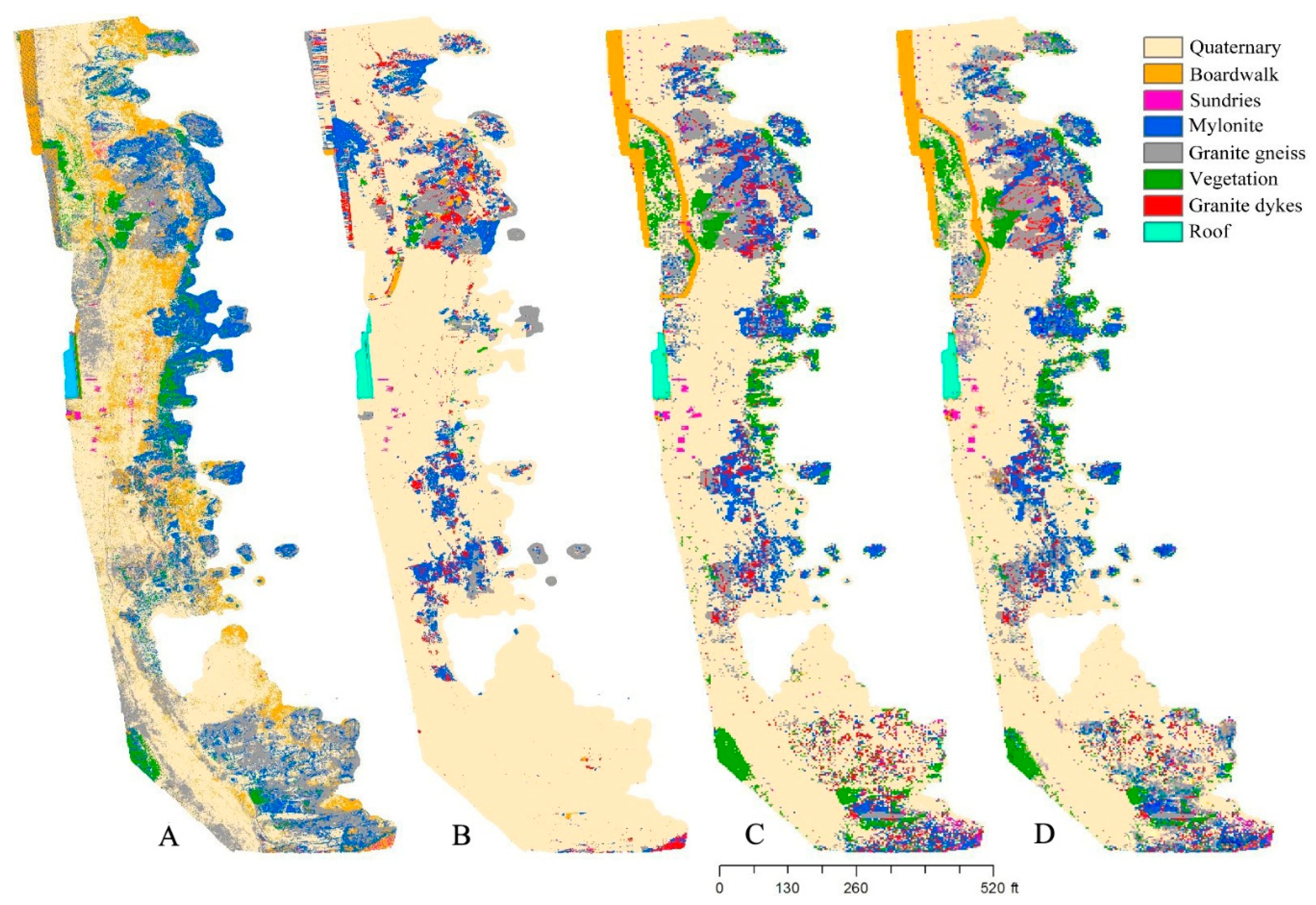
After deriving the classification results and confusion matrix of those classification methods, we visually compared the mapping accuracy of the four methods in the high-resolution mapping work (Figure 17).
The confusion matrix is an intuitive tool for displaying multi-class results. Cells (x, y) represent the proportion of objects in x that are classified into y. According to this, it can be found that the overall recognition hits of the pixel-based method are better than the object-oriented method, especially for Mylonite. The CNN method shows far better hit rates than the pixel-based and object-oriented methods (Table 4). This is consistent with the advantages shown by deep learning algorithms in other image recognition fields. Except for “sundries”, SLIC-CNN has a higher hit rate than the CNN method (Table 5). The Kappa verification result of SLIC-CNN is k = 0.8523, which is also greater than the AlexNet method (k = 0.8426).
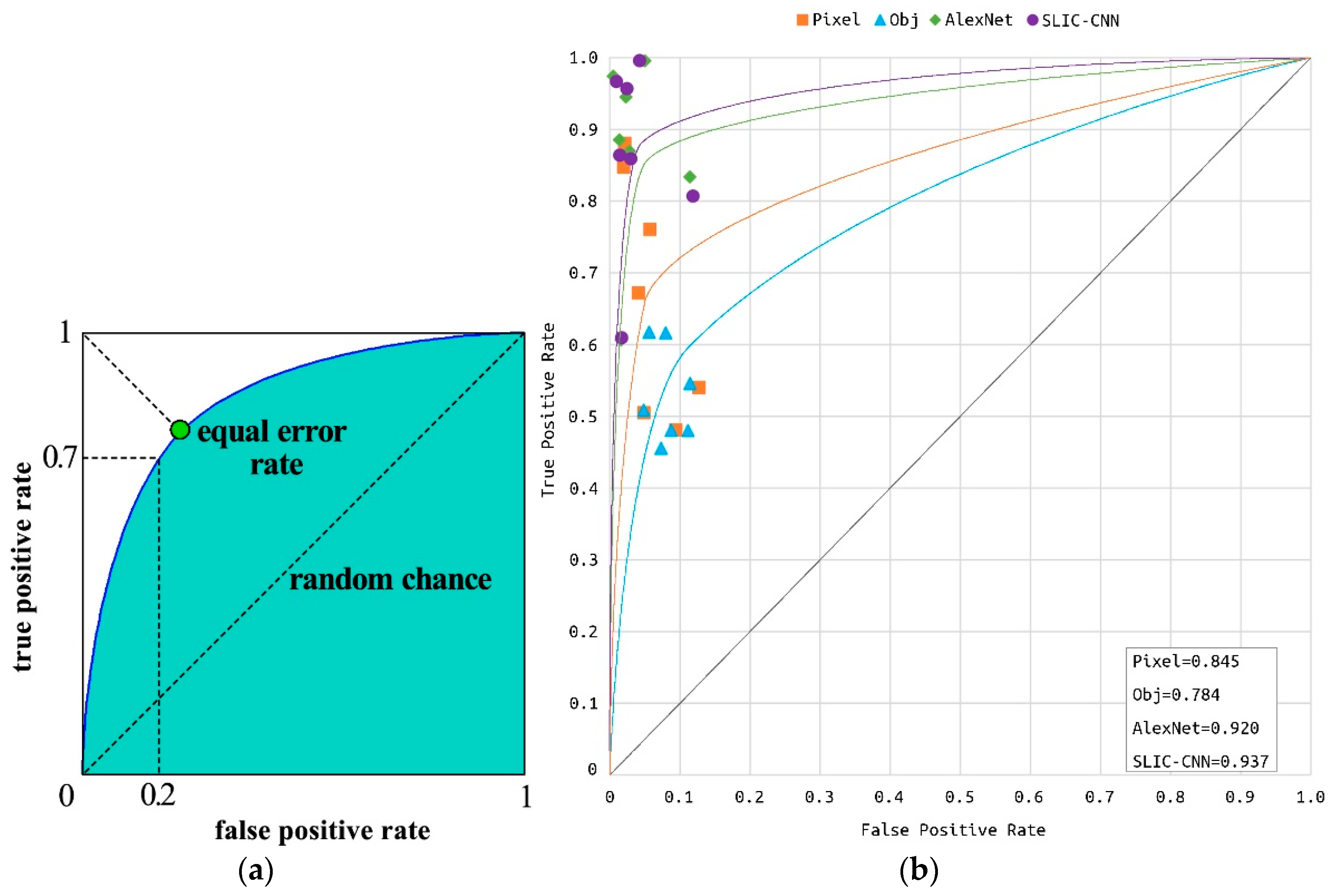
To more intuitively compare the results of the four methods, we used the Receiver Operating Characteristic (ROC) curve (Figure 18a). ROC (receiver operating characteristic curve) is a comprehensive indicator reflecting the continuous variables of sensitivity and specificity. It uses the composition method to reveal the relationship between the sensitivity and specificity. It uses the sensitivity as the ordinate and (1-specificity) as the abscissa to draw a curve. The larger the area under the curve (AUC), the higher the diagnostic accuracy. On the ROC curve, the point closest to the upper left of the graph is a critical value with a higher sensitivity and specificity. In this case, the AUC of the SLIC-CNN algorithm was 0.937, higher than the AlexNet slice classification (0.92), pixel-based method (0.845), and object method (0.784) (Figure 18b).
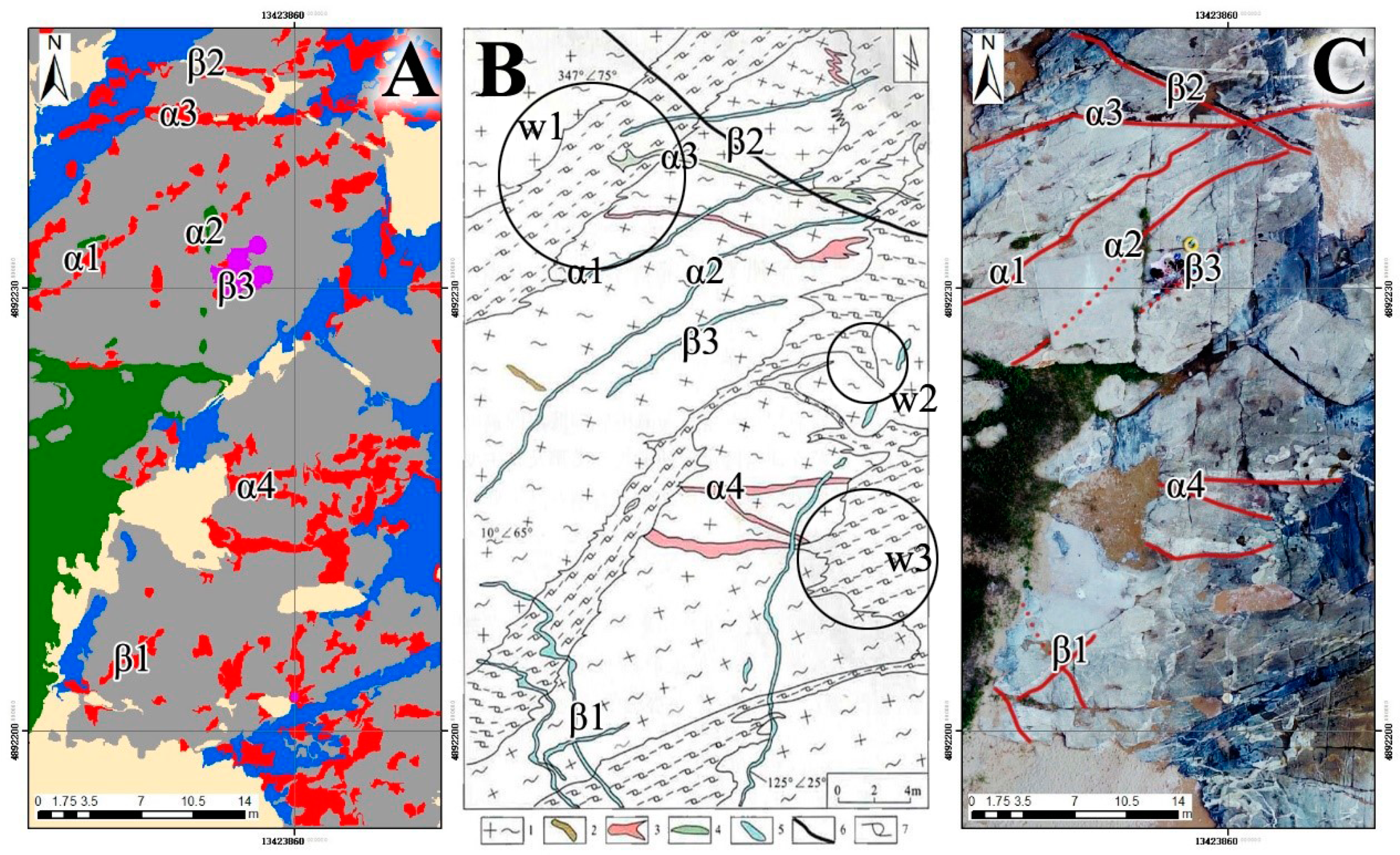
Using SLIC-CNN mapping results in comparison with the available geological data (Figure 19), some features of the UAV high-resolution geological mapping method can be found. For ease of comparison and illustration, we marked the typical dykes with the same Latin symbol in the map and marked them with dark red lines under the typical veins on the remote sensing image. The part covered by concrete or beach due to human factors is indicated by the dark-red dotted line. SLIC-CNN mapping is better at identifying veins at α1 in the figure, but it is still not continuous enough. Compared with remote sensing images, we found that the exposed part of the α1 dyke gradually became thin and the algorithm could not identify it. The southern part of the α2 dike was covered by a newly built cement table, and the ground was blocked by tourists at β3, which made it impossible to identify the veins in the area. In addition, the recognition of veins at α3 was very effective, and the “S”-shaped dykes were also identified at α4. The veil at β1 was too small and resulted in poor recognition. The basic dyke at β2 was identified by the algorithm as sand deposition. In general, SLIC-CNN has a high recognition rate for the edge and content of rock masses, and its identification of veins can also give a partial reference.
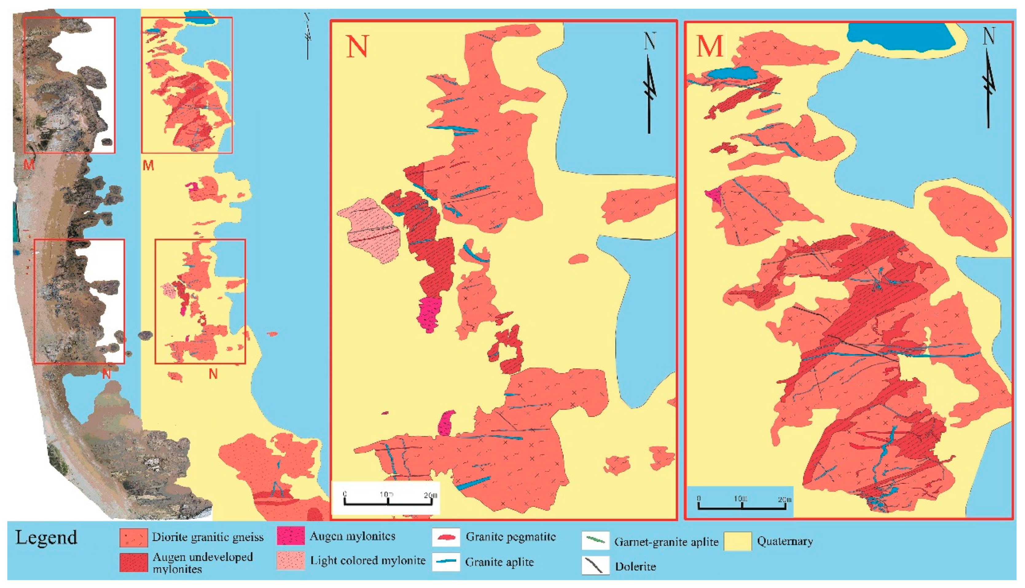
Figure 19b is a fine tectonic lithologic geological map drawn by Jin Wei and Zheng Changqing, College of Earth Sciences, Jilin University in 2004. This map has been the most detailed geological map of the region for a long time. However, it can be found that the edges of the mylonite body are drawn inaccurately in the picture (w1, w2, and w3 in Figure 19b). The result of the automated geological mapping process (Figure 18a) is in the shapefile format, which is a working and interchange format promulgated by Environmental Systems Research Institute, Inc. (ESRI) for simple vector data with attributes, and it is very convenient for merging, cropping, and adjusting attributes. On the basis of Figure 18a, the data obtained from the ground survey perfected the automated results, resulting in a high-resolution geological map of Taili area (Figure 20). Compared with previous studies, this geological map has higher resolution and coverage. Moreover, thanks to the assistance of the automated SLIC-CNN method, it took only half a day to draw this map, which has greatly improved the efficiency compared to the traditional geological survey method.
6. Discussions
The popularity of UAV has brought about an opportunity to solve the geological survey problems in difficult areas. Although we minimized the ground geological operations in this experiment, the high-resolution geological mapping work that appears to be automated is still inseparable from a certain amount of ground geological work. At this stage, it is limited by image conditions and it is not yet possible to accurately distinguish certain lithologies, such as pegmatites and fine-grained rocks, in this study area. However, it can be seen from Table 5 that, even with the SLIC-CNN method, the correct classification rate of dykes in the study area remains low. This is related to the actual data used in the experiment. The spatial resolution of the real data used in this experiment reached 3 cm, and almost all of the small dykes in the study area were plotted. In addition, it is worth noting that UAVs and cameras cannot collect rock information covered by sand, soil, or vegetation. This limits the application of automated geological surveys. There are still many studies to be done on the application of automation in the field of geological mapping.
However, with experiments, it was found that the use of UAVs and deep learning algorithms in traditional geological mapping work provides a huge increase in work efficiency, and its mapping accuracy is also satisfactory. UAV technology brings new solutions to ground geological surveys.
Automatic detection lithology boundaries have been proven to greatly improve the efficiency of geological mapping [59]. This experiment used CNN on the basis of Vasuki’s experiment to further improve the automation of mapping. Compared with traditional classification, the use of SLIC-CNN could detect lithology and boundaries more accurately and automatically. Additionally, the SLIC-CNN technology provides important ideas for automated geological mapping. With high-accuracy image recognition technology, we believe that future geological surveys will become more automatic and intelligent: UAVs will fly according to routes and take ground images, and important geological phenomena in the images will be quickly identified and positioning. Related information will be sent back to the server and quickly mapped. Significant areas and uncertain areas will be identified for geologists to conduct ground investigations.
7. Conclusions
In this study area, the results of a new large-scale mapping process can be said to be satisfactory. The effect of accelerating the use of UAVs and deep learning algorithms is obvious. The results of the SLIC-CNN method were much better than traditional image classification methods, like CNN and AlexNet, for geological body discrimination and the fitting effect of the rock mass edge, which was further improved compared with the ordinary deep learning method. Compared with traditional geological surveys, more accurate rock mass mapping results can be obtained with the help of drone images. Although the automatic classification results of SLIC-CNN were inadequate for rock vein recognition, the accuracy of other rock mass mapping was impressively satisfied. Additionally, it can greatly reduce the manual labor of high-resolution mapping and produce a high-resolution geological sketch with high classification accuracy in less time. Based on the UAV, SLIC-CNN method, and further tectonic evidence, we obtained results of the high-resolution geological map and the ductile shear deformation zone in the region, and confirmed the results of previous studies on the ductile shear zone in the Taili area. The SLIC-CNN method accelerates the interpretation of high-resolution remote sensing images, improves the accuracy, and makes the classification results more convincing for geology.
Therefore, the application effect of the SLIC-CNN algorithm in the field of geological mapping is satisfactory and worth promoting. These methods and results will provide very useful experience for subsequent geological work, and will greatly enrich the means of geological research by relieving personnel and environmental pressures in field surveys.
Author Contributions
Resources, Linfu Xue; Funding acquisition, Xiaoshun Li; Software, Xiangjin Ran; Writing—original draft, Xuejia Sang; Writing—review & editing, Jiwen Liu and Zeyu Liu. All authors have read and agreed to the published version of the manuscript.
Funding
The Project Supported by the National Natural Science Foundation of China (71704177, 71874192), the Open Fund of Key Laboratory of Coastal Zone Exploitation and Protection, Ministry of Natural Resource (No.: 2019CZEPK11) and the Fundamental Research Funds for the Central Universities (2019CXNL08, 2019ZDPY-RH02).
Acknowledgments
Thanks to Jianxiong Ma, Yangzhao Zheng, Chuanqi Dai and other members of Digital Geoscience Research Center, College of Earth Sciences, Jilin University.
Conflicts of Interest
The authors declare no conflict of interest.
References
- Latifovic, R.; Pouliot, D.; Campbell, J. Assessment of Convolution Neural Networks for Surficial Geology Mapping in the South Rae Geological Region, Northwest Territories, Canada. Remote Sens. 2018, 10, 307. [Google Scholar] [CrossRef] [Green Version]
- Sean, P.B.; Steven, M.; Darren, T.; Mike, R.J.; Sinan, A.; Sam, T.T.; Hasnain, A.B. Ground-based and UAV-Based photogrammetry: A multi-scale, high-resolution mapping tool for structural geology and paleoseismology. J. Struct. Geol. 2014, 69, 163–178. [Google Scholar]
- Balestro, G.; Piana, F. The representation of knowledge and uncertainty in databases of GIS geological maps. Ital. J. Geosci. 2007, 126, 487–495. [Google Scholar]
- Nataliia, K.; Mykola, L.; Sergii, S.; Andrii, S. Deep Learning Classification of Land Cover and Crop Types Using Remote Sensing Data. IEEE Geosci. Remote Sens. Lett. 2017, 14, 778–782. [Google Scholar]
- Almalki, K.A.; Bantan, R.A.; Hashem, H.I.; Loni, O.A.; Ali, M.A. Improving geological mapping of the Farasan Islands using remote sensing and ground-truth data. J. Maps 2017, 13, 900–908. [Google Scholar] [CrossRef]
- Jones, R.R.; Mccaffrey, K.J.W.; Wilson, R.W.; Holdsworth, R.E. Digital field data acquisition: towards increased quantification of uncertainty during geological mapping. Geol. Soc. Lond. Spéc. Publ. 2004, 239, 43–56. [Google Scholar] [CrossRef] [Green Version]
- Chatterjee, S.; Bhattacherjee, A.; Samanta, B.; Pal, K.S. Image-based quality monitoring system of limestone ore grades. Comput. Ind. 2010, 61, 391–408. [Google Scholar] [CrossRef]
- Li, J.; Jin, W.; Zheng, P.; Zhang, X. Geochemical Characteristics and Zircon U-Pb Geochronology of the Biotite Adamellite in Taili Area, Western Liaoning Province. J. Jilin Univ. Earth Sci. Ed. 2014, 44, 1219–1230. [Google Scholar]
- Kroupi, E.; Kesa, M.; Navarro, V.; Saeed, S.; Pelloquin, C.; Alhaddad, B.; Moreno, L.; Soria, A.; Ruffini, G. Deep convolutional neural networks for land-cover classification with Sentinel-2 images. J. Appl. Remote Sens. 2019, 13, 024525. [Google Scholar] [CrossRef]
- Tao, Y.; Xu, M.; Zhong, Y.; Cheng, Y. GAN-Assisted Two-Stream Neural Network for High-Resolution Remote Sensing Image Classification. Remote Sens. 2017, 9, 1328. [Google Scholar] [CrossRef] [Green Version]
- Fu, G.; Liu, C.; Zhou, R.; Sun, T.; Zhang, Q. Classification for High Resolution Remote Sensing Imagery Using a Fully Convolutional Network. Remote Sens. 2017, 9, 498. [Google Scholar] [CrossRef] [Green Version]
- Ferreira, A.; Giraldi, G. Convolutional Neural Network approaches to granite tiles classification. Expert Syst. Appl. 2017, 84, 1–11. [Google Scholar] [CrossRef]
- Cracknell, M.J.; Reading, A.M. The upside of uncertainty: Identification of lithology contact zones from airborne geophysics and satellite data using random forests and support vector machines. Geophysics 2013, 78, 113–126. [Google Scholar] [CrossRef]
- Hesamian, M.H.; Jia, W.; He, X.; Kennedy, P. Deep Learning Techniques for Medical Image Segmentation: Achievements and Challenges. J. Digit. Imaging 2019, 32, 582–596. [Google Scholar] [CrossRef] [PubMed] [Green Version]
- Jia, F.; Lei, Y.; Guo, L.; Lin, J.; Xing, S. A neural network constructed by deep learning technique and its application to intelligent fault diagnosis of machines. Neurocomputing 2018, 272, 619–628. [Google Scholar] [CrossRef]
- Tang, J.; Deng, C.; Huang, G.B.; Zhao, B. Compressed-Domain Ship Detection on Spaceborne Optical Image Using Deep Neural Network and Extreme Learning Machine. IEEE Trans. Geosci. Remote Sens. 2015, 53, 1174–1185. [Google Scholar] [CrossRef]
- Xianju, L.; Xinwen, C.; Weitao, C.; Gang, C.; Shengwei, L. Identification of Forested Landslides Using LiDar Data, Object-based Image Analysis, and Machine Learning Algorithms. Remote Sens. 2015, 7, 9705–9726. [Google Scholar]
- Sharma, A.; Liu, X.; Yang, X.; Shi, D. A patch-based convolutional neural network for remote sensing image classification. Neural Netw. 2017, 95, 19–28. [Google Scholar] [CrossRef]
- Wang, Q.L.; Jin, W.; Cai, L.B.; Cui, X.H.; Zhang, Q.; Wu, C.S. Characteristics and genesis of Neoarchean granitic complex in Xingcheng of western Liaoning. Glob. Geol. 2012, 31, 479–492, (In Chinese with English abstract). [Google Scholar]
- Patel, A.K.; Chatterjee, S. Computer vision-based limestone rock-type classification using probabilistic neural network. Geosci. Front. 2016, 7, 53–60. [Google Scholar] [CrossRef] [Green Version]
- Krizhevsky, A.; Sutskever, I.; Hinton, G. ImageNet classification with deep convolutional neural networks. Neural Inf. Process. Syst. 2012, 25, 1145–1155. [Google Scholar] [CrossRef]
- Bejiga, M.B. A Convolutional Neural Network Approach for Assisting Avalanche Search and Rescue Operations with UAV Imagery. Remote Sens. 2017, 9, 100. [Google Scholar] [CrossRef] [Green Version]
- Dimitrios, M.; Mihai, D.; Thomas, E.; Uwe, S. Deep Learning Earth Observation Classification Using ImageNet Pretrained Networks. IEEE Geosci. Remote Sens. Lett. 2016, 60, 105–109. [Google Scholar]
- Guidici, D.; Clark, M.L. One-Dimensional Convolutional Neural Network Land-Cover Classification of Multi-Seasonal Hyperspectral Imagery in the San Francisco Bay Area, California. Remote Sens. 2017, 9, 629. [Google Scholar] [CrossRef] [Green Version]
- Bouvrie, J. Notes on Convolutional Neural Networks. Neural Nets 2006, 47–60, in practice. [Google Scholar]
- Ji, S.; Zhang, C.; Xu, A.; Shi, Y.; Duan, Y. 3D Convolutional Neural Networks for Crop Classification with Multi-Temporal Remote Sensing Images. Remote Sens. 2018, 10, 75. [Google Scholar] [CrossRef] [Green Version]
- LeCun, Y.; Bengio, Y.; Hinton, G. Deep learning. Nature 2015, 521, 436. [Google Scholar] [CrossRef]
- Abadi, M. TensorFlow: Learning functions at scale. Acm Sigplan Not. 2016, 51, 1. [Google Scholar] [CrossRef]
- Zheng, C.G.; Yuan, D.X.; Yang, Q.Y.; Zhang, X.C.; Li, S.C. UAVRS Technique Applied to Emergency Response Management of Geological Hazard at Mountainous Area. Appl. Mech. Mater. 2013, 239–240, 516–520. [Google Scholar] [CrossRef]
- Machado, G.M.; Jabor, P.; Coelho, A.; Albino, J. Geohistorical evolution and the new geological map of the city of Vitoria, ES, Brazil. Ocean Coast. Manag. 2017, 10, 151. [Google Scholar] [CrossRef]
- Tziavou, O.; Pytharouli, S.; Souter, J. Unmanned Aerial Vehicle (UAV) based mapping in engineering geological surveys: Considerations for optimum results. Eng. Geol. 2017, 11, 232–250. [Google Scholar] [CrossRef] [Green Version]
- Yathunanthan, V.; Eun-Jung, H.; Peter, K.; Steven, M. Semi-automatic mapping of geological Structures using UAV-based photogrammetric data: An image analysis approach. Comput. Geosci. 2014, 69, 22–32. [Google Scholar]
- Lv, Y.; Duan, Y.; Kang, W.; Li, Z. Traffic Flow Prediction with Big Data: A Deep Learning Approach. IEEE Trans. Intell. Transp. Syst. 2015, 16, 865–873. [Google Scholar] [CrossRef]
- Guo, Y.; Liu, Y.; Oerlemans, A.; Lao, S.; Wu, S.; Lew, S.M. Deep learning for visual understanding: A review. Neurocomputing 2016, 187, 27–48. [Google Scholar] [CrossRef]
- Lary, D.J.; Alavi, A.H.; Gandomi, A.H.; Walker, A.L. Machine learning in geosciences and remote sensing. Geosci. Front. 2016, 7, 3–10. [Google Scholar] [CrossRef] [Green Version]
- Holden, D.; Saito, J.; Komura, T. A deep learning framework for character motion synthesis and editing. ACM Trans. Graph. 2016, 35, 1–11. [Google Scholar] [CrossRef] [Green Version]
- Li, W.; Liu, Y.; Jin, W.; Neubauer, F.; Zhao, Y.; Liang, C.; Wen, Q.; Feng, Z.; Li, J.; Liu, Q. Syntectonic emplacement of the Triassic biotite-syenogranite intrusions in the Taili area, western Liaoning, NE China: Insights from petrogenesis, rheology and geochronology. J. Asian Earth Sci. 2017, 1, 20. [Google Scholar] [CrossRef]
- Wu, F.Y.; Yang, J.H.; Zhang, Y.B. Emplacement ages of the Mesozoic granites in southeastern part of the Western Liaoning Province. Acta Pet. Sin. 2006, 22, 315–325, (In Chinese with English abstract). [Google Scholar]
- Liang, C.Y.; Liu, Y.J.; Neubauer, F.; Bernroider, M.; Jin, W.; Li, W.; Zeng, Z.; Wen, Q.; Zhao, Y. Structures, kinematic analysis, rheological parameters and temperature-pressure estimate of the Mesozoic Xingcheng-Taili ductile shear zone in the North China Craton. J. Struct. Geol. 2015, 78, 27–51. [Google Scholar] [CrossRef]
- Liang, C.Y. Deformation Mechanisms and Evolution of the Xingcheng-Taili Ductile Shear Zone, Eastern North China Craton. Ph.D. Thesis, Salzburg University, Salzburg, Austria, 2015; pp. 1–168. [Google Scholar]
- Liang, C.Y.; Liu, Y.J.; Neubauer, F.; Jin, W.; Zeng, Z.; Genser, J.; Li, W.; Li, W.; Han, G.; Wen, Q.; et al. Structural characteristics and LA-ICP-MS U-Pb zircon geochronology of the deformed granitic rocks from the Mesozoic Xingcheng-Taili ductile shear zone in the North China Craton. Tectonophysics 2015, 650, 80–103. [Google Scholar] [CrossRef]
- Luo, W.; Liu, Y.; Fang, B.; Li, W.; Ji, Q.; Liang, G. Analysis of the genesis of the globular structure in the mylonite of the Taili ductile shear zone in western Liaoning. World Geol. 2014, 33, 844–854, (In Chinese with English abstract). [Google Scholar]
- Mukherjee, D.P.; Potapovich, Y.; Levner, I.; Zhang, H. Ore image segmentation by learning image and shape features. Pattern Recognit. Lett. 2009, 30, 615–622. [Google Scholar] [CrossRef]
- Litjens, G.; Kooi, T.; Bejnordi, B.E.; Setio, A.; Ciompi, F.; Ghafoorian, M.; Van Der Laak, J.; Ginneken, B.; Sánchez, C. A survey on deep learning in medical image analysis. Med. Image Anal. 2017, 40, 60. [Google Scholar] [CrossRef] [PubMed] [Green Version]
- Hinton, G.E.; Osindero, S.; The, Y.W. A Fast Learning Algorithm for Deep Belief Nets. Neural Comput. 2014, 18, 1527–1554. [Google Scholar] [CrossRef]
- He, Z.; Liu, H.; Wang, Y.; Hu, J. Generative Adversarial Networks-Based Semi-Supervised Learning for Hyperspectral Image Classification. Remote Sens. 2017, 9, 1042. [Google Scholar] [CrossRef] [Green Version]
- Jing, L.; Zhao, M.; Li, P.; Xu, X. A convolutional neural network-based feature learning and fault diagnosis method for the condition monitoring of gearbox. Measurement 2017, 7, 1–10. [Google Scholar] [CrossRef]
- Yang, M.; Liu, Y.; You, Z. The Euclidean embedding learning based on convolutional neural network for stereo matching. Neurocomputing 2017, 6, 195–200. [Google Scholar] [CrossRef]
- Santos, J.A.; Faria, F.; Calumby, R.; Torres, R.; Lamparelli, R. A Genetic Programming approach for coffee crop recognition. Geosci. Remote Sens. Symp. 2010, 1, 3418–3421. [Google Scholar]
- Sajjad, M.; Khan, S.; Hussain, T.; Muhammad, K.; Sangaiah, A.; Castiglione, A.; Esposito, C.; Baik, S. CNN-based Anti-Spoofing Two-Tier Multi-Factor Authentication System. Pattern Recognit. Lett. 2019, 126, 123–131. [Google Scholar] [CrossRef]
- Ran, X.; Xue, L.; Zhang, Y.; Liu, Z.; Sang, X.; He, J. Rock Classification from Field Image Patches Analyzed Using a Deep Convolutional Neural Network. Mathematics 2019, 7, 755. [Google Scholar] [CrossRef] [Green Version]
- Tam, V.W.Y.; Le, K.N.; Evangelista, A.C.J.; Butera, A.; Tran, C.; Teara, A. Effect of fly ash and slag on concrete: Properties and emission analyses. Front. Eng. Manag. 2019, 6, 395. [Google Scholar] [CrossRef]
- Levinshtein, A.; Stere, A.; Kutulakos, K.N.; Fleet, D.J.; Dickinson, S.J.; Siddiqi, K. TurboPixels: Fast superpixels using geometric flows. IEEE Trans. Pattern Anal. Mach. Intell. 2009, 31, 2290–2297. [Google Scholar] [CrossRef] [PubMed] [Green Version]
- Achanta, R.; Shaji, A.; Smith, K.; Lucchi, A.; Fua, P.; Sabine, S. SLIC Superpixels Compared to State-of-the-Art Superpixel Methods. IEEE Trans. Pattern Anal. Mach. Intell. 2012, 34, 2274–2282. [Google Scholar] [CrossRef] [PubMed] [Green Version]
- Jose, M.; José, M.J.; Geazy, M. Image Segmentation and Classification with SLIC Superpixel and Convolutional Neural Network in Forest Context. IEEE Int. Geosci. Remote Sens. Symp. 2019, 1, 6543–6546. [Google Scholar]
- Yuxiang, Z.; Kang, L.; Yanni, D.; Ke, W.; Xiangyun, H. Semisupervised Classification Based on SLIC Segmentation for Hyperspectral Image. IEEE Geosci. Remote Sens. Lett. 2019. [Google Scholar] [CrossRef]
- Dawa, D.; Jordi, I.; Julien, M. Scaling Up SLIC Superpixels Using a Tile-Based Approach. IEEE Trans. Geosci. Remote Sens. 2019, 57, 3073–3085. [Google Scholar]
- Lizhen, L.; Chuang, W.; Xiao, Y. Incorporating Texture into SLIC Super-pixels Method for High Spatial Resolution Remote Sensing Image Segmentation. Int. Conf. Agro-Geoinformatic 2019, 1, 1–5. [Google Scholar]
- Vasuki, Y.; Holden, E.J.; Kovesi, P.; Steven, M. An interactive image segmentation method for lithological boundary detection: A rapid mapping tool for geologists. Comput. Geosci. 2017, 100, 27–40. [Google Scholar] [CrossRef] [Green Version]
Figure 1.
A schematic map of the location about North China Craton (NCC) and Taili. According to the results of the regional survey of the Liaoning Geological Team in 1983, and Liang C in 2015. (a) Tectonic geological map of the northern edge of NCC. (b) Geological map of the Taili area. (c) UAV remote sensing image of Taili area.

Figure 2.
(A) Ground truth samples in OruxMaps App. (B) Biotite-bearing granite. (C) Xenoliths of quartz dioritic gneiss were found in mylonite. (D) The pegmatite veins cut through the mylonite. (E) Mylonites.
Figure 2.
(A) Ground truth samples in OruxMaps App. (B) Biotite-bearing granite. (C) Xenoliths of quartz dioritic gneiss were found in mylonite. (D) The pegmatite veins cut through the mylonite. (E) Mylonites.

Figure 3.
Simple Linear Iterative Clustering-Convolutional Neural Network (SLIC-CNN), Fully Convolutional Networks (FCN), Convolutional Neural Networks (CNN), and traditional clustering algorithms (ISODATA, K-mean, Superpixel) are shown as simple processes.
Figure 3.
Simple Linear Iterative Clustering-Convolutional Neural Network (SLIC-CNN), Fully Convolutional Networks (FCN), Convolutional Neural Networks (CNN), and traditional clustering algorithms (ISODATA, K-mean, Superpixel) are shown as simple processes.

Figure 4.
Diagram of UAV indoor work, and field work flow in the new geological mapping workflow.

Figure 5.
SLIC-CNN large-scale geological mapping method’s detailed flow.
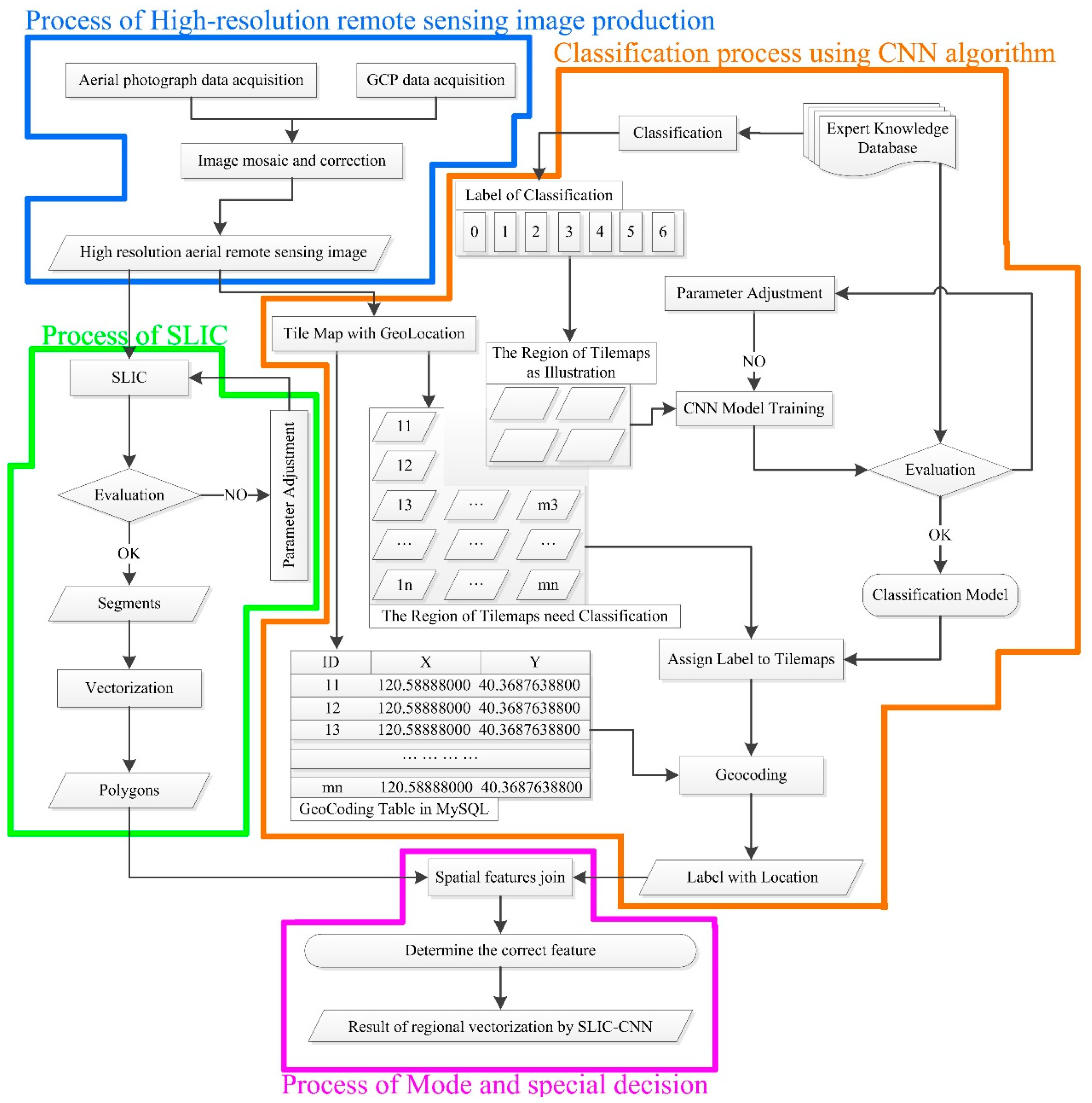
Figure 6.
Parametric schematic diagram of each layer of the AlexNet model.

Figure 7.
Steps of the ordinary deep learning classification process.

Figure 8.
A. Classification result when the Simple Linear Iterative Clustering (SLIC) clustering center step ≈ Convolutional Neural Networks (CNN) slice step length. B. Classification result when the SLIC clustering center step >> CNN slice step size. C. Classification result when the SLIC clustering center step size << CNN slice length.
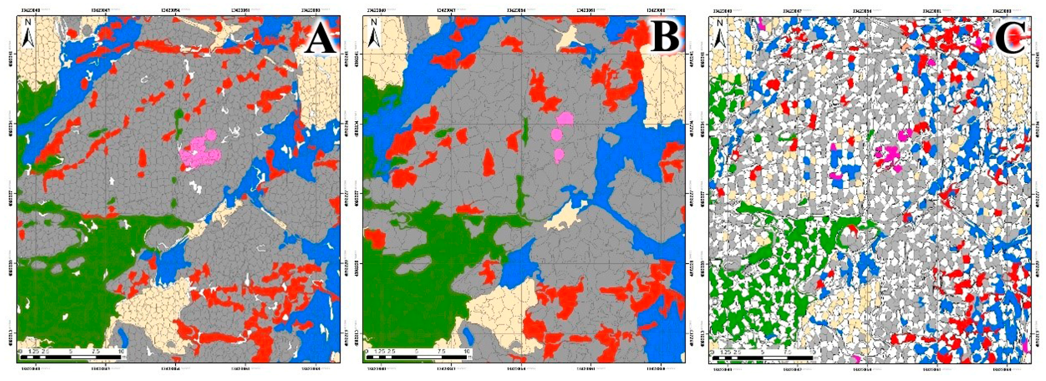
Figure 9.
Segment and CNN correspondence locations of classification points. (A) A segment corresponds to two or more classification points; (B) A segment corresponds to one classification point; and (C) A segment does not have a point that falls within its range.
Figure 9.
Segment and CNN correspondence locations of classification points. (A) A segment corresponds to two or more classification points; (B) A segment corresponds to one classification point; and (C) A segment does not have a point that falls within its range.

Figure 10.
Comparison between the pure CNN classification method and the SLIC-CNN method in the geological mapping process.
Figure 10.
Comparison between the pure CNN classification method and the SLIC-CNN method in the geological mapping process.

Figure 11.
Comparing the calculation time of the CNN model under different parameters in this paper, the horizontal coordinate unit is second, and the ordinate bar name format is “learning rate _batch”.
Figure 11.
Comparing the calculation time of the CNN model under different parameters in this paper, the horizontal coordinate unit is second, and the ordinate bar name format is “learning rate _batch”.

Figure 12.
The 3D surface of average verification rate of the model with several parameters.
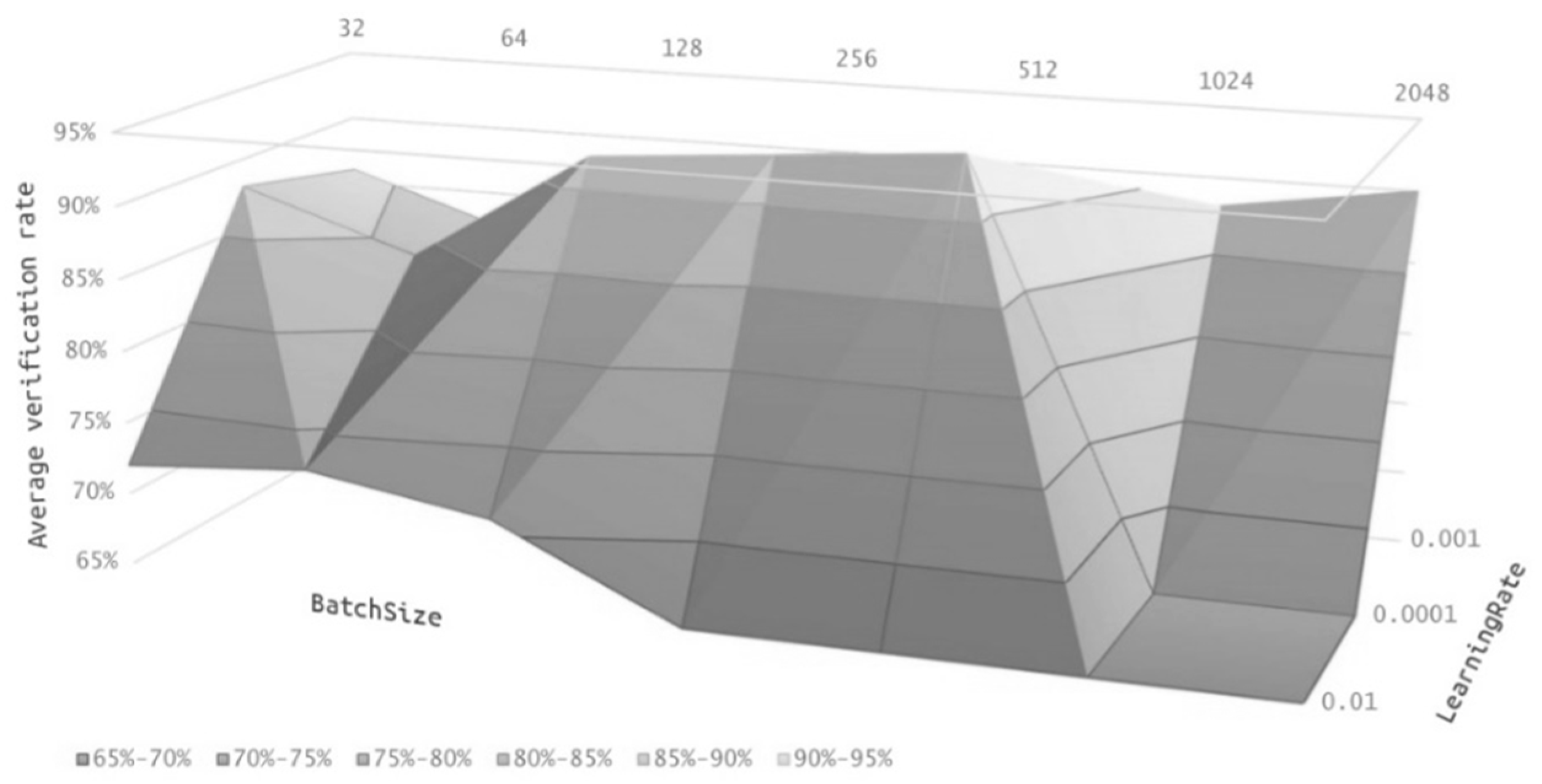
Figure 13.
Accuracy rate curve under different parameters. (a) When the learning rate is 0.001, the model training accuracy rate curve under different parameters 1. (b) When the learning rate is 0.001, the model training accuracy rate curve under different parameters 2. (c) When the learning rate is 0.0001, the model training accuracy rate curve under different parameters. (d) When the learning rate is 0.01, the model training accuracy rate curve under different parameters.

Figure 14.
Verification accuracy rate curve under different parameters. (a) When the learning rate is 0.001, the model verification accuracy rate curve under different parameters 1. (b) When the learning rate is 0.001, the model verification accuracy rate curve under different parameters 2. (c) When the learning rate is 0.0001, the model verification accuracy rate curve under different parameters. (d) When the learning rate is 0.01, the model verification accuracy rate curve under different parameters.

Figure 15.
Simple Linear Iterative Clustering (SLIC) image segmentation results from orthophotos in the study area.
Figure 15.
Simple Linear Iterative Clustering (SLIC) image segmentation results from orthophotos in the study area.

Figure 16.
Comparison of the remote sensing imagery and SLIC-CNN results. (left) Large area remote sensing imagery in the study area. (right) The SLIC-CNN algorithm recognition result.
Figure 16.
Comparison of the remote sensing imagery and SLIC-CNN results. (left) Large area remote sensing imagery in the study area. (right) The SLIC-CNN algorithm recognition result.

Figure 17.
Identification results of three automated classification algorithms for the study areas, (A) Pixel-based classification. (B) Object-oriented classification. (C) AlexNet classification. (D) SLIC-CNN classification.
Figure 17.
Identification results of three automated classification algorithms for the study areas, (A) Pixel-based classification. (B) Object-oriented classification. (C) AlexNet classification. (D) SLIC-CNN classification.

Figure 18.
Receiver Operating Characteristic (ROC) and Area Under The Curve (AUC) of classification result. (a) Standard ROC curve. (b) ROC curve of SLIC-CNN, AlexNet (CNN), pixel-based and object-based method.
Figure 18.
Receiver Operating Characteristic (ROC) and Area Under The Curve (AUC) of classification result. (a) Standard ROC curve. (b) ROC curve of SLIC-CNN, AlexNet (CNN), pixel-based and object-based method.

Figure 19.
(A) SLIC-CNN mapping results. (B) Most detailed geological map of the region from 2004 (1. Orthogneiss. 2. Biotite-bearing granite. 3. Pegmatite. 4, Garnet-bearing granitic aplite. 5. Granitic aplite. 6. Mylonites. 7. Mafic dyke). (C) High-resolution remote sensing images.
Figure 19.
(A) SLIC-CNN mapping results. (B) Most detailed geological map of the region from 2004 (1. Orthogneiss. 2. Biotite-bearing granite. 3. Pegmatite. 4, Garnet-bearing granitic aplite. 5. Granitic aplite. 6. Mylonites. 7. Mafic dyke). (C) High-resolution remote sensing images.

Figure 20.
The large-scale geological map of Taili with SLIC-CNN.


Table 1.
Classification category and quantity.
| Name | Description | Number of Training Samples | Number of Verification Samples | Total Number of Samples |
|---|---|---|---|---|
| Quaternary | Beach, gravel | 600 | 3277 | 3877 |
| Granite Dykes | granite aplite, granite pegmatite | 600 | 281 | 881 |
| Mylonite | Augen mylonites, Augen undeveloped mylonites | 600 | 743 | 1343 |
| Vegetation | Shrubs, grasses, algae, etc. | 600 | 1199 | 1799 |
| Sundries | People, kayaks, lifebuoys, bags, etc. | 30 | 16 | 46 |
| Boardwalk | boardwalk | 600 | 280 | 880 |
| Orthogneiss | Orthogneiss | 600 | 4006 | 4606 |
Table 2.
Pixel-based classification precision confusion matrix.
| Real | Quaternary | Granite Dykes | Mylonite | Vegetation | Sundries | Boardwalk | Orthogneiss | |
|---|---|---|---|---|---|---|---|---|
| Test | ||||||||
| Quaternary | 67.20% | 0.72% | 0.53% | 4.03% | 2.46% | 23.30% | 1.76% | |
| Granite Dykes | 54.10% | 9.27% | 0.07% | 1.93% | 5.62% | 29.01% | ||
| Mylonite | 0.96% | 0.13% | 84.71% | 4.20% | 9.91% | 0.09% | ||
| Vegetation | 0.45% | 0.76% | 0.06% | 88.08% | 0.60% | 4.60% | 5.45% | |
| Sundries | 1.57% | 77.02% | 8.29% | 13.11% | ||||
| Boardwalk | 28.97% | 11.17% | 3.02% | 3.62% | 5.01% | 48.15% | 0.06% | |
| Orthogneiss | 2.42% | 31.55% | 2.41% | 12.97% | 0.13% | 50.52% | ||
Table 3.
Object-oriented classification precision confusion matrix.
| Real | Quaternary | Granite Dykes | Mylonite | Vegetation | Sundries | Boardwalk | Orthogneiss | |
|---|---|---|---|---|---|---|---|---|
| Test | ||||||||
| Quaternary | 45.54% | 1.19% | 2.04% | 24.81% | 2.09% | 21.98% | 2.35% | |
| Granite Dykes | 0.30% | 54.60% | 13.22% | 4.36% | 1.71% | 5.66% | 20.15% | |
| Mylonite | 0.96% | 10.48% | 61.72% | 19.27% | 7.57% | |||
| Vegetation | 20.91% | 0.72% | 6.17% | 48.03% | 15.16% | 4.59% | 4.42% | |
| Sundries | 6.50% | 1.45% | 4.34% | 61.62% | 11.97% | 14.12% | ||
| Boardwalk | 23.76% | 5.86% | 5.53% | 3.40% | 5.27% | 48.06% | 8.12% | |
| Orthogneiss | 2.03% | 25.70% | 6.98% | 0.13% | 14.15% | 0.17% | 50.84% | |
Table 4.
AlexNet classification precision confusion matrix.
| Real | Quaternary | Granite Dykes | Mylonite | Vegetation | Sundries | Boardwalk | Orthogneiss | |
|---|---|---|---|---|---|---|---|---|
| Test | ||||||||
| Quaternary | 93.09% | 2.28% | 2.57% | 5.40% | 3.16% | 1.22% | ||
| Granite Dykes | 0.46% | 53.15% | 5.69% | 0.24% | 0.25% | 6.07% | ||
| Mylonite | 1.03% | 9.86% | 85.79% | 0.59% | 1.02% | 1.54% | ||
| Vegetation | 2.07% | 0.50% | 0.15% | 90.52% | 1.36% | |||
| Sundries | 0.16% | 85.50% | 0.17% | |||||
| Boardwalk | 1.36% | 0.82% | 0.95% | 0.16% | 95.82% | |||
| Orthogneiss | 1.99% | 33.23% | 5.81% | 2.29% | 14.09% | 89.63% | ||
Table 5.
SLIC-CNN classification precision confusion matrix.
| Real | Quaternary | Granite Dykes | Mylonite | Vegetation | Sundries | Boardwalk | Orthogneiss | |
|---|---|---|---|---|---|---|---|---|
| Test | ||||||||
| Quaternary | 93.46% | 1.93% | 2.57% | 5.01% | 1.26% | 1.31% | ||
| Granite Dykes | 0.39% | 54.26% | 4.85% | 0.06% | 5.5% | |||
| Mylonite | 0.67% | 10.28% | 86.96% | 0.46% | 1.58% | |||
| Vegetation | 2.26% | 0.33% | 0.32% | 91.69% | 1.36% | 1.04% | ||
| Sundries | 0.01% | 0.27% | 83.08% | 0.09% | ||||
| Boardwalk | 1.23% | 0.73% | 0.36% | 0.19% | 97.38% | 0.07% | ||
| Orthogneiss | 1.98% | 32.19% | 5.30% | 2.42% | 16.73% | 90.4% | ||
© 2020 by the authors. Licensee MDPI, Basel, Switzerland. This article is an open access article distributed under the terms and conditions of the Creative Commons Attribution (CC BY) license (http://creativecommons.org/licenses/by/4.0/).
Share and Cite
MDPI and ACS Style
Sang, X.; Xue, L.; Ran, X.; Li, X.; Liu, J.; Liu, Z. Intelligent High-Resolution Geological Mapping Based on SLIC-CNN. ISPRS Int. J. Geo-Inf. 2020, 9, 99. https://0-doi-org.brum.beds.ac.uk/10.3390/ijgi9020099
AMA Style
Sang X, Xue L, Ran X, Li X, Liu J, Liu Z. Intelligent High-Resolution Geological Mapping Based on SLIC-CNN. ISPRS International Journal of Geo-Information. 2020; 9(2):99. https://0-doi-org.brum.beds.ac.uk/10.3390/ijgi9020099
Chicago/Turabian StyleSang, Xuejia, Linfu Xue, Xiangjin Ran, Xiaoshun Li, Jiwen Liu, and Zeyu Liu. 2020. "Intelligent High-Resolution Geological Mapping Based on SLIC-CNN" ISPRS International Journal of Geo-Information 9, no. 2: 99. https://0-doi-org.brum.beds.ac.uk/10.3390/ijgi9020099
Note that from the first issue of 2016, this journal uses article numbers instead of page numbers. See further details here.