Indexing Mixed Aperture Icosahedral Hexagonal Discrete Global Grid Systems


PLA Strategic Support Force Information Engineering University, Zhengzhou 450001, China
*
Author to whom correspondence should be addressed.
ISPRS Int. J. Geo-Inf. 2020, 9(3), 171; https://0-doi-org.brum.beds.ac.uk/10.3390/ijgi9030171
Submission received: 22 January 2020
/
Revised: 29 February 2020
/
Accepted: 8 March 2020
/
Published: 13 March 2020
(This article belongs to the Special Issue Global Grid Systems)
Abstract
:Discrete global grid systems (DGGSs) are an emerging multiresolution 3D model used to integrate and analyze big earth data. The characteristic of multiresolution is usually realized by hierarchically subdividing cells on the sphere using certain refinement. This paper introduces mixed aperture three- and four- icosahedral hexagonal DGGSs using two types of refinement, the various combinations of which can provide more resolutions compared with pure aperture hexagonal DGGSs and can flexibly design the aperture sequence according to the target resolutions. A general hierarchy-based indexing method is first designed, and related indexing arithmetics and algorithm are developed based on the indexing method. Then, the grid structure on the surface of the icosahedron is described and by projection spherical grids are obtained. Experiments show that the proposed scheme is superior to pure aperture schemes in choosing grid resolutions and can reduce the data volume by 38.5% in representing 1-km resolution raster dataset; using the proposed indexing arithmetics to replace spherical geometry operations in generating discrete spherical vector lines based on hexagonal cells can improve the generation efficiency.
1. Introduction
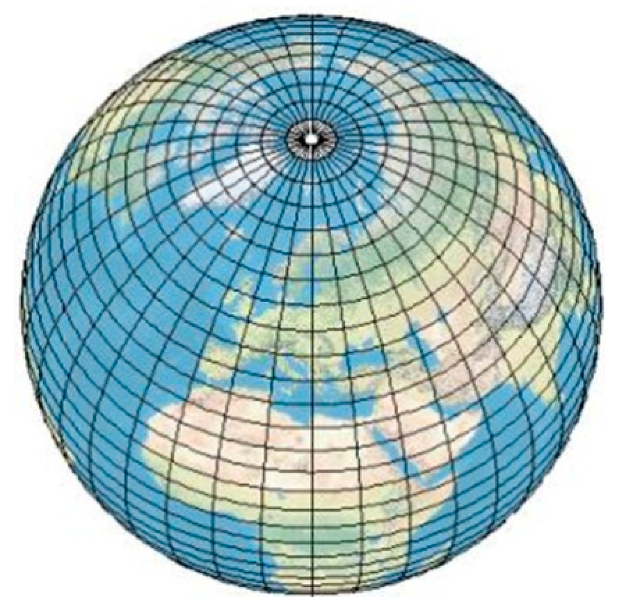
In recent years, the explosive growth of geospatial data volume and the increasingly complicated and multiple data structures have posed a great challenge to their integration and analysis [1]. Traditional two-dimensional (2D) maps based on map projections usually represent local areas of the earth and only provide a flat view of the globe [2]. In addition, location representation using geographical coordinates may cause truncation errors in computers due to the use of floating-point numbers and thus add calculation complexity [3]. The longitude and latitude framework can represent the three-dimensional (3D) globe. However, cells in this framework are usually irregular [2], where the cells will change from the equator to poles with increasing of latitude and at the poles the quadrilateral cells degenerate into triangles [4].
Discrete global grid system (DGGS) is a spatial reference framework being developed to solve the above problems. Under this framework, the earth is discretized into a set of cells. Each cell represents an area on the surface of the earth and all data related to the area can be assigned to the cell, which helps integration of multi-source datasets. DGGS can provide more regular cells to partition the Earth into a multiresolution hierarchy, and the earth is approximated by a regular polyhedron as the initial tessellation [4]. The integer index is assigned to each cell for location representation. Based on these characteristics, DGGSs have aroused widespread academic attention and been developed in various fields, such as global gazetteer [5], ocean tidal simulation [6], and handling big Earth data with cloud computing technology [7]. The Open Geospatial Consortium (OGC) has released an abstract specification for DGGS [8], which highlights equal-area cells desirable in the integrated analysis of very large, multisource, and multiresolution geospatial data. DGGSs differ in basic elements such as the base polyhedron, the type of cells, the type of refinement and the indexing method.
Regular cells used in DGGSs are triangles, quadrilaterals, and hexagons. Among the three shapes, hexagons have a uniform neighboring relationship that can help spatial analysis [4,9]. They also have the highest packing density and best approximate the circular regions [10]. ARCGIS has developed a tool of creating the hexagon tessellation on the 2D plane for statistical analysis due to its good geometric properties [11]. However, unlike triangles and quadrilaterals, hexagons have no congruence that means a big hexagon cannot be composed of several small hexagons, which complicates the multi-resolution application of hexagons.
The realization of multiresolution for a DGGS is through refinement of cells from the coarse resolution to a fine resolution. For example, the common refinement for quads is 1-to-4. Amiri et al. proposed a 1-to-2 refinement quadrilateral DGGS based on a cube and obtained a smoother transition among cells [12]. This scheme can also provide more resolutions in a finite resolution range, which is desirable in data representation because there are more possibilities that we can choose a grid resolution closest or equal to the target resolution to maintain the authenticity of data and reduce data volume. In addition to the smaller ratio of refinement, a combination of different types of refinement is another method to approach the target resolution as much as possible. Refinement is also called aperture. Apertures for hexagonal DGGS are aperture 3, 4, and 7 [3]. However, current hexagonal DGGSs are mainly based on the pure aperture sequence and restrict the resolutions for application. Sahr proposed a general scheme for the mixed aperture hexagonal DGGS named Central Place Indexing (CPI) [13]. CPI is applicable to the mixed sequence of aperture 3, 4, and 7, and the aperture sequence can be designed according to target resolutions, which is obviously a more flexible scheme than those based on pure apertures.
DGGSs should be able to visualize, integrate, and analyze various geospatial datasets [2,14]. To assign the data into associated cells, an indexing method is necessary for data querying. Indexing arithmetics also need to be defined for geospatial analysis such as neighboring finding and distance measurement. Hierarchy-based indexing methods have extremely high efficiency in hierarchical traversal. A hierarchical index can not only embody location information but also reflect the cell resolution, thus there is no need for metadata [13]. Since hexagons have no congruence, the hierarchical relationship for hexagonal cells is not as simple and clear as that for triangular and quads; therefore researchers have studied and proposed different hierarchy-based indexing methods for hexagonal DGGSs [10,15,16,17]. Current hierarchy-based indexing methods and related indexing algorithms are mainly focused on pure aperture hexagonal DGGSs and cannot be applied to mixed aperture ones. CPI defines a general indexing method for different mixed aperture sequences, but it involves less about specific indexing arithmetics and algorithms.
This paper focuses on mixed aperture 3 and 4 hexagonal DGGSs and proposes a hierarchy-based indexing method based on cell directions. The general arithmetic rule and algorithm are also given for all mixed aperture 3 and 4 sequences. To verify the availability and efficiency of our scheme, this paper represents the current global raster dataset, uses current vector data to generate discrete spherical vector lines, and respectively compares the data volume used and number of cells in vector lines generated in unit time between the proposed scheme and other existing schemes.
We organize the paper as follows: related work is presented in Section 2. Section 3 describes the proposed scheme for the mixed aperture 3 and 4 hexagonal DGGS. The proposed indexing method for the mixed aperture 3 and 4 hexagonal grid and related indexing arithmetics and algorithm are first described. Then, the grid on the surface of the icosahedron and projection into the sphere is discussed. In Section 4, global raster datasets and vector data are applied in our scheme, and comparisons with other schemes are given. Conclusions and future work are presented in Section 5.
2. Related Work
A DGGS reference framework should consist of the following core elements: base polyhedron, type of cells, tessellation, and type of index [12].
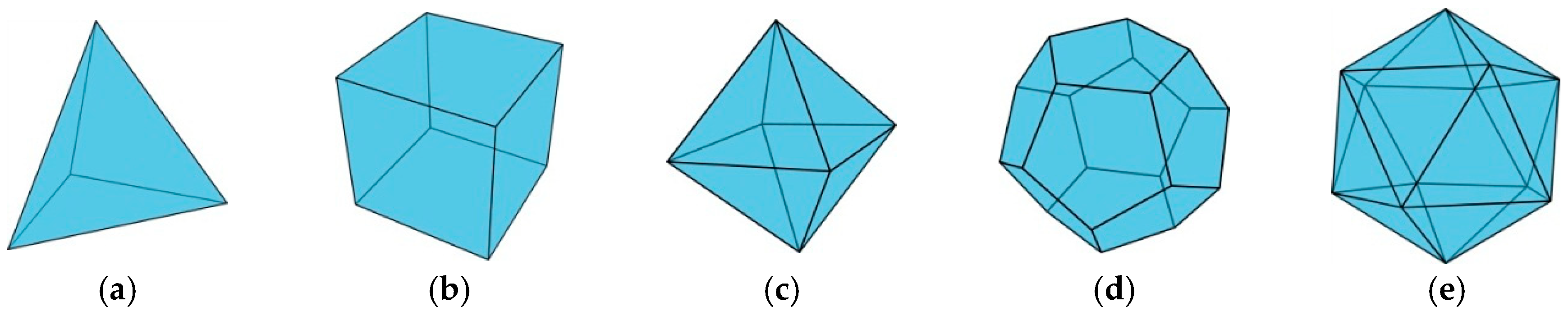
Base polyhedron: There are five regular polyhedrons used in DGGSs, which are tetrahedrons, cubes, octahedrons, dodecahedrons, and icosahedrons (Figure 1).
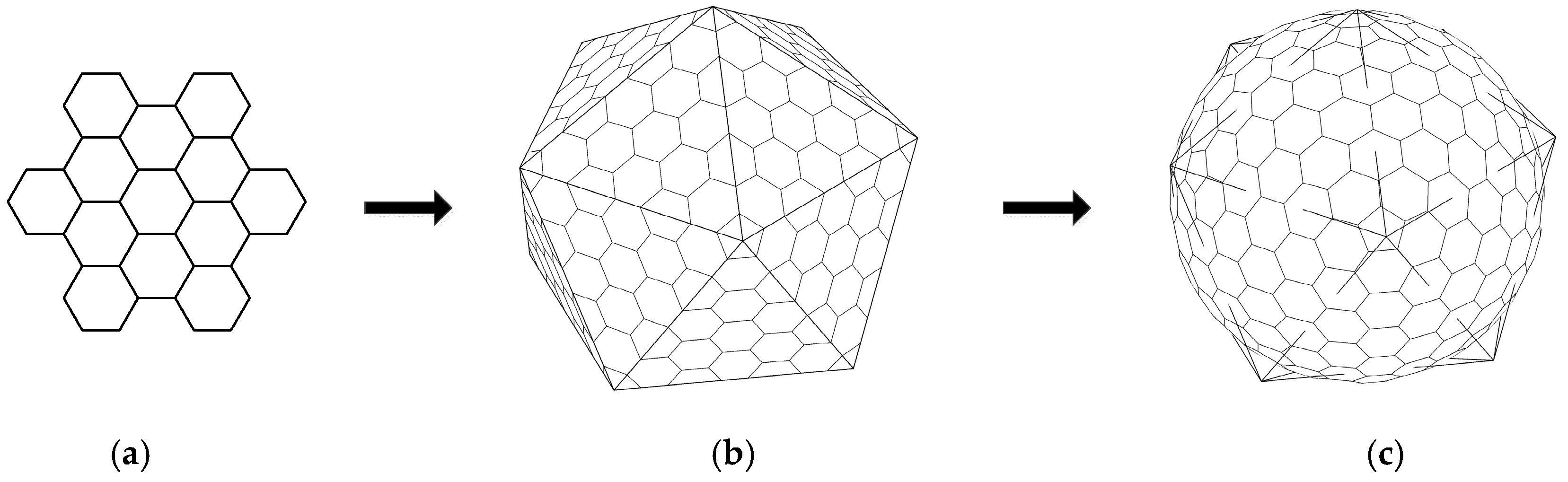
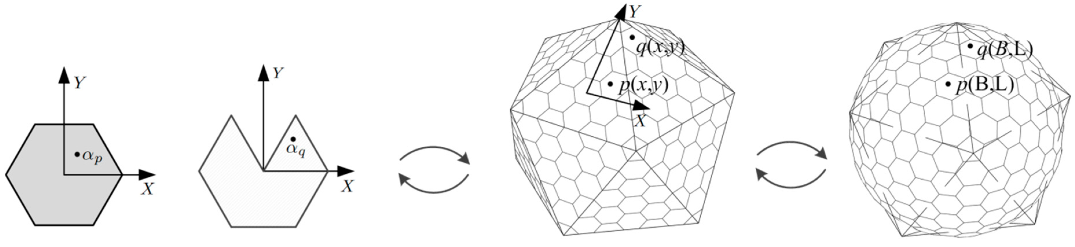
The tetrahedron is simple and it was ever used to construct the virtual globe [18]. DGGSs based on cubes are popular [12,19,20]. Cubes can fit the Cartesian coordinate system well, which facilitates calculation. The octahedron has a relatively simple location relation with the earth [4,21]. Bai et al. and Ben et al. have studied the hexagonal DGGSs based on an octahedron about hierarchical partitioning, indexing, and grid generation [21,22]. The dodecahedron is used less often due to its pentagonal faces. The distortion of grid cells in DGGSs based on an icosahedron is the smallest because faces of the icosahedron are the most [23]. All faces of the icosahedron are triangles and can be covered by hexagons without overlap and gap (except 12 pentagons centered at 12 vertices of the icosahedron). Currently, most hexagonal DGGSs use an icosahedron as the base polyhedron. The general idea used to construct the icosahedral hexagonal DGGS is illustrated in Figure 2. The idea is to first study the properties of hexagonal grid systems on the infinite plane, then build the hexagonal grid system on the closed surface of the icosahedron, and finally project the icosahedral hexagonal grid system to the sphere. In this paper, an icosahedron is used as the base polyhedron for our proposed scheme.
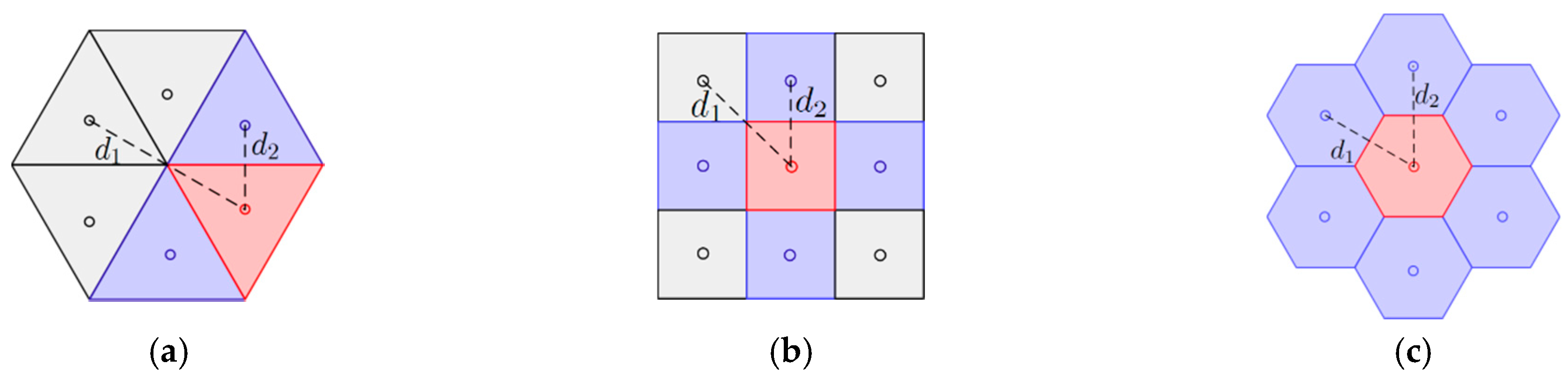
Types of cells: Triangles, hexagons and quadrilaterals are commonly used in DGGSs. Since the faces of most regular polyhedrons are triangles, it is natural to use triangular cells to partition these faces. However, the neighboring relationship for triangles is complicated, as Figure 3a illustrates. It is the same as quads (Figure 3b), but quads can be compatible with most of the current datasets, hardware, and algorithms [12]. The six distances from one hexagonal cell to its six neighbors are identical (Figure 3c), thus hexagons have uniform adjacency which is desirable for spatial analysis in GIS [4]. In addition, relevant research has proven that hexagons have the highest sampling efficiency and angular resolution [9]. In this paper, our scheme chooses hexagons as the base cell.
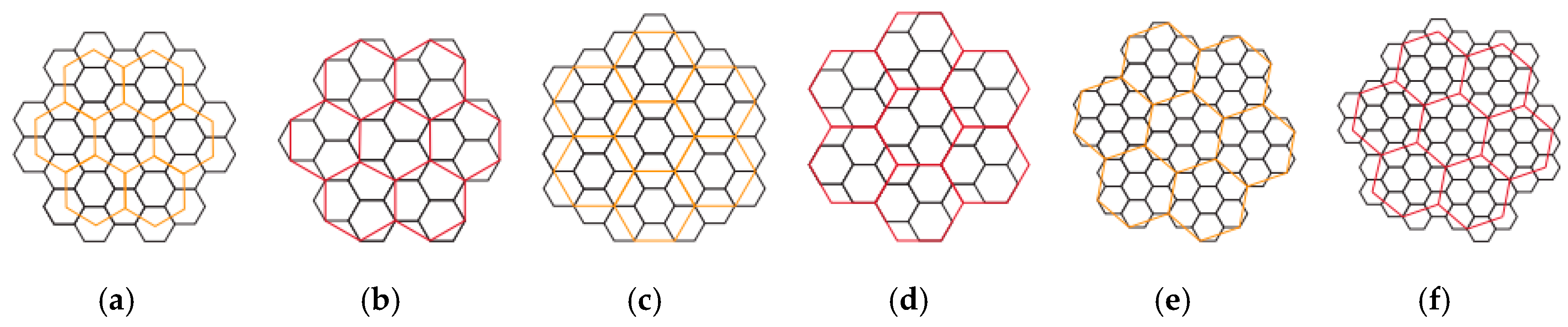
Tessellation: Tessellation involves cell refinement and cell alignment. Refinement is also called aperture. Aperture n means that the area of the fine cells in the next level is that of the coarse cells. The types of aperture for hexagonal grids are 3, 4, and 7. There are two types of cell alignment for hexagons, centroid alignment, and vertex alignment. The former means that the centers of the fine cells are the same as those of the coarse cells and this type is used most often because it is easier to build the hierarchical relationship of cells and more regular. The latter means the coarse cell shares its center with the vertices of finer cells partitioned from it. Figure 4 is cited from the literature [24], and illustrates six types of hexagonal tessellation related to the three apertures for two alignments. Many hexagonal DGGSs use the types in Figure 4a or Figure 4c due to the smoother transition among resolutions and more regular cell assignments on the polyhedron, compared with aperture 7 [10,15,16,17,25]. Uber uses the type in Figure 4e to develop an aperture 7 hexagonal DGGS to study the rules of taxi tracks to improve taxi dispatching and releases H3’s library online [26]. However, hexagonal DGGSs using just one type of aperture are less flexible as discussed in Section 1. In this paper, we use a mix of aperture 3 and 4 with centroid alignment.
Types of index: In a DGGS, each cell is assigned a unique index as a representation of locations, and operations of cells are usually performed through indexing arithmetics. Therefore, the characteristics and arithmetic rules of indices impact the efficiency and reliability of data processing in a DGGS and are the core factors for a DGGS. For aperture 3 hexagonal DGGSs, Vince proposed the barycentric indexing method using an octahedron [27]. Vince also proposed the radix indexing based on an icosahedron. PYXIS is an aperture 3 icosahedral hexagonal DGGS and has been successfully applied in an online-service system for geospatial data called Global Grid Systems by the PYXIS inonovation inc [28]. The indexing arithmetics of this method are complicated because of its fractal coverage hierarchy [24]. Sahr proposed two indexing methods in [15], pyramid indexing and path indexing. The pyramid indexing method is mainly applicable to single resolution. Path indexing is a hierarchy-based indexing method and is similar to that of PYXIS. For aperture 4 hexagonal DGGSs, Tong et al. proposed the hexagonal quad balanced structure (HQBS) [16], but this method indexes centers and vertices of hexagonal cells at the same time, which leads to complicated indexing arithmetic rule and possible failure of operation [29]. Wang et al. proposed the hexagonal lattice quad tree (HLQT) based on a symmetric assignment of aperture 4 child cells [17]. The above are all designed for the pure aperture based on one specific type of polyhedron. Amiri used a coordinate system and designs a general indexing method that is independent of the base polyhedron and aperture [24].
The existing indexing method for mixed aperture hexagonal DGGSs that can be found in the literature is CPI [3,13]. CPI uses the base digits {0,1,2,3,4,5,6} to index hierarchical cells and the assignment of digits is the same as generalized balanced ternary (GBT). CPI also gives the realization of unique index. As discussed earlier, CPI focuses on the general concepts and construction of the mixed aperture hexagonal DGGSs. In this paper, our indexing method is partly developed from CPI because of the use of unique index, but considers cell directions on the 2D plane to define basic digits to simplify operations. We also discuss the indexing arithmetics and algorithms of our scheme in detail.
3. Framework
From the above discussion, the spatial reference framework in our proposed scheme uses an icosahedron as the base polyhedron, combines two types of apertures and designs a hierarchy-based indexing method to construct a hexagonal DGGS. In this paper, we choose aperture 3 and 4 rather than all three types because the combinations of aperture 3, 4, and 7 will generate many possible cell directions led by degrees change in cell direction from aperture 7, which brings great difficulty in exploring the specific rules of indexing arithmetics suitable for all mixed aperture sequences. We initially study mixed aperture 3 and 4, which changes more regularly and our research findings can be a basis of further research on the mixed aperture 3, 4, and 7.
The characteristics of the mixed aperture 3 and 4 grid are first described. Then, the indexing method is proposed, and the indexing arithmetic rules and related algorithm are given. Finally, the mixed aperture 3 and 4 grid on the surface of the icosahedron and projection onto the sphere is introduced.
3.1. Mixed Aperture 3 and 4
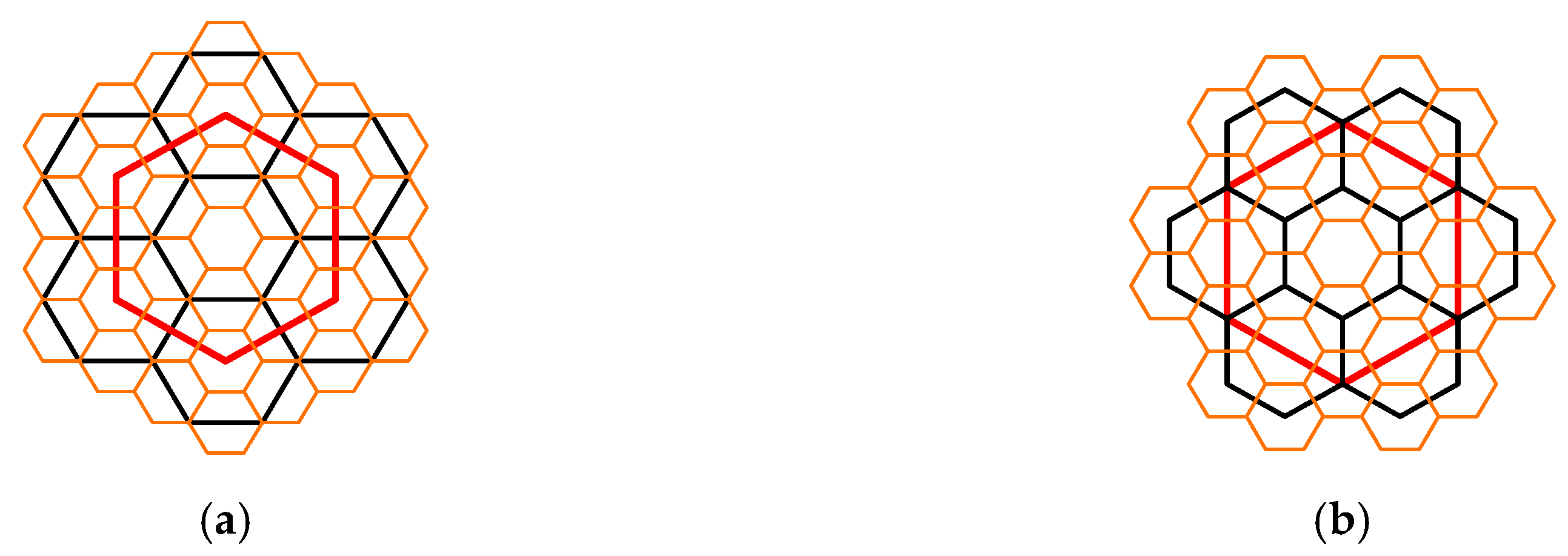
For aperture 3, the area of the finer cells is that of coarse cells and the cell direction changes by 30 degrees. The rotation of cell direction can be counterclockwise or clockwise, but the finer cells obtained are identical. For aperture 4, the area of the finer cells is that of coarse cells and the cell direction remains unchanged. Figure 5 illustrates two basic mixed aperture sequences. In Figure 5a, the aperture sequence is 34. After the refinement of the two apertures, the cell area at level 2 is that at level 0 and the cell direction changes by 30 degrees. In Figure 5b, the aperture sequence is 43 but it can be seen that the area and direction of cells at level 2 are the same as those of Figure 5a. The area and direction of the finest cells have nothing to do with the specific aperture sequence but the number of each aperture.
Assume that the aperture sequence of a mixed aperture 3 and 4 hexagonal grid with levels is , where aperture is 3 or 4, and the numbers of aperture 3 and 4 are and , respectively. Assume the length and the area of cells at level 0 are and , respectively, and use and to denote the length and the area of cells at level , respectively, whichcan be obtained by
3.2. Indexing
3.2.1. Indexing Method
The hierarchical relationship of cells needs to be determined to design a hierarchy-based indexing method. The coarse cell and the finer cells partitioned from it are called the parent cell and the child cells of the parent cell, respectively. The index of a child cell is comprised of the index of its parent cell as the prefix and a digit attached to describe its location related to the parent cell.
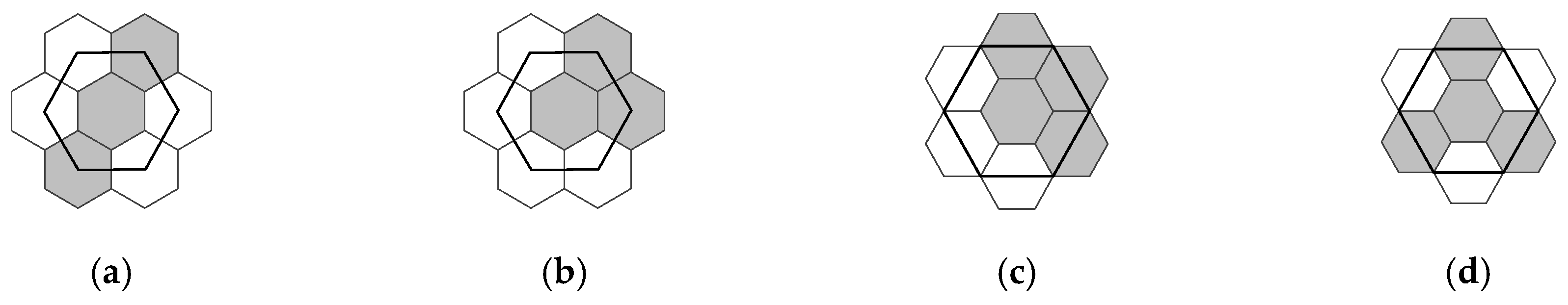
As shown in Figure 5, the hexagons at level 1 can have at most seven child cells at level 2 and may result in multiple indices for a cell at level 2. In a DGGS, each cell has one unique index. To realize the uniqueness of index, each parent cell in one level can generate three child cells for aperture 3 and four child cells for aperture 4 to ensure that the area sum of their children cells is the same as that of the parent cell, and the generated finer cells do not overlap and do not have gaps [13]. Figure 6 illustrates the possible types of child cells chosen from the seven related finer cells for a parent cell, in which the gray cells are the chosen child cells and the white finer cells are the child cells of other parent cells. It can be seen that all types must contain the child cell that shares the center with the parent cell.
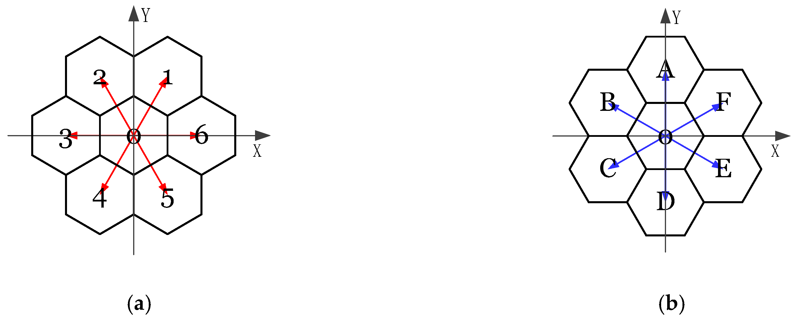
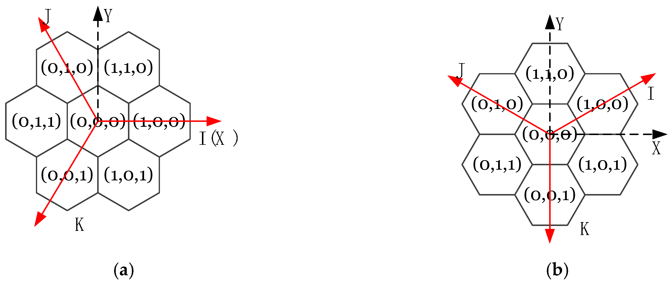
To realize the projection from/to the faces of an icosahedron to/from the sphere, we often need to calculate the 2D Cartesian coordinates of cells on the triangular faces of the icosahedron. After defining a 2D Cartesian coordinate system on the planar hexagonal grid, it can be found that only two classes of cell directions exist for the mixed aperture 3 and 4 hexagonal grids according to the rotation characteristics of aperture 3 and 4. Figure 7a illustrates the first type of cell direction, and the locations of the seven cells can denote seven basic vectors from the center of any parent cell in the last level to the centers of its possible child cells. {0,1,2,3,4,5,6} are the basic digits used to attach to the index of the parent cell to obtain the indices of child cells. Similarly, Figure 7b shows the other type of cell direction, and it has another six vectors different from those in Figure 7a. The hexadecimal numbers {A,B,C,D,E,F} are used as the basic digits, and digit 0 represents zero vector in both classes. This indexing method combines the cell directions on the 2D Cartesian coordinate system to define the basic index digits, which is convenient for obtaining information about the grid from the index and calculating the associated 2D Cartesian coordinates of this index.
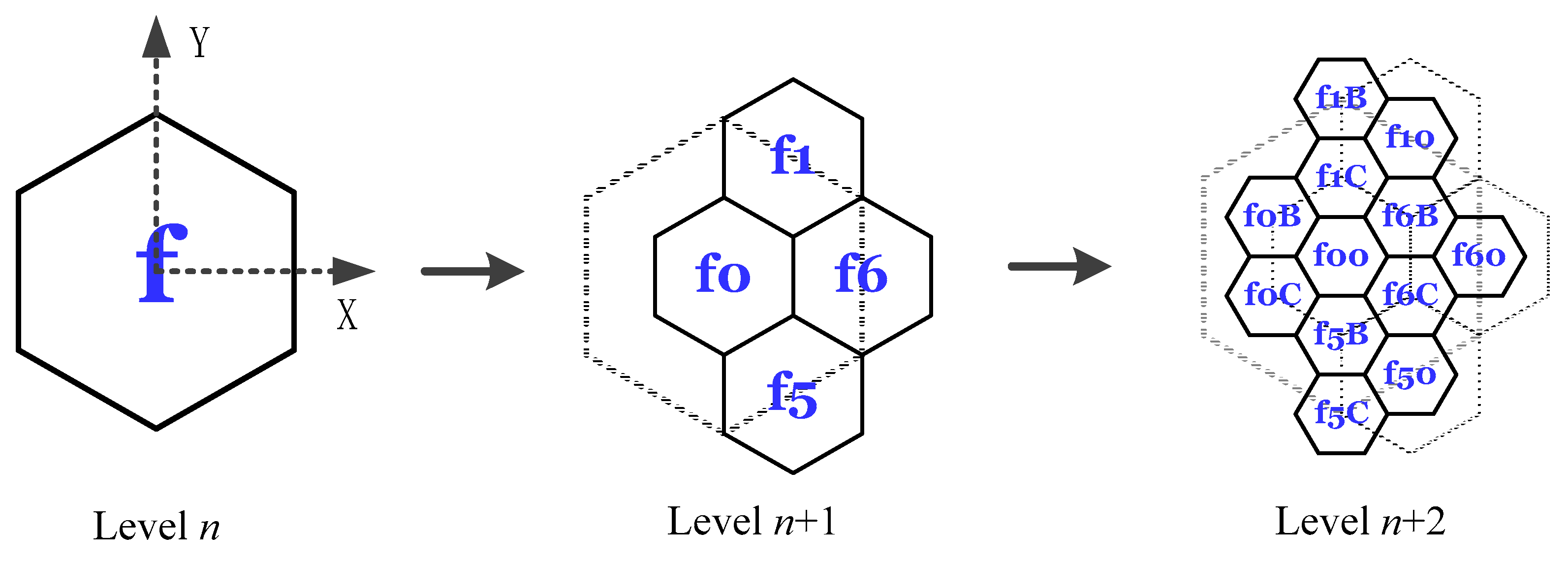
Figure 8 is an illustration of our proposed indexing method. Assume the index of one cell at level is f and the aperture sequence from level to is 43. If the origin of the 2D Cartesian coordinate system is translated into the center of the cell f, the relationship between the two axes and this cell is as Figure 8 shows. To make each index unique, the types from Figure 6c and Figure 6b are chosen for aperture 4 and 3, respectively, to generate child cells at the two subsequent levels. The digit set of the chosen child cells for aperture 4 is {0,1,5,6} and that for aperture 3 is {0, B,C}. It needs to be noted that in addition to {0,1,5,6}, the digit sets Figure 6c represents could also be {0,4,5,6}, {0,1,2,6}, etc.
Above all, the set representing the whole index digits in our proposed method includes 13 basic digits; that is, . If we use the locations of the centers of the hexagonal cells to represent the locations of the cells on the plane, these digits represent 13 basic 2D vectors, whose lengths are dependent on the specific grid level and aperture sequence. To calculate the 2D coordinates of one cell, only the related basic vector for each digit of its index in each level and the vectors of the initial parent cell at level 0 need to be added. Hereinafter, the indices represent the locations of the centers of the hexagonal cells.
3.2.2. Indexing Arithmetics and Algorithms
As discussed earlier, indices are just the one-dimensional (1D) integer representations of the 2D floating-point coordinates of cells on the plane; therefore, indexing arithmetics correspond to 2D vector arithmetics [30], which can improve the calculation efficiency because integers are more suitable for computers to process. The most important and essential indexing arithmetic is index addition for most spatial analyses are realized based on it, such as neighborhood queries and buffering analyses. Index subtraction is just the inverse operation of addition [30]. In this section, we introduce indexing addition of our proposed indexing method.
Use to denote index addition. Assume two indices at level : and where and and are the digits indexing the initial cells at level 0, which can be defined by the practical situation. Let . Index addition works similar to decimal addition starting from the right digit position of level to the left digit position of level 0. Thus, is calculated first. Addition tables are used to obtain the addition result quickly in the computer implementation. Table 1a, and b are addition tables for digits of aperture 3 and aperture 4, respectively, where the first row and the left column are digits related to the chosen type of child cells, and obviously, . For example, assume the aperture from level to level is 3 and the digit set associated with chosen generated cells is ; that is, similar to that for level (Figure 8). If and , according to Table 1a, and are the possible carries for all the left digit positions. If the last carry digit in is , the result of at digit position will be obtained by calculating .
From Table 1, digit added to any digit produces no carry digit for the left positions because digit is actually a zero vector. Index addition is commutative: . There exist general rules to find the result digit in the digit position being calculated, which has nothing to do with the specific mixed aperture sequences, but carry digits such as produced for the left digit positions are related to the specific aperture sequence and the chosen types of child cells in each level.
To complete index addition, carry digits such as , and in Table 1a need to be obtained. Assuming the initial cell centered at the origin of the 2D Cartesian coordinate system at level 0 is indexed by 0, the index of the cell centered at the origin at level must be , whose child cells at level are , , and if the aperture is 3 and the digit set is . Let , ; it can be found that the carry digits produced by are just . Therefore, we need to calculate all to obtain the carry digits for addition at the digit position for level and calculate that from level 1 to level if the grid has levels. Since there is no direct rule to know the carry digits for different aperture sequences and types of child cells, a general algorithm is utilized to obtain them and the complete addition tables before implementing index addition.
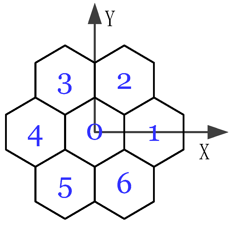
This algorithm of obtaining carry digits for index addition uses the IJK coordinate system, which has three natural axes and uses 3D integer coordinates for location representation [19]. The IJK coordinate system rotates with the cell direction; therefore, it needs to distinguish between clockwise and counterclockwise rotation of aperture 3. In our scheme, we define the IJK coordinate system according to cell directions (Figure 9) to ensure that each digit in set corresponds to one fixed . For example, digit 1 corresponds to . Therefore, it is easy to calculate the coordinates that , , represents.
Let function denote the related coordinate of digit ; the specific steps to calculate are as follows:
(1) Calculate at level ; the result is denoted by ;
(2) Convert to its corresponding index ; is just equal to . Thus, can be obtained.
(3) Repeat steps (1) and (2) to calculate all possible at all levels, and complete addition tables are obtained.
For the conversion from to the hierarchy-based integer index, Sahr proposed an algorithm for the CPI method in the literature [31], and we can adjust the corresponding digit of the coordinates according to our indexing method and Figure 9 based on this algorithm.
It needs to be clarified that our method of index addition is different from that of CPI. The indexing addition for CPI is first to convert the two indices into coordinates, then to add the two coordinates, and finally to convert the resulting coordinate to the index [31]. This method requires multiple conversions and the indices do not participate in the addition operation directly because the addition is not actually realized by operation of digits of index. In the proposed indexing addition algorithm, coordinates are just used to obtain the addition tables, and then the tables are stored in computers before implementing index addition. The coordinates are not involved in the process of index addition, which can have higher efficiency than the CPI algorithm.
Appendix A gives an example of addition tables obtained by the above proposed method and an example of index addition.
3.3. Grid on the Surface of the Icosahedron and Projection
As Figure 2 shows, hexagonal grid systems are usually built on the surface of an icosahedron first and then projected onto the sphere to obtain the hexagonal DGGS as the planar grids cannot be placed directly on the sphere, which will cause the grids to break. The faces of the polyhedron can be seen as planes so that we can easily partition the grids on them; then, the polyhedral hexagonal grids can be projected onto the sphere by projections. The topological relationship between cells also remains unchanged; thus, the result of indexing addition remains the same.
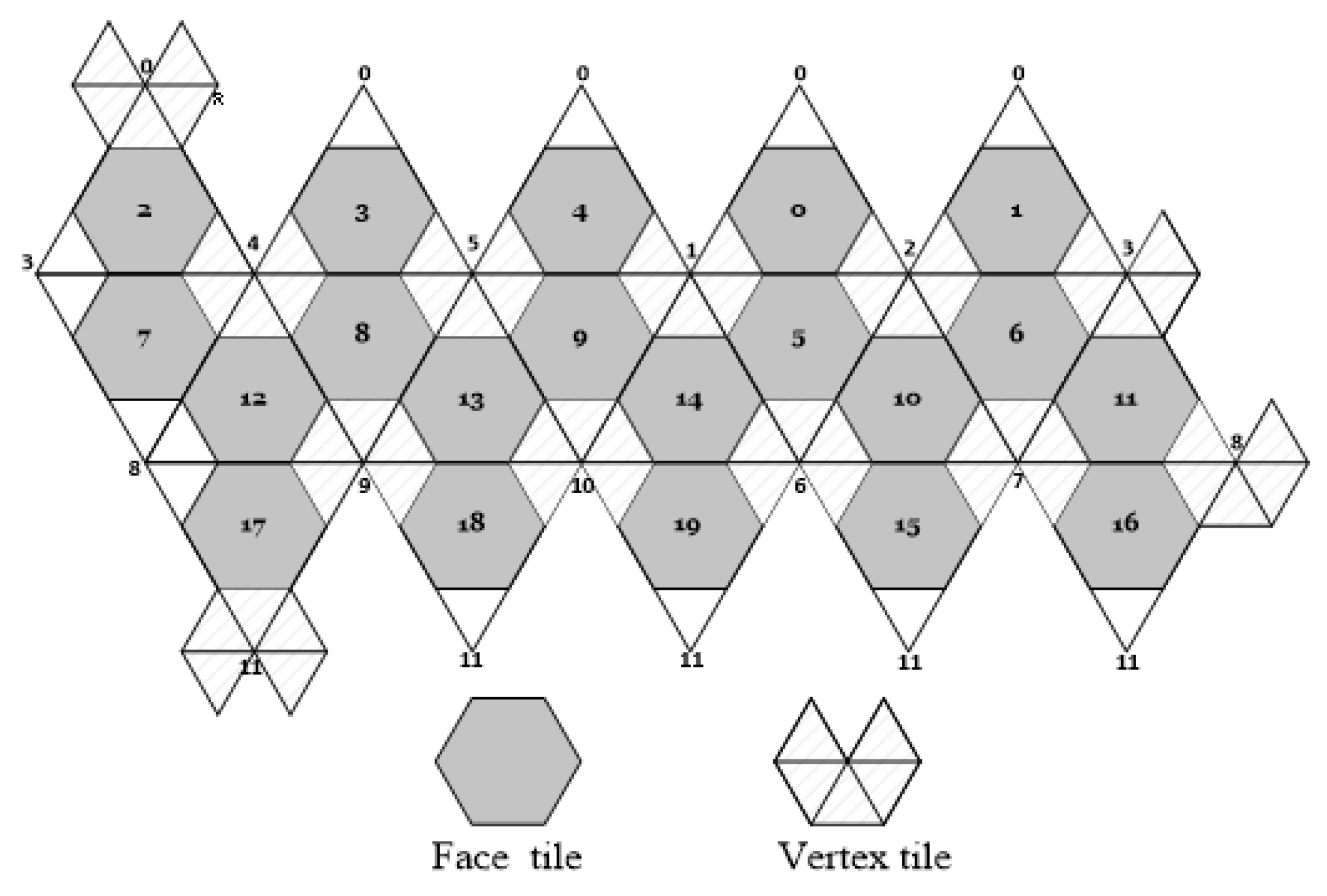
Vince utilized characteristics of natural fractal coverage of aperture 3 hexagonal grids and designed two types of grid tiles to form the icosahedral aperture 3 hexagonal grid system [10]. However, the mixed aperture 3 and 4 hexagonal grid has no such natural structure as aperture 3 does because the generated grids and their boundaries vary with the change of aperture sequences and types of child cells. To build an icosahedral hexagonal grid structure suitable for all mixed aperture sequences, we also design two types of tiles, which are distinguished by boundaries, as Figure 10 illustrates. One type uses as boundaries the edges of hexagons filled in gray and centered at 20 triangular faces of the icosahedron, and the set of cells inside them are called face tiles as well. The other type is the vertex tiles using area filled in white and centered at 12 vertices of the icosahedron as boundaries and the area of each vertex tile is composed of five small triangles, which are unfolded from a pentagon.
To simplify the operations, the 20 hexagons and 12 pentagons are used as the initial cell. In the subsequent partition, we restrict the generated grid inside the boundaries of each tile, which are the edges of the hexagon and pentagon respectively. Therefore, the number and assignment of the generated cells in each tile are not related with the specific aperture sequence.
To obtain equal-area cells, in this paper, the Snyder equal-area polyhedral projection is used to project the icosahedral hexagonal grid onto the sphere. This projection takes the center of each face of the polyhedron as the projection center and defines a forward and inverse projection, where the forward projection is from the sphere to the plane and the inverse projection is from the plane to the sphere [32]. According to this projection and our proposed scheme, we can design the conversion between indices and geographical coordinates to promote interoperability between DGGSs and current datasets based on geographical coordinates. Figure 11 gives the diagram of the conversion. The process from to index first uses the forward projection to the 2D coordinate on a single triangular face, then transforms into the coordinate on a single tile and finally obtains the index using the conversion from coordinate to index. The process from index to is just inverse.
4. Experiments and Discussion
Two experiments are presented to verify the advantages of our proposed scheme. A DGGS should support both raster datasets such as images or elevation datasets, and vector data. In the first experiment, we compare the data volume different schemes use to represent the raster dataset. In the second experiment, the discrete vector line using hexagonal grids is generated based on the index arithmetics we propose in Section 3 and we compare the generation efficiency, which is measured by number of cells generated in unit time, with that of the traditional algorithm.
4.1. Mixed Aperture Hexagonal Representation of a Global Raster Dataset
Most current global geospatial raster datasets are designed based on geographic coordinates and their sampling cells are usually quadrilaterals. For example, the global digital elevation model (DEM) GTOPO30 that will be used in our first experiment is sampled using quadrilateral cells with uniformly-spaced latitudes and longitudes as illustrated in Figure 12. The GTOPO30 dataset can be downloaded from [33]. The arc interval of cells in GTOPO30 are 30-arc seconds, therefore the dataset has dimensions of 21,600 rows and 43,200 columns and a total of 9.3312×10⁸ cells. This geographical framework cannot provide equal–area cells. With increasing latitude, the area of cells will gradually decrease, and the degree of data redundancy will increase as well if the dataset are designed for one resolution. The GTOPO30 dataset is designed for approximately 1 km resolution, but actually only the lengths of cells located at the equator are approximately 1 km, which will certainly cause data redundancy and the degree of redundancy increases with latitude increase. In this experiment, the proposed mixed aperture 3 and 4 icosahedral Snyder equal-area hexagonal grid system is used to represent the GTOPO30 dataset, the data volume using different schemes is compared and the results are shown.
The specific steps for representing GTOPO30 in the proposed scheme are as follows:
(1) Comparison with existing pure aperture hexagonal DGGS to specify the grid level and the aperture sequence;
To integrate one dataset into the DGGS, one appropriate grid level should be determined first: The resolution of GTOPO30 is about 1 km, which can be considered that the length of cell is approximately 1 km or the area of the cell is approximately 1 km2 in that the cell is quadrilateral (except cells at the poles). According to the equal-area characteristic of our proposed scheme, the cell area 1 km2 is taken as the indicator. Assume the number of cells in one grid resolution is , the spherical area is km2, and the area of hexagonal cells is km2. It should be noted that the 12 pentagons centered at the 12 vertices of the icosahedron exist for any level of the icosahedral hexagonal DGGS and their area is exactly five-sixths that of the hexagonal cells at the same level. Therefore, the area of the hexagonal cells is
In this paper, the earth’s radius is chosen as 6371.007180918475 km, which is the WGS84 authalic sphere radius. Table 2 gives the information about the chosen grid levels based on the indicator. Apart from the proposed scheme, we also provide the chosen grid levels in three similar equal-area hexagonal DGGSs, which are pure aperture 3, aperture 4, and aperture 7 hexagonal DGGS, where the statistics of aperture 7 is based on H3 [26]. The three systems all use icosahedron as the base polyhedron and Snyder equal-area polyhedral projection. Table 2 gives the grid level, aperture sequence, number of cells and cell area for different schemes to determine one grid resolution that is most suitable for the indicator. The pure aperture schemes just have one aperture thus we do not give the aperture sequence.
From Table 2, the level determined for the proposed scheme is 16. The final cell resolution of the hexagonal grid systems has nothing to do with the specific aperture sequence and is just associated with the number of each aperture as discussed in Section 3.1. Hence, we just need to know the number of aperture 4 or aperture 3. The number of aperture 4 in the 16 grid levels should be 1 and the number of aperture 3 is obviously 15. Comparing cell areas in the four schemes, our scheme is nearest to the indicator 1 km2. It is because the number of resolutions for the hexagonal DGGS using just one type of aperture is much smaller than mixed aperture and cannot adjust according to the target resolution. However, the mixed aperture hexagonal DGGS has more flexibility and can produce a combination of apertures to match the target resolution as much as possible.
It is obvious that the mixed aperture 3 and 4 scheme should be chosen from the aspect of cell resolution. To further compare the data volume our scheme uses with the original data volume GTOPO30 uses, it just needs to compare the number of cells to cover the surface of the earth. Table 3 gives the comparison results. It can be seen that using the proposed scheme can save 38.5% of the data volume for representing the global elevation model.
Note that if other datasets with the same resolution as GTOPO30 are resampled, the same comparison results that Table 2 and Table 3 present can be obtained. It can also be concluded that if datasets based on the longitude and latitude framework with different resolutions are used, the proposed scheme can also save data volume due to its properties.
(2) GTOPO30 data resampling based on the proposed scheme;
After determining the grid level, we resample the GTOPO30 dataset into it. This experiment uses the indirect resampling method where the calculation is from each index of generated hexagonal grids to the pixel of the original DEM to avoid irregular situations. The specific steps are as follows:
- Generate the grid of the chosen level and calculate the geographic coordinate of the center of each cell;
- Convert from the location of the center of each cell to the row and the column of the pixel the center located in the DEM dataset;
- Give the elevation value of this pixel to this hexagonal (or pentagonal) cell as the elevation of the area this cell represents.
In addition to GTOPO30, other raster datasets can also be resampled using similar steps. The coordinate conversion between the coordinate system the dataset used and the indices of the proposed method should be specified.
(3) Experimental Results
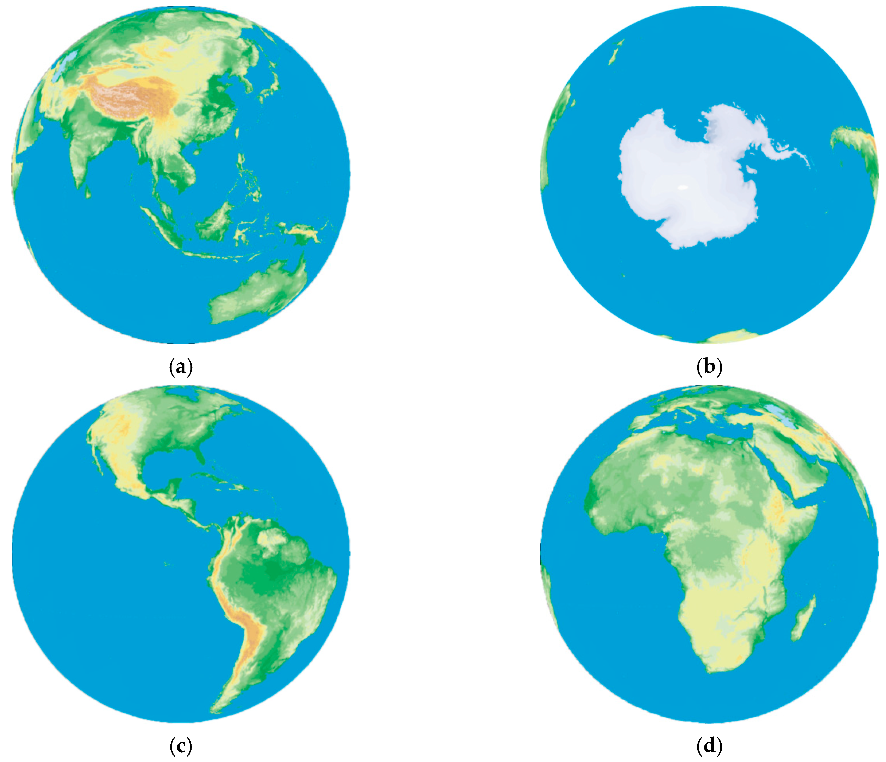
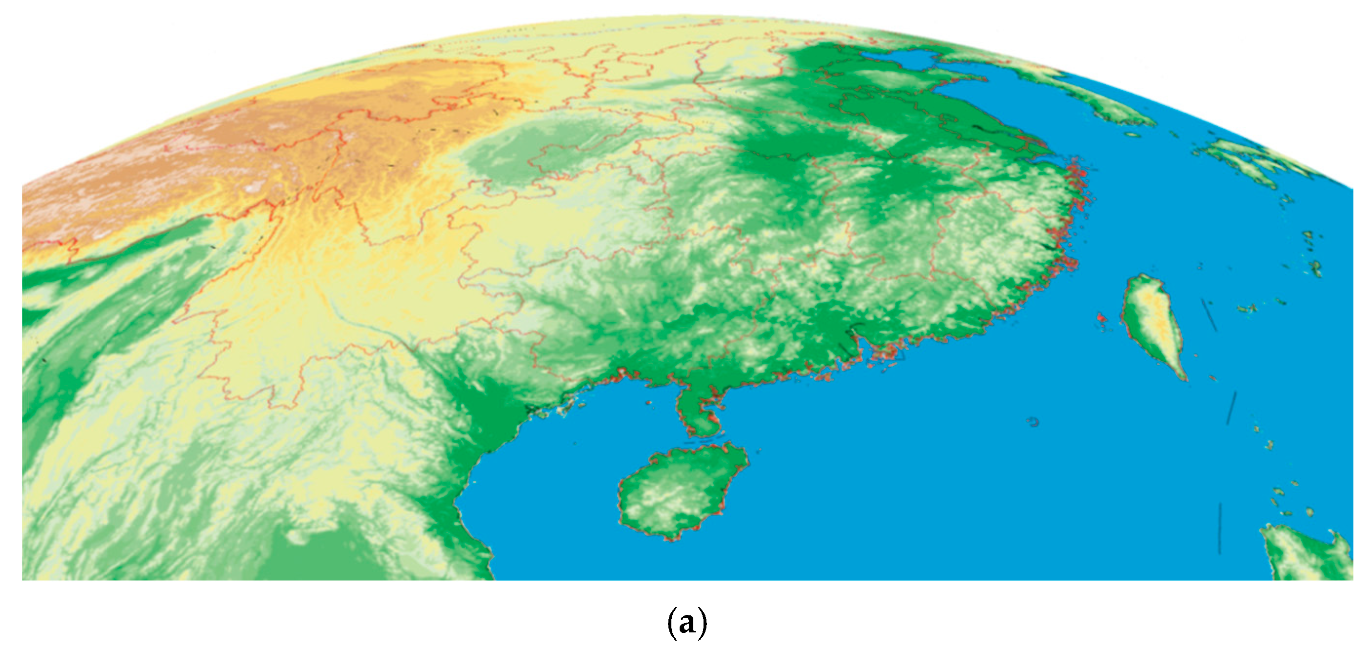
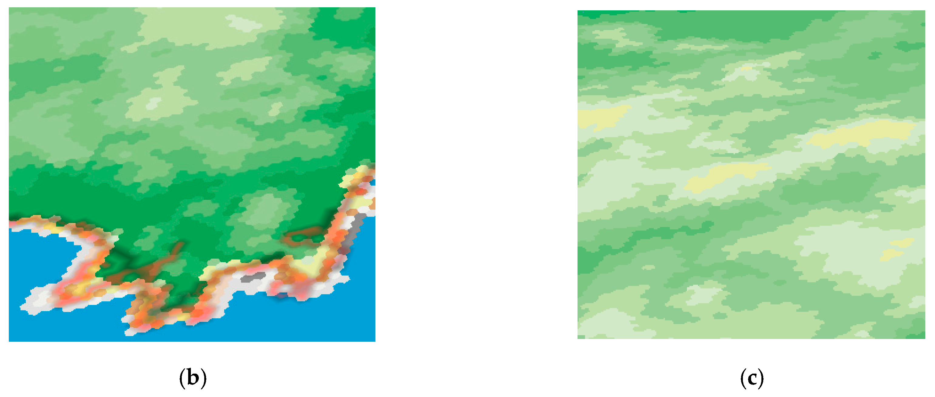
The resampling results are shown in Figure 13. To show the global terrain vividly, the hypsometric tending method is applied to render the grid cells into different elevation ranges. The specific ranges of elevation and the colors used for each range are from a new world terrain map published in 2014 [34]. Four different views of the globe are given in Figure 13 where Figure 13a,b,c, and d mainly show the areas of Europe and Asia, Antarctica, North America and South America, and Africa respectively. Figure 14 gives more details. In Figure 14a, we add the vector grid line of the boundary of China to verify the accuracy of the result. In Figure 14b,c, the rendered hexagonal cells can be seen clearly.
4.2. Discretization of the Spherical Vector Line Based on Hexagonal Grids and Index Arithmetics
A DGGS should also support vector data. Vector data are used to describe geospatial features—namely, points, lines, and polygons mainly—and are usually represented by coordinates of a series of points or a single point. In DGGS, vector data points should be approximated by grid cells, and the resolution of the grid cells is determined by the error of vector data or other specific need.
Current research indicates that the discretization of vector lines is the premise and basis of the discretization of vector data [35]. Most of study on the rasterization of line features is based on triangular or quadrilateral grids on the planes and fewer are based on hexagonal grids. In addition, discretization of vector lines on the sphere is far more complicated than on a plane because the spherical grids are usually irregular, and the relationship between the line and grid cells needs to be judged one by one, the process of which will involve spherical geometry operations and will impact the efficiency.
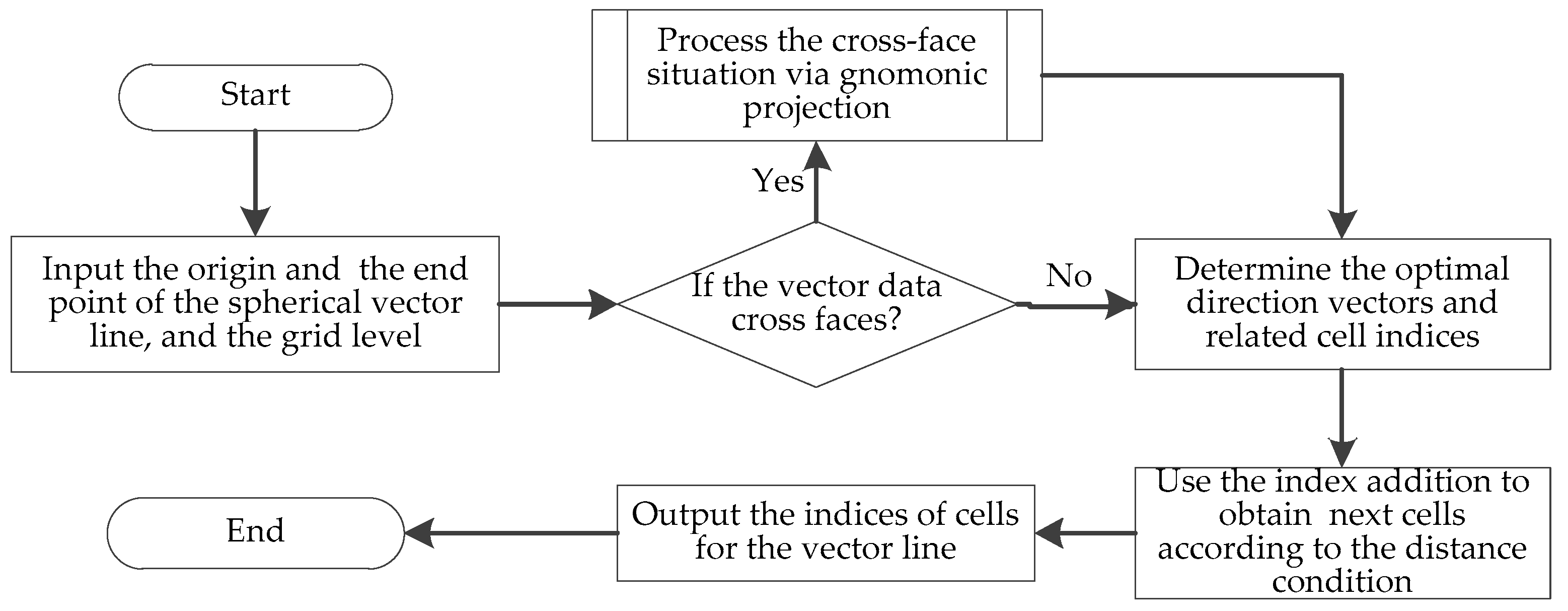
Our research group has proposed one algorithm to solve the above problems, called “duality and dimensionality reduction discrete line generation algorithm” [35]. In this algorithm, the index arithmetics of hexagonal grids is used to replace spherical geometry operation of coordinates of cells in generating the discrete vector line. Because discussing this algorithm needs long length and this part is not the emphasis of this paper, this experiment just directly uses the idea of this algorithm. The specific flowchart of this algorithm is shown in Figure 15.
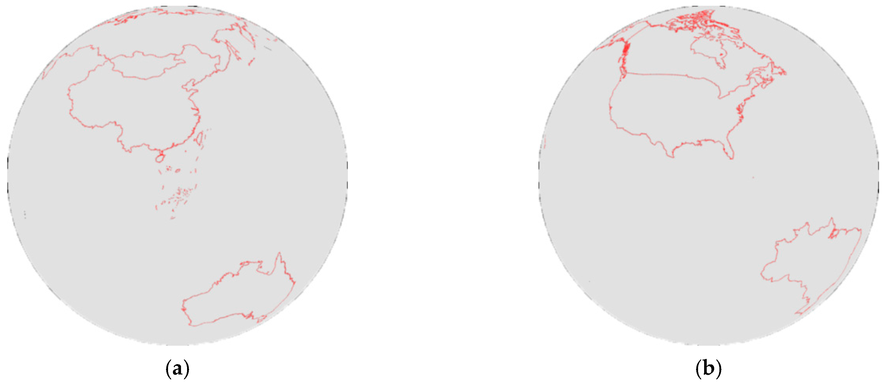
The above algorithm using our proposed index addition is compared with the algorithm using spherical geometry operations to realize the discretization of the vector lines on the sphere. The two algorithms are both implemented in C++ and compiled into the release version and executed on a compatible PC (Hardware configuration: Intel Core i5-6500 [email protected] GHz, 8 GB RAM and Kingston 120GB SSD; Operating System: Windows 7 X64 Ultimate SP1; Development Tools: Visual Studio 2012 Update 5). The vector data for this experiment are the boundaries of six countries—namely, China, America, Canada, Russia, Brazil, and Australia—and are obtained from the 1:250,000 basic geographic information database of the Chinese State Bureau of Surveying and Mapping. Each boundary is considered a closed polygon. The discretization result of our algorithm is shown in Figure 16. We also calculate statistics on the generation efficiency of discrete lines for the two algorithms from grid levels 16 to 20. The number of grid cells rasterized unit time, which is 1 ms in this paper, is used as the measurement of efficiency, thus the higher the values, the better the performance. The generation efficiency of the two algorithm is shown in Table 4 and Table 5. In the two tables, the left column represents the countries the tested vector boundary data belong to the following five columns are the related efficiency of different country boundaries from level 16 to level 20, and the last column is the average generation efficiency of the five levels.
The above comparison results indicate that the average generation efficiency of the algorithm using our proposed index arithmetics of the mixed aperture 3 and 4 icosahedral Snyder equal-area hexagonal DGGS is higher than that of the algorithm using traditional spherical geometry operations. The main reasons are as follows:
(1) From level 17 and higher levels, the efficiency of the algorithm based on the proposed method is higher than that based on spherical geometry calculation, as index addition can realize the rapid calculation of the topological relationship of hexagonal cells, which avoids calculations based on geometric distances, thereby improving the efficiency.
(2) Index addition realizes the three-dimensional location changes in the spherical space by searching the 1D integer addition tables stored before the operation. It essentially reduces the dimensions for problems with high dimensions, and therefore has higher efficiency.
(3) At level 16, the efficiency of the algorithm based on the proposed method is lower than that of another algorithm. It is because at the lower levels, the number of cells to generate is obviously smaller so that the advantage of replacing floating-point calculation with integer indexing arithmetic has not fully embodied because the number of integer calculations is relatively small, but the cells generated in the time of one frame can still meet the requirements of real-time 3D visualization. In addition, the resolution for level 16 in the mixed aperture hexagonal DGGS is about 1km and for level 20 and higher levels, the resolution can up to the scale of meters. Our algorithm can be efficient for finer resolution. With the data resolution finer, the geospatial application for fine resolution will be more. Our approach is obviously superior in higher levels and is more suitable to be used.
(4) The generation efficiency of our algorithm does not achieve a great improvement. When calculating the distance condition, the algorithm needs to use the inverse Snyder polyhedral projection to convert the cell indices into geographical coordinates, but the inverse Snyder projection requires iterative root finding approaches, which limits the improvement of our algorithm.
5. Conclusions and Future Work
Hexagonal DGGSs provide efficient solutions for digital earth. Most hexagonal DGGS now are pure aperture sequences that restrict the grid resolutions. This paper introduces how to index the mixed aperture 3 and 4 hexagonal DGGS. The proposed framework is based on an icosahedron. Combinations of two apertures can produce more resolutions in a finite resolution range. A general hierarchy-based method considering cell directions is designed first. Then, associated indexing arithmetics, including the operation rule and the implementation algorithm, is given. To extend the indexing method into the surface of the icosahedron, this paper designs an icosahedral grid structure formed by two types of grid tiles. Finally, the Snyder equal-area projection is used to construct the spherical grids.
This framework is more flexible than the existing pure aperture ones. It can determine the aperture sequence to obtain a grid resolution closest to the target resolution to save data volume. The whole scheme is applicable to all possible sequences and types of child cells of mixed aperture 3 and 4 schemes, and thus can provide more choices for DGGS users. The experiments provide idea about the possible applications where hexagonal DGGS and its indexing arithmetic can be efficient and useful, but more algorithms are required to develop for geospatial applications.
In the future work, aperture 7 will be further considered in our system on the basis of current research. In addition, the computational efficiency of our scheme is restricted by the iteration process of Snyder projection, which requires further improvement. Deeper research on applications of datasets should also be developed.
Author Contributions
Conceptualization, Rui Wang and Jin Ben; Methodology, Rui Wang; Software, Rui Wang and Jin Ben; Validation, Rui Wang and Jin Ben; Formal Analysis, Rui Wang; Investigation, Jianbin Zhou and Mingyang Zheng; Resources Jianbin Zhou; Data Curation, Mingyang Zheng; Writing—original draft preparation, Rui Wang and Jin Ben; Writing—review and editing, Rui Wang, Jin Ben, and Jianbin Zhou; Visualization, Rui Wang; Supervision, Jin Ben. All authors have read and agreed to the published version of the manuscript.
Funding
This research was funded by the National Key Research and Development Program of China, grant no. 2018YFB0505301, and the Natural Science Foundation of China, grant no. 41671410.
Conflicts of Interest
The authors declare no conflict of interest.
Appendix A
In this example, the mixed aperture 3 and 4 hexagonal grid is defined as: the grid has four levels from level 0 to level 3; the aperture sequence is 434; the initial cells for the level 0 are as Figure A1 shows. The digit sets for the chosen types of generated children cells of the three apertures are respectively {0,1,5,6} for the level 1, {0,B,C} for the level 2 and {0,A,C,E} for the level 3. The addition tables for the digit positions at the level 3 to the level 1 are seen in Table A1 where carry digit 0 is omitted until the first non-zero digit appears.
If we calculate two indices belonging to the level 3, such as , the specific process using addition tables are as follows:
- Calculate at the right digit position using Table A1c and get , where is the result index of the right digit position, and 5 and are respectively the carry digit for the digit position of the level 1 and the level 2.
- Calculate using Table A1b for the level 2 digit position, where is the result index of the digit position of the level 2, and 4 and 6 are respectively the carry digit for the digit position of the level 0 and the level 1.
- Calculate using Table A1a, and . There, 1 is the result index of the digit position of the level 1, and 2 and 6 are two carry digits for the level 0.
- Calculate at the left digit position and according to the definition in Figure A1.
Above all, .
Figure A1.
An example of the definition of the initial cells at the level 0: this example assigns 7 cells for the level 0 (source—own study).
Figure A1.
An example of the definition of the initial cells at the level 0: this example assigns 7 cells for the level 0 (source—own study).


Table A1.
An example of addition tables for the grid with 4 levels: (a) addition table for the digit position of the level 1; (b) addition table for the digit position of the level 2; (c) addition table for the digit position of the level 3.
Table A1.
An example of addition tables for the grid with 4 levels: (a) addition table for the digit position of the level 1; (b) addition table for the digit position of the level 2; (c) addition table for the digit position of the level 3.

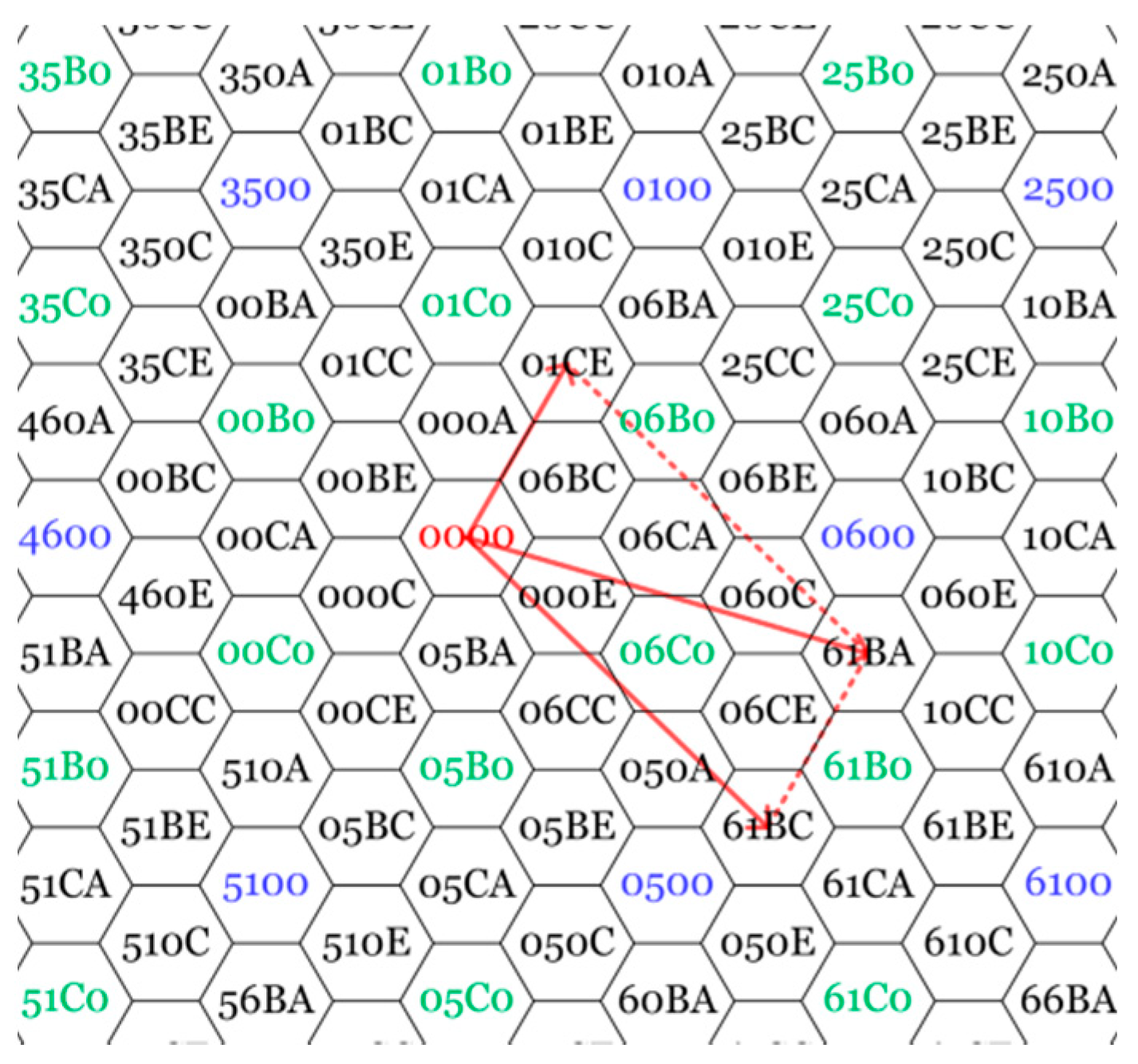
Part of the level 3 for the defined grid system is illustrated in Figure A2 and the addition of and is marked in red lines. The index addition meets parallelogram law on the plane because indexes are just the 1D representation of 2D vectors. The result is consistent with that calculated by addition tables above.
Figure A2.
Illustration of part of the defined grid system.

References
- Guo, H.D.; Liu, Z.; Jiang, H.; Wang, C.L.; Liu, J.; Liang, D. Big earth data: A new challenge and opportunity for Digital Earth’s development. Int. J. Digit. Earth 2017, 10, 1–12. [Google Scholar] [CrossRef] [Green Version]
- Mahdavi-Amiri, A.; Alderson, T.; Samavati, F. A survey of digital earth. Comput. Graph. 2015, 53, 95–117. [Google Scholar] [CrossRef]
- Sahr, K. On the optimal representation of vector location using fixed-width multi-precision quantizers. In Proceedings of the International Archives of the Photogrammetry, Remote Sensing and Spatial Information Science, Xuzhou, China, 11–12 November 2013. [Google Scholar] [CrossRef] [Green Version]
- Sahr, K.; White, D.; Kimerling, A.J. Geodesic discrete global grid systems. Cartogr. Geogr. Inf. Sci. 2003, 30, 121–134. [Google Scholar] [CrossRef] [Green Version]
- Adams, B. WÄhi, a discrete global grid gazetteer built using linked open data. Int. J. Digit. Earth 2017, 10, 490–503. [Google Scholar] [CrossRef]
- Lin, B.X.; Zhou, L.C.; Xu, D.P.; Zhu, A.X.; Lu, G.N. A discrete global grid system for earth system modelling. Int. J. Geogr. Inf. Sci. 2017, 4, 1–27. [Google Scholar]
- Yao, X.C.; Li, G.Q.; Xia, J.S.; Ben, J.; Cao, Q.; Zhao, L.; Ma, Y.; Zhang, L.; Zhu, D. Enabling the Big Earth Observation Data via Cloud Computing and DGGS: Opportunities and Challenges. Remote. Sens. 2019, 12, 62. [Google Scholar] [CrossRef] [Green Version]
- Topic 21: Discrete Global Grid Systems Abstract Specification. Available online: http://docs.opengeospatial.org/as/15-104r5/15-104r5.html (accessed on 13 November 2019).
- Sahr, K. Hexagonal discrete global grid systems for geospatial computing. Arch. Photogramm. Cartogr. Remote Sens. 2011, 22, 363–376. [Google Scholar]
- Vince, A.; Zheng, X.X. Arithmetic and fourier transform for the PYXIS multi-resolution digital earth model. Int. J. Digit. Earth 2009, 2, 59–79. [Google Scholar] [CrossRef]
- Why Hexagons? Available online: https://pro.arcgis.com/zh-cn/pro-app/tool-reference/spatial-statistics/h-whyhexagons.htm (accessed on 13 November 2019).
- Mahdavi-Amiri, A.; Bhojani, F.; Samavati, F. One-to-two digital earth. In Proceedings of the 9th International Symposium on Advances in Visual Computing (ISVC 2013), Rethymnon, Greece, 29–31 July 2013; Springer: Berlin/Heidelberg, Germany, 2013. [Google Scholar] [CrossRef]
- Sahr, K. Central place indexing: Hierarchical linear indexing systems for mixed-aperture hexagonal discrete global grid systems. Cartographica 2019, 54, 16–29. [Google Scholar] [CrossRef]
- Mahdavi Amiri, A.; Alderson, T.; Samavati, F. Geospatial data organization methods with emphasis on aperture-3 hexagonal discrete global grid systems. Cartographica 2019, 54, 30–50. [Google Scholar] [CrossRef]
- Sahr, K. Location coding on icosahedral aperture 3 hexagon discrete global grids. Comput. Environ. Urban Syst. 2008, 32, 174–187. [Google Scholar] [CrossRef]
- Tong, X.C.; Ben, J.; Wang, Y.; Zhang, Y.S.; Pei, T. Efficient encoding and spatial operation scheme for aperture 4 hexagonal discrete global grid system. Int. J. Geogr. Inf. Sci. 2013, 27, 898–921. [Google Scholar] [CrossRef]
- Wang, R.; Ben, J.; Du, L.Y.; Zhou, J.B.; Li, Z.X. Encoding and operation for the planar aperture 4 hexagon grid system. Acta Geotech. Cartogr. Sin. 2018, 47, 1018–1025. [Google Scholar] [CrossRef]
- Cozzi, P.; Ring, K. 3D Engine Design for Virtual Globes, 1st ed.; A K Peters, Ltd.: Natick, MA, USA, 2011. [Google Scholar]
- Tobler, W.; Chen, Z.T. A quadtree for global information storage. Geogr. Anal. 1986, 18, 360–371. [Google Scholar] [CrossRef]
- Gibb, R.G. The rHEALPix discrete global grid system. In Proceedings of the IOP Conference Series: Earth and Environmental Science, Halifax, NS, Canada, 16 May 2016; Volume 34, p. 012012. [Google Scholar] [CrossRef] [Green Version]
- Ben, J.; Tong, X.C.; Zhou, C.H.; Zhang, K.X. Construction algorithm of octahedron based hexagon grid systems. J. Geo-Inf. Sci. 2015, 6, 54–61. [Google Scholar] [CrossRef]
- Bai, J.J. Location coding and indexing aperture 4 hexagonal discrete global grid based on octahedron. J. Remote Sens. 2011, 15, 1125–1137. [Google Scholar]
- White, D.; Kimerling, A.J.; Sahr, K.; Lian, S. Comparing area and shape distortion on polyhedral-based recursive partitions of the sphere. Int. J. Geogr. Inf. Sci. 1998, 12, 805–827. [Google Scholar] [CrossRef]
- Mahdavi-Amiri, A.; Harrison, E.; Samavati, F. Hexagonal connectivity maps for Digital Earth. Int. J. Digit. Earth 2014, 8, 750–769. [Google Scholar] [CrossRef]
- Wang, R.; Ben, J.; Du, L.Y.; Zhou, J.B.; Li, Z.X. The code operation scheme for the icosahedral aperture 4 hexagon grid system. Geomat. Inf. Sci. Wuhan Univ. 2019. [Google Scholar] [CrossRef]
- H3. Available online: https://uber.github.io/h3/#/ (accessed on 13 November 2019).
- Vince, A. Indexing the aperture 3 hexagonal discrete global grid. J. Vis. Commun. Image Represent. 2006, 17, 1227–1236. [Google Scholar] [CrossRef]
- PYXIS. Available online: http://pyxisinnovation.com (accessed on 13 November 2019).
- Ben, J.; Li, Y.L.; Zhou, C.H.; Wang, R.; Du, L.Y. Algebraic encoding scheme for aperture 3 hexagonal discrete global grid system. Sci. China-Earth Sci. 2018, 61, 215–227. [Google Scholar] [CrossRef]
- Gibson, L.; Lucas, D. Spatial data processing using generalized balanced ternary. In Proceedings of the IEEE Computer Society Conference on Pattern Recognition and Image Processing, Las Vegas, NV, USA; 1982; pp. 566–571. [Google Scholar]
- Sahr, K. Central Place Indexing Systems. United States Patent Awarded U.S. 2,010,054,550, 6 August 2012. [Google Scholar]
- Snyder, J. An equal-area map projection for polyhedral globes. Cartographica 1992, 29, 10–21. [Google Scholar] [CrossRef]
- USGS EROS Archive-Digital Elevation-Global 30 Arc-Second Elevation (GTOPO30). Available online: https://www.usgs.gov/centers/eros/science/usgs-eros-archive-digital-elevation-global-30-arc-second-elevation-gtopo30?qt-science_center_objects=0#qt-science_center_objects (accessed on 13 November 2019).
- She, S.J.; Liao, X.Y.; Xue, H.P.; Xu, H.Q.; Zhang, H.M.; Xu, Z.J.; Deng, J.F. Special representation of the Antaritic ice sheet on the world terrain map. Geospat. Inf. 2014, 12, 142–143. [Google Scholar] [CrossRef]
- Du, L.Y.; Ma, Q.H.; Ben, J.; Wang, R.; Li, J.H. Duality and dimensionality reducation discrete line generation algorithm for a triangular grid. ISPRS Int. J. Geo-Inf. 2018, 7, 391. [Google Scholar] [CrossRef] [Green Version]
Figure 1.
Five base polyhedrons for Discrete Global Grid Systems (DGGSs): (a) tetrahedron; (b) cube; (c) octahedron; (d) dodecahedron; (e) icosahedron (Source—cited from [8]).
Figure 1.
Five base polyhedrons for Discrete Global Grid Systems (DGGSs): (a) tetrahedron; (b) cube; (c) octahedron; (d) dodecahedron; (e) icosahedron (Source—cited from [8]).

Figure 2.
The general idea of using the icosahedron to construct the hexagonal DGGS: (a) the planar hexagonal grid system; (b) the icosahedral hexagonal grid system; (c) the hexagonal DGGS obtained by projecting the (b) (source—own study).
Figure 2.
The general idea of using the icosahedron to construct the hexagonal DGGS: (a) the planar hexagonal grid system; (b) the icosahedral hexagonal grid system; (c) the hexagonal DGGS obtained by projecting the (b) (source—own study).

Figure 3.
The neighboring relationship for different cell types: (a) triangles; (b) quads; (c) hexagons. d1 and d2 are distances between two neighboring cells (source—own study).
Figure 3.
The neighboring relationship for different cell types: (a) triangles; (b) quads; (c) hexagons. d1 and d2 are distances between two neighboring cells (source—own study).

Figure 4.
Centroid alignment and vertex alignment of three apertures for hexagonal grids (shown in orange and red, respectively): (a) and (b) are for aperture 3; (c) and (d) are for aperture 4; (e) and (f) are for aperture 7 (source—cited from [24]).
Figure 4.
Centroid alignment and vertex alignment of three apertures for hexagonal grids (shown in orange and red, respectively): (a) and (b) are for aperture 3; (c) and (d) are for aperture 4; (e) and (f) are for aperture 7 (source—cited from [24]).

Figure 5.
Diagram of mixed aperture 3 and 4: (a) aperture sequence 34; (b) aperture sequence 43. The red cells are the initial cells at level 0; the black cells belong to level 1; the orange cells belong to level 2 (source—own study).
Figure 5.
Diagram of mixed aperture 3 and 4: (a) aperture sequence 34; (b) aperture sequence 43. The red cells are the initial cells at level 0; the black cells belong to level 1; the orange cells belong to level 2 (source—own study).

Figure 6.
Types of child cells generated to ensure the uniqueness of indexing: (a) and (b) are for aperture 3; (c) and (d) are for aperture 4. The gray cells are the chosen child cells of the parent cell (source—partly refer to [13]).
Figure 6.
Types of child cells generated to ensure the uniqueness of indexing: (a) and (b) are for aperture 3; (c) and (d) are for aperture 4. The gray cells are the chosen child cells of the parent cell (source—partly refer to [13]).

Figure 7.
Two types of cell directions for the mixed aperture 3 and 4 hexagonal grids on the plane and the digits are marked for each basic vector of cell direction: (a) the first type of cell direction; (b) the second type of cell direction (source—own study).
Figure 7.
Two types of cell directions for the mixed aperture 3 and 4 hexagonal grids on the plane and the digits are marked for each basic vector of cell direction: (a) the first type of cell direction; (b) the second type of cell direction (source—own study).

Figure 8.
Diagram of the proposed hierarchy-based indexing method with aperture sequence 43 from level n to level n+2. The type of child cells for aperture 4 is from Figure 6c, and that for aperture 3 is from Figure 6b (source—own study).

Figure 9.
The IJK coordinate system defined for mixed aperture 3 and 4 hexagonal grids: (a) is used in the first type of cell directions and (b) is used in the second type (source—own study).
Figure 9.
The IJK coordinate system defined for mixed aperture 3 and 4 hexagonal grids: (a) is used in the first type of cell directions and (b) is used in the second type (source—own study).

Figure 10.
Two types of tiles on the unfolded faces of the icosahedron including 20 face tiles (gray) and 12 vertex tiles (white). The indices of each face and vertex are marked (source—own study).
Figure 10.
Two types of tiles on the unfolded faces of the icosahedron including 20 face tiles (gray) and 12 vertex tiles (white). The indices of each face and vertex are marked (source—own study).

Figure 11.
Diagram of conversion between indices and geographical coordinates (source—own study).

Figure 12.
Illustration of the data redundancy of GTOPO30: The sampling diagram of GTOPO30 in which the arc intervals of latitude and longitude for cells are uniform (source—cited from online).
Figure 12.
Illustration of the data redundancy of GTOPO30: The sampling diagram of GTOPO30 in which the arc intervals of latitude and longitude for cells are uniform (source—cited from online).

Figure 13.
Resampling results of the GTOPO30 DEM dataset based on the proposed scheme: The four figures are different views of the globe: (a) Europe and Asia; (b) Antarctica; (c) North America and South America; (d) Africa (source—own study).
Figure 13.
Resampling results of the GTOPO30 DEM dataset based on the proposed scheme: The four figures are different views of the globe: (a) Europe and Asia; (b) Antarctica; (c) North America and South America; (d) Africa (source—own study).

Figure 14.
Details of the resampling results of GTOPO30 dataset based on the mixed aperture 3 and 4 scheme: (a) involves the area of China; (b) and (c) are more detailed figures to show the hexagonal cells more clearly (source—own study).
Figure 14.
Details of the resampling results of GTOPO30 dataset based on the mixed aperture 3 and 4 scheme: (a) involves the area of China; (b) and (c) are more detailed figures to show the hexagonal cells more clearly (source—own study).


Figure 15.
Flowchart of discretizing the vector line on the sphere using hexagonal grids: the process in this algorithm (except the index addition) is referred to the literature [35] (source—partly cited from [35] and changed according to own study).

Figure 16.
Results of the vector lines using hexagonal grids: the vector lines are the boundries of different countries. (a) contains China, Russia and Australia and (b) contains America, Canada and Brazil.
Figure 16.
Results of the vector lines using hexagonal grids: the vector lines are the boundries of different countries. (a) contains China, Russia and Australia and (b) contains America, Canada and Brazil.

Table 1.
Addition tables for the proposed indexing method: (a) for digits of aperture 3; (b) for digits of aperture 4
Table 1.
Addition tables for the proposed indexing method: (a) for digits of aperture 3; (b) for digits of aperture 4

Table 2.
Chosen grid level for different icosahedral hexagonal Discrete Global Grid System (DGGS) schemes. The projection for all schemes is Snyder equal-area polyhedral projection.
Table 2.
Chosen grid level for different icosahedral hexagonal Discrete Global Grid System (DGGS) schemes. The projection for all schemes is Snyder equal-area polyhedral projection.
| DGGS Scheme | Chosen Grid Level | Aperture Sequence | Number of Cells | Cell Area (km2) | |
|---|---|---|---|---|---|
| Aperture 3 | 17 | 1,291,401,632 | 0.39497 | ||
| Aperture 4 | 13 | 671,088,642 | 0.76006 | ||
| Aperture 7 (H3) | 8 | 691,776,122 | 0.73733 | ||
| Mixed aperture 3 and 4 | 16 | 1 aperture 4 | 573,956,282 | 0.88868 | |
Table 3.
Comparison of data volume for different schemes
| Scheme | Number of Cells | Percent of Data Volume (%) |
|---|---|---|
| GTOPO30 | 933,120,000 | 38.5 |
| The proposed scheme | 573,956,282 |
Table 4.
Discretization efficiency (number of cells rasterized ms−1) of the spherical vector lines using the proposed index arithmetic.
Table 4.
Discretization efficiency (number of cells rasterized ms−1) of the spherical vector lines using the proposed index arithmetic.
| 16 | 17 | 18 | 19 | 20 | Average Efficiency | ||
|---|---|---|---|---|---|---|---|
| China | 204.70 | 202.10 | 199.38 | 202.07 | 200.39 | 201.73 | |
| Australia | 198.34 | 200.90 | 204.18 | 195.65 | 203.59 | 200.53 | |
| Russia | 192.50 | 197.63 | 198.41 | 201.68 | 203.83 | 198.81 | |
| America | 199.26 | 202.11 | 201.02 | 203.85 | 203.10 | 201.87 | |
| Canada | 193.50 | 200.33 | 203.17 | 203.62 | 197.53 | 199.63 | |
| Brazil | 188.57 | 197.62 | 200.46 | 200.86 | 201.86 | 197.87 | |
Table 5.
Discretization efficiency (number of cells rasterized ms−1) of the spherical vector lines using traditional spherical geometry operation.
Table 5.
Discretization efficiency (number of cells rasterized ms−1) of the spherical vector lines using traditional spherical geometry operation.
| Level | 16 | 17 | 18 | 19 | 20 | Average Efficiency | |
|---|---|---|---|---|---|---|---|
| Country | |||||||
| China | 255.80 | 207.18 | 178.98 | 85.25 | 102.94 | 166.03 | |
| Australia | 248.71 | 201.29 | 186.78 | 161.86 | 119.99 | 183.73 | |
| Russia | 226.57 | 188.33 | 164.26 | 132.02 | 100.29 | 162.29 | |
| America | 220.37 | 188.53 | 149.44 | 113.59 | 70.00 | 148.39 | |
| Canada | 203.40 | 173.81 | 186.54 | 152.20 | 109.01 | 164.99 | |
| Brazil | 243.04 | 220.14 | 188.92 | 157.71 | 114.91 | 184.94 | |
© 2020 by the authors. Licensee MDPI, Basel, Switzerland. This article is an open access article distributed under the terms and conditions of the Creative Commons Attribution (CC BY) license (http://creativecommons.org/licenses/by/4.0/).
Share and Cite
MDPI and ACS Style
Wang, R.; Ben, J.; Zhou, J.; Zheng, M. Indexing Mixed Aperture Icosahedral Hexagonal Discrete Global Grid Systems. ISPRS Int. J. Geo-Inf. 2020, 9, 171. https://0-doi-org.brum.beds.ac.uk/10.3390/ijgi9030171
AMA Style
Wang R, Ben J, Zhou J, Zheng M. Indexing Mixed Aperture Icosahedral Hexagonal Discrete Global Grid Systems. ISPRS International Journal of Geo-Information. 2020; 9(3):171. https://0-doi-org.brum.beds.ac.uk/10.3390/ijgi9030171
Chicago/Turabian StyleWang, Rui, Jin Ben, Jianbin Zhou, and Mingyang Zheng. 2020. "Indexing Mixed Aperture Icosahedral Hexagonal Discrete Global Grid Systems" ISPRS International Journal of Geo-Information 9, no. 3: 171. https://0-doi-org.brum.beds.ac.uk/10.3390/ijgi9030171
Note that from the first issue of 2016, this journal uses article numbers instead of page numbers. See further details here.