DM-SLAM: A Feature-Based SLAM System for Rigid Dynamic Scenes


1
School of Remote Sensing and Information Engineering, Wuhan University, Wuhan 430070, China
2
Shenzhen Jimuyida Technology Co., Ltd., Shenzhen 518000, China
3
School of Software Engineering, Xi’an Jiaotong University, Xi’an 710049, China
4
School of Resource and Environment Sciences, Wuhan University, Wuhan 430070, China
*
Author to whom correspondence should be addressed.
ISPRS Int. J. Geo-Inf. 2020, 9(4), 202; https://0-doi-org.brum.beds.ac.uk/10.3390/ijgi9040202
Submission received: 25 February 2020
/
Revised: 18 March 2020
/
Accepted: 23 March 2020
/
Published: 27 March 2020
(This article belongs to the Special Issue 3D Indoor Mapping and Modelling)
Abstract
:Most Simultaneous Localization and Mapping (SLAM) methods assume that environments are static. Such a strong assumption limits the application of most visual SLAM systems. The dynamic objects will cause many wrong data associations during the SLAM process. To address this problem, a novel visual SLAM method that follows the pipeline of feature-based methods called DM-SLAM is proposed in this paper. DM-SLAM combines an instance segmentation network with optical flow information to improve the location accuracy in dynamic environments, which supports monocular, stereo, and RGB-D sensors. It consists of four modules: semantic segmentation, ego-motion estimation, dynamic point detection and a feature-based SLAM framework. The semantic segmentation module obtains pixel-wise segmentation results of potentially dynamic objects, and the ego-motion estimation module calculates the initial pose. In the third module, two different strategies are presented to detect dynamic feature points for RGB-D/stereo and monocular cases. In the first case, the feature points with depth information are reprojected to the current frame. The reprojection offset vectors are used to distinguish the dynamic points. In the other case, we utilize the epipolar constraint to accomplish this task. Furthermore, the static feature points left are fed into the fourth module. The experimental results on the public TUM and KITTI datasets demonstrate that DM-SLAM outperforms the standard visual SLAM baselines in terms of accuracy in highly dynamic environments.
1. Introduction
Simultaneous Localization and Mapping (SLAM) is one of the key technologies in the field of intelligent mobile robots. Over the past few decades, many state-of-the-art algorithms have been proposed and achieved satisfactory performance in most static scenes. SLAM techniques utilize the data streams of on-board sensors to dynamically build a map model for the current environment in an incremental way and estimate the position during the map construction process. Visual SLAM is the SLAM system with a camera as the main sensor, which has received extensive attention and been widely researched in recent years. Compared with other sensors, such as LiDAR, visual SLAM is much less costly and can obtain a larger amount of data about surrounding environments. Many visual SLAM systems have achieved excellent performance under certain circumstances (e.g., DTAM [1], LSD-SLAM [2], and ORB-SLAM2 [3]). However, it is challenging for almost all existing visual SLAM systems to provide accurate and robust location information in real-world environments because the ubiquitous moving objects will cause errors in the camera motion computation. There are several solutions for this problem, one of which is the traditional robust estimation methods such as RANSAC [4]. This method removes the dynamic information that occupies a small part of the scene as an outlier, but it may fail when dynamic objects dominate the scene. Another popular solution is to integrate information from additional sensors mounted on the robots [5]. The system can extract the dynamic objects from the scenes via ego-motion compensation using the information captured from several sensors. However, this is not a cost-effective method, and cameras are often the only sensors available. Therefore, in this paper, we focus on how to eliminate the effect of dynamic objects using only cameras.
Visual SLAM can be divided into two categories: feature-based methods [3,6,7] and direct methods [1,2,8,9]. Feature-based methods search for correspondences by comparing the descriptors of each feature point between images and optimize the camera pose by minimizing the reprojection error. Direct methods calculate the minimum photometric error to estimate the pose based on the grayscale invariant assumption. As analyzed by Engel et al. [10], these two methods have their advantages and disadvantages. Specifically, feature-based methods are significantly more robust to geometric noise, but the feature point extraction is time consuming. Direct methods perform better in low-texture regions than feature-based methods but are generally more sensitive to dynamic objects. However, none of the above methods can solve the problems caused by common dynamic objects in the scenes. The dynamic objects will produce many wrong data associations during the process, which can degrade the calculated pose accuracy.
When there are rigid or non-rigid objects with absolute motion in the rigid scene (e.g., people walking, moving cars, etc.), it is a rigid dynamic scene. In this paper, a novel visual SLAM method for rigid dynamic scenes (DM-SLAM) is proposed based on the ORB-SLAM2 system [3]. It applies an instance segmentation network and optical flow to eliminate the influence of the dynamic objects existing in the scenes. For cameras that can obtain depth information (RGB-D/stereo cameras) and monocular cameras, we present two strategies to detect dynamic points. In the RGB-D/stereo case, the feature points with depth information of the previous frame are reprojected to the current frame. Then, we use the reprojection offset vectors [u,v] to obtain an adaptive threshold to distinguish dynamic points. In the monocular case, our method calculates the distance from the matched point to its corresponding epipolar line. Those points whose distance exceeds the preset value are considered to be dynamic. The contributions of our work can be summarized as follows:
- We propose a complete visual SLAM system called DM-SLAM that combines an instance segmentation network and optical flow information. The system eliminates the influence of dynamic objects on pose estimation in highly dynamic environments and can handle data streams from monocular, stereo, and RGB-D sensors.
- We present two strategies to efficiently extract dynamic points between adjacent frames for RGB-D/stereo camera and monocular camera cases.
- We evaluate our proposed system on the public TUM and KITTI datasets and achieve good performance in highly dynamic scenarios. The absolute trajectory accuracy of DM-SLAM far outperforms those of the standard visual SLAM baselines.
2. Related Work
Dynamic objects are classified as outliers in most visual SLAM systems, which are not used for tracking and mapping. In addition to the SLAM systems using typical outlier rejection algorithms [4], the methods of connecting deep learning with visual SLAM have also been extensively studied in recent years. Therefore, we will introduce the dynamic SLAM systems based on the traditional methods in Section 2.1 and the SLAM systems combined with deep learning in Section 2.2.
2.1. Dynamic SLAM
Different methods have been proposed to handle dynamic problems in visual SLAM in the past. Saputra et al. [11] discuss in detail visual SLAM and 3D reconstruction techniques in dynamic environments. The studies [12,13,14] use depth information and Alcantarilla et al. [15] use the scene flow to detect and eliminate the moving objects from the background. Tan et al. [16] project the map features from the closest keyframes to the current frame to detect changed points and propose an alternative RANSAC formulation to distribute the sampled points. However, when dynamic objects move slowly, this method has difficulty maintaining a robust motion estimation. Sun et al. [12] roughly filter out moving-object motions via ego-motion compensation and then precisely determine the foreground based on vector quantization. Wang et al. [14] cluster the RGB image-based trajectories of points; then, dynamic points are excluded via energy function minimization. Dense SLAM systems perform better after integrating this method. Optical flow is used to construct an angle histogram in [17]. They use the Gaussian Mixture Model (GMM) to approximate the obtained angle histogram and then estimate the parameters using the expectation–maximization (EM) algorithm. Finally, the Gaussians with sufficiently high mixing proportion are selected as optical flow over moving objects. Sabzevari et al. [18] employed the wheeled vehicle constraint to estimate the camera motion by utilizing Ackermann steering geometry. The feature points satisfying the motion estimation of the camera are static features and the others are considered as dynamic features. Maxime et al. [19] propose real-time monocular visual odometry for dynamic underwater environments. They utilize RANSAC to compute the essential matrix and eliminate the outliers that are not consistent with the epipolar geometry. However, the system lacks a loop-closure mechanism and cannot be regarded as a complete visual SLAM method. Liu et al. [20] combine the Grid-based Motion Statistics (GMS) GMS [21] feature matching algorithm and a sliding window to eliminate the influence of dynamic objects. Other approaches utilize external sensors such as an inertial measurement unit (IMU) to solve this problem [22,23] by estimating the camera ego-motion. Kim et al. [24] combine RGB-D sensors with an IMU to estimate camera pose in a highly dynamic environment. The IMU information is considered as a priori information to constrain the camera pose estimation and eliminate visual information error. In addition to these methods for dealing with rigid scenarios, Agudo et al. [25,26] provide a solution to handle a non-rigid objects based Kalman filter. The Navier–Cauchy equations are used to represent the object’s surface mechanics and are solved with a Finite Element Method (FEM). Then, they embed equations in an extended Kalman filter, resulting in a sequential Bayesian optimization framework.
2.2. SLAM Combined with Deep Learning
There have been some attempts to combine deep learning with visual SLAM to improve the performance of traditional SLAM systems. CNN-SLAM [27] is one of the typical approaches, which fuses CNN-predicted depth values with depth measurements directly calculated from monocular SLAM. DeTone et al. [28] propose a point tracking system using two deep convolution neural networks called MagicPoint and MagicWarp. The first network extracts 2D feature points, and the second processes pairs of point images. In addition, semantic segmentation networks are often applied in visual SLAM systems. Bowman et al. [29] use EM estimation to convert semantic SLAM into a probability problem. They utilize the traditional DPM detection network and still achieve certain effects. Lianos et al. [30] regard semantic information as constant scene rendering elements while using semantic reprojection errors to construct constraint conditions. Riazuelo et al. [31] embed a human tracker into the SLAM system and deal with the impact of walking people by using human semantic information. In [32], a semantic fusion approach is proposed to handle dynamic objects more efficiently. Kaneko et al. [33] present a framework for eliminating unstable feature points utilizing masks that are generated by a semantic segmentation network. The remaining feature points are used to stably estimate the camera position. Chao et al. [34] used the SegNet [35] network to obtain a pixel-wise semantic segmentation of the image and combine it with a motion consistency check to filter out dynamic portions of the scene. They produce a dense semantic octo-tree map, which can be used for high-level tasks but has less positioning accuracy in tracking. Similarly, Bescos et al. [36] propose DynaSLAM, which combines a multiview geometry and Mask R-CNN [37] to detect dynamic objects in the RGB-D case. However, in monocular and stereo cases, they simply do not extract feature points in the mask area, which means that the mask area is considered to be absolutely dynamic. This may result in tracking loss or initialization failure due to a small number of remaining feature points. Masoud et al. [38] propose an algorithm that integrates the feature-based SLAM with multi-target tracking (MTT) for dynamic environments. They use Faster R-CNN [39] to detect objects and classify them as moving and stationary objects. This algorithm only detects two categories of doors and people and cannot cope well with complex dynamic scenes.
3. System Introduction
In this section, the problem statement is first introduced. Then, we describe the details of our proposed method in Section 3.2.
3.1. Problem Statement
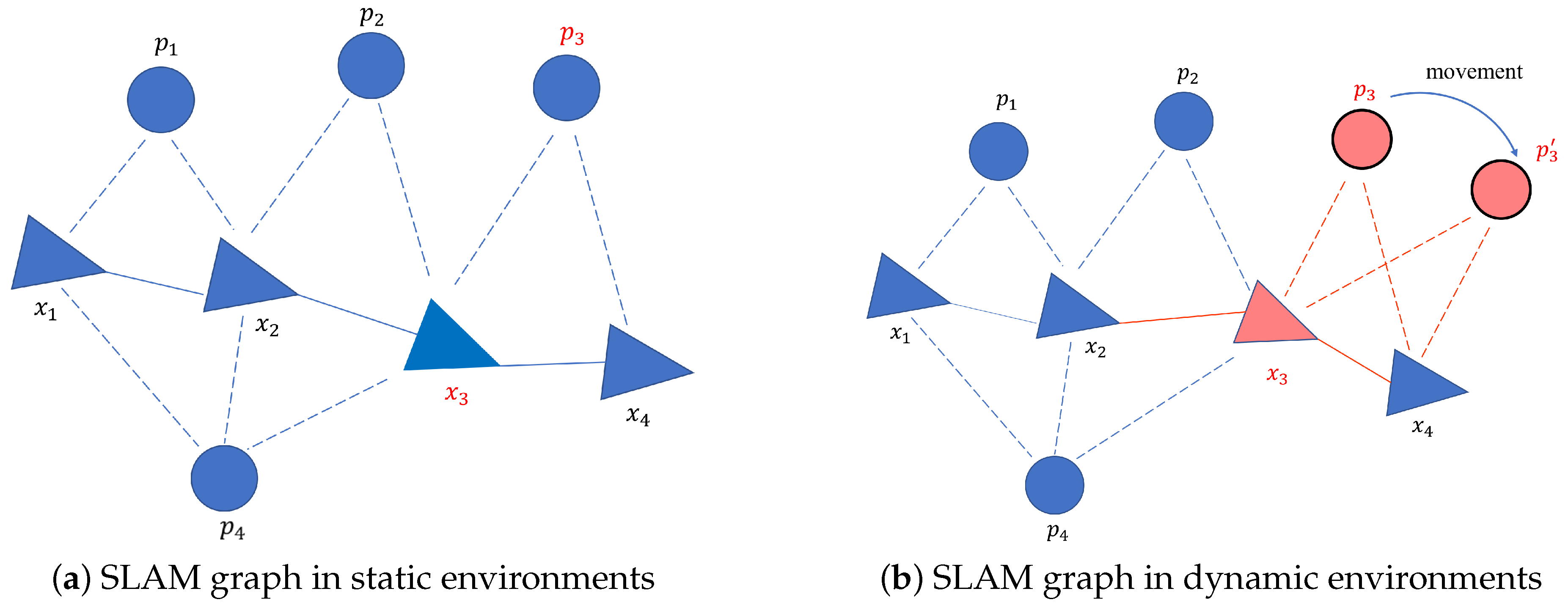
The graph optimization model in dynamic environments is shown in Figure 1. The motion model can be represented as the edges linking camera poses. The measurement model is represented as the edges linking camera poses and observed landmarks. The measurement model can be formulated as:
where denotes the Lie algebra representation of the camera pose at time k, and represents the position of the j-th landmark. The measurement is pixel coordinate information in the image taken by the camera, which corresponds to the observation of landmark j by the camera at time k. is the nonlinear model, and is Gaussian noise with zero mean assumed. denotes the covariance of the measurement. For this observation, the error term can be defined as:
Then, we can describe the cost function as follows:
where x denotes all camera poses and positions of landmarks. This is a typical nonlinear least square problem. However, if there are dynamic objects in the scene, they will corrupt the measurement model. As mentioned above, is assumed to have zero mean in Equation (1). Obviously, this term does not have a non-zero mean for the measurement of dynamic objects. The abnormal noise of non-zero mean will bring false information into the optimization process. As shown in Figure 1b, dynamic landmarks destroy the constraints of camera poses (red solid edges) and the constraints between camera poses and landmarks (red dotted edges).
Let denote the 2D location change of landmark j at time k. We can modify Equation (2) as follows:
where if the landmark j is static at time k, then is set to 0; otherwise, it is set to 1:
The cost function Equation (3) will also be fine-tuned accordingly. We can see that the tuning function aims to estimate the camera poses and landmark positions accurately by eliminating the negative effects of dynamic landmarks on this problem. The method of distinguishing dynamic objects will be described in Section 3.2.
3.2. Proposed Method
This section describes the proposed DM-SLAM method. DM-SLAM consists of four modules: semantic segmentation, ego-motion estimation, dynamic point detection, and a feature-based SLAM framework. In the following sections, the framework of DM-SLAM, segmentation of potentially moving objects, ego-motion estimation, and dynamic feature extraction are presented in detail.
3.2.1. Overview of the Proposed Approach
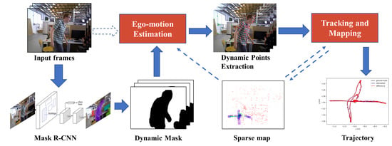
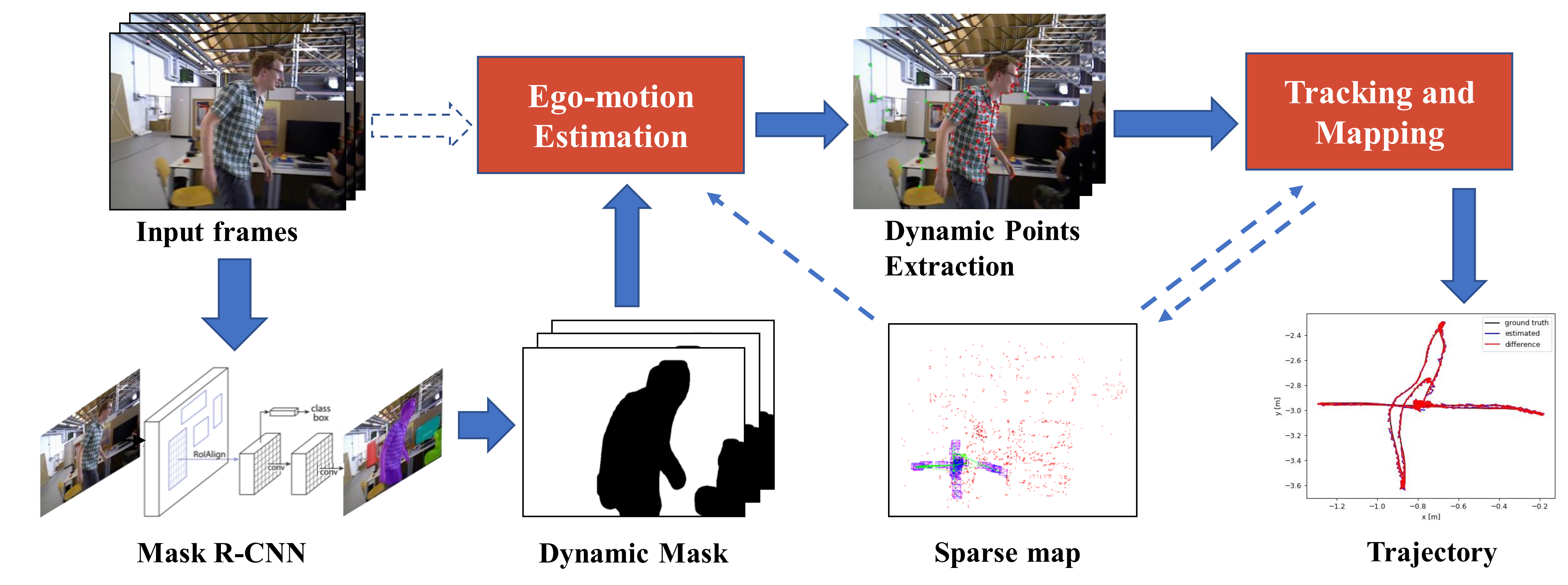
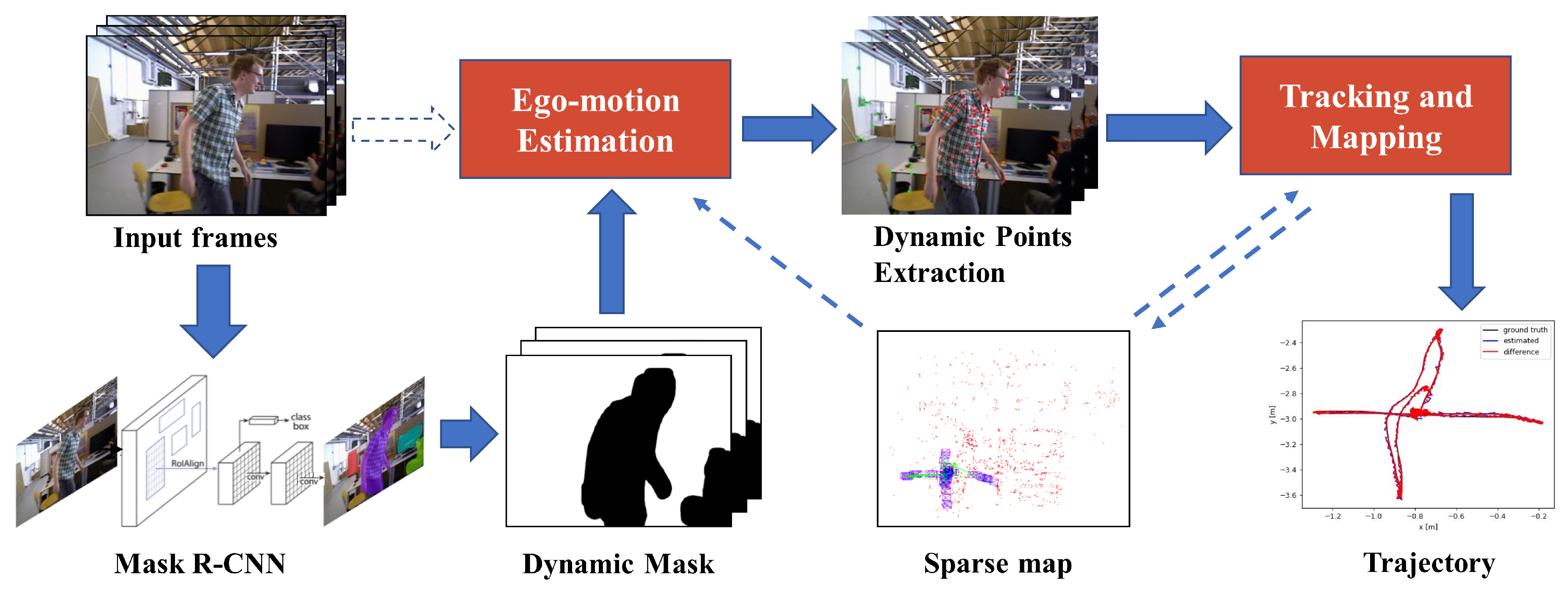
Figure 2 shows an overview of our proposed method, and Figure 3 shows in more detail the pipeline in monocular and RGB-D/stereo cases. The input frames are first segmented by Mask R-CNN. Then, we preliminarily assume that some of the segmented content are dynamic (e.g., people and cars). All the feature points that fall in the selected regions are discarded for rough ego-motion estimation. We adopt the low-cost tracking algorithm proposed in [36] to calculate the initial pose. Because there are fewer feature points involved in the pose estimation and lack of local bundle adjustment, the calculated initial pose is inaccurate.
As illustrated in Figure 3, we propose two different strategies to detect dynamic feature points after ego-motion estimation. In the monocular case (dotted line), we simply use the epipolar constraint to extract dynamic points. The distance from the matched points to its corresponding epipolar line is used to distinguish the outliers. In RGB-D/stereo cases (solid line), the feature points have depth information from the depth image or triangulation. We reproject the feature points of the previous frame to the current frame, and the reprojection offset vectors [u,v] are used to describe the offset distribution of the static area. Then, the feature points that do not follow the a priori distribution will be considered as dynamic points.
Subsequently, we utilize the dynamic feature points to determine whether the mask areas are dynamic. All of the feature points located in the corresponding dynamic content are discarded. The static feature points left are fed into the SLAM algorithm for tracking and mapping.
3.2.2. Segmentation of Potentially Moving Objects
To accurately detect the regions of dynamic objects, we adopt the Mask R-CNN [37] network to obtain both instance label and pixel-wise semantic segmentation based on TensorFlow.
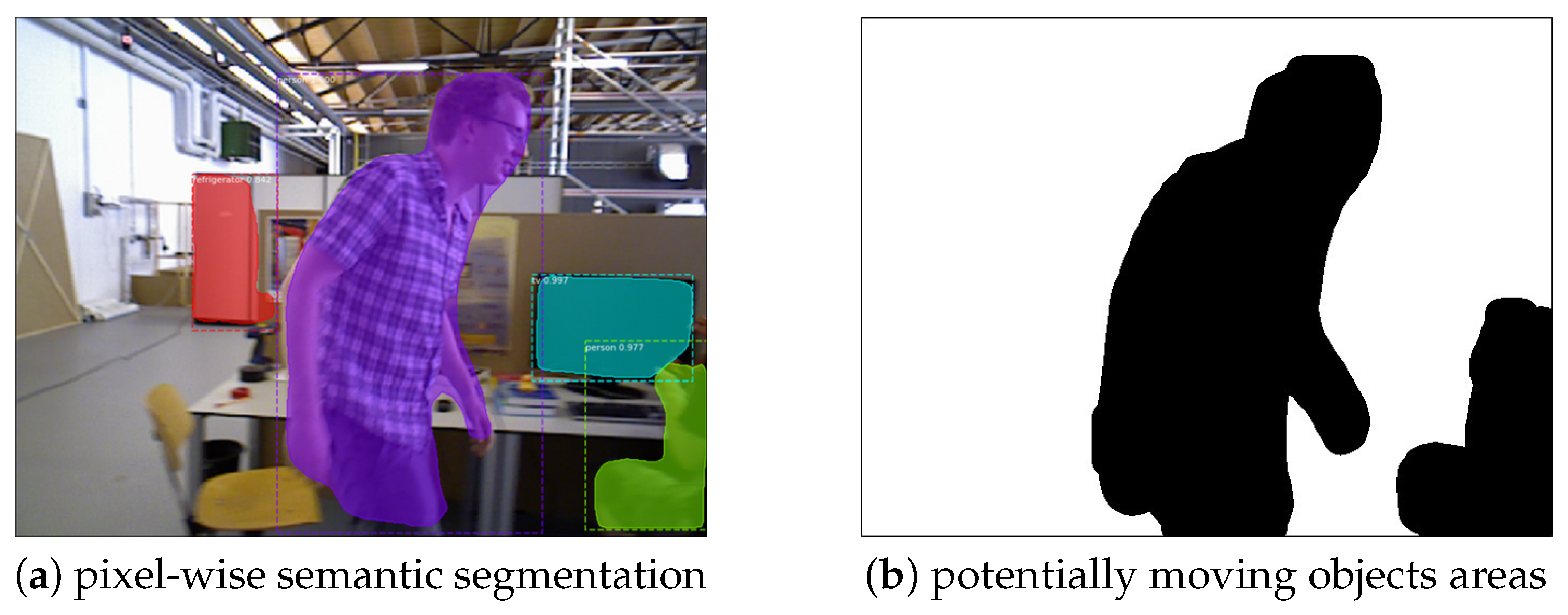
Mask R-CNN is one of the state-of-the-art instance segmentation networks, which can segment 80 classes trained on COCO datasets [40]. We employ the pre-trained models on COCO and select 20 of these 80 classes as potentially moving objects (“person”, “bicycle”, “car”, “motorcycle”, “airplane”, “bus”, “train”, “truck”, “boat”, “bird”, “cat”, “dog”, “horse”, “sheep”, “cow”, “elephant”, “bear”, “zebra”, “giraffe”, and “frisbee”). We assume that, for most environments, the dynamic objects that may appear are included in these 20 categories. The Mask R-CNN part is designed as a relatively independent module so that, if other classes are needed, we can fine-tune the network with new training data. The feature points falling in these potentially moving objects areas are deemed to be unreliable. We do not directly eliminate these feature points but employ further discrimination. As illustrated in Figure 4, Figure 4a presents the initial semantic segmentation result of the RGB image generated by Mask R-CNN. Figure 4b shows the potentially moving objects extracted using the above 20 classes.
3.2.3. Ego-Motion Estimation
After the potentially dynamic objects have been segmented in the frame, we preliminarily assume that the segmented areas are dynamic and discard all the feature points that fall in these areas. The feature points that are too close to the edge of the regions are also discarded.
We adopt the lightweight tracking algorithm proposed in [36]. Different from the one in ORB-SLAM2, this method does not perform local bundle adjustment and new keyframe decision. It directly matches the feature points with the previous frame and projects the associated map points to the current frame. Then, the camera pose is estimated by minimizing the reprojection error in Equation (2). This module can obtain a roughly correct initial pose with low-cost calculation.
3.2.4. Dynamic Feature Points Extraction
In the ego-motion estimation module Section 3.2.3, we remove all the points that fall in the potentially dynamic regions and calculate the initial pose (with error). Then, we need to apply the pose to extract dynamic points, which are used to determine whether the mask areas are dynamic.
As mentioned above, we propose two different methods to detect dynamic feature points. First, we will introduce the details of the method for the RGB-D/stereo cases, which is also the focus of this paper.
Through ego-motion estimation, the initial camera pose (perspective transformation matrix) is obtained. In the first step, we calculate optical flow using the Lucas–Kanade algorithm [41] to obtain matched feature points between two frames.
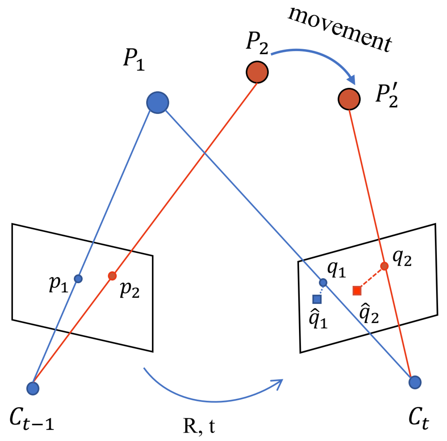
Then, we reproject the feature points of the previous frame to the current frame as illustrated in Figure 5. denote feature points in the previous frame at time , and represent the feature points in the current frame at time t. denote the reprojected points in the current frame matching the feature points . and usually do not coincide because the estimated transformation matrix is inaccurate. Consequently, there will be an offset vector, such as , for each point. The differences in the distance and angle between and are clearly illustrated when the landmark has moved to the position at time t. Figure 6a–c show the difference more intuitively between a static area and moving people for three cases. We can see that even if the initial camera pose calculated from the ego-motion estimation module is not completely accurate, the static points and dynamic points still follow the different distributions. This difference in distribution can help us distinguish between these two points.
A weighted average method is proposed to describe the offset vectors in static areas (all other areas except the potentially dynamic masks in the image), which obtain an adaptive threshold used to distinguish dynamic points. The set of offset vectors in static areas is denoted as . First, we calculate the angle and modulo value for each vector of this set. Then, indicators and are constructed as follows:
the mean value of is denoted as :
denotes the set of offset vectors in potentially moving areas, and represents the corresponding feature point set. For each offset vector in , we calculate and compare it with . The following inequalities are used to determine which point is dynamic:
The results of dynamic point extraction are illustrated in Figure 6d–f. We can see that the points above the moving people are divided into dynamic points (red points). Most of the points on the sitting people are divided into static points (green points) because of the inconspicuous motion.
In the monocular case, we simply use the epipolar constraint to extract dynamic points. The epipolar constraint can be expressed by the following equation:
where F denotes the fundamental matrix, and denote the matched feature points in the current frame and previous frame. For each point of the current frame, we calculate its distance to the corresponding epipolar line . The distance is determined as follows:
where D represents the distance. If the distance exceeds the preset threshold value, then we regard this point as a dynamic point.
Finally, if a certain number of dynamic points fall in the potentially moving area, then the corresponding object is determined to be moving. We discard all feature points located in the contour that are extracted from the image pyramid.
As mentioned in Section 2, there are also some approaches to use semantic segmentation network and geometry-based methods to solve dynamic environment problems like DS-SLAM [35], DynaSLAM [36]. Compared to these two methods, our proposed method has two advantages:
- DS-SLAM only takes the human as a typical representative of dynamic objects in experiments and cannot process stereo sensors data. We predefine 20 categories as potentially dynamic or movable in DM-SLAM and evaluate our system in the pubic monocular, stereo, and RGB-D datasets. DM-SLAM is applicable to a wider range of scenarios.
- DynaSLAM directly regards the segmented content as dynamic and does not extract feature points on them, which is not in line with the real situation (e.g., a parked car). Then, they only extract dynamic points in the RGB-D case using multi-view geometry. In our system, a mask motion discrimination module is added to avoid the problem of discarding too many points on a static mask, causing too few remaining static points. Thus, it has better robustness than the method of directly removing all feature points in the mask.
4. Experimental Results
In this section, we present the experimental results of DM-SLAM on the public datasets TUM RGB-D and KITTI. To demonstrate the improvement of DM-SLAM in dynamic scenes, we compare it with the state-of-the-art visual SLAM systems, i.e., DS-SLAM [34], DynaSLAM [36] and ORB-SLAM2 [3]. A PC with an Intel i7 CPU, 12 GB RAM and a single GeForce GTX 1080 Ti GPU is used to run the programs.
4.1. TUM Dataset
The TUM RGB-D dataset [42] provides color and depth images along with the accurate ground-truth trajectories and contains 39 sequences in different indoor environments. According to whether there are dynamic objects in the scene, we divide the sequences into static scenes and dynamic scenes. According to the magnitude of the motion of dynamic objects, we further divide the dynamic scenes into low-dynamic scenes and high-dynamic scenes. In the sitting sequences, two people are chatting and gesturing in front of a table. We consider the sitting sequences as low-dynamic scenes. In the walking sequences, two people walk back and forth and sit down in front of the desk. We consider the walking sequences as high-dynamic scenes. There are four types of camera motion: (1) halfsphere: the camera moves following the trajectory of a 1-meter diameter halfsphere, (2) xyz: the camera moves along the x–y–z axes, (3) rpy: the camera rotates along the roll, pitch and yaw axes, and (4) static: the camera is roughly kept static manually.
For the sake of brevity, we use the terms fr, half, w, s, d, v to represent freiburg, halfsphere, walking, sitting, desk, and validation in the names of the sequences.
4.1.1. RGB-D
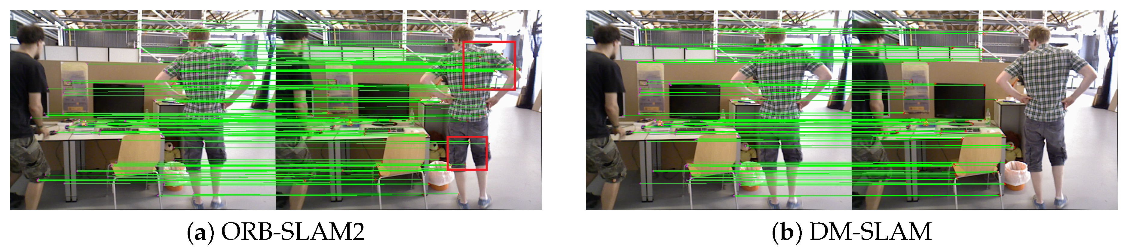
We utilize the metric Absolute Trajectory Error (ATE) [42] for quantitative evaluation, as shown in Table 1. The sequence names are shown in the first column, for example, fr3/w/xyz represents the freiburg3/walking/xyz sequence in the TUM RGB-D dataset. Figure 7 shows the feature extraction and matching results of the fr3/w/xyz sequence in the high-dynamic scenes. As we can see, DM-SLAM can eliminate the influence of the walking people in the red area. Meanwhile, the ORB-SLAM2, DS-SLAM and DynaSLAM systems are used for comparative analysis of trajectory accuracy. For comparison purposes, we present the values of the Root Mean Squared Error (RMSE) [42] of ATE. The improvement values of the RMSE and Standard Deviation (STD) compared to ORB-SLAM2 are also shown in the last column. The values of improvement are defined as follows:
where denotes the improvement value, represents the RMSE value of DM-SLAM, and represents the RMSE value of ORB-SLAM2. Here, we only calculate the improvement compared to the ORB-SLAM2 system.
As we can see in Table 1, the average of RMSE improvement values for high-dynamic scenes is 96.27%. In high-dynamic scenes, DM-SLAM eliminates the influence of dynamic objects in pose estimation. The performance of DM-SLAM has an order of magnitude improvement compared to ORB-SLAM2. However, for the low-dynamic scenes, DM-SLAM only achieves a 20.19% average RMSE improvement. Our method provides less improvement in low-dynamic cases. We think that the reason is that the moving object has a small amplitude of motion in the low-dynamic scenes, and the original ORB-SLAM2 can remove the relatively few points as outliers. For example, in the fr3/s/rpy sequence, two people are seated in a fixed place while gesturing. The dynamic feature points that fall on the arm do not significantly affect the camera pose estimation.
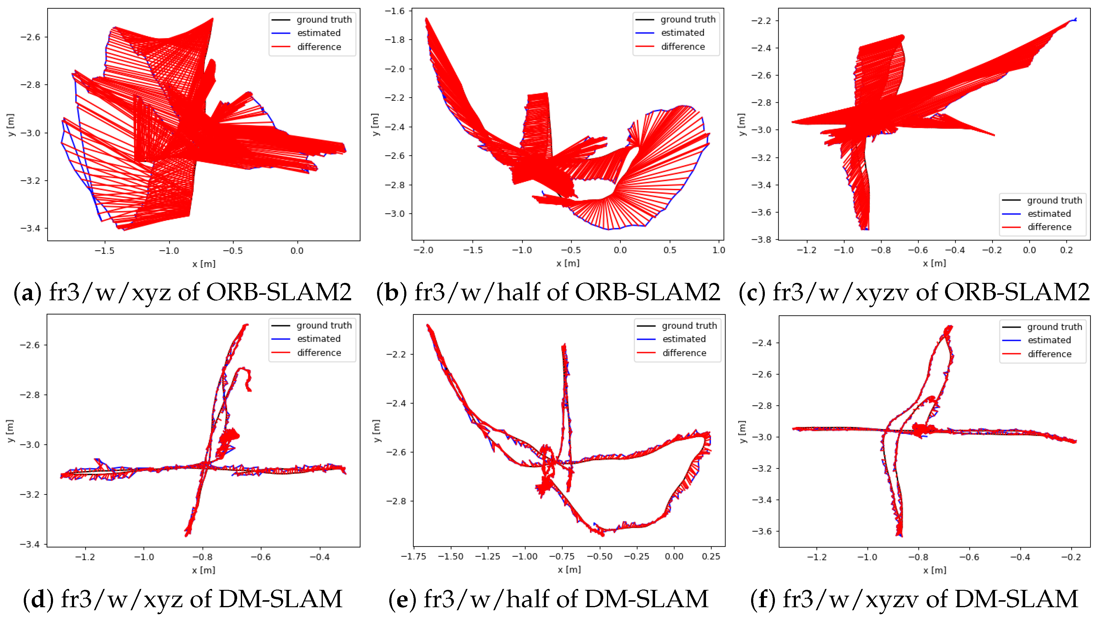
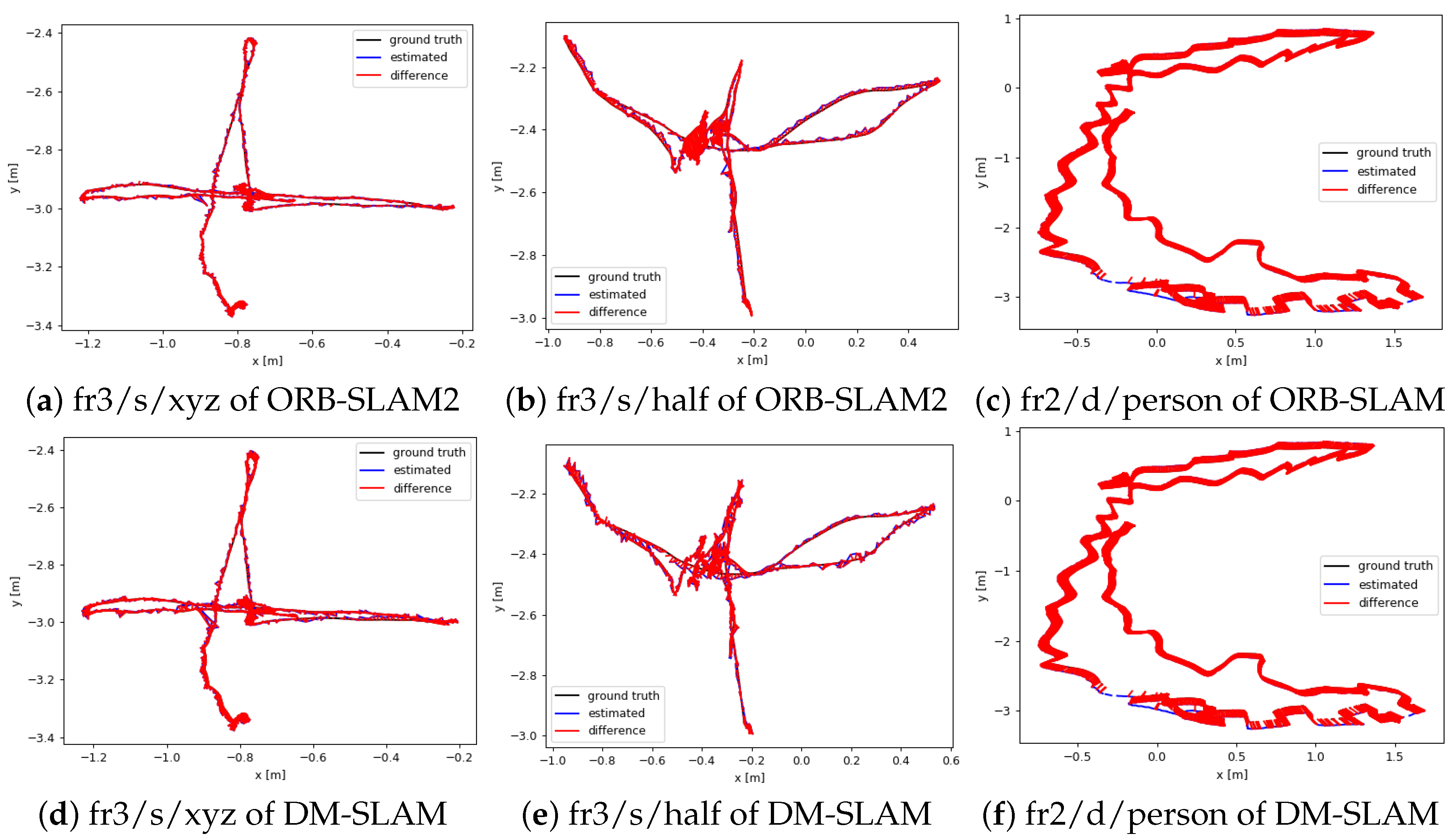
Figure 8 and Figure 9 show the motion trajectory of ORB-SLAM2 and DM-SLAM with reference to the ground truth in the six sequences. Figure 8 shows selected ATE plots for high-dynamic scenes. The accuracy of the trajectory is significantly improved in DM-SLAM because DM-SLAM can estimate the camera poses accurately by eliminating the negative effects of dynamic objects. Figure 9 shows selected ATE plots for low-dynamic scenes. The original ORB-SLAM2 algorithm can also provide good performance for these scenes. The improvement of DM-SLAM is not obvious compared to the high-dynamic scenes.
4.1.2. Monocular
We also conducted experiments on the monocular images in the TUM dataset. The experimental results are shown in Table 2. Compared with Table 1, we can see that ORB-SLAM [7] can achieve more accurate results than in the RGB-D case. The reason is that the monocular initialization algorithm has more stringent restrictions than in the RGB-D case. ORB-SLAM can only be successfully initialized after satisfying the matching and parallax conditions. Therefore, it may take a long time to initialize in dynamic scenes. However, the initialization in DM-SLAM is always quicker than that in ORB-SLAM due to the elimination of the effects of dynamic objects. The percentage of the tracked trajectory in Table 2 is the ratio of successfully tracked frames to the total number of images. This value demonstrate DM-SLAM tends to have a longer trajectory than ORB-SLAM.
In some sequences, the accuracy of ORB-SLAM is slightly higher than that of DM-SLAM. The reason is that the estimated trajectory in DM-SLAM is longer than ORB-SLAM, and there is room for accumulating errors. In general, compared to ORB-SLAM, DM-SLAM initialization creates a map without dynamic objects and has more trajectory information, which is more helpful for subsequent information reuse (e.g., reconstruction of dense map).
4.2. KITTI Dataset
The KITTI dataset [43] is a computer vision algorithm evaluation dataset for autonomous driving scenarios. It contains stereo image data collected from scenes such as urban, rural, and highway. To show the removal effect of dynamic points more intuitively, we implement pose tracking experiments on the KITTI dataset. Figure 10 shows the feature points tracked by DM-SLAM and the ORB-SLAM2 system during pose estimation. DM-SLAM does not track the feature points on the moving cars or bicycles during camera pose estimation, so the influence of the dynamic objects can be eliminated.
Then, we implement trajectory accuracy analysis of the stereo camera in the 11 sequences. Table 3 shows the experimental results of DM-SLAM, compared against those of ORB-SLAM2 and DynaSLAM. We use the absolute trajectory RMSE as the error metric. As we can see, in most sequences that contain a certain number of moving objects, such as cars and bicycles, DM-SLAM can achieve higher tracking accuracy by eliminating the influence of dynamic objects in the road. Nevertheless, in some sequences, most of the recorded cars are parked next to the road, and the position accuracy of our method is slightly lower than that of ORB-SLAM2. The reason is that the most potentially dynamic regions (e.g., parked cars) produced by Mask R-CNN are hence static. The initial ego-motion calculated with the distant points has errors after all the static points in these regions are removed. Then, some of the static points are mistaken as dynamic in the dynamic point extraction module, which will not be used for tracking and mapping, resulting in a slight decrease in tracking accuracy.
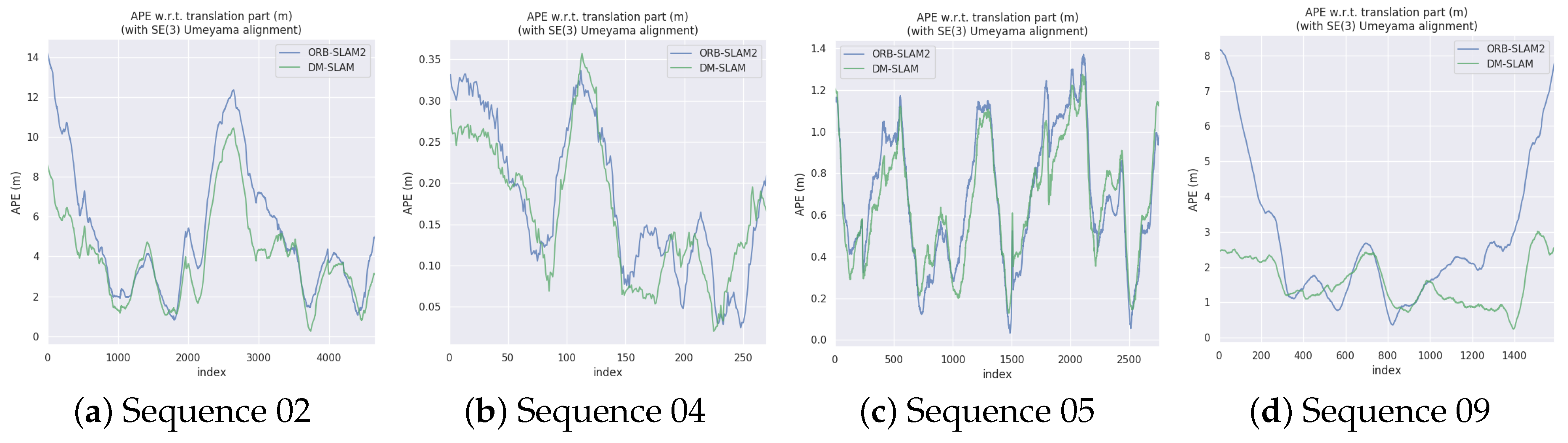
Furthermore, we utilize the evo tool (https://github.com/MichaelGrupp/evo) to plot the absolute pose error (APE) and the motion trajectory of the four sequences in Figure 11 and Figure 12. Since the absolute trajectory error of DynaSLAM is similar to that of ORB-SLAM2, we no longer draw its APE. The APE distribution of DM-SLAM and ORB-SLAM2 is shown in Figure 11. We use SE (3) to align the motion trajectory with the ground-truth trajectory. As we can see, the pose error of DM-SLAM is significantly lower than that of ORB-SLAM2. Figure 12 illustrates the motion trajectories of DM-SLAM with reference to the ground truth. It can be seen that the area with larger error is basically distributed at the corner of the trajectory. Overall, the trajectory of DM-SLAM is consistent with the ground truth and has high accuracy.
4.3. Runtime Analysis
To ensure the integrity of the experiments, Table 4 shows the runtime analysis of DM-SLAM for its different stages, running on the TUM and KITTI datasets. All the experiments are run on a computer with an Intel i7 CPU, 12 GB RAM, and a single GeForce GTX 1080 Ti GPU, and the operating system is Ubuntu 16.04.
We calculate the average time on the TUM and KITTI datasets of different components. The semantic segmentation module is the most time consuming because of the addition of Mask R-CNN. There are two solutions to address this problem in the future. One is to replace Mask R-CNN with a more lightweight semantic segmentation network. Another more efficient way is to deploy the semantic segmentation module on a server with a better hardware configuration and transfer the semantic results to a local terminal. We believe that the SLAM model of cloud terminal collaboration will be more popular in the future.
5. Conclusions
In this paper, a visual SLAM method combining optical flow and a semantic mask is proposed, which can provide good performance in high-dynamic environments for RGB-D, stereo, and monocular cameras. This method can be divided into four modules: semantic segmentation, ego-motion estimation, dynamic point detection, and a feature-based SLAM framework. Our method adds a front-end stage to ORB-SLAM2 to filter out data associated with dynamic objects. In RGB-D/stereo cases, we utilize the reprojection information of feature points to construct an adaptive indicator, which is used to distinguish the dynamic points. In the monocular case, we simply use the epipolar constraint to extract dynamic points.
On the TUM RGB-D dataset, DM-SLAM exhibits an order of magnitude improvement compared to ORB-SLAM2 in high-dynamic scenes. In the monocular case, the accuracy of our approach is similar to that of ORB-SLAM; however, our approach obtains more trajectory and map information. On the KITTI dataset, DM-SLAM achieves higher tracking accuracy for most sequences, except for those containing many static potentially moving objects (e.g., parked cars). To overcome this problem, in future work, we would like to utilize a more accurate mathematical model to describe the distribution of reprojection offset vectors in the a priori static areas, rather than an adaptive threshold. In addition, DM-SLAM uses features tracked in rigid static scenes to estimate camera pose. If all the scenes are dynamic, our current method cannot obtain accurate results due to the lack of static features. In the follow-up work, we will utilize the information on dynamic objects to assist in motion estimation and real-time reconstruction.
Author Contributions
Conceptualization, Junhao Cheng; Formal analysis, Junhao Cheng and Zhi Wang; Methodology, Junhao Cheng and Li Li; Software, Hongyan Zhou; Supervision, Jian Yao; Validation, Li Li and Zhi Wang. Writing—original draft, Junhao Cheng and Hongyan Zhou; Writing—review and editing, Junhao Cheng and Li Li. All authors have read and agree to the published version of the manuscript.
Funding
This work was partially supported by the National Key Research and Development Program of China (Project No. 2017YFB1302400), the National Natural Science Foundation of China (Project No. 41571436), and the Hubei Province Science and Technology Support Program, China (Project No. 2015BAA027).
Conflicts of Interest
The authors declare no conflict of interest.
References
- Newcombe, R.A.; Lovegrove, S.J.; Davison, A.J. DTAM: Dense tracking and mapping in real-time. In Proceedings of the 2011 International Conference on Computer Vision, Barcelona, Spain, 6–13 November 2011; pp. 2320–2327. [Google Scholar]
- Engel, J.; Schöps, T.; Cremers, D. LSD-SLAM: Large-scale direct monocular SLAM. In Proceedings of the European Conference on Computer Vision, Zurich, Switzerland, 6–12 September 2014; Springer: Cham, Switzerland, 2014; pp. 834–849. [Google Scholar]
- Mur-Artal, R.; Tardós, J.D. ORB-SLAM2: An Open-Source SLAM System for Monocular, Stereo and RGB-D Cameras. IEEE Trans. Robot. 2017, 33, 1255–1262. [Google Scholar] [CrossRef] [Green Version]
- Fischler, M.A.; Bolles, R.C. Random sample consensus: A paradigm for model fitting with applications to image analysis and automated cartography. Commun. ACM 1981, 24, 381–395. [Google Scholar] [CrossRef]
- Bloesch, M.; Omari, S.; Hutter, M.; Siegwart, R. Robust visual inertial odometry using a direct EKF-based approach. In Proceedings of the 2015 IEEE/RSJ International Conference on Intelligent Robots and Systems (IROS), Hamburg, Germany, 28 September–2 October 2015; pp. 298–304. [Google Scholar]
- Klein, G.; Murray, D. Parallel tracking and mapping for small AR workspaces. In Proceedings of the 2007 6th IEEE and ACM International Symposium on Mixed and Augmented Reality, Nara, Japan, 13–16 November 2007; pp. 1–10. [Google Scholar]
- Mur-Artal, R.; Montiel, J.M.M.; Tardos, J.D. ORB-SLAM: A versatile and accurate monocular SLAM system. IEEE Trans. Robot. 2015, 31, 1147–1163. [Google Scholar] [CrossRef] [Green Version]
- Stühmer, J.; Gumhold, S.; Cremers, D. Real-time dense geometry from a handheld camera. In Proceedings of the Joint Pattern Recognition Symposium, Darmstadt, Germany, 22–24 September 2010; Springer: Berlin/Heidelberg, Germany, 2010; pp. 11–20. [Google Scholar]
- Graber, G.; Pock, T.; Bischof, H. Online 3D reconstruction using convex optimization. In Proceedings of the 2011 IEEE International Conference on Computer Vision Workshops (ICCV Workshops), Barcelona, Spain, 6–13 November 2011; pp. 708–711. [Google Scholar]
- Engel, J.; Koltun, V.; Cremers, D. Direct sparse odometry. IEEE Trans. Pattern Anal. Mach. Intell. 2017, 40, 611–625. [Google Scholar] [CrossRef] [PubMed]
- Saputra, M.R.U.; Markham, A.; Trigoni, N. Visual SLAM and structure from motion in dynamic environments: A survey. ACM Comput. Surv. (CSUR) 2018, 51, 37. [Google Scholar] [CrossRef]
- Sun, Y.; Liu, M.; Meng, M.Q.H. Improving RGB-D SLAM in dynamic environments: A motion removal approach. Robot. Auton. Syst. 2017, 89, 110–122. [Google Scholar] [CrossRef]
- Li, S.; Lee, D. RGB-D SLAM in dynamic environments using static point weighting. IEEE Robot. Autom. Lett. 2017, 2, 2263–2270. [Google Scholar] [CrossRef]
- Wang, Y.; Huang, S. Towards dense moving object segmentation based robust dense RGB-D SLAM in dynamic scenarios. In Proceedings of the 2014 13th International Conference on Control Automation Robotics & Vision (ICARCV), Singapore, 10–12 December 2014; pp. 1841–1846. [Google Scholar]
- Alcantarilla, P.F.; Yebes, J.J.; Almazán, J.; Bergasa, L.M. On combining visual SLAM and dense scene flow to increase the robustness of localization and mapping in dynamic environments. In Proceedings of the 2012 IEEE International Conference on Robotics and Automation, Saint Paul, MN, USA, 14–18 May 2012; pp. 1290–1297. [Google Scholar]
- Tan, W.; Liu, H.; Dong, Z.; Zhang, G.; Bao, H. Robust monocular SLAM in dynamic environments. In Proceedings of the 2013 IEEE International Symposium on Mixed and Augmented Reality (ISMAR), Adelaide, SA, Australia, 1–4 October 2013; pp. 209–218. [Google Scholar]
- Shimamura, J.; Morimoto, M.; Koike, H. Robust vSLAM for Dynamic Scenes. In Proceedings of the MVA2011 IAPR Conference on Machine Vision Applications, Nara, Japan, 13–15 June 2011; pp. 344–347. [Google Scholar]
- Scaramuzza, D.; Fraundorfer, F.; Siegwart, R. Real-time monocular visual odometry for on-road vehicles with 1-point ransac. In Proceedings of the 2009 IEEE International Conference on Robotics and Automation, Kobe, Japan, 12–17 May 2009; pp. 4293–4299. [Google Scholar]
- Ferrera, M.; Moras, J.; Trouvé-Peloux, P.; Creuze, V. Real-Time Monocular Visual Odometry for Turbid and Dynamic Underwater Environments. Sensors 2019, 19, 687. [Google Scholar] [CrossRef] [PubMed] [Green Version]
- Liu, G.; Zeng, W.; Feng, B.; Xu, F. DMS-SLAM: A General Visual SLAM System for Dynamic Scenes with Multiple Sensors. Sensors 2019, 19, 3714. [Google Scholar] [CrossRef] [PubMed] [Green Version]
- Bian, J.; Lin, W.Y.; Matsushita, Y.; Yeung, S.K.; Nguyen, T.D.; Cheng, M.M. Gms: Grid-based motion statistics for fast, ultra-robust feature correspondence. In Proceedings of the IEEE Conference on Computer Vision and Pattern Recognition, Honolulu, HI, USA, 21–26 July 2017; pp. 4181–4190. [Google Scholar]
- Jones, E.S.; Soatto, S. Visual-inertial navigation, mapping and localization: A scalable real-time causal approach. Int. J. Robot. Res. 2011, 30, 407–430. [Google Scholar] [CrossRef]
- Leutenegger, S.; Furgale, P.; Rabaud, V.; Chli, M.; Konolige, K.; Siegwart, R. Keyframe-based visual-inertial slam using nonlinear optimization. Int. J. Robot. Res. 2015, 34, 314–334. [Google Scholar] [CrossRef] [Green Version]
- Kim, D.H.; Han, S.B.; Kim, J.H. Visual odometry algorithm using an RGB-D sensor and IMU in a highly dynamic environment. In Robot Intelligence Technology and Applications 3; Springer: Cham, Switzerland, 2015; pp. 11–26. [Google Scholar]
- Agudo, A.; Moreno-Noguer, F.; Calvo, B.; Montiel, J.M.M. Sequential non-rigid structure from motion using physical priors. IEEE Trans. Pattern Anal. Mach. Intell. 2015, 38, 979–994. [Google Scholar] [CrossRef] [PubMed] [Green Version]
- Agudo, A.; Moreno-Noguer, F.; Calvo, B.; Montiel, J. Real-time 3D reconstruction of non-rigid shapes with a single moving camera. Comput. Vis. Image Underst. 2016, 153, 37–54. [Google Scholar] [CrossRef] [Green Version]
- Tateno, K.; Tombari, F.; Laina, I.; Navab, N. Cnn-slam: Real-time dense monocular slam with learned depth prediction. In Proceedings of the IEEE Conference on Computer Vision and Pattern Recognition, Honolulu, HI, USA, 21–26 July 2017; pp. 6243–6252. [Google Scholar]
- DeTone, D.; Malisiewicz, T.; Rabinovich, A. Toward geometric deep SLAM. arXiv 2017, arXiv:1707.07410. [Google Scholar]
- Bowman, S.L.; Atanasov, N.; Daniilidis, K.; Pappas, G.J. Probabilistic data association for semantic slam. In Proceedings of the 2017 IEEE International Conference on Robotics and Automation (ICRA), Singapore, 29 May–3 June 2017; pp. 1722–1729. [Google Scholar]
- Lianos, K.N.; Schonberger, J.L.; Pollefeys, M.; Sattler, T. Vso: Visual semantic odometry. In Proceedings of the European Conference on Computer Vision (ECCV), Munich, Germany, 8–14 September 2018; pp. 234–250. [Google Scholar]
- Riazuelo, L.; Montano, L.; Montiel, J. Semantic visual SLAM in populated environments. In Proceedings of the 2017 European Conference on Mobile Robots (ECMR), Paris, France, 6–8 September 2017; pp. 1–7. [Google Scholar]
- Vineet, V.; Miksik, O.; Lidegaard, M.; Nießner, M.; Golodetz, S.; Prisacariu, V.A.; Kähler, O.; Murray, D.W.; Izadi, S.; Pérez, P.; et al. Incremental dense semantic stereo fusion for large-scale semantic scene reconstruction. In Proceedings of the 2015 IEEE International Conference on Robotics and Automation (ICRA), Seattle, WA, USA, 26–30 May 2015; pp. 75–82. [Google Scholar]
- Kaneko, M.; Iwami, K.; Ogawa, T.; Yamasaki, T.; Aizawa, K. Mask-SLAM: Robust feature-based monocular SLAM by masking using semantic segmentation. In Proceedings of the IEEE Conference on Computer Vision and Pattern Recognition Workshops, Salt Lake City, UT, USA, 18–22 June 2018; pp. 258–266. [Google Scholar]
- Yu, C.; Liu, Z.; Liu, X.J.; Xie, F.; Yang, Y.; Wei, Q.; Fei, Q. Ds-slam: A semantic visual slam towards dynamic environments. In Proceedings of the 2018 IEEE/RSJ International Conference on Intelligent Robots and Systems (IROS), Madrid, Spain, 1–5 October 2018; pp. 1168–1174. [Google Scholar]
- Badrinarayanan, V.; Kendall, A.; Cipolla, R. Segnet: A deep convolutional encoder-decoder architecture for image segmentation. IEEE Trans. Pattern Anal. Mach. Intell. 2017, 39, 2481–2495. [Google Scholar] [CrossRef]
- Bescos, B.; Fácil, J.M.; Civera, J.; Neira, J. DynaSLAM: Tracking, mapping, and inpainting in dynamic scenes. IEEE Robot. Autom. Lett. 2018, 3, 4076–4083. [Google Scholar] [CrossRef] [Green Version]
- He, K.; Gkioxari, G.; Dollár, P.; Girshick, R. Mask r-cnn. In Proceedings of the IEEE International Conference on Computer Vision, Venice, Italy, 22–29 October 2017; pp. 2961–2969. [Google Scholar]
- Bahraini, M.S.; Rad, A.B.; Bozorg, M. SLAM in Dynamic Environments: A Deep Learning Approach for Moving Object Tracking Using ML-RANSAC Algorithm. Sensors 2019, 19, 3699. [Google Scholar] [CrossRef] [Green Version]
- Girshick, R. Fast r-cnn. In Proceedings of the IEEE International Conference on Computer Vision, Santiago, Chile, 7–13 December 2015; pp. 1440–1448. [Google Scholar]
- Lin, T.Y.; Maire, M.; Belongie, S.; Hays, J.; Perona, P.; Ramanan, D.; Dollár, P.; Zitnick, C.L. Microsoft coco: Common objects in context. In Proceedings of the European Conference on Computer Vision, Zurich, Switzerland, 6–12 September 2014; Springer: Cham, Switzerland, 2014; pp. 740–755. [Google Scholar]
- Baker, S.; Matthews, I. Lucas-kanade 20 years on: A unifying framework. Int. J. Comput. Vis. 2004, 56, 221–255. [Google Scholar] [CrossRef]
- Sturm, J.; Engelhard, N.; Endres, F.; Burgard, W.; Cremers, D. A benchmark for the evaluation of RGB-D SLAM systems. In Proceedings of the 2012 IEEE/RSJ International Conference on Intelligent Robots and Systems, Vilamoura, Portugal, 7–12 October 2012; pp. 573–580. [Google Scholar]
- Geiger, A.; Lenz, P.; Stiller, C.; Urtasun, R. Vision meets robotics: The KITTI dataset. Int. J. Robot. Res. 2013, 32, 1231–1237. [Google Scholar] [CrossRef] [Green Version]
Figure 1.
Illustration of the graph optimization model in Simultaneous Localization and Mapping (SLAM). The circles represent landmarks. In addition, the triangles represent camera poses. The solid edges link camera poses. The dotted edges link the camera poses and observed landmarks. In (a), the camera poses are estimated normally when all of the landmarks are static. In (b), the landmark has moved to the position at the next moment. Red triangles and lines represent the pose error and constraints obtained with dynamic objects. The interference of dynamic objects is clearly illustrated by comparing the two situations.

Figure 2.
Overview of our proposed method. Input frames are segmented by the Mask R-CNN network, and then the feature points that fall in the initially assumed dynamic content are discarded for ego-motion estimation. The static feature points left are fed into the SLAM algorithm for tracking and mapping after dynamic feature points are discarded.

Figure 3.
Detailed framework of our proposed method. We add a front-end stage to the ORB-SLAM2 framework as illustrated in the figure. A low-cost tracking algorithm is needed to calculate the initial ego-motion after the Mask R-CNN module. Then, there are two different strategies to extract dynamic feature points for monocular and RGB-D/stereo cases. We discriminate which masks are dynamic so that all feature points in the corresponding dynamic content can be discarded.
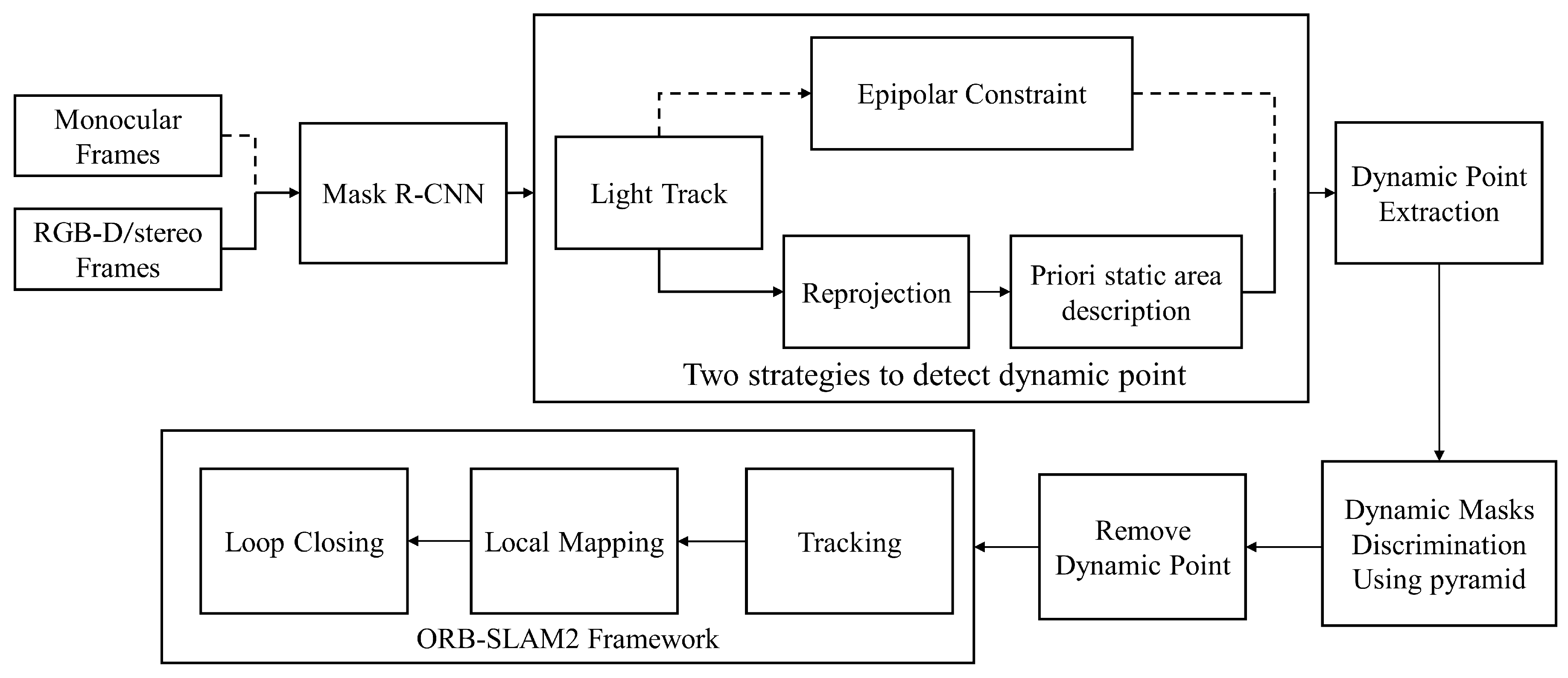
Figure 4.
(a) The pixel-wise semantic segmentation of the RGB image. Different color areas represent different instances; (b) potentially dynamic objects areas. We extract the two instances named “person” in (a) as potentially dynamic objects.
Figure 4.
(a) The pixel-wise semantic segmentation of the RGB image. Different color areas represent different instances; (b) potentially dynamic objects areas. We extract the two instances named “person” in (a) as potentially dynamic objects.

Figure 5.
Different offset vectors of static points and dynamic points. and denote the camera center position at different times. and represent the offset vectors of static point and dynamic point in the current frame.
Figure 5.
Different offset vectors of static points and dynamic points. and denote the camera center position at different times. and represent the offset vectors of static point and dynamic point in the current frame.

Figure 6.
(a–c) Three cases for object motion. The yellow line between the red and green endpoints in the figure is the offset vector in Figure 5; (d–f) dynamic point extraction results of (a–c). Static feature points are displayed in green, and dynamic points are displayed in red. The figure is best viewed in color.
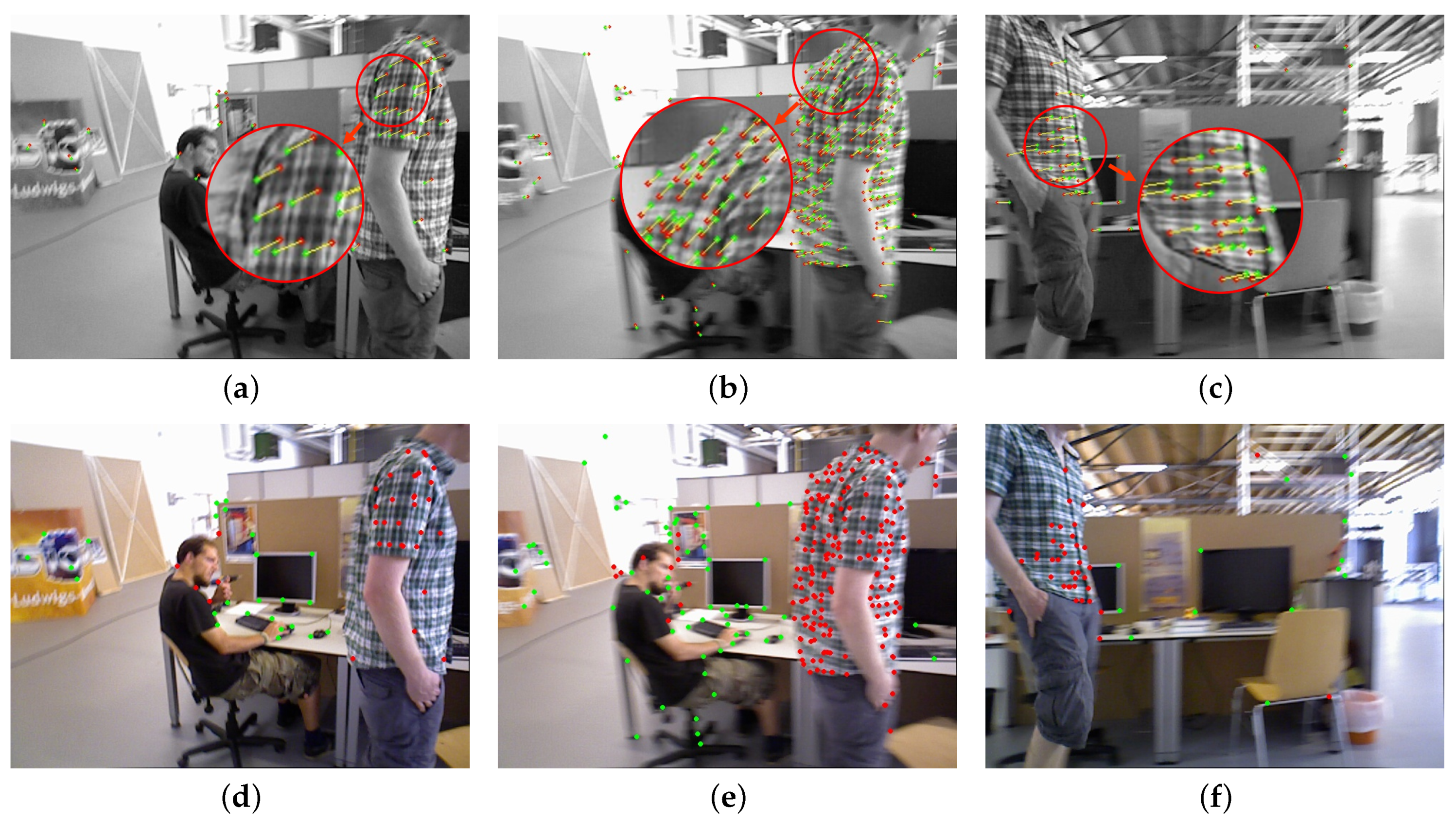
Figure 7.
(a,b) Feature matching results between frames in ORB-SLAM2 and DM-SLAM. The red boxes in the figure represent the dynamic area.
Figure 7.
(a,b) Feature matching results between frames in ORB-SLAM2 and DM-SLAM. The red boxes in the figure represent the dynamic area.

Figure 8.
Plots of the ATE [m] for high-dynamic scenes: fr3/w/xyz, fr3/w/half, fr3/w/xyzv. (a–c) the experiments performed with ORB-SLAM2; (d–f) the experiments performed with DM-SLAM.
Figure 8.
Plots of the ATE [m] for high-dynamic scenes: fr3/w/xyz, fr3/w/half, fr3/w/xyzv. (a–c) the experiments performed with ORB-SLAM2; (d–f) the experiments performed with DM-SLAM.

Figure 9.
Plots of the ATE [m] for low-dynamic scenes: fr3/s/xyz, fr3/s/half, fr2/d/person; (a–c) the experiments performed with ORB-SLAM2; (d–f) the experiments performed with DM-SLAM.
Figure 9.
Plots of the ATE [m] for low-dynamic scenes: fr3/s/xyz, fr3/s/half, fr2/d/person; (a–c) the experiments performed with ORB-SLAM2; (d–f) the experiments performed with DM-SLAM.

Figure 10.
Tracking experiments with ORB-SLAM2 and DM-SLAM on the 01, 02, 08, and 09 sequences. The rectangular boxes represent the moving objects, and there are some feature points tracked in the red box of ORB-SLAM2 but not in the yellow box of DM-SLAM.
Figure 10.
Tracking experiments with ORB-SLAM2 and DM-SLAM on the 01, 02, 08, and 09 sequences. The rectangular boxes represent the moving objects, and there are some feature points tracked in the red box of ORB-SLAM2 but not in the yellow box of DM-SLAM.
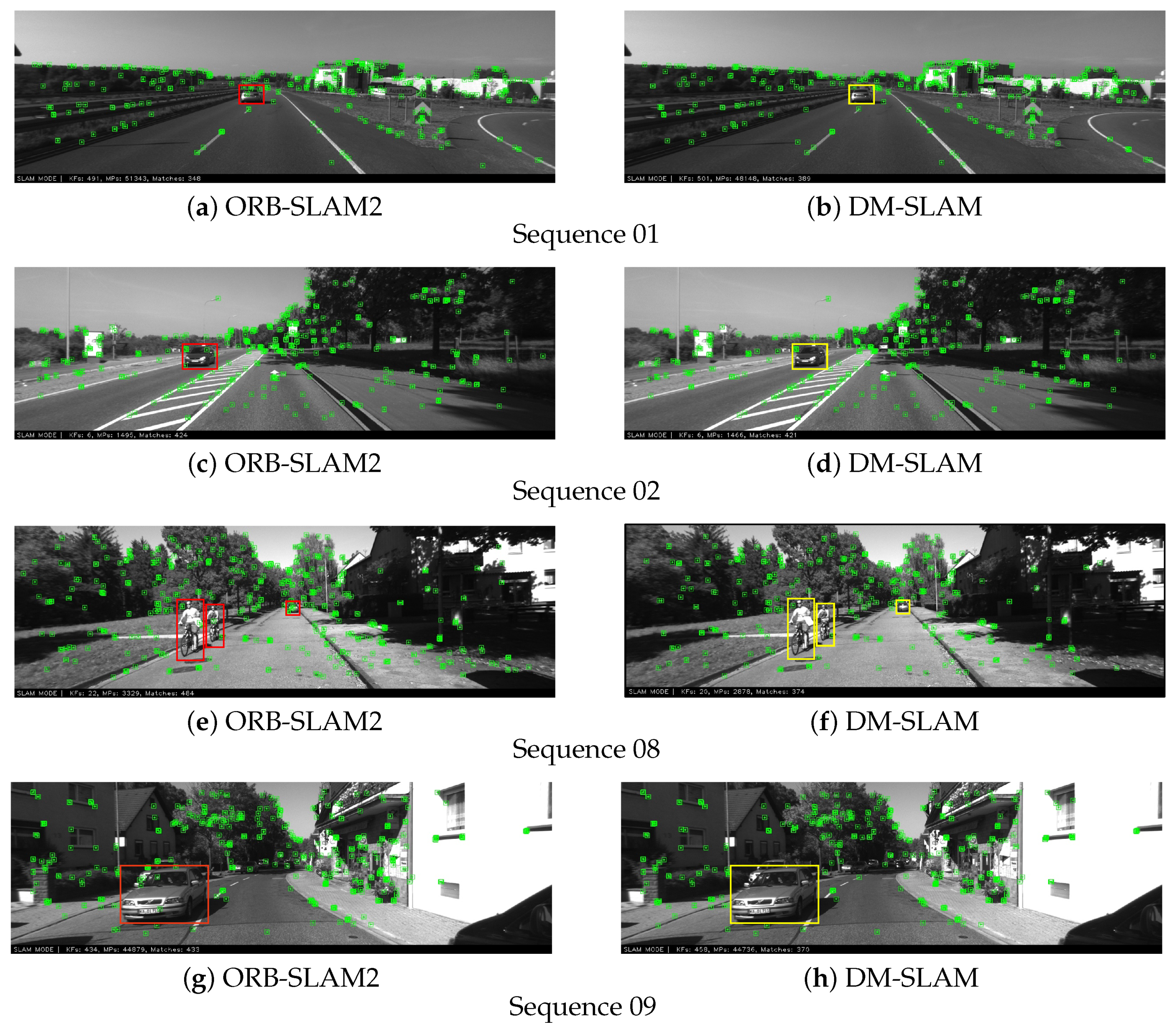
Figure 11.
(a–d) Absolute pose error (APE) of DM-SLAM and ORB-SLAM2 for the 02, 04, 05, and 09 sequences of the KITTI dataset.
Figure 11.
(a–d) Absolute pose error (APE) of DM-SLAM and ORB-SLAM2 for the 02, 04, 05, and 09 sequences of the KITTI dataset.

Figure 12.
(a–d) Comparison of the motion trajectories of DM-SLAM with the ground-truth trajectories for the 02, 04, 05, and 09 sequences of the KITTI dataset. The dotted line represents the ground-truth trajectory. The degree of warmth and coldness of the color on the dotted line represents the magnitude of the error.


Table 1.
Quantitative comparison results of the absolute trajectory error (ATE) [m] in meters for the experiments. It can be seen that our method exhibits significantly improved performance compared to ORB-SLAM2 in high-dynamic scenes in terms of the ATE.
Table 1.
Quantitative comparison results of the absolute trajectory error (ATE) [m] in meters for the experiments. It can be seen that our method exhibits significantly improved performance compared to ORB-SLAM2 in high-dynamic scenes in terms of the ATE.
| Sequences | ORB-SLAM2 | DS-SLAM | DynaSLAM | DM-SLAM | Improvement | |||
|---|---|---|---|---|---|---|---|---|
| RMSE [m] | STD [m] | RMSE [m] | RMSE [m] | RMSE [m] | STD [m] | RMSE [%] | STD [%] | |
| fr3/w/xyz | 0.7137 | 0.3584 | 0.0241 | 0.0158 | 0.0148 | 0.0072 | 97.93% | 97.99% |
| fr3/w/rpy | 0.8357 | 0.4169 | 0.3741 | 0.0402 | 0.0328 | 0.0194 | 96.08% | 95.35% |
| fr3/w/static | 0.3665 | 0.1448 | 0.0081 | 0.0080 | 0.0079 | 0.0040 | 97.84% | 97.24% |
| fr3/w/half | 0.4068 | 0.1698 | 0.0282 | 0.0276 | 0.0274 | 0.0137 | 93.26% | 91.93% |
| fr3/s/static | 0.0092 | 0.0039 | 0.0061 | 0.0064 | 0.0063 | 0.0032 | 31.52% | 17.95% |
| fr3/s/rpy | 0.0245 | 0.0172 | 0.0187 | 0.0302 | 0.0230 | 0.0134 | 6.12% | 22.09% |
| fr3/s/half | 0.0231 | 0.0112 | 0.0148 | 0.0191 | 0.0178 | 0.0103 | 22.94% | 30.41% |
Table 2.
Comparison of the RMSE of the ATE [m] and percentage of tracked trajectory for monocular cameras.
Table 2.
Comparison of the RMSE of the ATE [m] and percentage of tracked trajectory for monocular cameras.
| Sequences | ATE RMSE [m] | Traj (%) | ||||
|---|---|---|---|---|---|---|
| ORB-SLAM2 | DynaSLAM | DM-SLAM | ORB-SLAM2 | DynaSLAM | DM-SLAM | |
| fr3/w/xyz | 0.014 | 0.014 | 0.020 | 85.61 | 87.37 | 97.90 |
| fr3/w/half | 0.017 | 0.021 | 0.024 | 90.12 | 97.84 | 97.87 |
| fr3/w/rpy | 0.066 | 0.052 | 0.050 | 85.82 | 85.11 | 87.24 |
| fr3/w/static | 0.005 | 0.004 | 0.004 | 89.30 | 90.01 | 91.57 |
| fr3/s/xyz | 0.008 | 0.013 | 0.014 | 95.47 | 95.51 | 95.78 |
| fr3/s/rpy | 0.042 | 0.021 | 0.021 | 80.36 | 54.39 | 92.54 |
Table 3.
Comparison of the RMSE of the ATE [m] for stereo cameras.
| Sequences | ORB-SLAM2 | DynaSLAM | DM-SLAM |
|---|---|---|---|
| ATE RMSE [m] | ATE RMSE [m] | ATE RMSE [m] | |
| KITTI 00 | 1.3 | 1.4 | 1.4 |
| KITTI 01 | 11.4 | 9.4 | 9.1 |
| KITTI 02 | 6.2 | 6.7 | 4.6 |
| KITTI 03 | 0.6 | 0.6 | 0.6 |
| KITTI 04 | 0.2 | 0.2 | 0.2 |
| KITTI 05 | 0.8 | 0.8 | 0.7 |
| KITTI 06 | 0.8 | 0.8 | 0.8 |
| KITTI 07 | 0.5 | 0.5 | 0.6 |
| KITTI 08 | 3.8 | 3.5 | 3.3 |
| KITTI 09 | 3.4 | 1.6 | 1.7 |
| KITTI 10 | 1.0 | 1.2 | 1.1 |
Table 4.
DM-SLAM average computational time (unit: ms) of different components.
| Datasets | Semantic Segmentation [ms] | Ego-Motion Estimation [ms] | Dynamic Point Detection [ms] |
|---|---|---|---|
| TUM | 201.02 | 3.16 | 40.64 |
| KITTI | 210.11 | 7.03 | 94.59 |
© 2020 by the authors. Licensee MDPI, Basel, Switzerland. This article is an open access article distributed under the terms and conditions of the Creative Commons Attribution (CC BY) license (http://creativecommons.org/licenses/by/4.0/).
Share and Cite
MDPI and ACS Style
Cheng, J.; Wang, Z.; Zhou, H.; Li, L.; Yao, J. DM-SLAM: A Feature-Based SLAM System for Rigid Dynamic Scenes. ISPRS Int. J. Geo-Inf. 2020, 9, 202. https://0-doi-org.brum.beds.ac.uk/10.3390/ijgi9040202
AMA Style
Cheng J, Wang Z, Zhou H, Li L, Yao J. DM-SLAM: A Feature-Based SLAM System for Rigid Dynamic Scenes. ISPRS International Journal of Geo-Information. 2020; 9(4):202. https://0-doi-org.brum.beds.ac.uk/10.3390/ijgi9040202
Chicago/Turabian StyleCheng, Junhao, Zhi Wang, Hongyan Zhou, Li Li, and Jian Yao. 2020. "DM-SLAM: A Feature-Based SLAM System for Rigid Dynamic Scenes" ISPRS International Journal of Geo-Information 9, no. 4: 202. https://0-doi-org.brum.beds.ac.uk/10.3390/ijgi9040202
Note that from the first issue of 2016, this journal uses article numbers instead of page numbers. See further details here.