Spatial Paradigms in Road Networks and Their Delimitation of Urban Boundaries Based on KDE

Abstract

An in-depth analysis of urban road network distribution plays a critical role in understanding the urbanization process. However, effective ways to quantitatively analyze the spatial paradigms of road networks are still lacking, and few studies have utilized road networks to rapidly identify urban areas of a region. Thus, using a fast-developing region in the south-eastern costal region of China, Fuzhou City, as a case, we introduced kernel density estimation (KDE) to characterize road networks and quantified the area’s spatial heterogeneity using exploratory spatial data analysis (ESDA) and semivariance analysis (SA). The results show that there is an uneven spatial distribution of the networks both at the regional and downtown levels. At the regional level, there is a conspicuous polarization in the road distribution, with the KDE being much higher in the urban areas than in the rural areas; at the downtown level, the KDE gradually decreases from the center to the periphery. Quantitatively, the ranges of the spatial dependence of the networks are approximately 25 km for the entire study region and 12 km for the downtown area. Additionally, the spatial variations vary among different directions, with greater variations in the northeast–southwest and the southeast–northwest directions compared with the other directions, which is in line with the urban sprawl policy of the study area. Both the qualitative and quantitative results show that the distribution of road networks has a clear urban–rural dual structure, which indicates that road networks can be an active tool in identifying the urban areas of a region. To this end, we propose a quick and easy method to delimit urban areas using KDE. The extraction results of KDE are better than those of the index-based built-up index (IBI), indicating the effectivity and feasibility of our proposed method to identify the urban areas in the region. This research sheds new light on urbanization development research.

1. Introduction

Urbanization is a fundamentally basic process in human social and economic development, and has an increasingly powerful impact on our society and environment [1]. The United Nations (UN) World Urbanization Prospects estimated 2007 to be the year when, for the first time, more people in the world lived in urban than in rural areas; the proportion of people living in urban areas reached 55% in 2017, and it is projected that 7 billion people, 68% of the world’s population, will live in urban areas by 2050 (https://ourworldindata.org/urbanization). This mass migration of populations from rural to urban areas has led to large-scale urban expansion, mainly in terms of built-up land or impervious surfaces, encroaching many natural landscapes and changing their patterns [2,3]. More than 700,000 km² of land was occupied by cities in the year 2010, and this area is expected to grow to 1.21 million km² by 2030 [4]. In addition, it was reported that even more of Earth’s land surface (approximately 75%) has been modified by humans to support urban residences [5]. This human-induced land cover change has caused considerable global climate change, environmental pollution, and biodiversity loss [6], and has also led to air pollution in urban areas and subsequent health problems for urban residents [3,7]. As such, a deeper understanding of the spatial mechanisms of urbanization is more important than ever. Urban planning and construction are especially needed in landscape management and ecology [8,9]. Among the artificial drivers of the urbanization process, road networks are considered a primary factor in urban expansion, as well as one of the relatively permanent constituent elements of the landscape [10,11]. As a typical network of corridors, roads not only play an indispensable role in the spatial patterns of the urban landscape [12,13], but are also critical for the accompanying social, economic, and ecological processes [10,14], as well as for the progress of urban sprawl [15]. Roads are everywhere in the landscape and affect nearly 20% of a nation’s surface area [10]. As a result, research on quantifying the spatial patterns of road networks has attracted widespread attention from scholars worldwide over the past two decades [16,17]. However, a quantitative analysis of road network distribution in metropolitan areas is still lacking [18]. Few studies use road networks to quickly identify urban boundaries. Thus, quantifying road networks and their applications in dividing the urban periphery may open new windows into urbanization expansion and shed a new light on urban planning and construction, as well as urban sustainability.

A previous study revealed that it is extremely difficult to define the geography of a road network [19] because different road networks display different topologies and geometries in a given geographical range [14]. Networks consist of a set of links (i.e., lines) and nodes (i.e., points). Early studies measuring the structure of a road network date back to the 1960s and have focused mainly on the topological structure of a network using graph-theoretic analyses under restricted situations, such as limited data, limited calculation abilities, and problematic simulation techniques [20]. As travel demand models became more available, studies began to explore the connectivity of road networks, both qualitatively and quantitatively, especially urban highways [11]. More recently, the emphasis of studies on road networks has shifted from topologic and geometrical properties to large-scale statistical characteristics [21]. From a larger regional perspective, the distribution of road networks has distinct local characteristics [22]; for example, road networks in the suburbs or countryside tend to be curved and sparse but are relatively regular and dense in plains, especially in urban areas with high population densities, resulting in more complex road patterns [23]. To this end, it is a challenge and of great importance to effectively measure road networks and their geographical heterogeneity at a broader scale [11].

The density of road networks refers to the value of the total length of roads divided by the area of a certain region [24,25]. Road density, one of the most commonly used indicators in the evaluation of the structures of road networks [23], is also an important symbol of social and economic development levels [11]. It has been used as a proxy for housing density [26], population density [16], and the delimitation of city centers [17,18]. For example, Zhang et al. [17] indicated that the density of road networks, overall, provides accurate information for town centeredness analyses. Therefore, as a feasible indicator, road density has been employed to analyze many social and ecological processes, such as built-up land changes, housing prices, human access, faunal movement, hydrology, and fire and landscape patterns [17,27]. These previous studies revealed that housing density, housing prices, wildlife–vehicle collisions, and landscape fragmentation are positively related to road density, while wetland areas, forest areas, and landscape connectivity are negatively related.

Generally, there are two different methods used to estimate the density of a road network: the grid-based index and kernel density estimation (KDE) [14]. Grid-based road density is easy to calculate, but faces interference from the artificial boundaries of the chosen grid, as well as from orientation and position [14,23], and thus may have an insignificant relationship with natural entities. For example, the relationship between grid-based road density and landscape fragmentation is poor due to the bias of the artificial boundaries of the chosen grid [28]. By contrast, the second method uses KDE to obtain smooth continuous surfaces for road density, thus providing a more consistent analysis that overcomes the restrictions of the arbitrary boundaries of the sample grid. Previous studies have widely applied KDE function to many point-density pattern analyses, such as population density estimation [29], crime hot-spot observation [20], and wildlife activity-range estimation [30]. More recently, KDE has also been used to evaluate road density [14,23]. Overcoming the arbitrariness in the chosen grid size of traditional grid-based density, KDE was proven to provide a more consistent analysis for road networks [14].

Urbanization has become one of the most prominent features of the world since the 20th century [31,32]. However, urban structure studies are highly restricted by urbanization boundary datasets [33]. Conventionally, various statistics, such as gross domestic product (GDP), population number, and industrialization index, have been employed to determine urban boundaries; however, the shortcomings of these methods are obvious due to inconsistent statistical standards and the statistical methods adopted by different regions [34,35]. Recently, with the increased availability of remote sensing data (which has the advantage of constantly updating and providing spatially explicit information), these data have been widely employed to explore urban expansion [36,37]. Among these remote sensing data, Landsat and ASTER data are the most suitable for mesoscale measurements of urban changes [38]. For example, the impervious surface area (ISA) [39], the normalized difference built-up index (NDBI) [40], and index-based built-up index (IBI) [38] retrieved from satellite data have been used to investigate the spatiotemporal patterns of urban development. Nighttime light data have also been widely applied in monitoring urban expansion [36].

Remote sensing data have gradually been accepted for observing urban expansion. However, the pre-processing and extraction processes of remote sensing data are more complicated, and are especially difficult for researchers who do not have knowledge of remote sensing. Therefore, there is an urgent need for a simpler method to extract urban boundaries to supplement the needs of most researchers. More recently, the volunteered geographic information (VGI) collected in OpenStreetMap (OSM) has been used in many applications [41]. The road networks of OSM have been extensively applied in many studies, including autonomous robot navigation [42], road distribution [43], mapping regional landscapes [44], and urban function zoning [45]. Therefore, it is necessary to make full use of these up-to-date road networks to support urban development studies. The road network has an obvious spatial paradigm at the regional and local levels [22]. Road networks vary greatly in their road distribution at the regional level. For example, road distributions range from tight grids of 40 km/km², typical of urban centers in common areas, to less than 0.1 km/km² in steep-terrain areas [23]. Variations in the density of road networks at the local level are an indivisible element of central-place theory [14]. The proportion of land occupied by road networks increases, eventually approximating an urban center, while the proportion decreases with increasing distance from the center. The increase in road density close to the city center occurs because of agglomeration economies and the bid–rent theory, which posits that business and corporate activities (high traffic-generating activities) are willing to pay for good access to the city center to achieve a certain level of utility or profit [14]. When the urban boundary expands at the urban–rural fringe, road networks extend, and rural landscapes are replaced by built-up areas. However, bare agricultural fields can be very similar to built-up areas, thereby creating difficulty in determining urban boundaries [46]. Nevertheless, such areas always have much sparser road networks [26]. On the basis of this feature, coupled with the obvious urban–rural dual structure characteristics of the road network identified by the above analyses, the measurement of KDE may supply additional structural information for the delimitation of urban areas. This idea has already been pursued in previous studies [17,47] that indicated that the information on road density can improve the results of urban–rural segmentation. Following this logic, the road network may be a good surrogate to be quantified and used in the analysis of urbanization development.

Although previous studies have used road network density to delimit urban areas [14,17,47], the employed linear density featured a grid-based index [17,20], which may face interference from the artificial boundaries of the chosen grid, while the KDE-based density is calculated from point datasets (road network junctions) and street numbers in a grid [14]. Moreover, the different bandwidths chosen in a KDE analysis produce different density patterns. However, knowledge of how to utilize a KDE analysis of linear road network data for delimiting urban areas and the choice of an appropriate kernel bandwidth for different sizes of cities is still lacking. Thus, using a fast-developing coastal region of China, Fuzhou City, as a case, we characterized road networks based on KDE function and employed exploratory spatial data analysis (ESDA) and semivariance analysis (SA) to quantify the spatial heterogeneity of the networks. Thus, the purposes of this study were (1) to explore the quantitative characteristics of the spatial variation in the road network using ESDA and SA, and (2) to propose an effective way to quickly identify the urban boundary of a region using KDE as a proxy based on a linear road network dataset. This research will provide a new perspective for urbanization research.

2. Materials and Methods

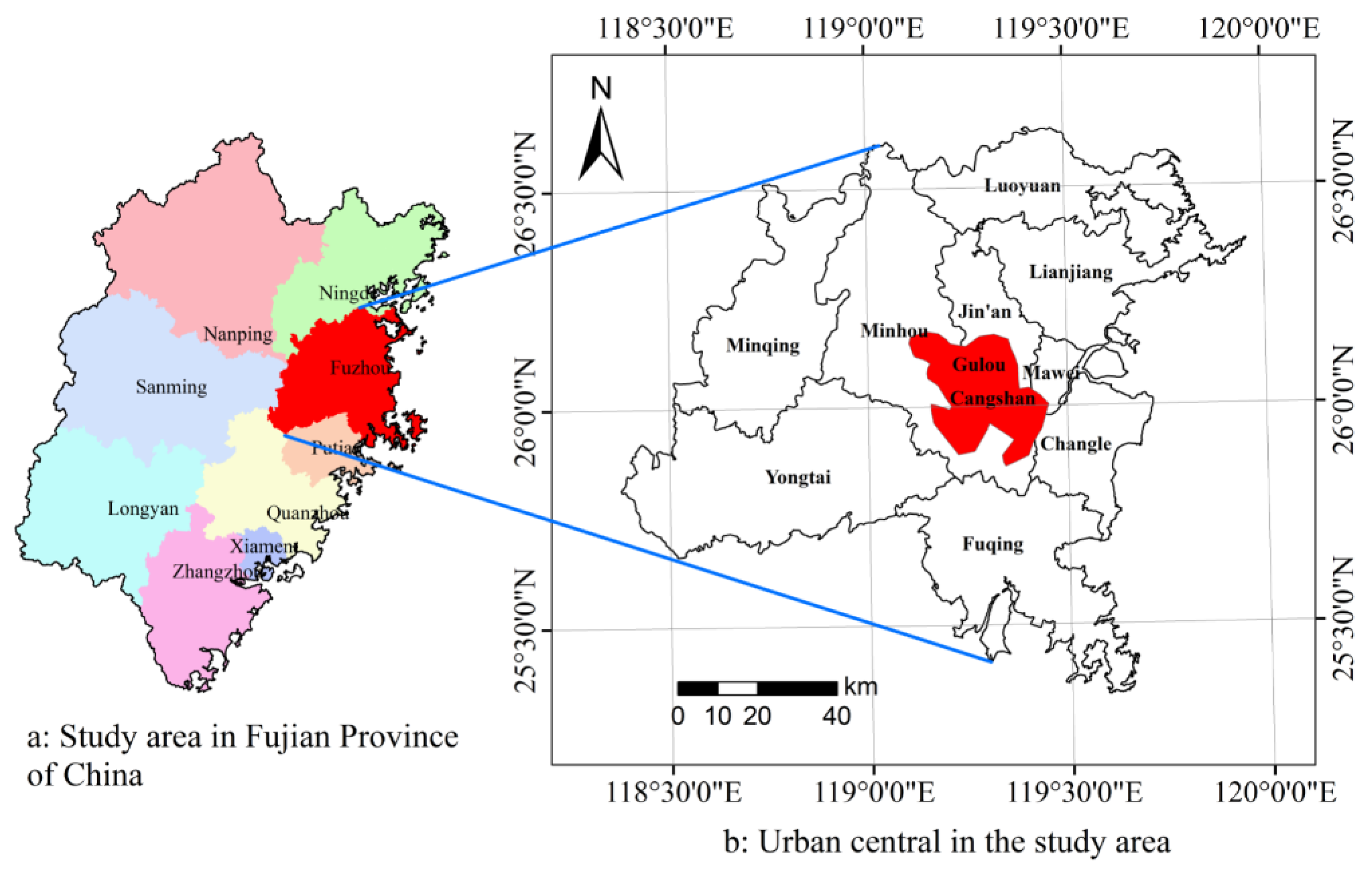
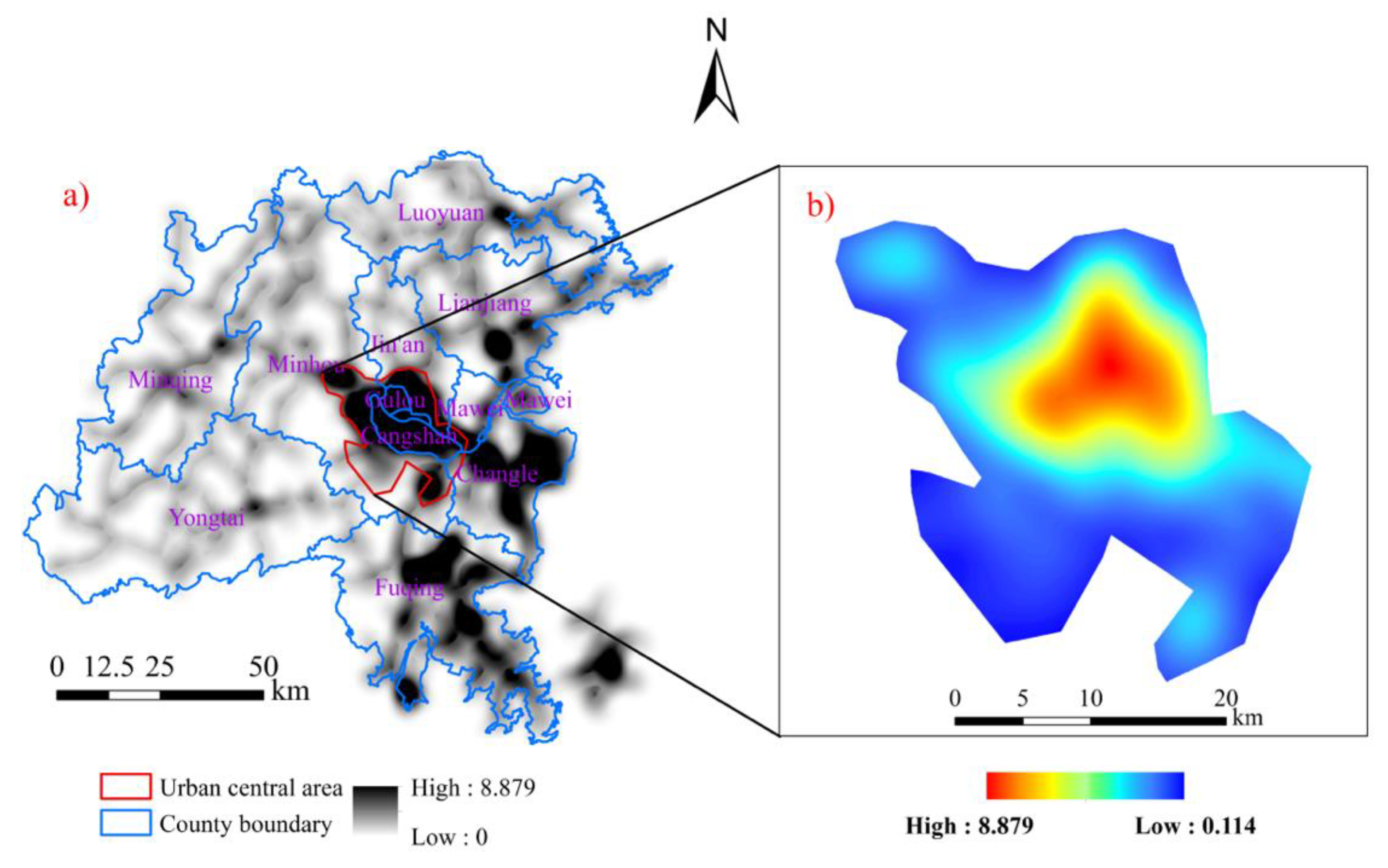
2.1. Study Area

Fuzhou (25°157′~26°39′N, 118°08′~120°31′E) is the capital of Fujian Province, which is a developed prefecture-level city located on the west coast of the Taiwan Strait in the lower reaches of the Minjiang River (Figure 1). Fuzhou governs six districts and seven counties, consisting of 147 towns and covering a total area of more than 12,153 km². This area belongs to the subtropical monsoon climate zone, with an average annual temperature of 20.75 ℃ and an average annual precipitation of 1,359 mm. The precipitation is concentrated in the flood seasons (i.e., May and June). The altitude is between 1 and 802.4 m, with an average of 84 m. According to the latest census (2010), the population was 7,115,370 inhabitants. At the end of 2018, the urbanization rate of the study area was 70.30% [48]. The Integrated City Index of Fuzhou City was ranked 20th in China in 2016, as indicated by the National Development and Reform Commission [49]. Therefore, Fuzhou City is a good case area to explore the spatio–temporal patterns of a road network, which may help contextualize other rapidly growing cities in the country.

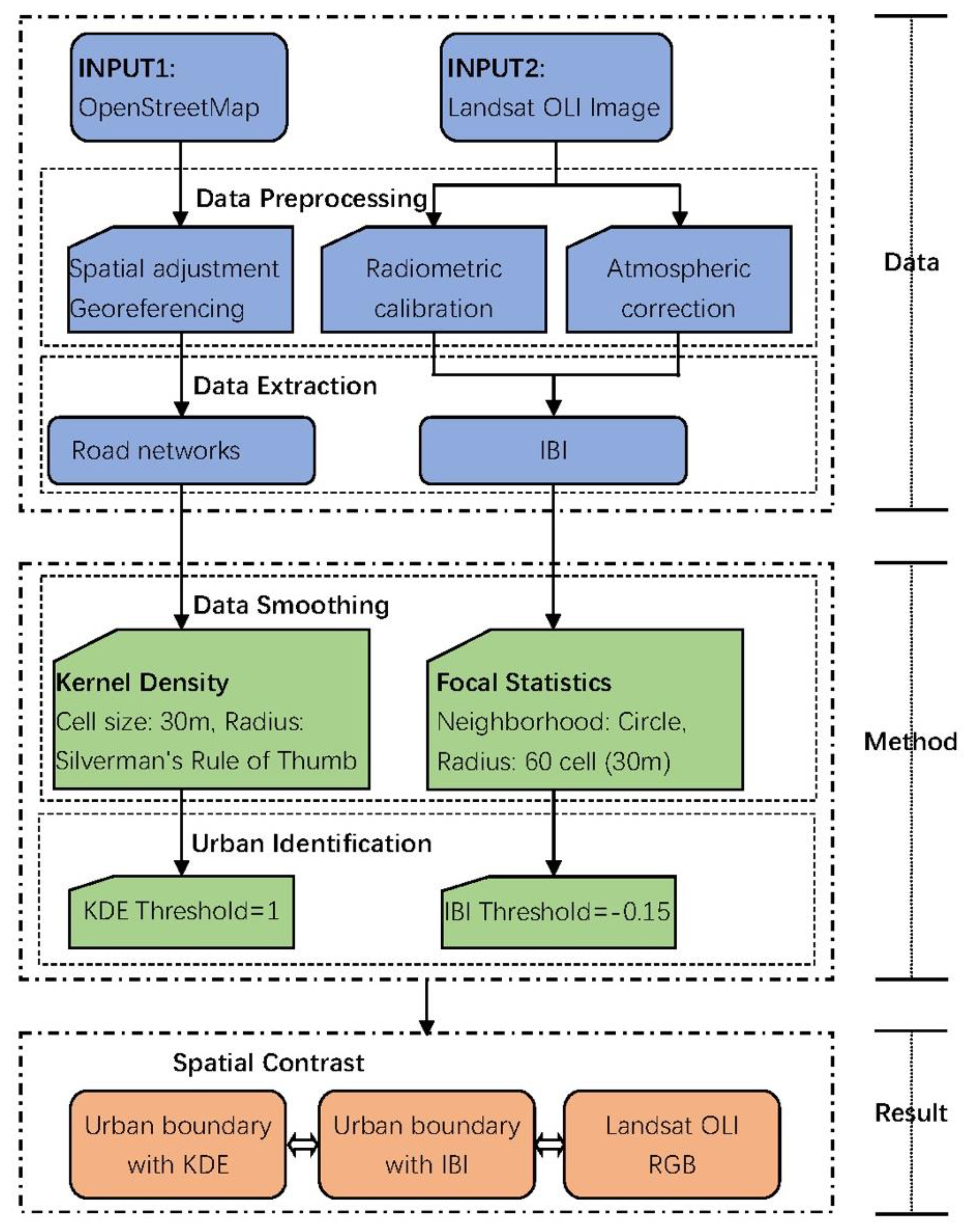
2.2. Identification of Urban Boundary

The framework of this study uses road networks as a data source to delimit the boundaries of urban areas (Figure 2). Firstly, the road network vector data were spatially adjusted and clipped using the administrative division vector maps as a reference. Secondly, KDE was calculated using ArcGIS 10.0 software (Environmental Systems Research Institute, Redlands, California, USA). Thirdly, the optimal threshold of the KDE was set as the basis of a series of spatial analyses of the data, and the boundaries of the urban areas were determined. Fourthly, another dataset (Landsat OLI images) was pre-processed, and the index-based built-up index (IBI) was then extracted. Finally, comparisons between the boundaries delimited by KDE and those by IBI and RGB were conducted to determine the effectiveness of boundary identification using road networks based on KDE.

2.3. Data Sources and Pre-Processing

Firstly, the datasets for the road networks of the study area were obtained from OSM (http://www.geofabrik.de/data/). The road networks were provided as ArcGIS vector datasets containing many attributes (i.e., grade, name, and lanes); however, they also included many duplicate lines, which affected the accuracy of the data. To effectively measure the density of the road network in the study area, we employed the integrated tool in ArcGIS 10.0 software to make the lines coincide if they fell within 100 m. Then, we used the spatial adjustment tool in ArcGIS 10.0 software to perform a spatial transformation of the road network to match the administrative division vector map.

The second dataset was Landsat Operational Land Imager (OLI) (2016-06-25), which was obtained directly from the official website of the US Geological Survey (USGS) (https://glovis.usgs.gov), and used it to extract the built-up area in this study. The pre-processing of the calibration and the conversion to planetary surface reflectance used the guide for the Landsat-8 algorithm posted by USGS using ENVI version 5.1 software [46,50].

2.4. Kernel Density Estimation

KDE was applied to avoid problems related to the arbitrary choice of the grid superimposed onto the road networks [23,29]. The outcome of KDE is affected greatly by the bandwidth of the kernel function. In this study, we used Silverman’s rule of thumb to choose the optimized bandwidth in the ArcGIS 10.0 program, which was generated automatically as the minimum width or length of the studied area divided by 250 [11]. Figure 3 provides visualization maps of the KDE for the road network.

2.5. Index-Based Built-Up Index

The NDBI and the IBI have been widely employed to extract urban built-up areas. A previous study indicated that the NDBI may be mixed with vegetation noise and must be further filtered by the normalized difference vegetation index (NDVI) to obtain more objective results [40], while the IBI can achieve overall higher accuracy than the NDBI [51]. For this reason, IBI was applied to delineate the urban built-up areas of the study area. The formula for IBI is expressed as follows:

IBI={2B_SWI1/(B_SWI1+B_NIR)-[B_NIR/(B_NIR+B_Red)+B_Green/(B_Green+B_SWI1)]}/{2B_SWI1/(B_SWI1+B_NIR)
+[B_NIR/(B_NIR+B_Red)+B_Blue/(B_Blue+B_SWI1)}

(1)

where B_i is the planetary reflectance value of each band in the OLI sensors.

Next, a neighborhood technique (i.e., a focal statistics tool) was employed to smooth the distribution of the IBI using ArcGIS 10.0. Focal statistics are defined as the estimated value of each grid using an average value within a certain circle. Therefore, the estimated value is affected by the radius of the circle. In this analysis, the default radius was set as three cells.

2.6. Geographical Variation Analysis

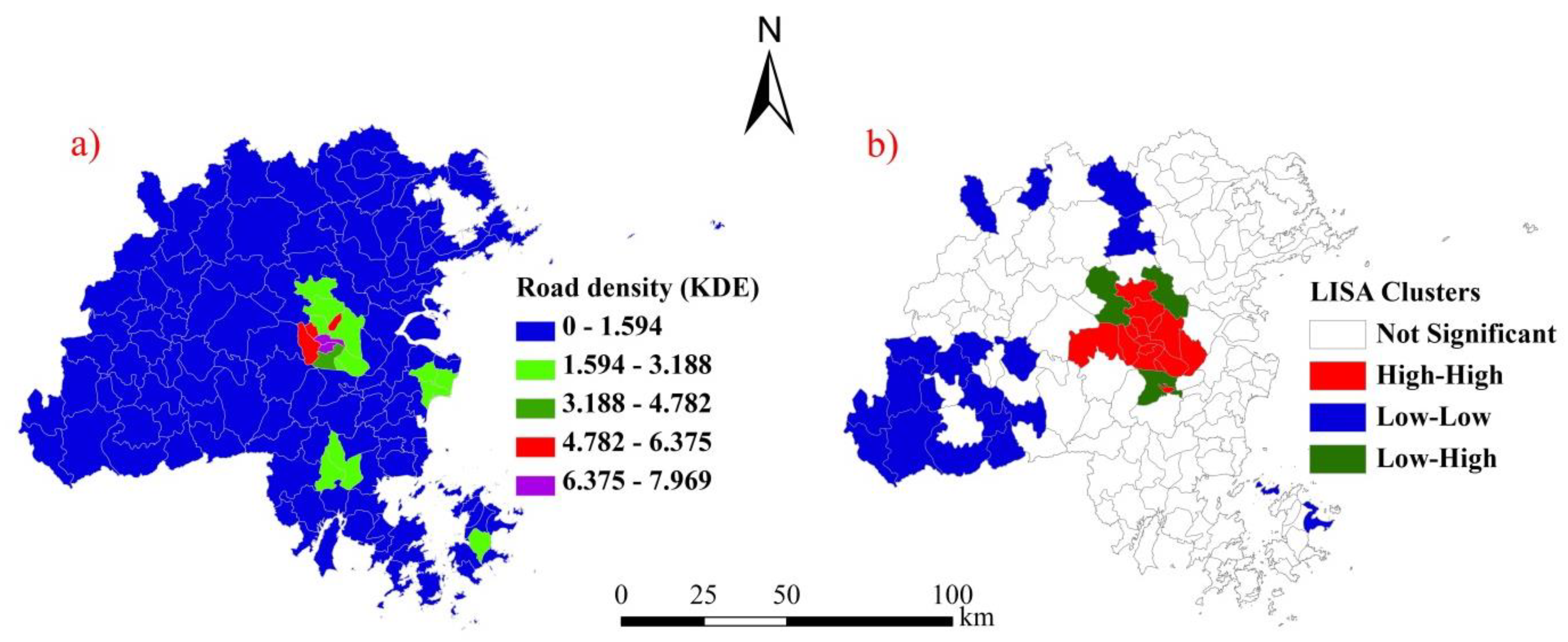
2.6.1. Spatial Autocorrelation Analysis

The spatial autocorrelation of the KDE for the study area was observed using the ESDA technique [52]. Both the global spatial autocorrelation (i.e., global Moran’s I) and the local spatial autocorrelation (i.e., the local indicator of spatial association (LISA)) were calculated using the ArcGIS 10.0 program in this study. When executing the program, the method of inverse distance weighting was selected to conceptualize the spatial relationships between neighbors, and the default neighborhood sizes were adopted [53,54]. The reason for choosing inverse distance weighting is based on the first law of geography [55], which mandates that “everything is related to everything else, but near things are more related than distant things”. A spatial paradigm map, consisting of five categories of clusters, was then created: “high–high” (hot spots, where the density level of the observation itself and that of the surrounding area is high, and the spatial difference between the two observations is relatively small); “low–low” (cold spots, where the density level of the observation itself and the surrounding area are low, and the spatial difference between the two observations is relatively small); “low–high” (the density level of the observation itself is low, while that of the surrounding areas is high, and there is a large spatial difference between the two neighbors); “high–low” (the density level of the observation itself is high, while that of the surrounding areas is low, and there is a large spatial difference between the two neighbors); and “not significant” (Figure 4b).

2.6.2. Semivariance Analysis

Semivariance analysis, a commonly used method for geostatistics, was then used to measure the spatial variation of the neighboring observations. Generally, the value of the semivariance function increases with an increase in the sample point distance and rises to a basically stable constant (i.e., the sill) at a certain interval (i.e., the range). Therefore, the semivariance function is usually characterized by the following parameters [53]: the sill (C₀+C), range (A₀), nugget effect (C₀), spatially dependent structural variance (C), and ratio of the nugget effect (C₀) to the sill (C₀+C) [53]. In this study, a semi-variogram was calculated using the SAM v. 3.1 program. The coefficient of determination (r²) and residual sum of squares (RSS) were used to screen the optimal semivariance functions including linear, sphericity, and exponential functions, as well as Gaussian models [56].

2.7. Sampling Strategies

To explore the scale dependence of the road network distribution, different grain sizes (30, 60, 90, 150, 300, 600, 900, 1,200, 1,500, and 1,800 m) were set as the sample units in the semi-variogram analysis.

3. Results and Discussion

3.1. Spatial Patterns of the Road Density at Different Levels

Figure 3 illustrates the spatial distribution of the road networks (i.e., the KDE) at a 30 m grid level for the study area. This figure shows that the urban central area, including the districts of Gulou, Cangshan, Taijian, and Changle, had the highest density of road networks; the central area of each county, including Luoyuan, Lianjiang, Fuqing, and Minqing, had moderately dense road networks, while the other areas, such as county, village, and mountainous areas, had the lowest density of road networks (Figure 3a). Simultaneously, for the urban central area, the density of road networks decreased gradually from the center to the periphery in the urban central area (Figure 3b).

Figure 4 illustrates the spatial distribution of the KDE at the town level for the study area, with all the towns divided into five equidistant categories according to the density of their road networks. This also shows that the urban central area had the highest density of road networks, while most of the other areas belonged to the lowest class of the KDE (Figure 4a). The results of the spatial autocorrelation analysis revealed some notable characteristics, including the hot spots (i.e., the high–high cluster), cold spots (i.e., the low–low cluster), and the low–high cluster in the road networks of the study area (Figure 4b).

Comparing the results of the two different grain size scales (i.e., at grid and town levels), we found that there were multiple sub-centers distributed in each county at the finer level (i.e., at a 30 m grain size), as well as a large urban center in the study area (Figure 3), while only three sub-centers and one large urban center were discovered at the coarse level (i.e., the town level) (Figure 4). This indicates that some useful information may be obscured at the coarse grain size (i.e., the town level). Whether at the 30-m grid level or at the town level, the KDE shows that there was a large gap between the urban and rural areas, with developed road networks in the former, and undeveloped in the latter.

Figure 5 indicates that the spatial variation in the KDE had a strong positive correlation within a range of about 25 km, with a negative correlation beyond a range of 25 km. This range is similar to that of the urban central area (Figure 3), which reveals the differences in the distribution of road networks between urban and rural areas. Thus, the above results may contribute significantly to delimiting the built-up area for the region.

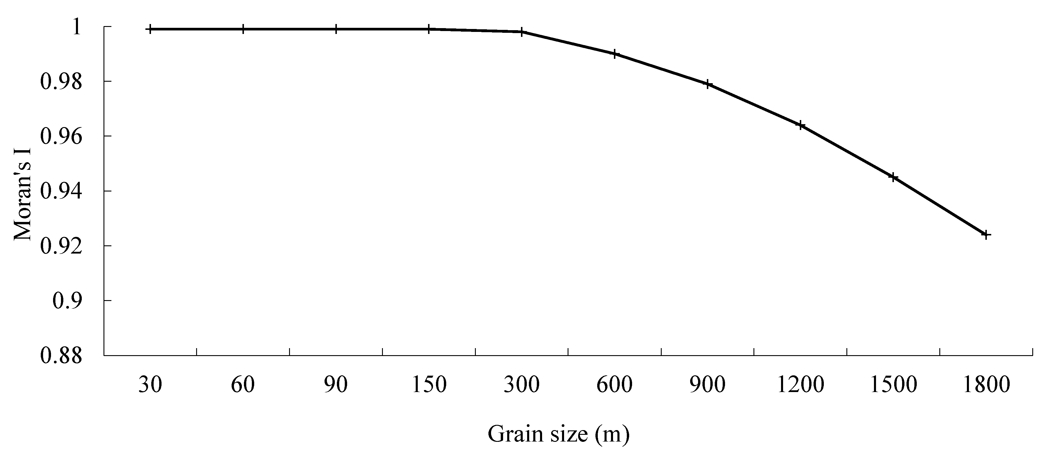
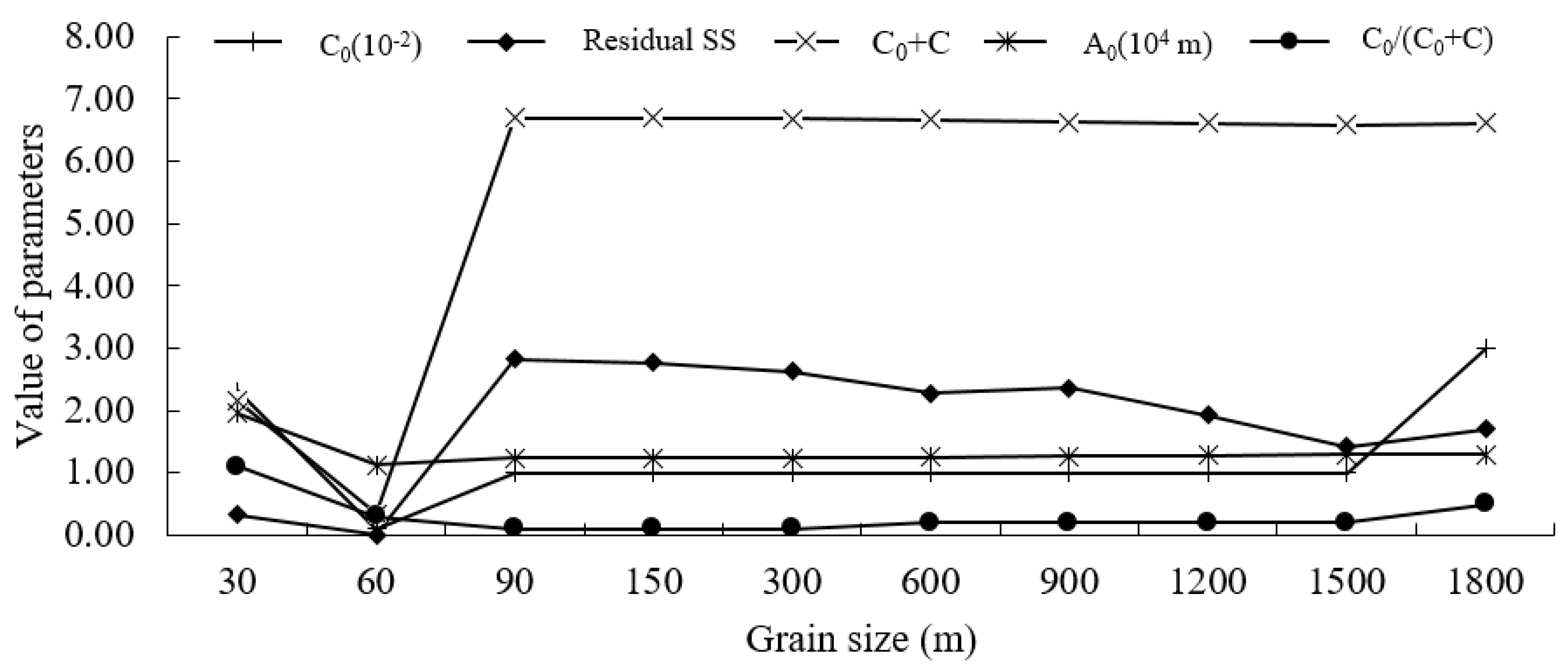
3.2. Scale Effect of Spatial Patterns in Road Density in the Downtown Area

Spatial patterns include both spatial dependence and spatial heterogeneity, with spatial heterogeneity stemming from a variation in spatial dependence [57]. The first law in geography is essentially a principle of spatial autocorrelation [55]. This also implies that spatial variations in a certain geographic attribute of any two locations may occur with an increase in the separate distances. Thus, the second law in geography reveals that spatial heterogeneity is ubiquitous across a wide range of spatial scales [58]. Therefore, to better understand the quantitative characteristics of a road network, the scale effects of spatial patterns in the road distribution must be explored.

Because there was a large gap between the urban and rural areas in terms of KDE, with the urban central area much higher than the rural area, we used the former as a case to further examine the scale effect of spatial patterns in the distribution of road networks. Figure 6 and Figure 7 show that the parameters of global spatial autocorrelation and semivariograms for the road networks change with grain size. It is clear that the parameters of spatial heterogeneity were not uniform across the landscape under different grain sizes. The values of C₀, (C₀+C), A₀, and residual SS showed a similar trend. The initial value (i.e., the 30 × 30 m grain size) was relatively high, but decreased to a low at 60 m and then increased to a peak at 90 m (Figure 6); however, from 150 m, the parameters of the semivariograms tended to be relatively invariable. Additionally, the values of Moran’s I decreased more significantly from 150 m and then sharply declined from 300 m (Figure 7). If the grain size is too small/large to accurately mirror the spatial heterogeneity of the road density, it cannot accurately describe the relevant spatial heterogeneity and spatial dependence. Based on this analysis, 150 m was determined to be a suitable grain size to weaken the scale effects. Thus, 150 m was employed as the grain size to explore the spatial patterns of the road density distribution.

We extended our research by comparing the effects of different grain sizes on the spatial patterns of KDE. We found that the road networks were better characterized by a fine grain size (150 m) than by a coarse grain size (town level) (Figure 3 and Figure 4). This is because the artificial definition of analysis units can affect the statistical results, which has been defined as the modifiable areal unit problem (MAUP) in the geographical literature [59]. One of the most widespread tools to detect the MAUP is a semivariogram. This supports our use of a semivariogram for analyzing spatial heterogeneity in the distribution of the KDE, which will be discussed further in the following section.

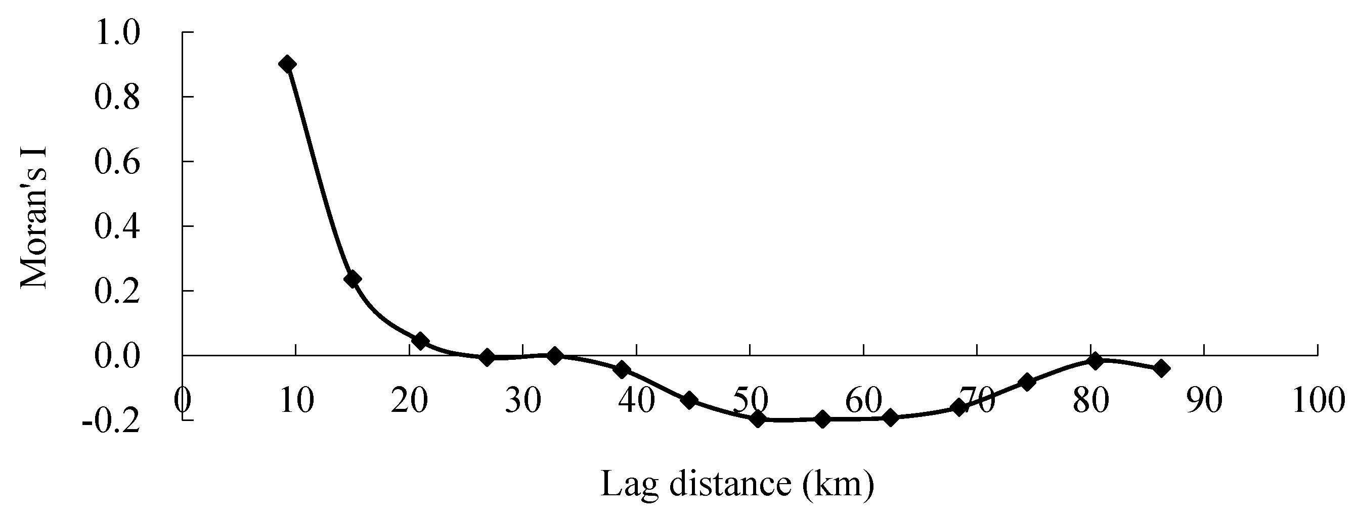
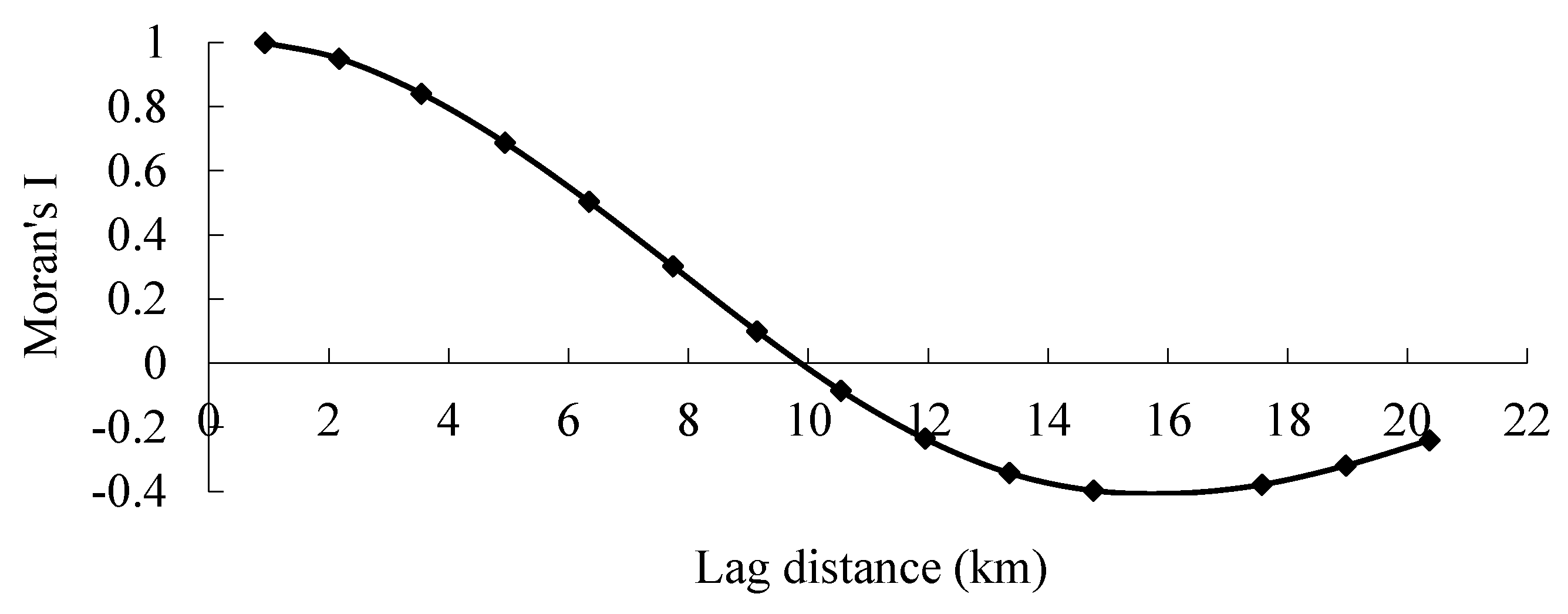
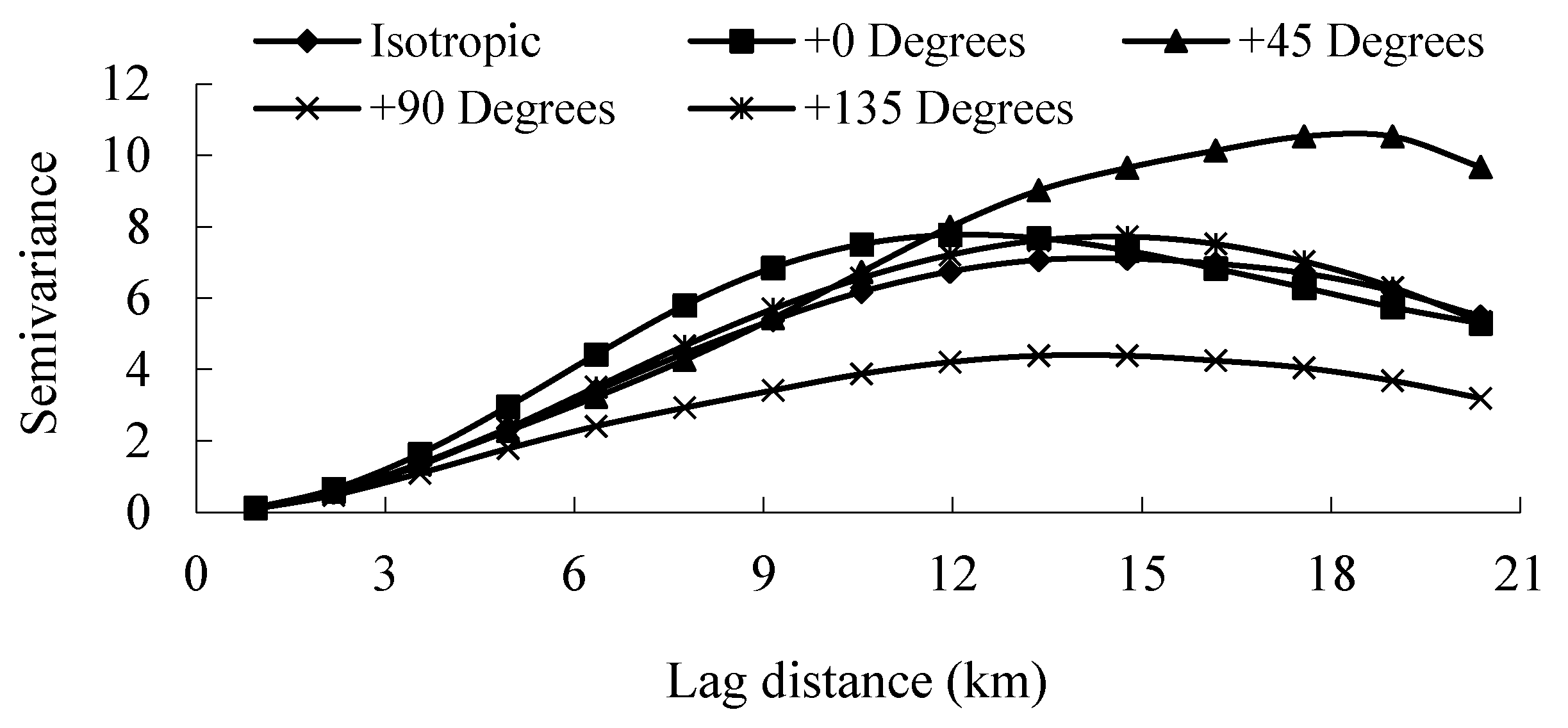
3.3. Characteristics of Spatial Heterogeneity in the Road Density in the Downtown Area

The Moran’s I of the KDE is shown at different spatial scales in Figure 8. Overall, the curve showed a downward trend, indicating that the spatial heterogeneity in the KDE increased with an increase in lag distance. The spatial associations of the KDE between each pair of locations were positive within a range of 10 km and changed to a negative beyond a 10-km distance. This distribution is in line with another geographical attribute, the remote sensing ecological index, which was found to have the same spatial associations [60]. This suggests to some extent that the geographical characteristics of the urbanization process are obvious. Moreover, our analysis of local spatial autocorrelation also showed that the KDE has obvious hot spots (i.e., high–high clusters) in the urban central areas and cold spots (i.e., low–low clusters) in the western section of the study area (Figure 4b). Thus, by using the description and visualization of spatial statistics, the ESDA employed here can explore spatial dependence and spatial heterogeneity and reveal the spatial paradigm mechanism of road network distribution. More importantly, these features of the map highlight the urban and rural differences in the construction of infrastructure as a result of the observable urban boundary.

SA provides another way to visualize the spatial autocorrelation for observations, which accounts for a threshold distance at which spatial dependence exists and beyond which spatial heterogeneity exists [53].

Table 1. Parameters of the spatial heterogeneity of KDE in 2016 (150 m grain size).

	Isotropic	Anisotropic
Model	Gaussian	Exponential
		0	45	90	135
C0	0.010	0.010
C	6.683	10.449
C0+C	6.693	10.549
A0	12384	11440–18660
C0/(C0+C)	0.001	0.001
Dimension (D)	1.365	1.400	1.282	1.440	1.344
R2	0.968	0.849	0.976	0.885	0.905
Residual Sum of Squares (RSS)	2.770	-

describes the parameters of the SA for both the isotropic variogram and the anisotropic variogram for the KDE. The Gaussian (isotropic) and exponential (anisotropic) models best satisfy the hypothesis, considering the values of R² and RSS.

According to the parameters, the values of C₀ for both the isotropic variogram and the anisotropic variogram were relatively small (0.010), indicating that the measurement error (including the sampling error) was small. As a result, the outcomes could be employed to analyze the spatial paradigm in the KDE for the study area. The high values of C (6.683 and 10.449), the low values of C₀/(C + C₀) (0.001), and the values of the fraction dimension index (D) distance from 2 for both the isotropic and the anisotropic variogram all indicate that the spatial paradigm structure of the road networks is the critical factor for spatial dependence in the distribution of road density itself.

Further, the isotropic model also suggests that the observations were fully independent when the distance between the observations exceeded 12,384 m (Table 1). This distance is identical to the urban core area (i.e., the brightly colored clusters in Figure 3b), which is the center of administration, business, and finance in the region and has a higher density of road networks than other surrounding areas.

The anisotropy analysis indicated a significant directional effect in the distribution patterns of road networks (Table 1 and Figure 9). For example, the variation ranged from 11.440 to 18.660 km across different directions (Table 1), with a range of about 11 km for most of the directions (i.e., isotropic, 0°, 90°, and 135°) and approximately 19 km for the 45° direction. Additionally, the values of D were different among all the directions, with the lowest value in the northeast–southwest direction followed by the southeast–northwest direction, indicating that the spatial variations of road networks in these two directions were greater than those of the other two directions. Figure 3b shows that the northeast–southwest (i.e., 45° direction) length of the core area was around 19 km.

The cause of the intense effect of anisotropy is possibly due to the orientation in the spatial structure of the road network itself alongside topography and its economy, as well as urbanization and development processes. In the past two decades, the urban central area has been expanding along the southeasterly direction and the Minjiang River (http://english.jxfz.gov.cn/About_Fuzhou/), leading to the shape of the urban central area being wider in the northeast–southwest and southeast–northwest directions (Figure 3b). In these two directions, the space is covered by a gradual or abrupt change between the urban core area and urban–rural fringe, so the road density changes more greatly than that in the other directions. This confirms that it is both necessary and effective to use KDE and SA to explore the spatial structural characteristics of road networks.

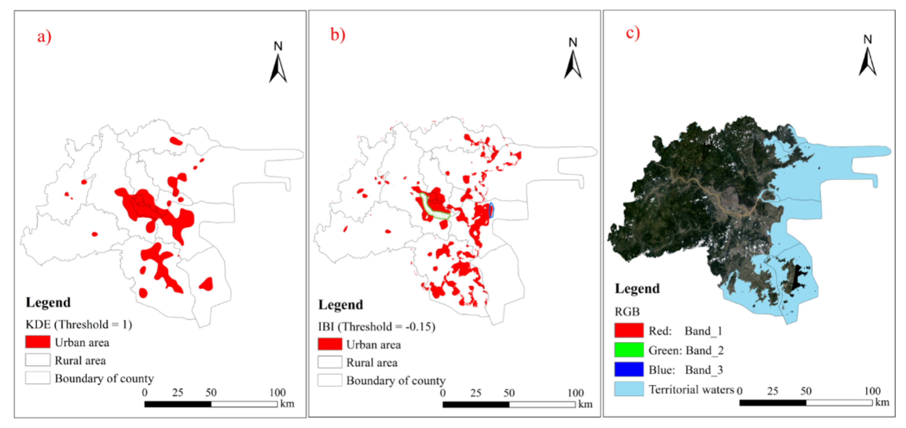
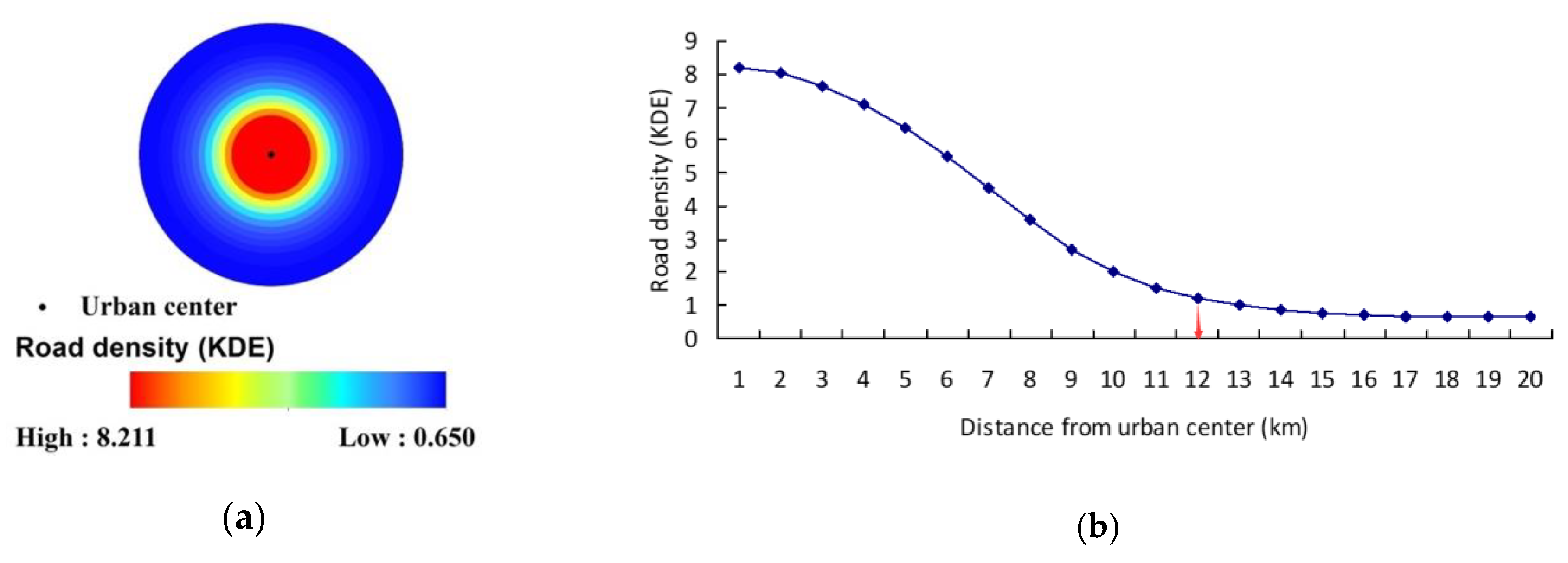
3.4. Delimitation of the Urban Boundary

At the regional level, the outcome of our KDE analysis verifies the previous conclusions, which highlight the density peaks of the road networks in the central city [27]. We also found that the urban area possessed much denser road networks than non-urban areas (i.e., rural areas) (Figure 3 and Figure 4). The urban–rural gradient analysis of the KDE is further characterized by the obvious “density island effect” of road networks, with a turning point (e.g., 12 km) beyond which the KDE value stabilized at around 1 (Figure 10). This finding matches not only the above-SA result [61], but also the central-place theory, demonstrating that transport infrastructures are more frequently distributed in higher-order places (i.e., towns), but fewer are located in lower-order places (i.e., suburban or rural areas) [45]. Therefore, we confirmed the previous outcomes [27] indicating that the road network was an effective proxy for the structural information of the region that can also be used to segment urban areas [14].

In this study, we further compared the results of the delimitation of an urban area by KDE and IBI extracted from Landsat OLI (Figure 11). According to the turning point (i.e., KDE=1) in Figure 10b, we determined a KDE threshold = 1 to identify the urban boundary here. In terms of the threshold of the IBI, a value of -0.15 was set to determine the boundary after a careful comparison with the Landsat RGB image through visual interpretation.

Figure 11 illustrates the urban areas segmented by KDE, IBI, and the RGB images of Landsat OLI. Our outcomes are in line with those of previous studies [17,47], revealing that the density distribution of the road networks is very close to that of the IBI. Moreover, the spatial distribution of the urban areas segmented using KDE better matched the urban boundaries than the spatial distribution of IBI compared to the RGB image (Figure 11). Our research corroborates previous findings [14,17,47], suggesting that a measurement of KDE may supply additional structural information for the delimitation of urban areas. This reveals that our method of quickly identifying urban boundaries is effective.

Notably, the boundaries obtained by the KDE were better than those of the IBI. The urban land acquired by the latter was discrete but not continuous, even when we employed focal statistics to smooth the distribution of the IBI. This is because there were different land cover types within the urban area, including vegetation, bare land, and a water area. The IBI could only enhance building land information, while the other land covers could not be extracted. This is why we used focal statistics to smooth the distribution of the IBI, as it is very challenging to assign bandwidth (i.e., the radius) and a radius that is too large will cause the overestimation of urban boundaries. Otherwise, the urban area was not continuous, as in the result of Figure 11b. For example, the large strip of river and open green space on both sides (i.e., the green cluster in Figure 11b) was not covered in the urban area because the width of the gap was too large (even the smoothing method could not make up for this gap). This was also true for some white holes (i.e., large green spaces) in the red plaque. Additionally, the resulting urban built-up map could not remove the noise of the barren areas in the suburbs or the muddy estuaries (i.e., the blue cluster in Figure 11b), which could lead to an inflated urban border. In addition, the red patches were dispersed across the study area. All these results reveal, to some extent, that there are some limitations in determining urban boundaries using IBI. Therefore, further artificial intelligence methods (such as cellular automata) or extra manual delineation are needed if urban boundaries are to be demarcated by the density of built-land.

Nonetheless, our proposed KDE method for identifying urban areas is simple, and its results were in line with the observations (Figure 11a). The largest red patch in the middle of the map is the urban center, and the other smaller red patches indicate the central towns of each county in the study area. In the urban central area, the boundary outlined assumes an irregular shape with a width of approximately 25 km, which is very close to the range of variance of Moran’s analysis at the regional level. Therefore, as a proxy, a road network using KDE was used as an active indicator for the delimitation of urban areas.

4. Conclusions

The contributions of the paper are both qualitative and quantitative. Qualitatively, our results offer a good understanding of the spatial distributions of road networks and their effects on the delimitation of urban boundaries. These results show that there is spatial unevenness in the distribution of road networks, both at the regional level and at the downtown level. At the regional level, there is serious polarization in road distribution, with the distribution of road networks being much higher in urban areas than in rural areas. At the downtown level, road density gradually decreases from the center to the periphery.

Quantitatively, the characteristics of spatial heterogeneity derived from ESDA and SA show that (1) a grain size of 150 m was suitable in this case to weaken the scale effects of road distribution; (2) the spatial dependence ranges of the road networks were approximately 25 km for the entire study region and 12 km for the downtown area. Additionally, the spatial variations varied between different directions, with variations of the road networks in the northeast–southwest and southeast–northwest directions being greater than those in the other two directions, which is in line with the urbanization and development processes of the study area. Therefore, our case sheds new light on the application of ESDA and SA to quantify spatial variation in road networks.

Both the qualitative and quantitative results show that the distribution of road networks has a clear urban–rural dual structure, which indicates that road networks can be used as an active tool to identify urban areas for the region. Thus, we proposed a quick and easy way to delimit urban areas using KDE for linear road networks based on Silverman’s rule of thumb to optimize the kernel’s bandwidth. The results also indicate that our proposed method is effective and feasible. Our proposed method can help to overcome the two types of noises caused by treating bare land as built-up land and green built-up areas as forests and crops in image classification using remote sensing datasets in urban–rural fringe zones. Our research suggests that a combination of road density from OSM and spectral information from aerial images may provide more accurate information for urban planning and management to identify urban boundaries at different spatial sizes, from small cities to large metropolises. Our method has the potential to quickly extract urban boundaries for other regions due to the popularity of OSM data. However, there are several limitations that should be noted when adopting our proposed method. Firstly, datasets of road networks from OSM may include many duplicate lines, so the road network needs to be pre-processed, including spatial correction and integration of duplicate lines. Secondly, different bandwidths produce different density patterns, which require changing the kernel’s bandwidth and choosing an appropriate bandwidth to achieve the desired effect for different sizes of cities. Finally, the spatial structures of complete road networks do not change considerably in the short term, so the derived urban area is limited to an existing road network. Therefore, we recommend using KDE for road networks with spectral data to obtain more accurate urban boundaries.

References

1. Mcdonald, R.I.; Green, P.; Balk, D.; Fekete, B.M.; Revenga, C.; Todd, M.; Montgomery, M. Urban growth, climate change, and freshwater availability. Proc. Natl. Acad. Sci. USA 2011, 108, 6312–6317. [Google Scholar] [CrossRef] [PubMed] [Green Version]
2. Gong, P.; Li, X.; Zhang, W. 40-Year (1978–2017) human settlement changes in China reflected by impervious surfaces from satellite remote sensing. Sci. Bull. 2019, 64, 756–763. [Google Scholar] [CrossRef] [Green Version]
3. Heintzman, L.J.; McIntyre, N.E. Quantifying the effects of projected urban growth on connectivity among wetlands in the Great Plains (USA). Landsc. Urban Plan. 2019, 186, 1–12. [Google Scholar] [CrossRef]
4. Liu, X.; Hu, G.; Chen, Y.; Li, X.; Xu, X.; Li, S.; Pei, F.; Wang, S. High-resolution multi-temporal mapping of global urban land using Landsat images based on the Google Earth Engine Platform. Remote Sens. Environ. 2018, 209, 227–239. [Google Scholar] [CrossRef]
5. Barnosky, A.D.; Hadly, E.A.; Bascompte, J.; Berlow, E.L.; Brown, J.H.; Fortelius, M.; Getz, W.M.; Harte, J.; Hastings, A.; Marquet, P.A.; et al. Approaching a state shift in Earth’s biosphere. Nature 2012, 486, 52–58. [Google Scholar] [CrossRef]
6. Schmidt, C.; Domaratzki, M.; Kinnunen, R.P.; Bowman, J.; Garroway, C.J. Continent-wide effects of urbanization on bird and mammal genetic diversity. Proc. R. Soc. B 2020, 287, 20192497. [Google Scholar] [CrossRef]
7. Shi, Y.; Ren, C.; Lau, K.K.; Ng, E. Investigating the influence of urban land use and landscape pattern on PM2.5 spatial variation using mobile monitoring and wudapt. Landsc. Urban Plan. 2019, 189, 15–26. [Google Scholar] [CrossRef]
8. Ramalho, C.E.; Hobbs, R.J. Time for a change: Dynamic urban ecology. Trends Ecol. Evol. 2012, 27, 179–188. [Google Scholar] [CrossRef]
9. Turner, B.L.; Lambin, E.F.; Anette, R. The emergence of land change science for global environmental change and sustainability. Proc. Natl. Acad. Sci. USA 2007, 104, 20666–20671. [Google Scholar] [CrossRef] [Green Version]
10. Forman, R.T.T. Road ecology: A solution for the giant embracing us. Landsc. Ecol. 1998, 13, III–V. [Google Scholar] [CrossRef]
11. Wei, W.; Shi, P.J.; Zhou, J.J.; Xie, B.B. The Road Network Density and Spatial Dependence Analysis Based on Basin Scale—A Case Study on Shiyang River Basin. Appl. Mech. Mater. 2014, 505, 750–754. [Google Scholar] [CrossRef]
12. Barthelemy, M. Spatial Networks. Phys. Rep. 2010, 499, 1–101. [Google Scholar] [CrossRef] [Green Version]
13. Lämmer, S.; Gehlsen, B.; Helbing, D. Scaling laws in the spatial structure of urban road networks. Phys. Stat. Mech. Appl. 2006, 363, 89–95. [Google Scholar] [CrossRef] [Green Version]
14. Borruso, G. Network Density and the Delimitation of Urban Areas. Trans. GIS 2010, 7, 177–191. [Google Scholar] [CrossRef]
15. Su, Q. The effect of population density, road network density, and congestion on household gasoline consumption in U.S. urban areas. Energy Econ. 2011, 33, 445–452. [Google Scholar] [CrossRef]
16. Quinn, P. Road density as a proxy for population density in regional-scale risk modeling. Nat. Hazards J. Int. Soc. Prev. Mitig. Nat. Hazards 2013, 65, 1227–1248. [Google Scholar] [CrossRef]
17. Zhang, Q.; Wang, J.; Peng, X.; Gong, P.; Shi, P. Urban built-up land change detection with road density and spectral information from multi-temporal Landsat TM data. Int. J. Remote Sens. 2002, 23, 3057–3078. [Google Scholar] [CrossRef]
18. Strano, E.; Nicosia, V.; Latora, V.; Porta, S.; Barthélemy, M. Elementary processes governing the evolution of road networks. Sci. Rep. UK 2012, 2, 296. [Google Scholar] [CrossRef] [Green Version]
19. Hu, X.; Zhang, L.; Ye, L.; Lin, Y.; Qiu, R. Locating spatial variation in the association between road network and forest biomass carbon accumulation. Ecol. Indic. 2017, 73, 214–223. [Google Scholar] [CrossRef]
20. Garrison, W.L. Connectivity of the Interstate Highway System. Pap. Reg. Sci. 2010, 6, 121–137. [Google Scholar] [CrossRef]
21. Barabási, A.L.; Bonabeau, E. Scale-free networks. Sci. Am. 2003, 288, 60. [Google Scholar] [CrossRef] [PubMed]
22. Hu, X.S.; Wu, C.Z.; Wang, J.K.; Qiu, R.Z. Identification of spatial variation in road network and its driving patterns: Economy and population. Reg. Sci. Urban Econ. 2018, 71, 37–45. [Google Scholar] [CrossRef]
23. Cai, X.; Wu, Z.; Cheng, J. Using kernel density estimation to assess the spatial pattern of road density and its impact on landscape fragmentation. Int. J. Geogr. Inf. Sci. 2013, 27, 222–230. [Google Scholar] [CrossRef]
24. Mo, W.; Wang, Y.; Zhang, Y.; Zhuang, D. Impacts of road network expansion on landscape ecological risk in a megacity, China: A case study of Beijing. Sci. Total Environ. 2017, 574, 1000–1011. [Google Scholar] [CrossRef] [PubMed] [Green Version]
25. Lin, Y.; Hu, X.; Zheng, X.; Hou, X.; Zhang, Z.; Zhou, X.; Qiu, R.; Lin, J. Spatial variations in the relationships between road network and landscape ecological risks in the highest forest coverage region of China. Ecol. Indic. 2019, 96, 392–403. [Google Scholar] [CrossRef]
26. Hawbaker, T.J.; Radeloff, V.C.; Hammer, R.B.; Clayton, M.K. Road Density and Landscape Pattern in Relation to Housing Density, and Ownership, Land Cover, and Soils. Landsc. Ecol. 2005, 20, 609–625. [Google Scholar] [CrossRef]
27. Zhang, Z.; Tan, S.; Tang, W. A GIS-based Spatial Analysis of Housing Price and Road Density in Proximity to Urban Lakes in Wuhan City, China. Chin. Geogr. Sci. 2015, 25, 775–790. [Google Scholar] [CrossRef] [Green Version]
28. Miller, J.R.; Joyce, L.A.; Knight, R.L.; King, R.M. Forest roads and landscape structure in the southern Rocky Mountains. Landsc. Ecol. 1996, 11, 115–127. [Google Scholar] [CrossRef]
29. Gatrell, A.C.; Bailey, T.C.; Diggle, P.J.; Rowlingson, B.S. Spatial Point Pattern Analysis and Its Application in Geographical Epidemiology. Trans. Inst. Br. Geogr. 1996, 21, 256–274. [Google Scholar] [CrossRef]
30. Coffin, A.W. From roadkill to road ecology: A review of the ecological effects of roads. J. Transp. Geogr. 2007, 15, 396–406. [Google Scholar] [CrossRef]
31. Li, T.; Li, W.; Qian, Z. Variations in ecosystem service value in response to land use changes in Shenzhen. Ecol. Econ. 2010, 69, 1427–1435. [Google Scholar]
32. Qiu, G.Y.; Zou, Z.D.; Li, X.Z.; Li, H.Y.; Guo, Q.P.; Yan, C.H.; Tan, S.L. Experimental studies on the effects of green space and evapotranspiration on urban heat island in a subtropical megacity in China. Habitat Int. 2017, 68, 30–42. [Google Scholar] [CrossRef]
33. Peng, J.; Lin, H.; Chen, Y.; Blaschke, T.; Luo, L.; Xu, Z.; Hu, Y.; Zhao, M.; Wu, J. Spatiotemporal evolution of urban agglomerations in China during 2000–2012: A nighttime light approach. Landsc. Ecol. 2020, 35, 421–434. [Google Scholar] [CrossRef]
34. Zhou, W.Q.; Huang, G.L.; Pickett, S.T.A.; Cadenasso, M.L. 90 years of forest cover change in an urbanizing watershed: Spatial and temporal dynamics. Landsc. Ecol. 2011, 26, 645–659. [Google Scholar] [CrossRef]
35. Kuang, W.H.; Liu, J.Y.; Dong, J.W.; Chi, W.F.; Zhang, C. The rapid and massive urban and industrial land expansions in China between 1990 and 2010: A CLUD-based analysis of their trajectories, patterns, and drivers. Landsc. Urban Plan. 2016, 145, 21–33. [Google Scholar] [CrossRef]
36. Fenta, A.A.; Yasuda, H.; Haregeweyn, N.; Belay, A.S.; Hadush, Z.; Gebremedhin, M.A.; Mekonnen, G. The dynamics of urban expansion and land use/land cover changes using remote sensing and spatial metrics: The case of Mekelle City of northern Ethiopia. Int. J. Remote Sens. 2017, 38, 4107–4129. [Google Scholar] [CrossRef]
37. Liu, Y.Q.; Song, W.; Deng, X.Z. Understanding the spatiotemporal variation of urban land expansion in oasis cities by integrating remote sensing and multi-dimensional DPSIR-based indicators. Ecol. Indic. 2019, 96, 23–37. [Google Scholar] [CrossRef]
38. Xu, H.; Huang, S.; Zhang, T. Built-up land mapping capabilities of the ASTER and Landsat ETM+ sensors in coastal areas of southeastern China. Adv. Space Res. 2013, 52, 1437–1449. [Google Scholar] [CrossRef]
39. Xian, G.; Crane, M.; McMahon, C. Quantifying multi-temporal urban development characteristics in Las Vegas from Landsat and ASTER data. Photogramm. Eng. Remote Sens. 2008, 74, 473–481. [Google Scholar] [CrossRef]
40. Zha, Y.; Gao, J.; Ni, S. Use of normalized difference built-up index in automatically mapping urban areas from TM imagery. Int. J. Remote Sens. 2003, 24, 583–594. [Google Scholar] [CrossRef]
41. Xu, Y.Y.; Xie, Z.; Wu, L.; Chen, Z.L. Multilane roads extracted from the OpenStreetMap urban road network using random forests. Trans. GIS 2019, 23, 224–240. [Google Scholar] [CrossRef]
42. Brovelli, M.A.; Minghini, M.; Molinari, M.; Mooney, P. Towards an Automated Comparison of OpenStreetMap with Authoritative Road Datasets. Trans. GIS 2017, 21, 191–206. [Google Scholar] [CrossRef] [Green Version]
43. Wu, S.B.; Du, C.; Chen, H.; Xu, Y.X.; Guo, N.; Jing, N. Road Extraction from Very High Resolution Images Using Weakly labeled OpenStreetMap Centerline. ISPRS Int. J. Geo-Inf. 2019, 8, 478. [Google Scholar] [CrossRef] [Green Version]
44. Yang, D. Mapping Regional Landscape by Using OpenstreetMap (OSM): A Case Study to Understand Forest Patterns in Maya Zone, Mexico; IGI Global: Hershey, PA, USA, 2019. [Google Scholar]
45. Hong, Y.; Yao, Y. Hierarchical community detection and functional area identification with OSM roads and complex graph theory. Int. J. Geogr. Inf. Sci. 2019, 33, 1569–1587. [Google Scholar] [CrossRef]
46. Xu, H.; Feng, D.; Wen, X. Urban Expansion and Heat Island Dynamics in the Quanzhou Region, China. IEEE J. Select. Top. Appl. Earth Obs. Remote Sens. 2009, 2, 74–79. [Google Scholar] [CrossRef]
47. Wang, J. Application of the linear feature detection system—LINDA to image segmentation from remotely sensed data. Remote Sens. Rev. 2009, 13, 49–66. [Google Scholar] [CrossRef]
48. Airey, T. The impact of road construction on the spatial characteristics of hospital utilization in the Meru district of Kenya. Soc. Sci. Med. 1992, 34, 1135–1146. [Google Scholar] [CrossRef]
49. Ahmad, J.; Malik, A.S.; Xia, L. Effective techniques for vegetation monitoring of transmission lines right-of-ways. In Proceedings of the IEEE International Conference on Imaging Systems and Techniques, Penang, Malaysia, 17–18 May 2011. [Google Scholar]
50. Kilic, A.; Allen, R.; Trezza, R.; Ratcliffe, I.; Kamble, B.; Robison, C.; Ozturk, D. Sensitivity of evapotranspiration retrievals from the METRIC processing algorithm to improved radiometric resolution of Landsat 8 thermal data and to calibration bias in Landsat 7 and 8 surface temperature. Remote Sens. Environ. 2016, 185, 198–209. [Google Scholar] [CrossRef] [Green Version]
51. Essa, W.; Verbeiren, B.; van der Kwast, J.; Van de Voorde, T.; Batelaan, O. Evaluation of the DisTrad thermal sharpening methodology for urban areas. Int. J. Appl. Earth Obs. Geoinfor. 2012, 19, 163–172. [Google Scholar] [CrossRef]
52. Yang, Y.; Wong, K.K.F. Spatial Distribution of Tourist Flows to China’s Cities. Tour. Geogr. 2013, 15, 338–363. [Google Scholar] [CrossRef]
53. Hu, X.; Hong, W.; Qiu, R.; Hong, T.; Chen, C.; Wu, C. Geographic variations of ecosystem service intensity in Fuzhou City, China. Sci. Total Environ. 2015, 512, 215–226. [Google Scholar] [CrossRef] [PubMed]
54. Łukaszyk, S. A new concept of probability metric and its applications in approximation of scattered data sets. Comput. Mech. 2004, 33, 299–304. [Google Scholar] [CrossRef]
55. Tobler, W.R. A computer model simulation of urban growth in the Detroit region. Econ. Geogr. 1970, 46, 234–240. [Google Scholar] [CrossRef]
56. Davis, J.C. Statistics and Data Analysis in Geology, 3rd ed.; John Wiley and Sons: Hoboken, NJ, USA, 1986. [Google Scholar]
57. Wu, J.G. Effects of changing scale on landscape pattern analysis: Scaling relations. Landsc. Ecol. 2004, 19, 125–138. [Google Scholar] [CrossRef]
58. Goodchild, M.F. The fundamental laws of GIScience. In Proceedings of the Paper presented at the Summer Assembly of the University Consortium for Geographic Information Science, Pacific Grove, CA, USA, 3 June 2003. [Google Scholar]
59. He, Z.; Zhao, W.; Chang, X. The modifiable areal unit problem of spatial heterogeneity of plant community in the transitional zone between oasis and desert using semivariance analysis. Landsc. Ecol. 2007, 22, 95–104. [Google Scholar] [CrossRef]
60. Hu, X.S.; Xu, H.Q. A new remote sensing index for assessing the spatial heterogeneity in urban ecological quality: A case from Fuzhou City, China. Ecol. Indic. 2018, 89, 11–21. [Google Scholar] [CrossRef]
61. Hosking, P.L. Network Analysis in Geography. N. Z. Geogr. 2010, 28, 102–103. [Google Scholar] [CrossRef]
Figure 1. Location of the study area.
Ijgi 09 00204 g001
Figure 2. Steps to quickly identify urban boundaries using road networks based on kernel density estimation (KDE). IBI, index-based built-up index; RGB, red, green, and blue; OLI, Operational Land Imager.
Ijgi 09 00204 g002
Figure 3. Kernel density estimation of the road network at a 30 m grid level (km/km2): (a) the entire area; (b) the urban central area.
Ijgi 09 00204 g003
Figure 4. Kernel density estimation (KDE) of the road network at the town level (km/km2): (a) spatial distribution, (b) local indicator of spatial association (LISA) clusters (Moran’s I = 0.801; r2=0.762; p-value=0).
Ijgi 09 00204 g004
Figure 5. Moran’s I of KDE showing responses to the distance across the entire area (at the town level).
Ijgi 09 00204 g005
Figure 6. Parameters of spatial heterogeneity showing responses to grain sizes.
Ijgi 09 00204 g006
Figure 7. Moran’s I of KDE showing responses to grain sizes.
Ijgi 09 00204 g007
Figure 8. Moran’s I of KDE showing responses to distance (150 m grain size).
Ijgi 09 00204 g008
Figure 9. Variance function curve of KDE for all directions (150 m grain size).
Ijgi 09 00204 g009
Figure 10. Urban–rural gradient analysis of the kernel density estimation (KDE) of road networks (km/km2). (a) spatial distribution of KDE in urban-rural gradient, (b) curve chart of KDE in urban-rural gradient. The center of the circle is the center of the urban area of Fuzhou City; the radius represents the distance from the urban center; the larger the radius, the greater the distance (radius varying from 1 to 20 km ).
Ijgi 09 00204 g010
Figure 11. Comparing the delimitation of the urban area by applying a kernel density estimation (KDE) of the road network and using the index-based built-up index (IBI). (a) urban area delimited by KDE, (b) urban area delimited by IBI, (c) RGB image.
Ijgi 09 00204 g011