Development of the Theory of Six Value Aggregation Paths in Network Modeling for Spatial Analyses


1
Department of Geodesy, Institute of Geodesy and Civil Engineering, Faculty of Geoengineering, University of Warmia and Mazury in Olsztyn, 10-720 Olsztyn, Poland
2
Department of Geoinformation and Cartography, Institute of Geodesy and Civil Engineering, Faculty of Geoengineering, University of Warmia Mazury in Olsztyn, 10-720 Olsztyn, Poland
*
Author to whom correspondence should be addressed.
ISPRS Int. J. Geo-Inf. 2020, 9(4), 234; https://0-doi-org.brum.beds.ac.uk/10.3390/ijgi9040234
Submission received: 17 February 2020
/
Revised: 23 March 2020
/
Accepted: 8 April 2020
/
Published: 10 April 2020
(This article belongs to the Special Issue Geodata Science and Spatial Analysis in Urban Studies)
Abstract
:The dynamic development of spatial structures entails looking for new methods of spatial analysis. The aim of this article is to develop a new theory of space modeling of network structures according to six value aggregation paths: minimum and maximum value difference, minimum and maximum value decrease, and minimum and maximum value increase. The authors show how values presenting (describing) various phenomena or states in urban space can be designed as network structures. The dynamic development of spatial structures entails looking for new methods of spatial analysis. This study analyzes these networks in terms of their nature: random or scale-free. The results show that the paths of minimum and maximum value differences reveal one stage of the aggregation of those values. They generate many small network structures with a random nature. Next four value aggregation paths lead to the emergence of several levels of value aggregation and to the creation of scale-free hierarchical network structures. The models developed according to described theory present the quality of urban areas in various versions. The theory of six paths of value combination includes new measuring tools and methods which can impact quality of life and minimize costs of bad designs or space destructions. They are the proper tools for the sustainable development of urban areas.
1. Introduction
Spatial management requires searching for new tools to analyze spatial data analysis to optimize operations related to spatial planning in line with sustainable development. Many scientists have posed the following questions: How is a space organized? What is it comprised of? What are its smallest fragments subject to theoretical and practical analysis? How do these fragments form larger wholes? [1,2,3]. These are questions about the relationships between individual elements of a space. These relationships form a network of links, which result in an overall network-based organization of space; this has been proven and described by many authors [4,5,6,7,8,9,10,11,12]. During research into network structures over the course of many years, numerous algorithms were developed, including algorithms by Bellman-Ford [13], Johnson [14], Kruskal [15], and Dijkstra [16]. Many constructions of networks were also described, including classical random graphs by Erdos and Renyi [17,18], equilibrium random graphs with a given degree distribution [19,20,21,22,23], ‘small-world networks’ [24], and networks growing under the mechanism of preferential linking [25]. Accordingly, in order for a network to exist and operate it must be comprised of two elements: nodes and the connections between them [26,27,28]. These connections may either be physical or result from other relationships. The emergence of networks linking spatial objects is a result of the rules of network growth and connecting subsequent nodes. According to the theory of scale-free networks, there are rules for the preferential connection of nodes [6,27,29]. This preference may result from either the actions of the law of nature or decisions made by humans. Therefore, the preferences can be natural (spontaneous), for example, those which generate a hydrological network [30] or natural phenomena [31], an anthropogenic phenomena resulting from decisions made by humans, such as a network of scenic point connections [32], a transport connection network [33,34], a network of cooperation between cities [12], or networks of social relations [35,36].
For scale-free networks [26,29], the preferentiality of the selection of connections within a specific hierarchy lies in the fact that when a new node emerges, it tends to connect to existing nodes with an already large number of connections; this results in nodes with an increasing number of connections as opposed to their neighboring nodes with a smaller number of connections. The scale-free networks are characterized and distinguished from random networks by a power-law distribution. In random network structures, this is a normal distribution. Moreover, what is characteristic of the scale-free network structures is the occurrence of centers (hubs), i.e., nodes which have a significantly greater number of connections than most nodes within the entire network structure; in random networks, no centers occur [26,37,38]. A comparison of these two network types (random and scale-free) is presented in general terms in Table 1.
From the spatial analysis perspective, it is very important that the scale-free networks are characterized by resistance to random attacks; an accidental attack on a node(s) which results in its dysfunctionality, does not have such a destructive effect on the network as in the case of random networks. Thanks to the non-homogeneous structure, there are always connections left which continue to maintain the entire network in the state of activity. At the same time, they are extremely sensitive to the deliberate exclusion of centers from the network structure; these networks are very sensitive to deliberately organized attacks on particular points (i.e., network centers). A deliberate attack on multiple centers may result in the complete disintegration of the network and structure dysfunctionality.
Therefore, it appears logical that the identification of a network of spatial connections and the recognition of their character (random or scale-free), in the light of the knowledge presented above, is by all means significant for the proper management of the space and its components.
The authors of the study propose an approach of spatial modeling into network structures according to six paths of value combination for the purposes of spatial management and examining its nature. In the light of the theory of six paths proposed in this article, it is important to indicate the role of network structures in spatial analyses, and to indicate certain mechanisms and procedures generating such networks that are important from this perspective. The developed theory is the result of several years of empirical research. In this way, values representing various phenomena and structures of urbanized areas can be modeled and analyzed, including earth crust movements, values representing the level of security, and the quality of landscape in the city [12,32,40,41,42]. These spatial structure modeling operations are aimed at enabling active planning, development, and management of network structures while maintaining them at a stable level. This theory appears to be a good tool for an integrated approach to sustainable urban development because of its wide approach to data modeling and to studying and measuring the quality of urban space. According to the idea of sustainable development, aspiring to fulfill human needs as well as improving the living conditions of the population cannot lead to the degradation and disturbance of the state of equilibrium in nature [28]. In order to ensure optimal spatial management, in accordance with the principles of sustainable development, this space should be analyzed adeptly. The ability to model space and phenomena taking place within it as a network makes it possible to analyze their structure, determine their nature, and make use of the properties characterizing it. Those new research tools allow us to draw conclusions for the optimal usage of space (management) as well as its protection, especially when the network has a scale-free character.
The aim of the article is to summarize and systematize the research conducted to date, and to define the theory of six value aggregation paths in the field of spatial analyses. In order for the main aim to be achieved, this study focuses on the development of innovative algorithms of network models of structures occurring in the space due to spatial differentiation. The authors also attempted to describe the character of these spatial structures (random or scale-free) and ultimately, to demonstrate the possibilities for the use of these network models’ properties.
2. Development of the Theory of Six Value Aggregation Paths
Space can be modeled as a network structure. It appears that what determines the elements of space to establish connections (i.e., to form a network structure) is its differentiation. Even minimum differences result in the possibility of the delimitation of particular fragments of a space.
In accordance with the above, the authors assumed that the basis for the network organization of the space is its differentiation which generates six types of interactions or connections. On the path of these connections, a smaller neighboring area can form larger regions.
Therefore, the combination of values (spatial data) which represent a space may occur according to the following paths:
- -
- minimum value difference (Section 2.1.1),
- -
- maximum value difference (Section 2.1.2),
- -
- minimum value decrease (Section 2.1.3),
- -
- maximum value decrease (Section 2.1.4),
- -
- minimum value increase (Section 2.1.5),
- -
- maximum value increase (Section 2.1.6).
As already mentioned above, the aim of the study was to develop theoretical foundations for the theory of six value aggregation paths which lead to space agglomeration. The term of space agglomeration describes the process of emergence of larger regions by means of spatial connections of selected objects according to the adopted (or resulting from the natural laws) values or relationships (preferences) [43,44,45]. Further on in this article, the authors describe in detail the rules for network formation according to the six paths of combining values while reflecting the process of space agglomeration.
2.1. Determination of the Possibilities for Combining Values Representing a Space and the Phenomena Occurring in Them
An analysis of the possibilities for space differentiation indicate that it was possible to distinguish six paths of connection formation—spatial interactions that can be referred to as space agglomeration paths.
The authors stated that the features of a space, characterized by its certain values, result in its differentiation. These features can be natural as well as anthropogenic in nature, which results from the planning decisions of humans. These are the features, properties, or attributes of a space which provide a basis for the organization of the space into larger structures (i.e., regions). An example of spatial data for the formation of a network can be the value assigned to a network node (representing a point or an area), which may represent the population size, the height of an area above sea level, the landscape aesthetic value, or the state of its security specified by separate methods.
Networks comprise elements, and the relationships that link them are similar to systems. These relationships are exactly the interaction of spatial features that leads to the emergence of homogeneous regions due to the relationships that bind them.
In order to develop network models, a network of basic fields of assessment was constructed, in which each field had a test value which represented a phenomenon. A definition of the basic field was described by Hopfer, Cymerman, and Nowak [46] as well as Bajerowski et al. [47]. Sanetra and Cieślak [48] and Lechnio [49] also wrote extensively about the theory of basic fields. For the purpose of analysis, hexagonal basic fields (Figure 1) used in cartographic modeling and cartographic presentation of spatial data (hexbin map) were applied [50].
The differentiation of the space and the values representing it and spatial data generate specific preferences for the emergence of spatial connections, resulting in network growth. In each of the paths presented below, new regions emerge due to the generation of a connection between each field and a field that has a common boundary (a neighboring one) if a particular relationship of value difference increases or decreases. The authors assumed that each field could establish a connection only with one neighboring field. The topic of the complexity of multiple connections will be expanded in a separate study. When the values that represent a phenomenon occurring within a specific space or area combine according to the rules being described, new regions (areas) emerge. These, in turn, in the next steps of network model development, search for new connections according to the same rules. In this way, subsequent levels of aggregation of values representing specific phenomena occurring within the space emerge.
2.1.1. Minimum Value Difference Path
The networks (Figure 1) emerged as a result of connecting individual nodes (fields) by finding the relationship of minimum value difference.
The stage of revealing the minimum value difference relationship showed that all fields referred to as nodes of the emerging network established a connection (Figure 1a). This enabled the revealing of stage 1 of aggregation in which 26 new regions emerged (Figure 1b). Characteristics of the number of connections in the structure formed in this way are provided in the table below (Table 2).
No further stages of aggregation occur because no leading fields (nodes) emerged in the regions. Leading fields (nodes) are those which have connections with all the other fields making up this region as if attracting them to themselves through the occurrence of value differentiation. Therefore, in the structure formed, 26 network structures of low complexity can be distinguished.
2.1.2. Maximum Value Difference Path
By combining values according to the maximum value difference rule, the stage of revealing relationships also demonstrated that all fields (nodes) found a connection (Figure 2a). This model, similar to the previous one, presents one level of the aggregation of values (Figure 2b).
At the first stage of value aggregation, 23 new regions emerged. Characteristics of the structure of networks formed according to the maximum value difference path are provided in Table 3.
What is characteristic of the minimum and maximum difference paths is the possibility for the emergence of two-way connections. Such a situation can be noted both on the network model (Figure 1) formed according to the minimum difference path (e.g., for the fields with Nos. 2 and 13) and on the network model (Figure 2) formed according to the maximum difference path (fields with Nos. 5 and 6). By combining values in this way, larger regions are obtained in which a relationship of value differences in both directions can occur on various connections of the same network. This results in the lack of one leading node for establishing further connections. This, in turn, results in the number of aggregation levels smaller than for other paths (described above), and in the emergence of other network structures.
2.1.3. Minimum Value Decrease Path
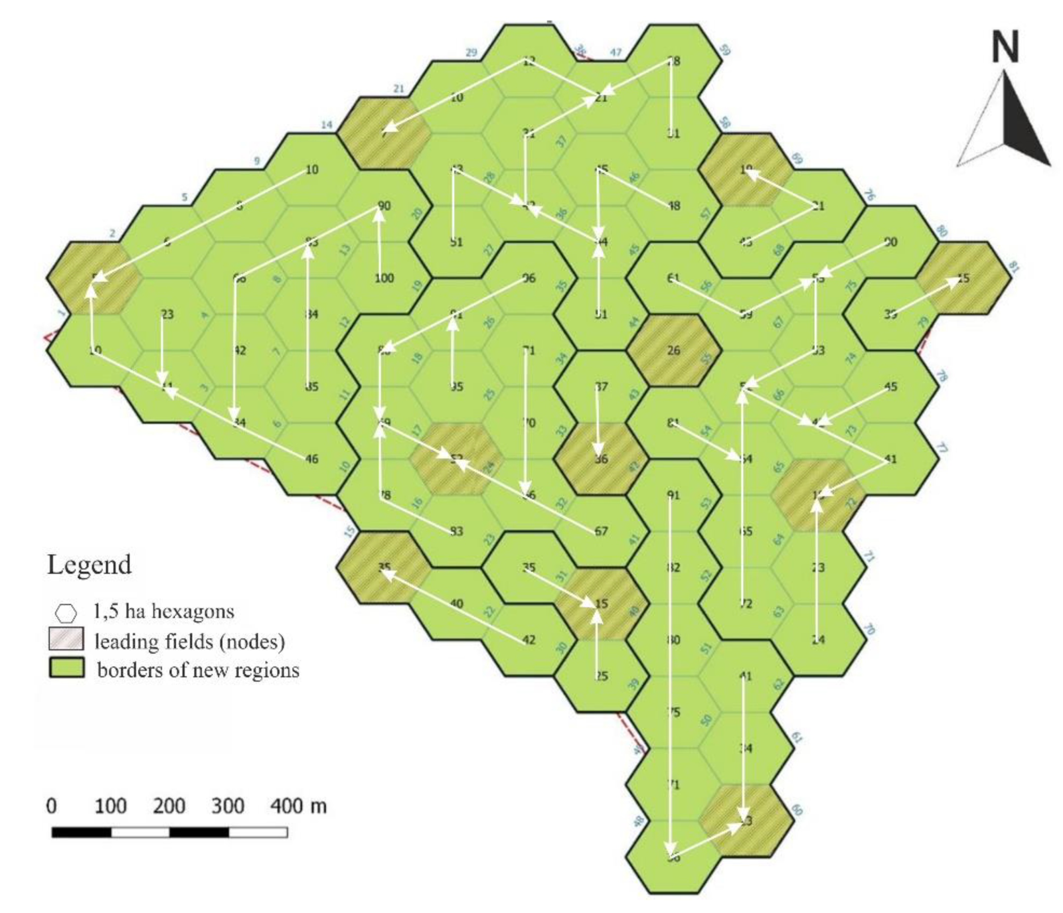
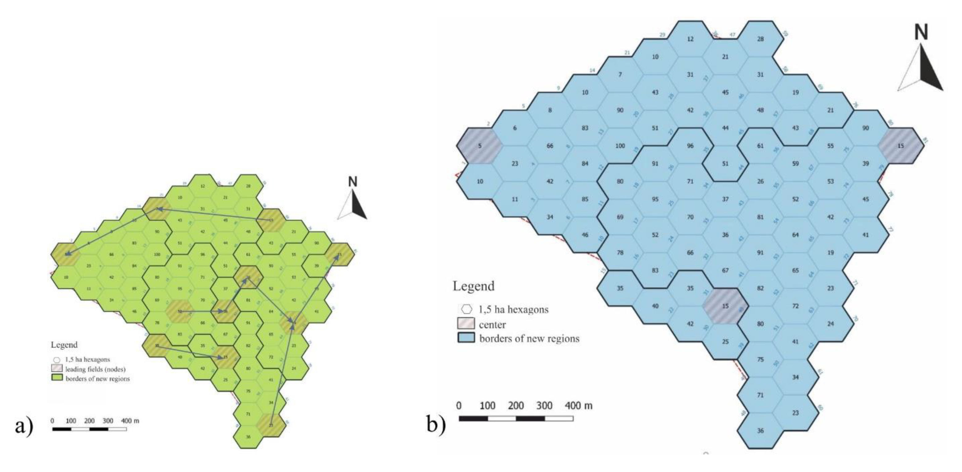
Connections in this network were generated based on the same principles as those previously described (i.e., to the neighboring field but according to the minimum value decrease principle). The stage of revealing relationships showed that for 84 fields (nodes; Figure 3a), the value decreases minimally and thus forms connections. Therefore, according to this path, stage 1 of aggregation enabled the emergence of 16 new regions (Figure 3b). In the next step of the model development, new regions (and their boundaries) were regarded as new nodes in the network, represented by the leading node’s value (definition in Section 2.1.1, p. 5). The values were combined in this way until the possibilities for a connection were exhausted (i.e., until the values could not be differentiated).
The minimum value decrease path revealed four value aggregation stages. Characteristics of the network model are provided in Table 4.
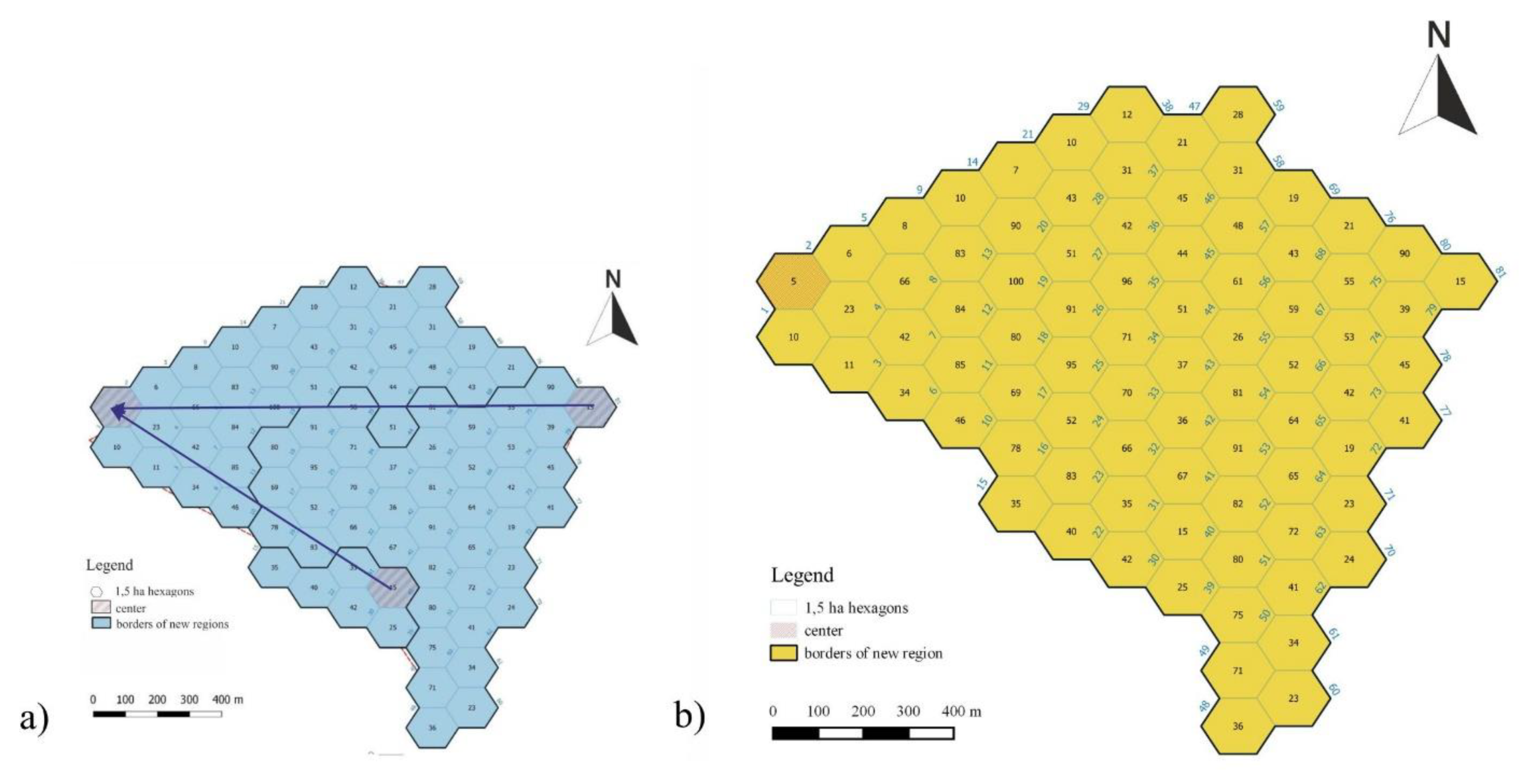
It should be noted that the final stage (i.e., the fourth stage of aggregation) resulted in the emergence of one region comprising 100 fields. A node generating a connection with all other nodes emerged (node No. 76).
With such assumptions and test data, a network model with a modular network structure and a maintained connection hierarchy was developed. In this network, since the formed connections have an orientation, it can be concluded that they only exist in one way. This is due to the fact that the minimum value decrease principle does not operate the other way around (e.g., Figure 3a); for example, field No. 2 will connect with field No. 12, but field No. 12 will not connect with field No. 2. Therefore, in the model interpretation, one can note nodes which have no connections at specific aggregation stages and a node which has 99 connections.
This reflects a situation where the orientation of connections generates the “channeling” (aggregation) of the studied phenomenon to nodes of a higher order (leading ones) until the possibilities for connection are exhausted. Network fields (nodes) to which a connection is established, achieve a higher rank in the network structure and become leading nodes that can achieve the degree of a node—the center of a particular network.
2.1.4. Maximum Value Decrease Path
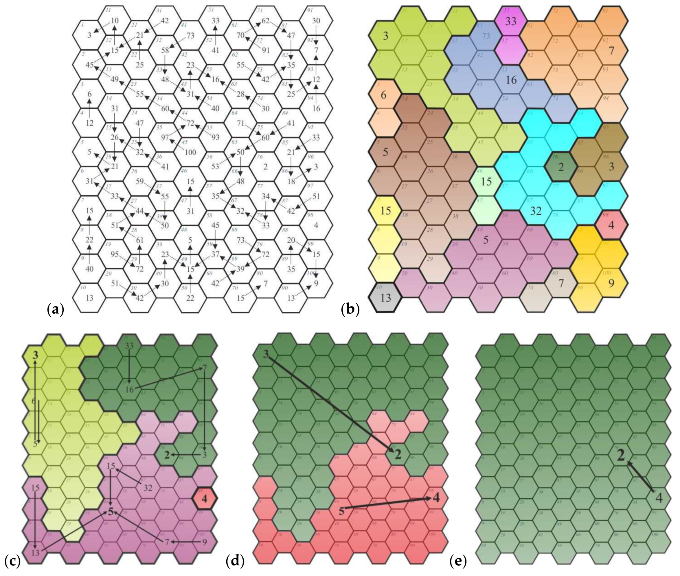
As regards this model, each field searched for a connection according to the maximum value decrease path. In this case, similar to Section 2.1.3, a hierarchical network model with modular structure elements was obtained as well. The network model comprises three stages of aggregation (Figure 4).
The stage of revealing relationships showed that for 84 fields (nodes; Figure 4a), the value decreases maximally and thus forms connections. In the first stage of aggregation, 16 new regions emerged, similar to the path of minimum value decrease (Figure 3b). However, the structure of the connections is different because the principle of connection was different. Characteristics of the network developed are provided in Table 5.
At the third stage of aggregation, three new regions emerged. This means that three leading nodes emerged in the network structure: one node with 14 connections, another one with 26 connections, and the last one with 57 connections. The fourth level aggregated all fields into one region. One node attracting (generating) 99 connections emerged (node No. 76).
2.1.5. Minimum Value Increase Path
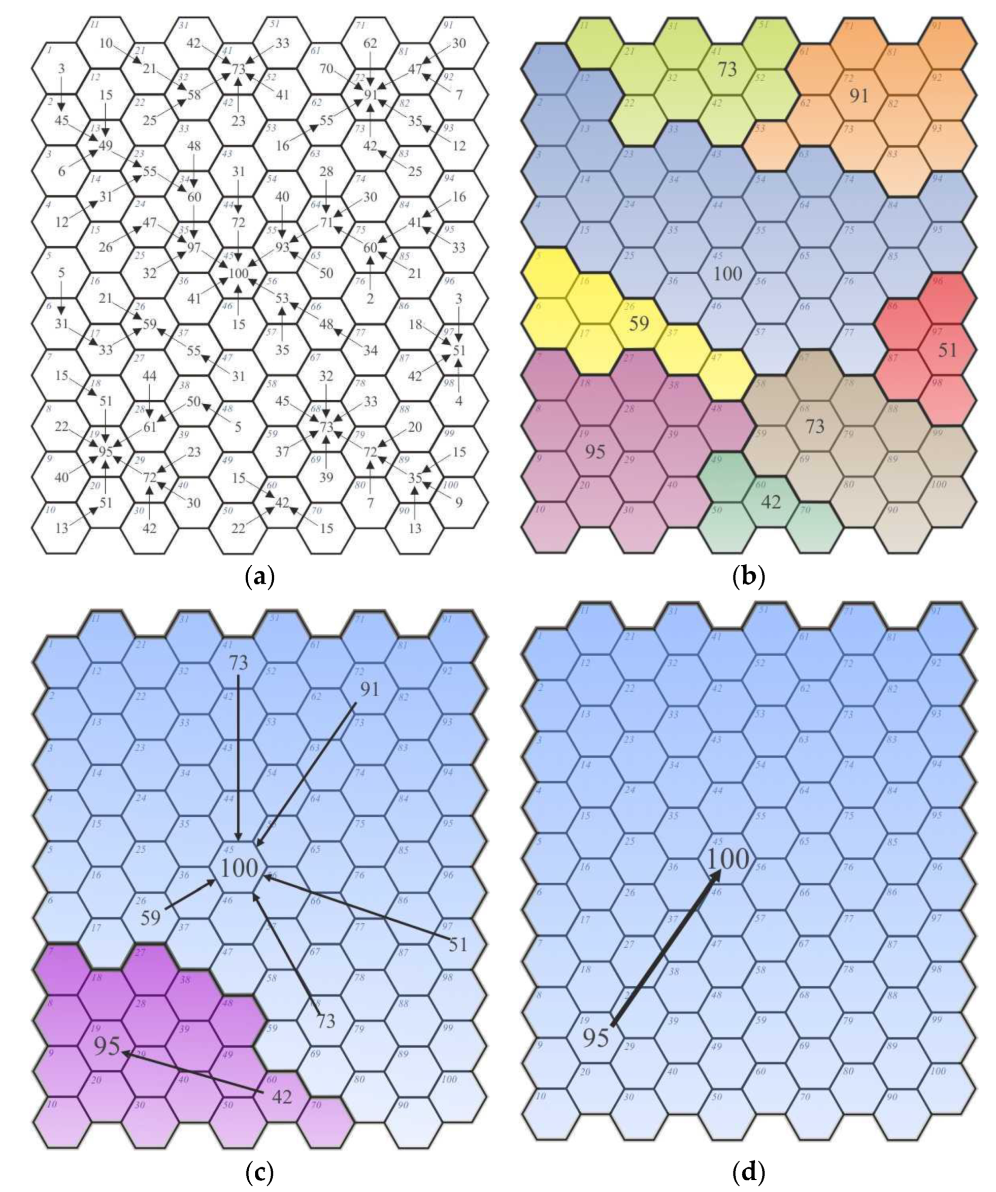
This path involves the development of a model of a network and new regions as a result of the generation of a connection of each field, in turn, with a selected neighboring field, according to the minimum value increase path. The regions which emerged due to the revealing of relationships search for new connections according to the same principles. The example provided below shows the emergence of a network in three aggregation stages (Figure 5).
At the stage of revealing relationships, 92 fields (nodes) found a connection according to the minimum value increase path (Figure 5a). In the first stage of aggregation, eight new regions emerged (Figure 5b). However, the structure of connections is different because the principle of connecting was different. Characteristics of the network developed are shown in Table 6.
The final (i.e., the third) stage of aggregation resulted in the emergence of one region comprising 100 fields. A node generating 99 connections emerged (node No. 45).
2.1.6. Maximum Value Increase Path
In this path, new regions emerged due to the generation of a connection between each field and the neighboring field as a result of maximum value increase. The diagram of the generation of networks and consequently, new regions, according to the maximum increase path is provided in Figure 6.
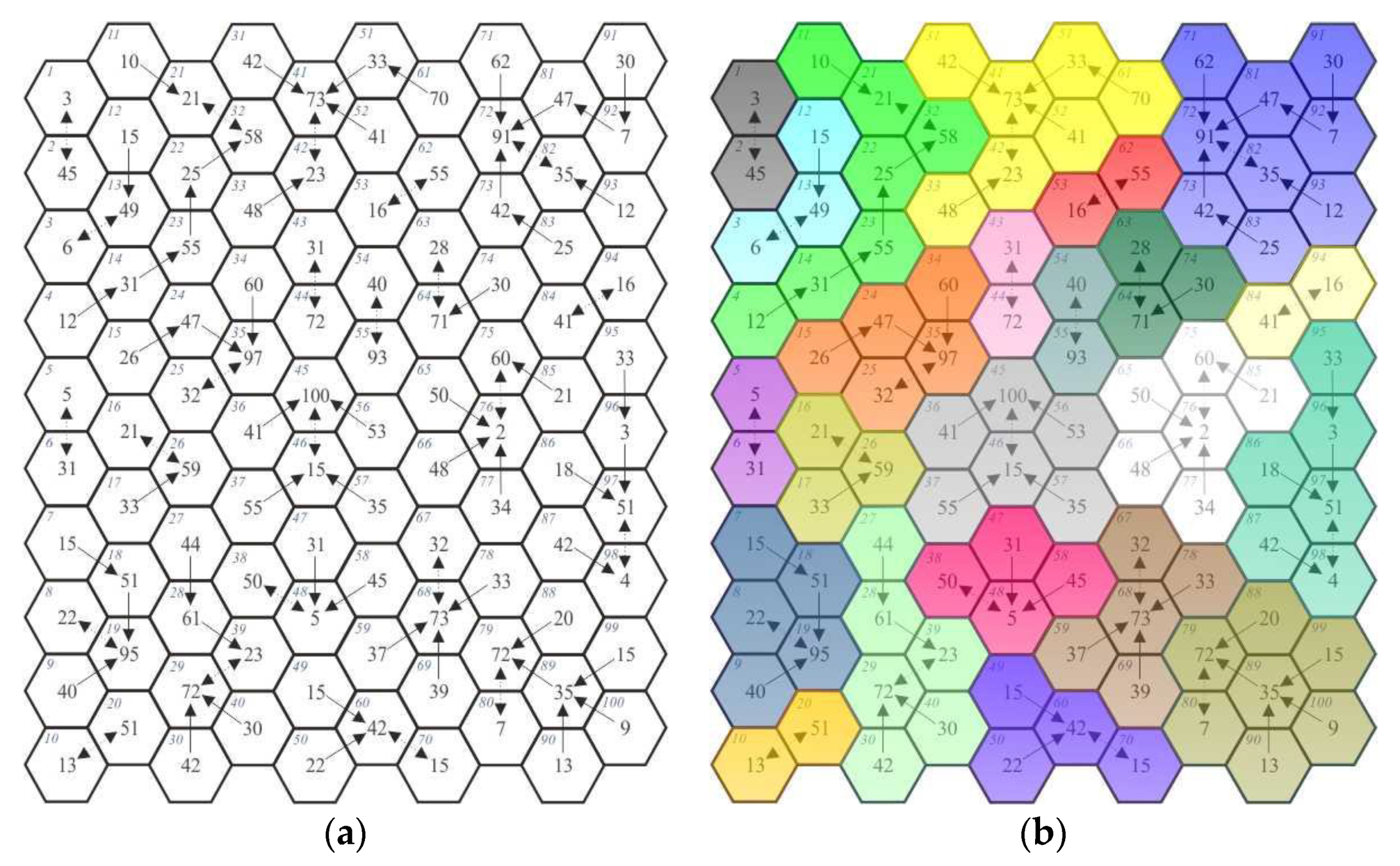
The above-presented network was developed in four stages (Figure 6). The first stage of revealing the maximum value increase relationship (Figure 6a) enabled the identification of 92 fields which achieved a connection. Thanks to these connections, eight new regions emerged at the first stage of value aggregation (Figure 6b), two at the second stage, and the third stage of aggregation resulted in a connection of 99 nodes to one (field/node No. 45). Characteristics of the network formed along with the number of nodes and connections are provided in Table 7.
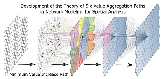
The network structure emerging in this way and the emergence of new connections (and, consequently, regions) can also be shown on a laminar model. As an example, Figure 7 shows particular levels of network emergence according to the maximum value increase path.
2.2. Network Models—Random or Scale-Free?
Having analyzed the process of network structure emergence according to the six proposed paths, it can be concluded that the entire structure of individual networks, depending on the specificity of values representing the fields and the path itself, emerges on a various number of aggregation stages. There are so many aggregation stages that the possibilities of connections according to the pre-determined paths and in line with the adopted principles (connection with the neighboring field) can be exhausted. In other words, the nodes represented by particular quantities are combined as long as a particular rule operates.
For the maximum and minimum difference paths, the possibility of combining all nodes into a single network is already exhausted after stage 1 of aggregation. This is due to the fact that at this level (stage 1 of aggregation), leading nodes in individual regions do not emerge for subsequent connections. New regions are formed which are represented in model terms by smaller network structures. For the minimum difference path, these are 26 network structures (Section 2.1.1, Figure 1b). In these structures, the maximum number of connections with a node amounts to seven. On the other hand, as regards the maximum difference path, in the first stage of aggregation 23 network structures, which formed new regions, emerged (Section 2.1.2, Figure 2b). In this case, the maximum number of connections with a node amounted to eight. It can therefore be concluded that at this stage these structures have a nature of random networks represented by normal distributions in which no nodes (i.e., centers) characteristic of scale-free structures can be distinguished. Therefore, these rules have no further application without changing the assumptions in subsequent steps. This is an issue to be addressed in further considerations. It also suggests that these two paths (rules of difference) are different from the subsequent four paths as they generate other rules at higher aggregation levels.
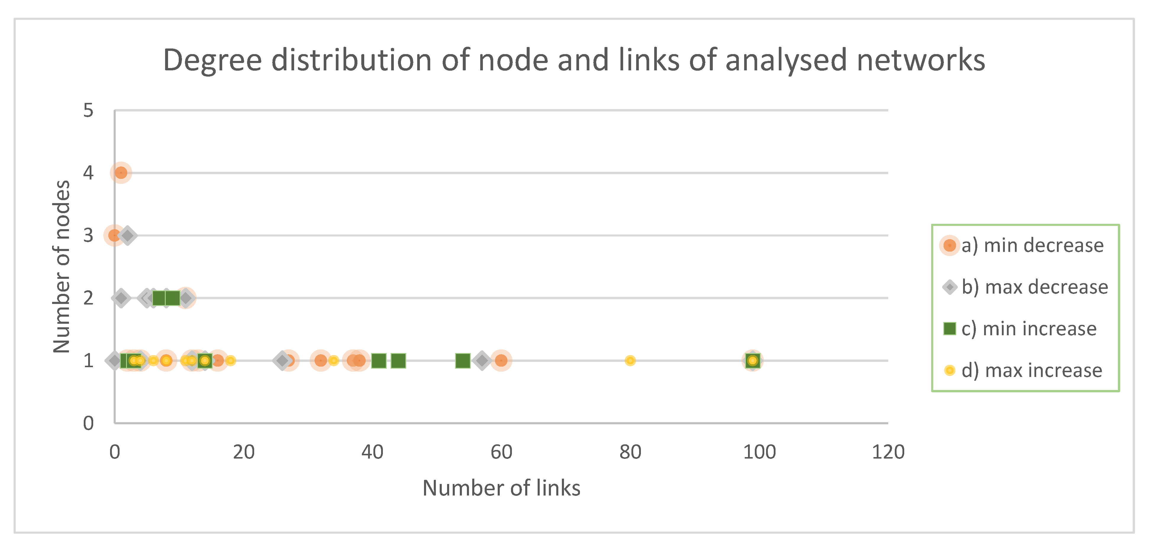
A different situation can be noticed after carrying out an analysis of the other four network structures developed according to the proposed rules of value decrease and increase. The figure provided below shows the distribution of nodes and connections in the structures of networks developed according to the six proposed paths (Figure 8).
The above distributions reveal the scale-free nature of the networks developed. Nodes are emerging which have a very large number of connections in relation to the majority. In such a structure, it is these nodes called centers that are most important. Their exclusion (destruction or damage) results in dysfunctionality in the operation of the entire network structure.
The structures developed according to the paths of minimum and maximum value decrease have features of a scale-free structure. This is indicated by the occurrence of nodes (i.e., centers or hubs) with a number of connections being much greater than the average (Figure 8a,b). The more connections a node or a center has, the more its weight in the functioning of the entire structure increases.
Moreover, having analyzed two subsequent distributions of nodes and connections (Figure 8c,d), it needs to be concluded that a scale-free structure is emerging in them. This is reflected by the outlying nodes (i.e., the centers of these networks).
Futuremore, nodes emerge that are of a lower weight than leading nodes (i.e., those with an average number of connections as compared to the majority). These nodes are an element that may predispose to the rank of centers. The more centers are present in the network structure, the more its resistance to deliberate attacks (dysfunctionality) increases. Therefore, the intermediate nodes are appropriate components whose rank, as a result of certain operations, may be elevated to that of centers by adding connections to them. A good example is an air connection network (a transport system) in which, due to the emergence of new connections on intermediate nodes and to the elevation of their rank up to that of a center, the entire network structure is more resistant to destruction. A condition for an increase in resistance is the conscious protection of the centers in these networks. Both the centers and intermediate nodes are rare components within the entire network structure.
A very important observation is that in four out of the six proposed paths, networks emerge whose nature is similar to that of scale-free networks. All of the analyzed paths fulfill one of the basic conditions for the emergence of scale-free networks (i.e., the preferential selection of connections). In scale-free networks, a weaker node searches for a stronger one to which it is profitable for it to connect within the structure of the existing network. It was assumed that in the analyzed structures, these nodes would connect to one another in accordance with the six rules.
3. Summary
The authors of the above-described theory assumed that a geoinformation analysis of the space for various purposes may be carried out using network modeling by six paths of value combination:
- -
- minimum value difference (Section 2.1.1),
- -
- maximum value difference (Section 2.1.2),
- -
- minimum value decrease (Section 2.1.3),
- -
- maximum value decrease (Section 2.1.4),
- -
- minimum value increase (Section 2.1.5),
- -
- maximum value increase (Section 2.1.6).
The values that are combined may represent various data. They may be assigned to a point but also to a specific basic field which includes a specific area and has a specific spatial reference. Therefore, the stage of data preparation for network modeling according to the theory of six paths involves the following:
- Step 1. Determination of the geoinformation analysis aim and the area under analysis;
- Step 2. Superimposition of a network of basic fields of assessment (e.g., hexagons);
- Step 3. Determination of values representing individual basic fields of assessment;
- Step 4. Network modeling according to the theory of six value combination paths, or according only to the paths that we consider to be appropriate (e.g., the minimum value decrease path);
- Step 5. Interpretation of the developed network models (random or scale-free) and an answer to the question about the achievement of the aim.
In the network models obtained in this way, nodes, leading nodes, and centers are distinguished. The most important are the centers of a particular network, as these are the critical points that are crucial to the functioning of the entire structure. These are the ones with the most connections as compared to the entire set. The removal of centers, or even some of them, may result in serious disturbances in the performance of a specific function.
Leading nodes are points of the network which are predisposed to the role of centers; these nodes can become centers through natural development as well as changes in the space and thus in the network structure. They can also transform into centers by means of conscious operations related to a change in the value in a basic field. These operations can be expressed by making changes within the space (i.e., increasing the aesthetic value of the landscape through building restoration, greenery arrangement, etc.) or the value representing the sense of one’s security (e.g., the application of Crime Prevention Through Environmental Design). In the network structures developed in this way, the connections which show with their orientation how the relationships between nodes are formed are important as well.
This theory, as each theory, has its limitations. One is the assumption that new regions emerge due to the generation of a connection between each field and a field that has a common boundary (a neighboring one). Each field can generate only one connection, but there are situations when neighboring fields have the same value. With this assumption we must make our choice of one of them. The situation in which more than one connection will be created leads to an uprising of “common” regions. One node or field belongs to more than one region. The complexity of this kind of model can be considered in the context of fuzzy set theory. This issue is in the research and analysis stage.
The theory of six value aggregation paths in network modeling for spatial analysis assumes that there are six paths of value connection. However, it is possible that along with the research and development of this theory, comparison with other theories and practical modeling, new possibilities (paths) of connections will be discovered.
Example of Application
One example of the application of the described rules of combining values according to the minimum and maximum value increase may be the modeling of recreational paths so that the aesthetic value of the landscape increases up to the points with the highest values (i.e., centers). This value may increase either minimally, which will result in a slower movement of the person walking and using the path, or maximally where the route developed on the basis of this network will lead the person to take the “shortcut” directly to the most attractive point within the area. In this case, the intermediate nodes are points with high, but not the highest, aesthetic values of the landscape. If there is a need to strengthen the network structure, the rank of these intermediate nodes may be elevated, as a result of operations aimed at landscape improvement, to that of centers (i.e., they can be deprived of their scale-free nature). A network with one center will operate differently than one with four centers. The more centers there are within a network structure, the more it is resistant to damage and dysfunctionality.
As regards the modeling of recreational paths, it is also reasonable to apply the path of the landscape aesthetic value minimum decrease. The authors present an example in five steps:
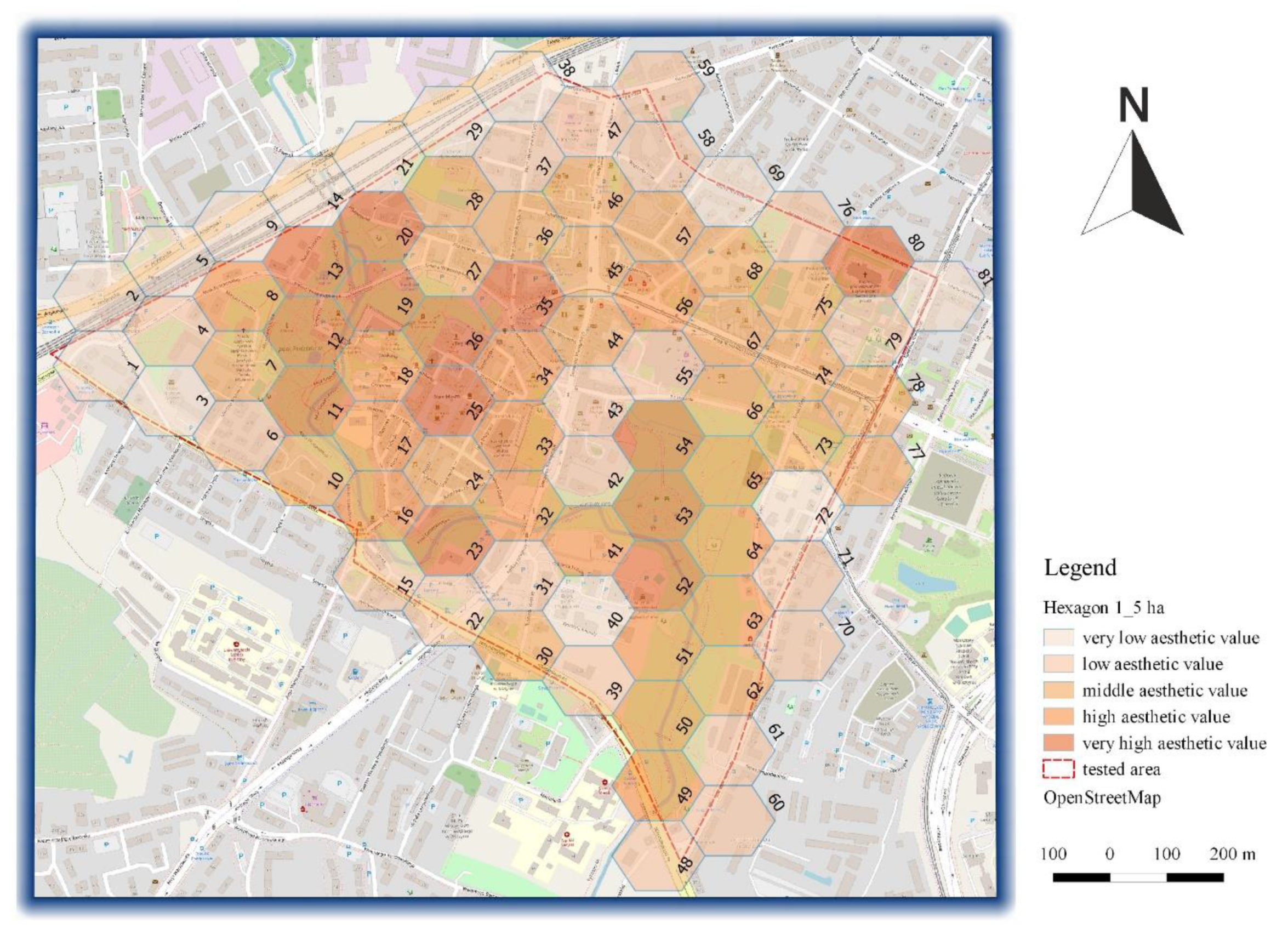
Step 1. Determination of the geoinformation analysis aim and the area under analysis: in this case, the aim of geoinformation analysis is to obtain spatial information about how the aesthetic value of the landscape in the area under study decreases, why it does so and how can this be remedied, and to show how not to plan recreational paths. The area under analysis is located in an urbanized area (a part of the city of Olsztyn in north-eastern Poland) with an area of approx. 120 ha (Figure 9).
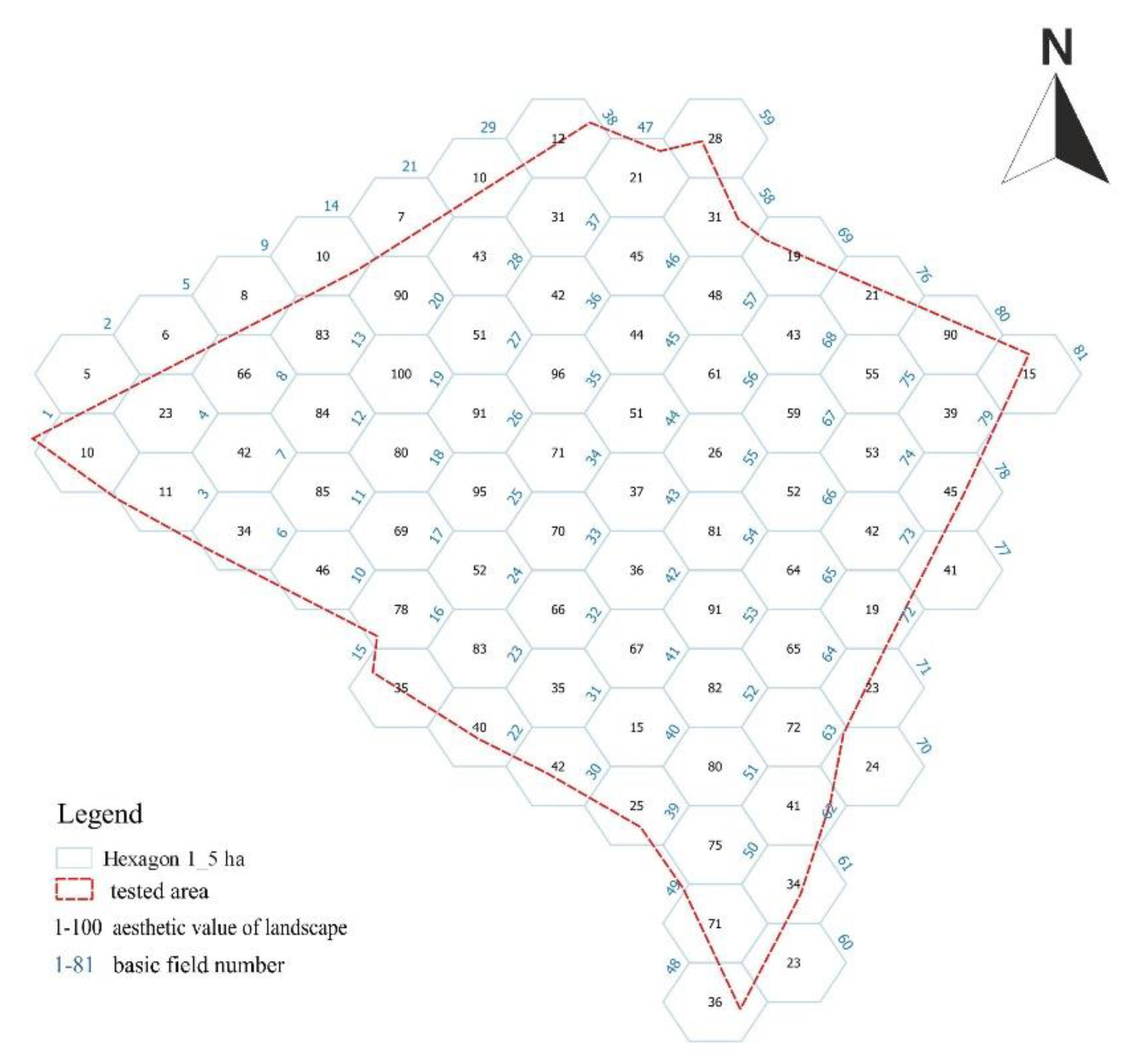
Step 2. Superimposition of the network of basic fields of assessment: a cartographic model presented using a hexbin map shows the basic fields of assessment in the shape of hexagons (a size of 1.5 ha each) (Figure 10).
Step 3. Determination of values representing individual basic fields of assessment: each hexagon presented in Figure 9 has its own number and an estimated aesthetic value of the landscape (the number provided in the central part of each field, on a scale ranging from 5 to 100). The values were estimated using the Wejchert method [47] and the filling in of an urban landscape assessment sheet.
Step 4. Network modeling using the minimum value decrease path (Figure 10, Figure 11, Figure 12 and Figure 13).
Step 5. Interpretation of the network models developed, and an answer to the question about the achievement of the aim.
The network model developed based on the rule of minimum decrease in value, in this case, the aesthetic value of a landscape, shows a situation where the landscape aesthetic value decreases minimally in relation to the neighboring fields (Figure 10, Figure 11, Figure 12 and Figure 13). This enables a very detailed analysis and explanation of even these slight differences in the landscape aesthetic value. Moreover, the fields that are the least attractive locally (i.e., the leading nodes) will be determined as well. By observing them we can pay attention to what makes the aesthetic value of the landscape so low and plan corrective measures. In this case, it will not be important to strengthen the leading nodes but to weaken them by increasing the value in a particular field. The subsequent aggregation levels show new value decrease paths and new nodes (Figure 12 and Figure 13) and ultimately, the center (Figure 13b). In this particular case, the center will be an area with the lowest aesthetic value of the landscape. Further operations making use of the developed network model and the properties of scale-free network should result in an increase in the landscape aesthetic value in the fields (i.e., in leading nodes) and the center. This will change the network structure and result in a change in connections by forming new leading nodes and centers. The operations related to increasing the landscape aesthetic value and network modeling should be continued until a satisfactory state of the space in the context of recreational path planning is achieved.
A maximum decrease model would present a situation where this value decreases maximally; it would, therefore, show connections within the network with a specific spatial location where, for various reasons, the landscape aesthetic value decreases drastically. It is, therefore, reasonable to develop models in accordance with particular paths individually and to superimpose them on one another in order to carry out subsequent spatial analyses and obtain geoinformation. They can be used for an analysis of the rate of changes in the landscape aesthetic value and the reasons for the decrease. They can also be used for operations aimed at increasing this value.
In order to optimally manage the landscape aesthetic value and, thus, increase city dwellers’ comfort of life, it appears reasonable to make use of all six value combination paths. The minimum and maximum difference paths show where the landscape value changes very little and where a significant change in relation to the neighborhood occurs. Part of the information which is revealed by these two paths is also shown in the remaining four paths related to value decrease and increase; the difference is that the different paths may show both an increase and decrease in the value. Such a model shows the rate of changes in landscape values and is a good tool to support planning and prediction of the space states, which allows the space to be used more optimally and erroneous decisions to be avoided, and thus enables the costs of error repairs to be avoided.
4. Conclusions
Spatial interactions that generate the network structure of the space, as a preference type, may result in the emergence of spatial scale-free networks. By modeling the space in this way and analyzing the model, the evolution of the network structure can be, within a specified scope, controlled. These operations include the formation of new nodes and connections and the use of network properties depending on what their character is (random or scale-free) and their structure (e.g., modular or hierarchical).
As for scale-free networks, the establishment of connections between objects takes place, in a sense, without spatial limitations. A spatially separated object (with no common “boundary”) may establish a connection with another one; examples include air connection networks, Internet networks, or social cooperation networks.
As regards the emergence of spatial networks forming compact regions, these connections must be made in relation to the immediate neighbors on the agglomeration path. The preferential selection applies as in scale-free networks and is carried out according to the rules of the six value aggregation paths described and defined in this article yet is oriented towards the neighboring objects (areas).
The first two rules of aggregation of a minimum and maximum difference generate only one aggregation level and do not result in the emergence of one hierarchical network with modular network characteristics. These rules model particular values to form them into small networks of a random nature, in which no centers can be distinguished. These models can be used to carry out preliminary analyses and to show where the values representing the state of the space change very little, and where a significant change occurs in relation to the neighborhood. Unlike the rules related to a value decrease or increase, the rule of value difference, irrespective of whether minimum or maximum, always applies.
The four subsequent four aggregation rules in the modeling of planning space network structures related to the increase and decrease in the values being modeled enabled the development of network models whose nature is similar to that of scale-free networks. This indicates the power-law distribution of nodes and connections, and the possibility of the identification of centers within the structures of these networks.
The proposed methods for modeling spatial data described above enable the imaging of not only a stable picture of the state of the space but also changes in the states of this space. In this way, it is possible to cartographically image (model) the distribution of values of interesting issues related to the state and management of the space (e.g., the landscape aesthetic value, real estate value, noise level, safety level, and the space investment level). An added value of modeling according to the six proposed paths is the indication of relationships between the data being modeled, which provides additional geoinformation and enables additional conclusions to be drawn. Moreover, it provides answers not only to the question “where?” but also “why?” and “what to do with it?” Such modeling also allows the scale-free network features to be used to identify centers within the network (i.e., the most important nodes) for the operation of the entire structure.
Subsequent studies will involve the application of the six described rules of aggregation paths for geodata modeling and the development of complex models. The utility of the application of combined models based on the geoinformation they provide will then be assessed.
The models developed according to the theory described above present the quality of urban areas in its various versions. The theory of six paths of value combination includes the new measuring tools and methods which can have an impact on the quality of life and minimize the costs of bad design or spatial destruction. They are also a proper tool for the sustainable development of urban areas.
Author Contributions
Conceptualization, Anna Maria Kowalczyk and Tomasz Bajerowski; Formal analysis, Anna Maria Kowalczyk; Methodology, Anna Maria Kowalczyk and Tomasz Bajerowski; Visualization, Anna Maria Kowalczyk. All authors have read and agreed to the published version of the manuscript.
Funding
This research received no external funding.
Conflicts of Interest
The authors declare no conflicts of interest.
References
- Christaller, W. Central Places in Southern Germany; Prentice-Hall: Upper Saddle River, NJ, USA, 1966. [Google Scholar]
- Domański, R. Teoretyczne Podstawy Geografii Ekonomicznej; Państwowe Wydawnictwo Ekonomiczne: Warsaw, Poland, 1987. [Google Scholar]
- Allmendinger, P.; Haughton, G. Spatial planning, devolution, and new planning spaces. Environ. Plan. C Gov. Policy 2010, 28, 803–818. [Google Scholar] [CrossRef]
- Euler, L. Leonhard Euler and the Königsberg bridges. Sci. Am. 1953, 189, 66–70. [Google Scholar] [CrossRef]
- Steinhaus, H.; Łukaszewicz, J. O wyznaczaniu środka miedzi sieci telefonicznej. Appl. Math. 1953, 1, 299–307. [Google Scholar] [CrossRef]
- Barabási, A.L. Linked: The New Science of Networks; Perseus Books Group: New York, NY, USA, 2003. [Google Scholar]
- Acid, S.; de Campos, L.M. Searching for Bayesian network structures in the space of restricted acyclic partially directed graphs. J. Artif. Intell. Res. 2003, 18, 445–490. [Google Scholar] [CrossRef]
- Newman, M.; Barabasi, A.L.; Watts, D.J. The Structure and Dynamics of Networks; Princeton University Press: Princeton, NJ, USA, 2011. [Google Scholar]
- Kiełkowicz, K.; Kokosiński, Z. Algorytm hybrydowy dla probabilistycznego problemu komiwojażera. Czas. Tech. Autom. 2012, 109, 115–126. [Google Scholar]
- Kowalczyk, A. The iconic model of landscape aesthetic value. Eur. Spat. Res. Policy 2012, 19, 121–128. [Google Scholar] [CrossRef] [Green Version]
- Bajerowski, T.; Kowalczyk, A.M. Metody Geoinformacyjnych Analiz Jawnoźródłowych w Zwalczaniu Terroryzmu; Wydawnictwo Uniwersytetu Warmińsko-Mazurskiego: Olsztyn, Poland, 2013. [Google Scholar]
- Biłozor, A.; Kowalczyk, A.M.; Bajerowski, T. Theory of Scale-Free Networks as a New Tool in Researching the Structure and Optimization of Spatial Planning. J. Urban Plan. Dev. 2018, 144, 04018005. [Google Scholar] [CrossRef]
- Goldberg, A.V.; Radzik, T. A heuristic improvement of the Bellman-Ford algorithm. Appl. Math. Lett. 1993, 6, 3–6. [Google Scholar] [CrossRef] [Green Version]
- Applegate, D.; Bixby, R.; Chvátal, V.; Cook, W. Implementing the Dantzig-Fulkerson-Johnson algorithm for large traveling salesman problems. Math. Program. 2003, 97, 91–153. [Google Scholar] [CrossRef]
- Guttoski, P.B.; Sunye, M.S.; Silva, F. Kruskal’s algorithm for query tree optimization. In Proceedings of the 11th International Database Engineering and Applications Symposium (IDEAS 2007), Banff, AB, Canada, 6–8 September 2007; pp. 296–302. [Google Scholar]
- Zhan, F.B. Three fastest shortest path algorithms on real road networks: Data structures and procedures. J. Geogr. Inf. Decis. Anal. 1997, 1, 69–82. [Google Scholar]
- Erdös, P.; Rényi, A. On random graphs. Publ. Math. 1959, 6, 290–297. [Google Scholar]
- Erdös, P.; Rényi, A. On the evolution of random graphs. Publ. Math. Inst. Hung. Acad. Sci. 1960, 5, 17–60. [Google Scholar]
- Békéssy, A. Asymptotic enumeration of regular matrices. Stud. Sci. Math. Hung. 1972, 7, 343–353. [Google Scholar]
- Bender, E.A.; Canfield, E.R. The asymptotic number of labelled graphs with given degree sequences. J. Comb. Theory A 1978, 24, 296. [Google Scholar] [CrossRef] [Green Version]
- Bollobás, B. A probabilistic proof of an asymptotic formula for the number of labelled regular graphs. Eur. J. Comb. 1980, 1, 311–316. [Google Scholar] [CrossRef] [Green Version]
- Bollobás, B. Modern Graph Theory; Springer Science & Business Media: Berlin/Heidelberg, Germany, 2013; Volume 184. [Google Scholar]
- Wormald, N.C. The asymptotic connectivity of labelled regular graphs. J. Comb. Theory B 1981, 31, 156–167. [Google Scholar] [CrossRef] [Green Version]
- Watts, D.J.; Strogatz, S.H. Collective dynamics of ‘small-world’ networks. Nature 1998, 393, 440. [Google Scholar] [CrossRef]
- Barabási, A.L.; Albert, R. Emergence of scaling in random networks. Science 1999, 286, 509–512. [Google Scholar] [CrossRef] [Green Version]
- Barabási, A.L.; Ravasz, E.; Vicsek, T. Deterministic scale-free networks. Phys. A Stat. Mech. Appl. 2001, 299, 559–564. [Google Scholar] [CrossRef] [Green Version]
- Dorogovtsev, S.N.; Mendes, J.F. Evolution of Networks: From Biological Nets to the Internet and WWW; OUP: Oxford, UK, 2013. [Google Scholar]
- Kowlaczyk, A. The analysis of networks space structures as important elements of sustainable space development. In Proceedings of the 10th International Conference “Environmental Engineering” 2017, Vilnius, Lithuania, 27–28 April 2017. [Google Scholar]
- Costa, L.D.F.; Rodrigues, F.A.; Travieso, G.; Villas Boas, P.R. Characterization of complex networks: A survey of measurements. Adv. Phys. 2007, 56, 167–242. [Google Scholar] [CrossRef] [Green Version]
- Renssen, H.; Knoop, J.M. A global river routing network for use in hydrological modeling. J. Hydrol. 2000, 230, 230–243. [Google Scholar] [CrossRef]
- Abe, S.; Suzuki, N. Scale-free network of earthquakes. EPL Europhys. Lett. 2004, 65, 581. [Google Scholar] [CrossRef] [Green Version]
- Kowalczyk, A.M. The use of scale-free networks theory in modelling landscape aesthetic value networks in urban areas. Geod. Vestn. 2015, 59, 135–152. [Google Scholar] [CrossRef]
- Wang, W.X.; Wang, B.H.; Yin, C.Y.; Xie, Y.B.; Zhou, T. Traffic dynamics based on local routing protocol on a scale-free network. Phys. Rev. E 2006, 73, 026111. [Google Scholar] [CrossRef] [Green Version]
- Kocur-Bera, K. Scale-free network theory in studying the structure of the road network in Poland. Promet-Traffic Transp. 2014, 26, 235–242. [Google Scholar] [CrossRef]
- Schvaneveldt, R.W.; Durso, F.T.; Dearholt, D.W. Network structures in proximity data. In Psychology of Learning and Motivation; Academic Press: Cambridge, MA, USA, 1989; Volume 24, pp. 249–284. [Google Scholar]
- Laireiter, A.; Baumann, U. Network Structures and Support Functions: Theoretical and Empirical Analyses; Hemisphere Publishing Corp.: London, UK, 1992. [Google Scholar]
- Barabási, A.L.; Bonabeau, E. Scale-free networks. Sci. Am. 2003, 288, 60–69. [Google Scholar] [CrossRef]
- Vazquez, A. Exact results for the Barabási model of human dynamics. Phys. Rev. Lett. 2005, 95, 248701. [Google Scholar] [CrossRef] [Green Version]
- Bednarczyk, M.; Kowalczyk, K.; Kowalczyk, A.M. Identification of pseudo-nodal points on the basis of precise leveling campaigns data and GNSS. Acta Geodyn. Geomater. 2018, 15, 5–16. [Google Scholar] [CrossRef] [Green Version]
- Kowalczyk, A.M. The analysis and creation of landscape aesthetic value network models as important elements of sustainable urban development. In Environmental Engineering. Proceedings of the International Conference on Environmental Engineering. ICEE; Vilnius Gediminas Technical University, Department of Construction Economics & Property: Vilnius, Lithuania, 2014; Volume 9, p. 1. [Google Scholar]
- Kowalczyk, A.; Kowalczyk, K. The network theory in the process of creating and analyzing from vertical crustal movements. In Proceedings of the 14th GeoConference on Informatics, Geoinformatics and remote Sensing, Albena, Bulgaria, 17–26 June 2014; pp. 545–552. [Google Scholar]
- Bajerowski, T.; Kowalczyk, A.M.; Ogrodniczak, M. Network structures in developing uniformed service intervention maps. SGEM Surv. Geol. Min. Ecol. Manag. 2017, 17, 619–624. [Google Scholar]
- Papageorgiou, G.J. Agglomeration. Reg. Sci. Urban Econ. 1979, 9, 41–59. [Google Scholar] [CrossRef]
- Chuanglin, F.A.N.G. Research progress and general definition about identification standards of urban agglomeration space. In Urban Planning Forum; Tongji University: Shanghai, China, 2009; Volume 4, pp. 1–6. [Google Scholar]
- Johansson, B.; Quigley, J.M. Agglomeration and networks in spatial economics. Pap. Reg. Sci. 2004, 83, 165–176. [Google Scholar] [CrossRef] [Green Version]
- Hopfer, A.; Cymerman, R.; Nowak, A. Ocena i Waloryzacja Gruntów Wiejskich; Państwowe Wydaw. Rolnicze i Leśne: Warsaw, Poland, 1982. [Google Scholar]
- Bajerowski, T.; Biłozor, A.; Cieślak, I.; Senetra, A.; Szczepańska, A. Ocena i Wycena Krajobrazu; Wyd. Educaterra: Olsztyn, Poland, 2007. [Google Scholar]
- Senetra, A.; Cieślak, I. Kartograficzne Aspekty Oceny i Waloryzacji Przestrzeni; Wydaw. Uniwersytetu Warmińsko-Mazurskiego: Olsztyn, Poland, 2004. [Google Scholar]
- Lechnio, J. Jednostki krajobrazowe jako pola podstawowe oceny zagrożenia środowiska przyrodniczego depozycja substancji zakwaszajacych. Problemy Ekologii Krajobrazu 2004, 12. [Google Scholar]
- ResearchGate. 2019. Available online: https://www.researchgate.net/figure/Hex-bin-map-of-the-formulated-Change-Index-for-the-long-term-scenario-Each-hexagon_fig5_331863624 (accessed on 11 February 2020).
Figure 1.
The stages of network emergence according to the minimum value difference path: (a) the stage of revealing the minimum difference relationship, and (b) the first stage of value aggregation and the emergence of new regions. Source: Own analysis.
Figure 1.
The stages of network emergence according to the minimum value difference path: (a) the stage of revealing the minimum difference relationship, and (b) the first stage of value aggregation and the emergence of new regions. Source: Own analysis.
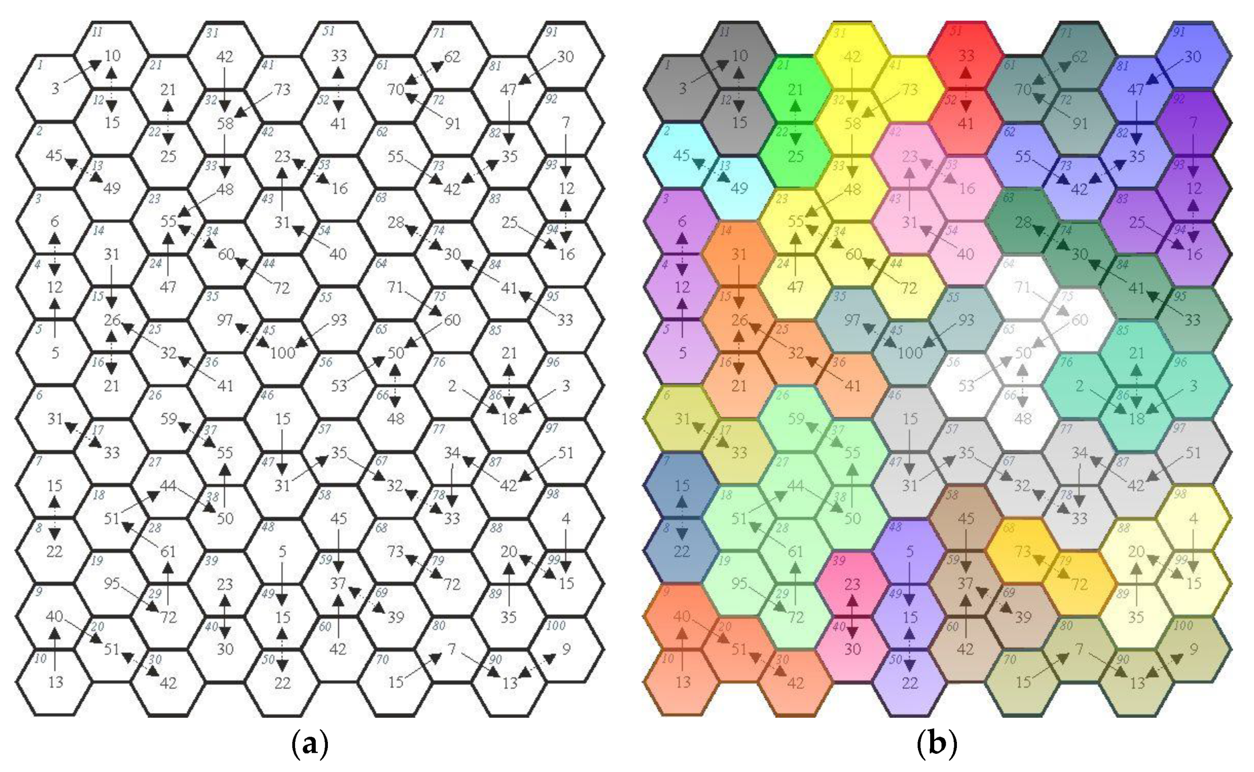
Figure 2.
The stages of network emergence according to the maximum value difference path: (a) the stage of revealing the maximum difference relationship; (b) the first stage of value aggregation and the emergence of new regions. Source: Own analysis.
Figure 2.
The stages of network emergence according to the maximum value difference path: (a) the stage of revealing the maximum difference relationship; (b) the first stage of value aggregation and the emergence of new regions. Source: Own analysis.

Figure 3.
The stages of network emergence according to the minimum value decrease path: (a) the stage of revealing the minimum value decrease relationship; (b) the first stage of value aggregation; (c) the second stage of value aggregation; (d) the third stage of value aggregation; (e) the fourth stage of value aggregation.

Figure 4.
The stages of network emergence according to the maximum value decrease path: (a) the stage of revealing the maximum value decrease relationship; (b) the first stage of value aggregation; (c) the second stage of value aggregation; (d) the third stage of value aggregation. Source: Own analysis.
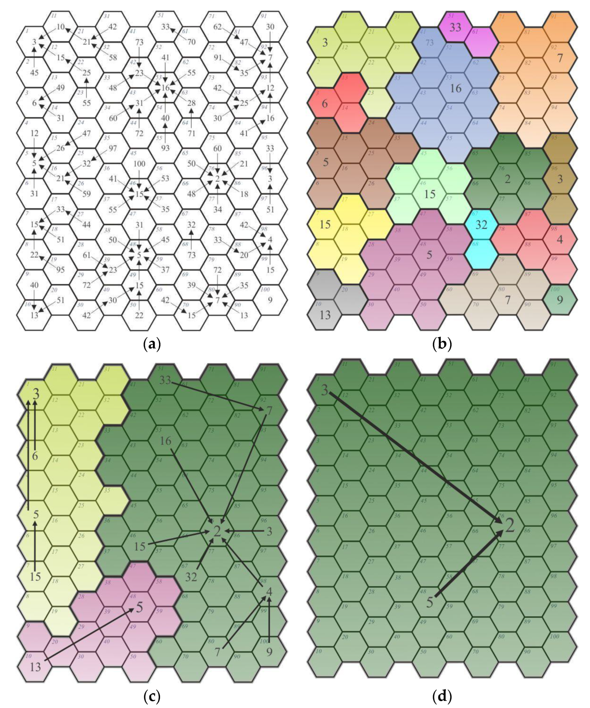
Figure 5.
The stages of network emergence according to the minimum value increase path: (a) the stage of revealing the minimum value increase relationship; (b) the first stage of value aggregation; (c) the second stage of value aggregation; (d) the third stage of value aggregation. Source: Own analysis.
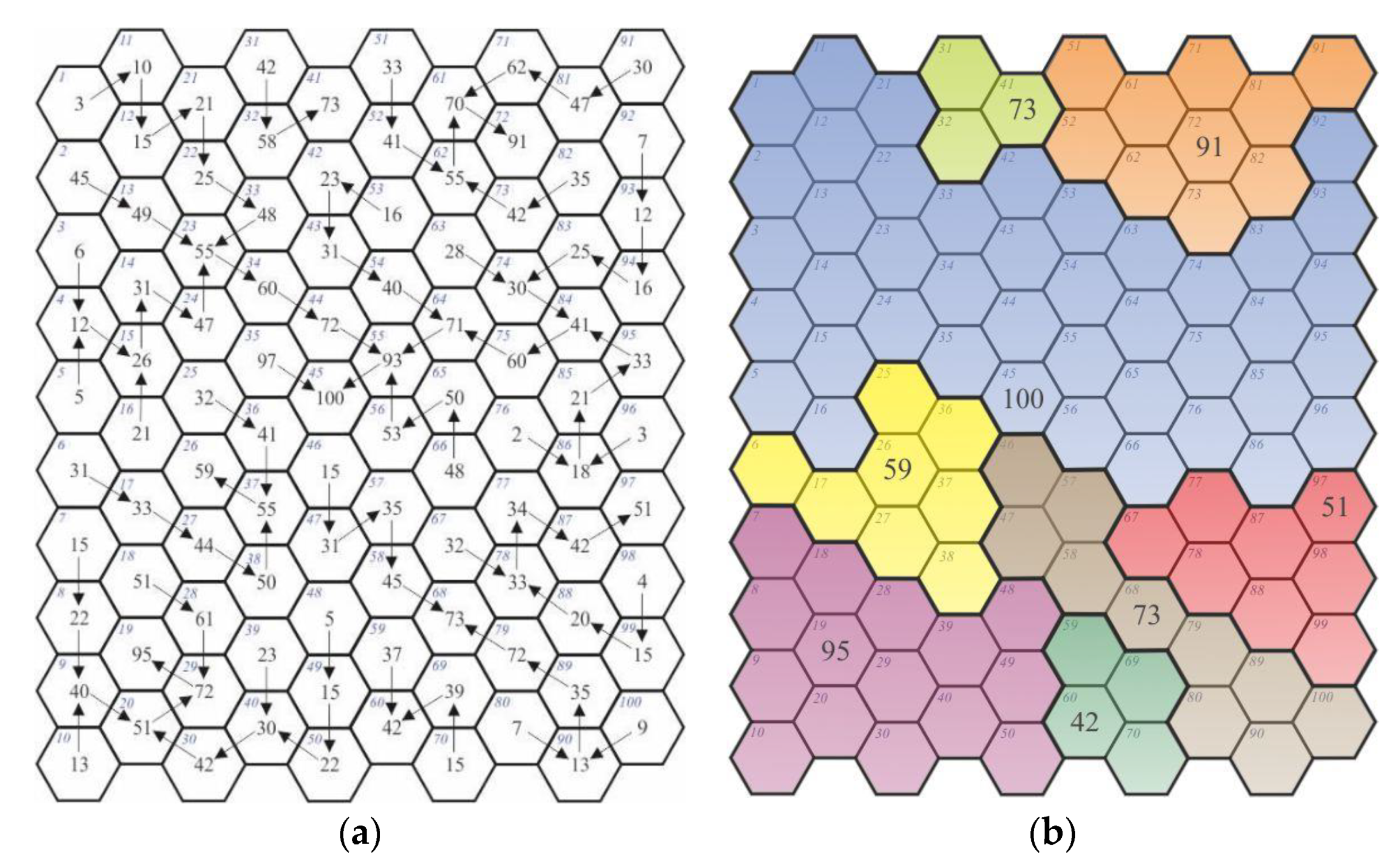
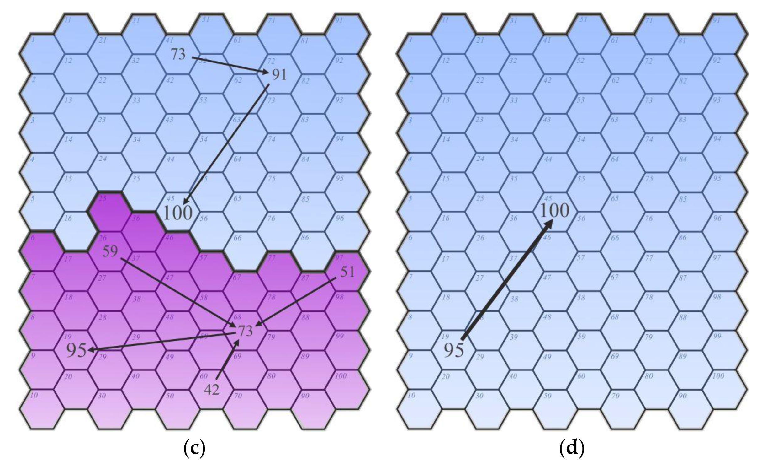
Figure 6.
The levels of emergence of networks and new spatial regions according to the maximum value increase path: (a) the stage of revealing the minimum value increase relationship; (b) the first stage of value aggregation; (c) the second stage of value aggregation; (d) the third stage of value aggregation. Source: Own analysis.

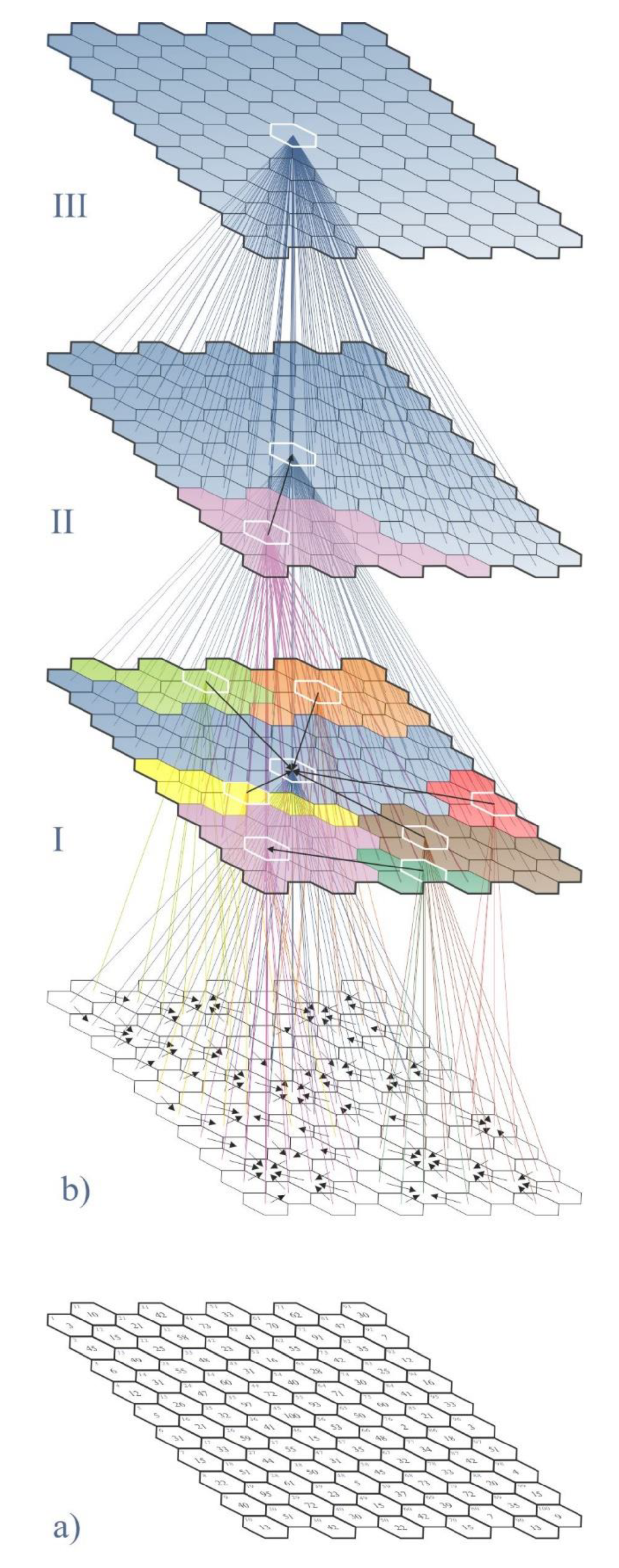
Figure 7.
The levels of network emergence according to the path of maximum increase in the spatial interaction indicator (aggregation levels): (a) basic fields with the assigned values that reflect a studied phenomenon; (b) the stage of revealing relationships; in this case, the maximum value increase; (I) the first stage of value aggregation according to the maximum value increase path; (II) the second stage of value aggregation according to the maximum value increase path; (III) the third stage of value aggregation according to the maximum value increase path. Source: Own analysis.

Figure 8.
The distribution of nodes and links in the developed network structures. Key: Network models developed according to the paths of (a) minimum value decrease; (b) maximum value decrease; (c) minimum value increase; (d) maximum value increase. Source: Own analysis.
Figure 8.
The distribution of nodes and links in the developed network structures. Key: Network models developed according to the paths of (a) minimum value decrease; (b) maximum value decrease; (c) minimum value increase; (d) maximum value increase. Source: Own analysis.

Figure 9.
The area of analysis. Hexbin map of aesthetic value needed for network modeling. Source: Own analysis in QGis and based on Open Street Map data.
Figure 9.
The area of analysis. Hexbin map of aesthetic value needed for network modeling. Source: Own analysis in QGis and based on Open Street Map data.

Figure 10.
The stage of revealing the relationships of the minimum landscape aesthetic value decrease. Source: Own analysis.
Figure 10.
The stage of revealing the relationships of the minimum landscape aesthetic value decrease. Source: Own analysis.

Figure 11.
The first stage of aggregation of the landscape aesthetic value according to the minimum value decrease path. Key: white arrows show how the landscape aesthetic value decreases minimally.
Figure 11.
The first stage of aggregation of the landscape aesthetic value according to the minimum value decrease path. Key: white arrows show how the landscape aesthetic value decreases minimally.

Figure 12.
The second stage of aggregation of the landscape aesthetic value according to the minimum value decrease path; (a) the combination of values according to the principle of minimum value decrease; (b) new regions.
Figure 12.
The second stage of aggregation of the landscape aesthetic value according to the minimum value decrease path; (a) the combination of values according to the principle of minimum value decrease; (b) new regions.

Figure 13.
The third stage of aggregation of the landscape aesthetic value according to the minimum value decrease path; (a) the combination of values according to the principle of minimum value decrease; (b) new regions.
Figure 13.
The third stage of aggregation of the landscape aesthetic value according to the minimum value decrease path; (a) the combination of values according to the principle of minimum value decrease; (b) new regions.


Table 1.
General characteristics of random networks and scale-free networks.
| Random Networks | Scale-Free Networks |
|---|---|
|
|
 |  |
|
|
|
|
|
|
|
|
|
|
Table 2.
Characteristics of the structure of networks formed according to the minimum value difference path.
Table 2.
Characteristics of the structure of networks formed according to the minimum value difference path.
| Number of Regions: 26, Including: | Number of Fields (Nodes) | Number of Connections | |
|---|---|---|---|
| Stage 1 of aggregation | 7 | 2 | 1 |
| 5 | 3 | 2 | |
| 8 | 4 | 3 | |
| 3 | 5 | 4 | |
| 3 | 8 | 7 |
Source: Own analysis.
Table 3.
Characteristics of the structure of networks formed according to the maximum value difference path.
Table 3.
Characteristics of the structure of networks formed according to the maximum value difference path.
| Number of Regions: 23, Including: | Number of Fields (Nodes) | Number of Connections | |
|---|---|---|---|
| Stage 1 of aggregation | 7 | 2 | 1 |
| 3 | 3 | 2 | |
| 2 | 4 | 3 | |
| 3 | 5 | 4 | |
| 4 | 6 | 5 | |
| 3 | 7 | 6 | |
| 1 | 9 | 8 (node No. 72) |
Source: Own analysis.
Table 4.
Characteristics of the structure of networks formed according to the minimum value decrease path.
Table 4.
Characteristics of the structure of networks formed according to the minimum value decrease path.
| Number of Regions | Number of Fields (Nodes) | Number of Connections | |
|---|---|---|---|
| Stage 1 of aggregation 16 regions emerged (16R) | 3 | 1 | 0 |
| 4 | 2 | 1 | |
| 1 | 3 | 2 | |
| 1 | 4 | 3 | |
| 1 | 5 | 4 | |
| 1 | 9 | 8 | |
| 2 | 12 | 11 | |
| 1 | 13 | 12 | |
| 1 | 14 | 13 | |
| 1 | 17 | 16 | |
| Stage 2 of aggregation (4R) | 1 | 1 | 0 |
| 1 | 28 | 27 | |
| 1 | 33 | 32 | |
| 1 | 38 | 37 | |
| Stage 3 of aggregation (2R) | 1 | 39 | 38 |
| 1 | 61 | 60 | |
| Stage 4 of aggregation (1R) | 1 | 100 | 99 (node No. 76) |
Source: Own analysis.
Table 5.
Characteristics of the structure of networks formed according to the maximum value decrease path.
Table 5.
Characteristics of the structure of networks formed according to the maximum value decrease path.
| Number of Regions | Number of Fields (Nodes) | Number of Connections | |
|---|---|---|---|
| Stage 1 of aggregation 16 regions emerged (16R) | 1 | 1 | 0 |
| 2 | 2 | 1 | |
| 3 | 3 | 2 | |
| 1 | 5 | 4 | |
| 2 | 6 | 5 | |
| 2 | 7 | 6 | |
| 2 | 9 | 8 | |
| 2 | 12 | 11 | |
| 1 | 13 | 12 | |
| Stage 2 of aggregation (3R) | 1 | 15 | 14 |
| 1 | 27 | 26 | |
| 1 | 58 | 57 | |
| Stage 3 of aggregation (1R) | 1 | 100 | 99 (node No. 76) |
Source: Own analysis.
Table 6.
Characteristics of the structure of networks formed according to the minimum value increase path.
Table 6.
Characteristics of the structure of networks formed according to the minimum value increase path.
| Number of Regions | Number of Fields (Nodes) | Number of Connections | |
|---|---|---|---|
| Stage 1 of aggregation 8 regions emerged (8R) | 1 | 3 | 2 |
| 1 | 4 | 3 | |
| 2 | 8 | 7 | |
| 2 | 10 | 9 | |
| 1 | 15 | 14 | |
| 1 | 42 | 41 | |
| Stage 2 of aggregation (2R) | 1 | 45 | 44 |
| 1 | 55 | 54 | |
| Stage 3 of aggregation (1R) | 1 | 100 | 99 (node No. 45) |
Source: Own analysis.
Table 7.
Characteristics of the structure of networks formed according to the maximum value increase path.
Table 7.
Characteristics of the structure of networks formed according to the maximum value increase path.
| Number of Regions | Number of Fields (Nodes) | Number of Connections | |
|---|---|---|---|
| Stage 1 of aggregation 8 regions emerged (8R) | 1 | 4 | 3 |
| 1 | 5 | 4 | |
| 1 | 7 | 6 | |
| 1 | 9 | 8 | |
| 1 | 12 | 11 | |
| 1 | 13 | 12 | |
| 1 | 15 | 14 | |
| 1 | 35 | 34 | |
| Stage 2 of aggregation (2R) | 1 | 19 | 18 |
| 1 | 81 | 80 | |
| Stage 3 of aggregation (1R) | 1 | 100 | 99 (node No. 45) |
Source: Own analysis.
© 2020 by the authors. Licensee MDPI, Basel, Switzerland. This article is an open access article distributed under the terms and conditions of the Creative Commons Attribution (CC BY) license (http://creativecommons.org/licenses/by/4.0/).
Share and Cite
MDPI and ACS Style
Kowalczyk, A.M.; Bajerowski, T. Development of the Theory of Six Value Aggregation Paths in Network Modeling for Spatial Analyses. ISPRS Int. J. Geo-Inf. 2020, 9, 234. https://0-doi-org.brum.beds.ac.uk/10.3390/ijgi9040234
AMA Style
Kowalczyk AM, Bajerowski T. Development of the Theory of Six Value Aggregation Paths in Network Modeling for Spatial Analyses. ISPRS International Journal of Geo-Information. 2020; 9(4):234. https://0-doi-org.brum.beds.ac.uk/10.3390/ijgi9040234
Chicago/Turabian StyleKowalczyk, Anna Maria, and Tomasz Bajerowski. 2020. "Development of the Theory of Six Value Aggregation Paths in Network Modeling for Spatial Analyses" ISPRS International Journal of Geo-Information 9, no. 4: 234. https://0-doi-org.brum.beds.ac.uk/10.3390/ijgi9040234
Note that from the first issue of 2016, this journal uses article numbers instead of page numbers. See further details here.