Detection of Levee Damage Based on UAS Data—Optical Imagery and LiDAR Point Clouds


Abstract
:
1. Introduction
2. Methodology of UAS Data Application in the IT System
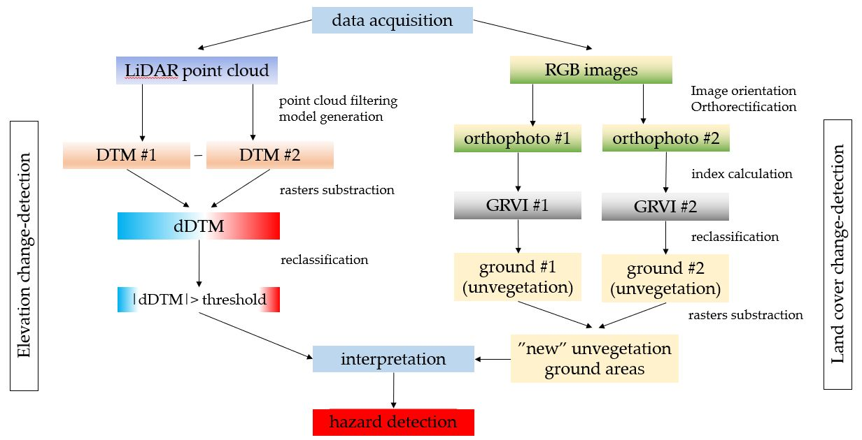
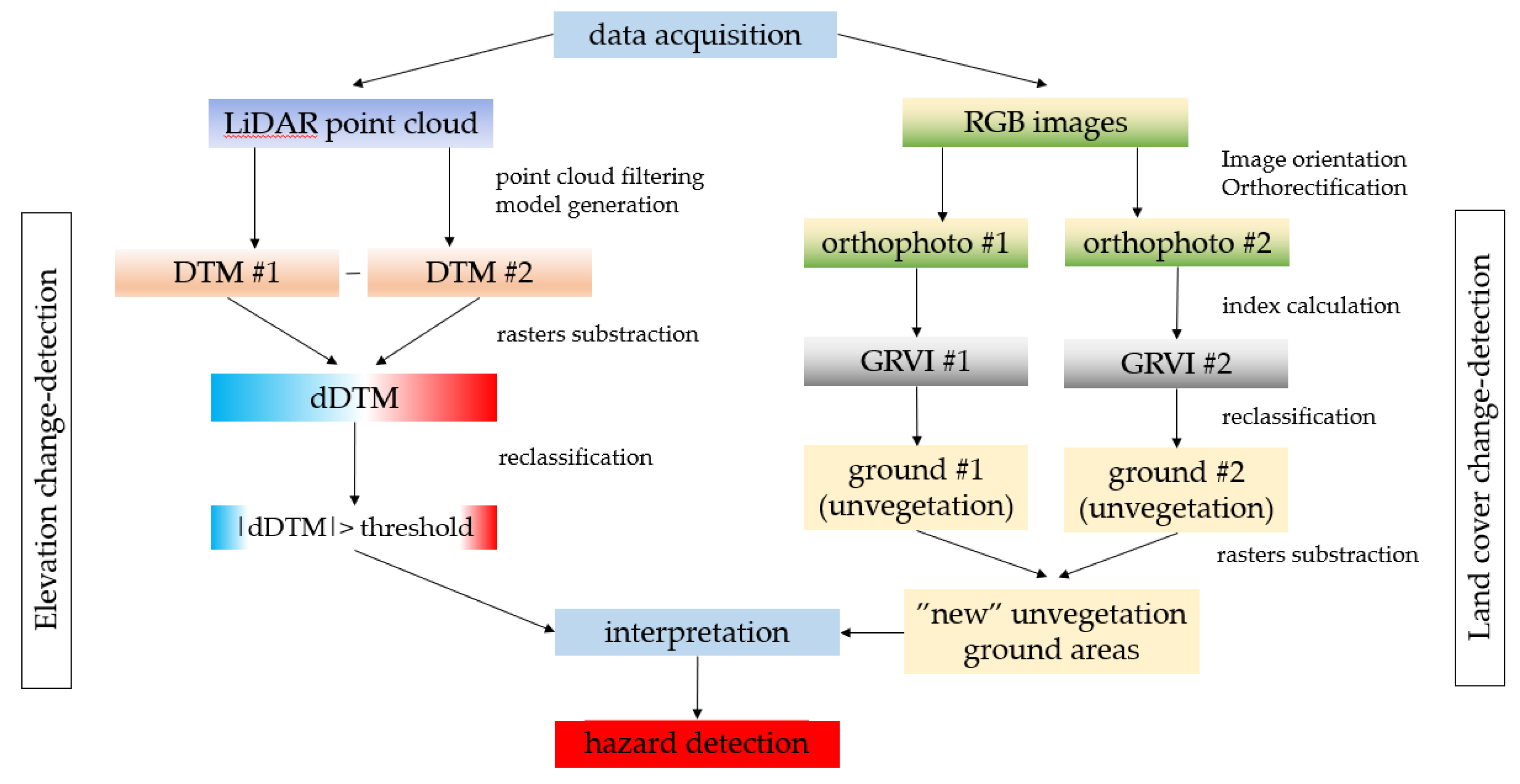
2.1. Description of the Workflow
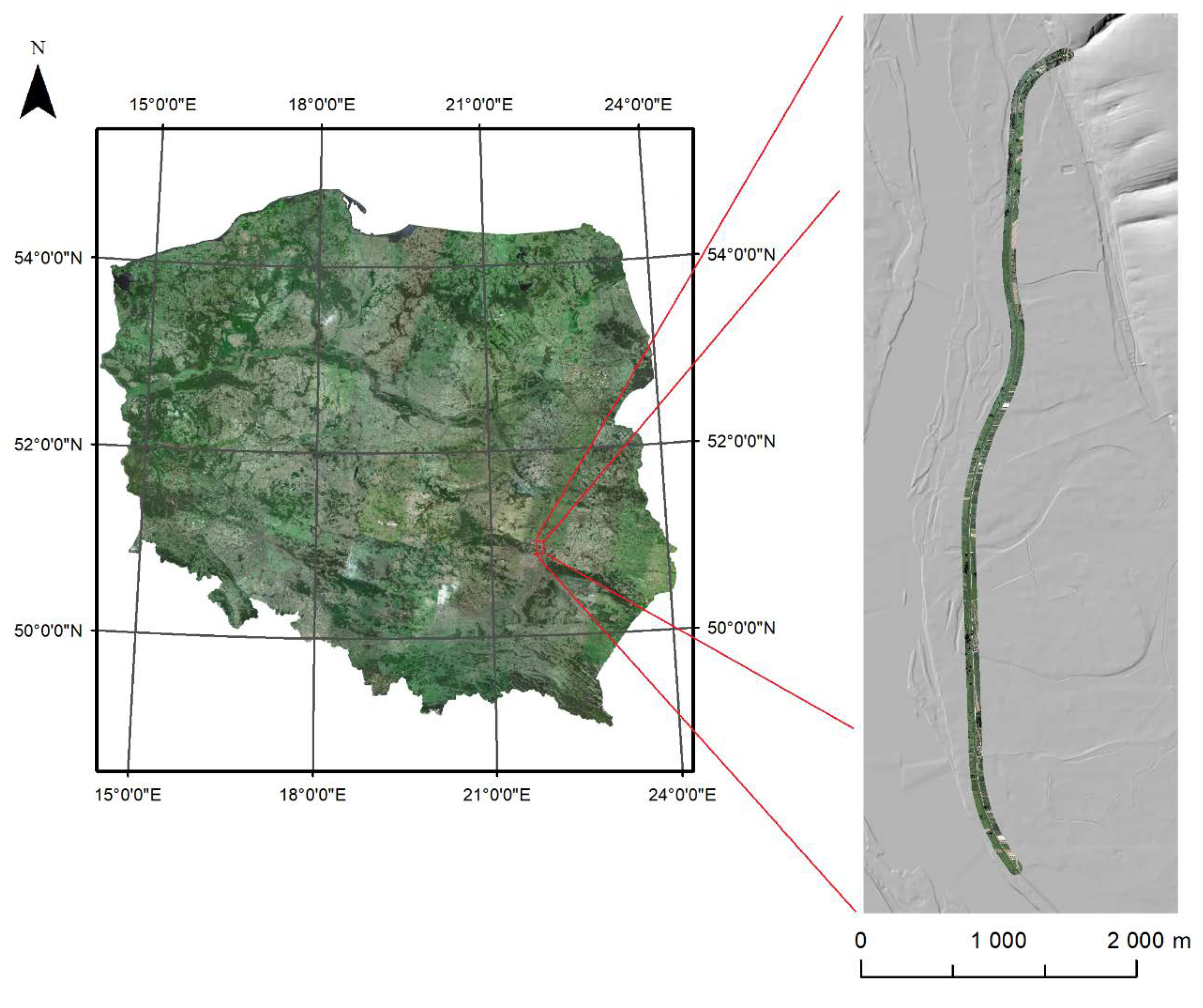
2.2. Description of the Tested Data
3. Results of Change-Detection
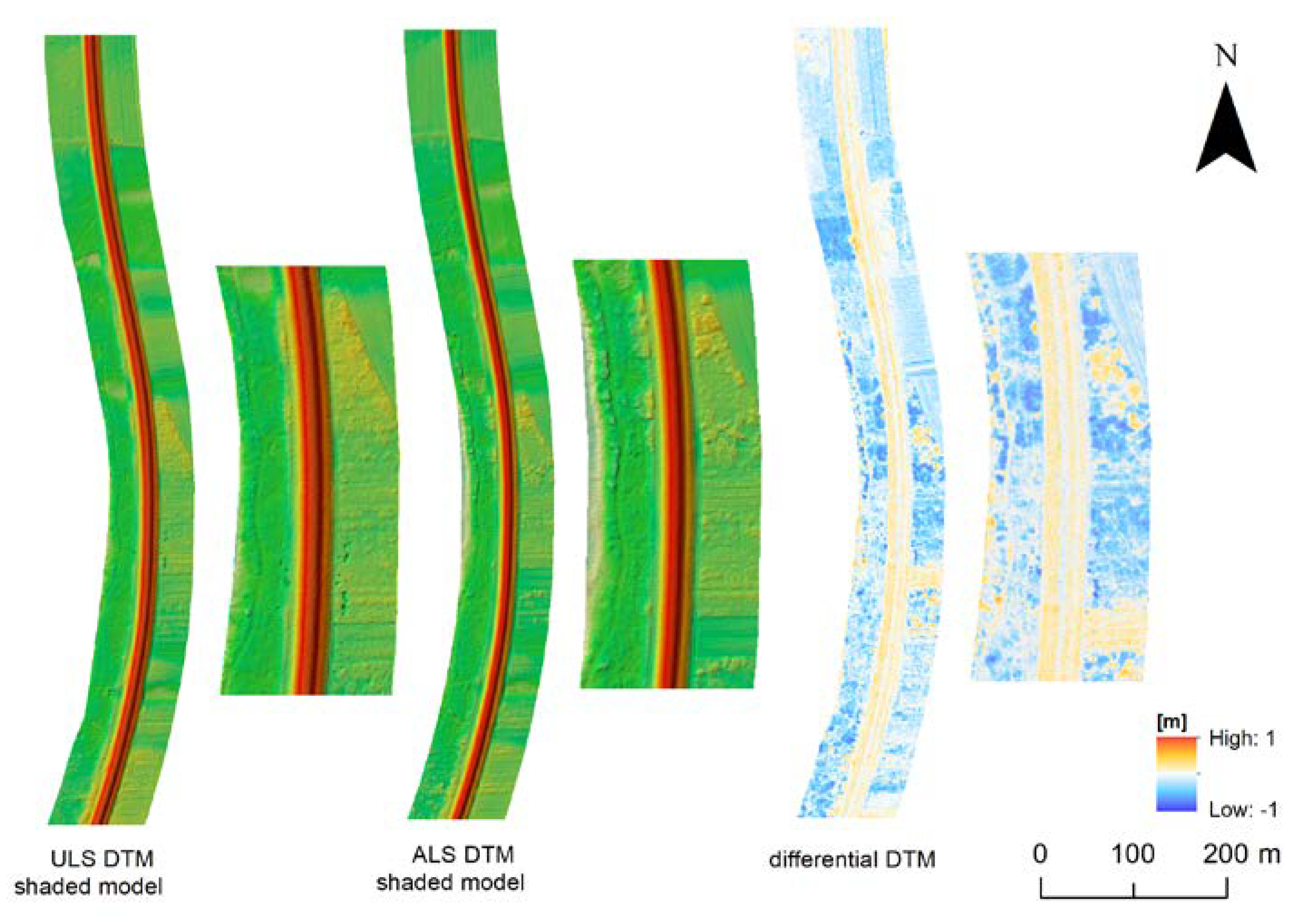
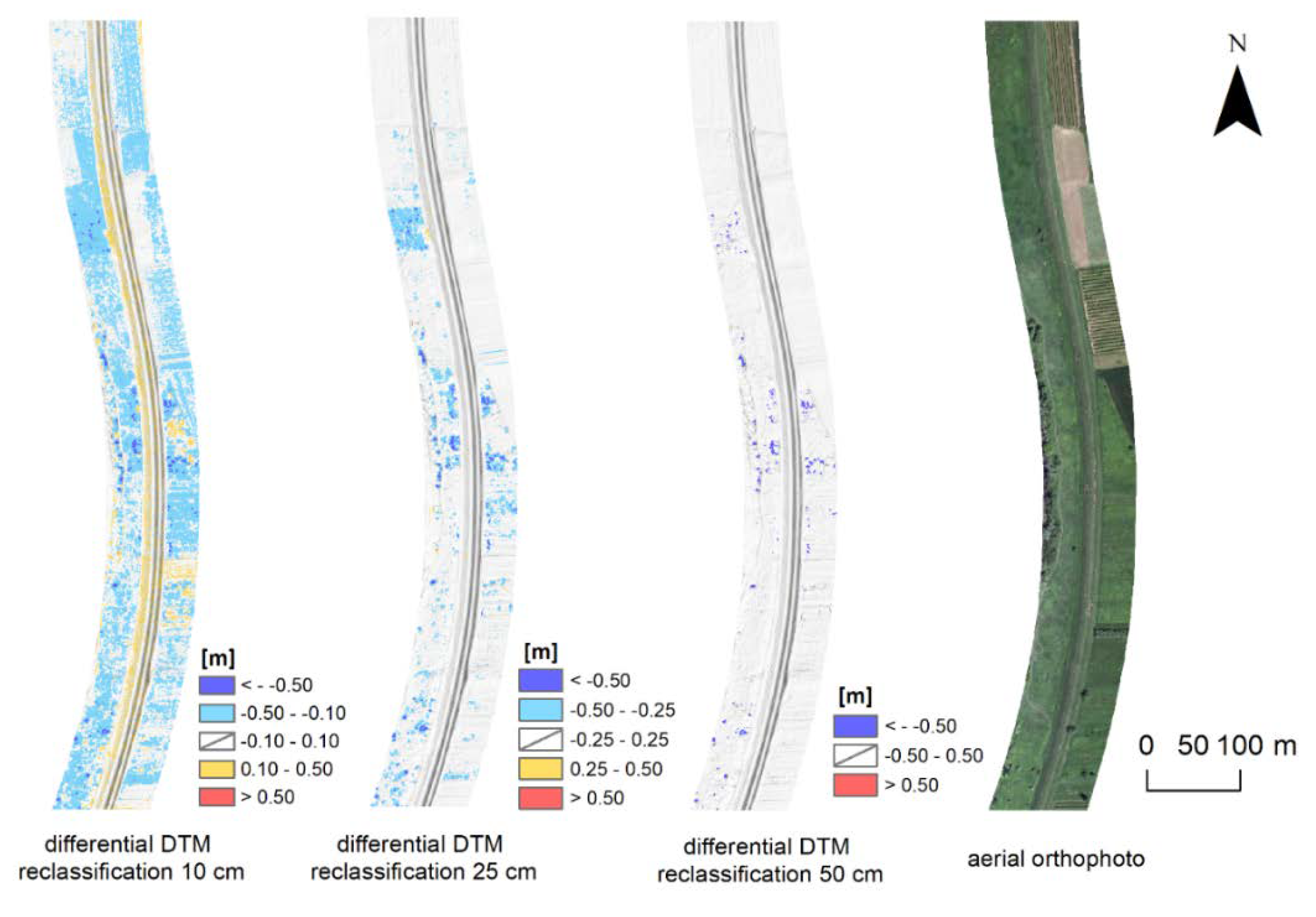
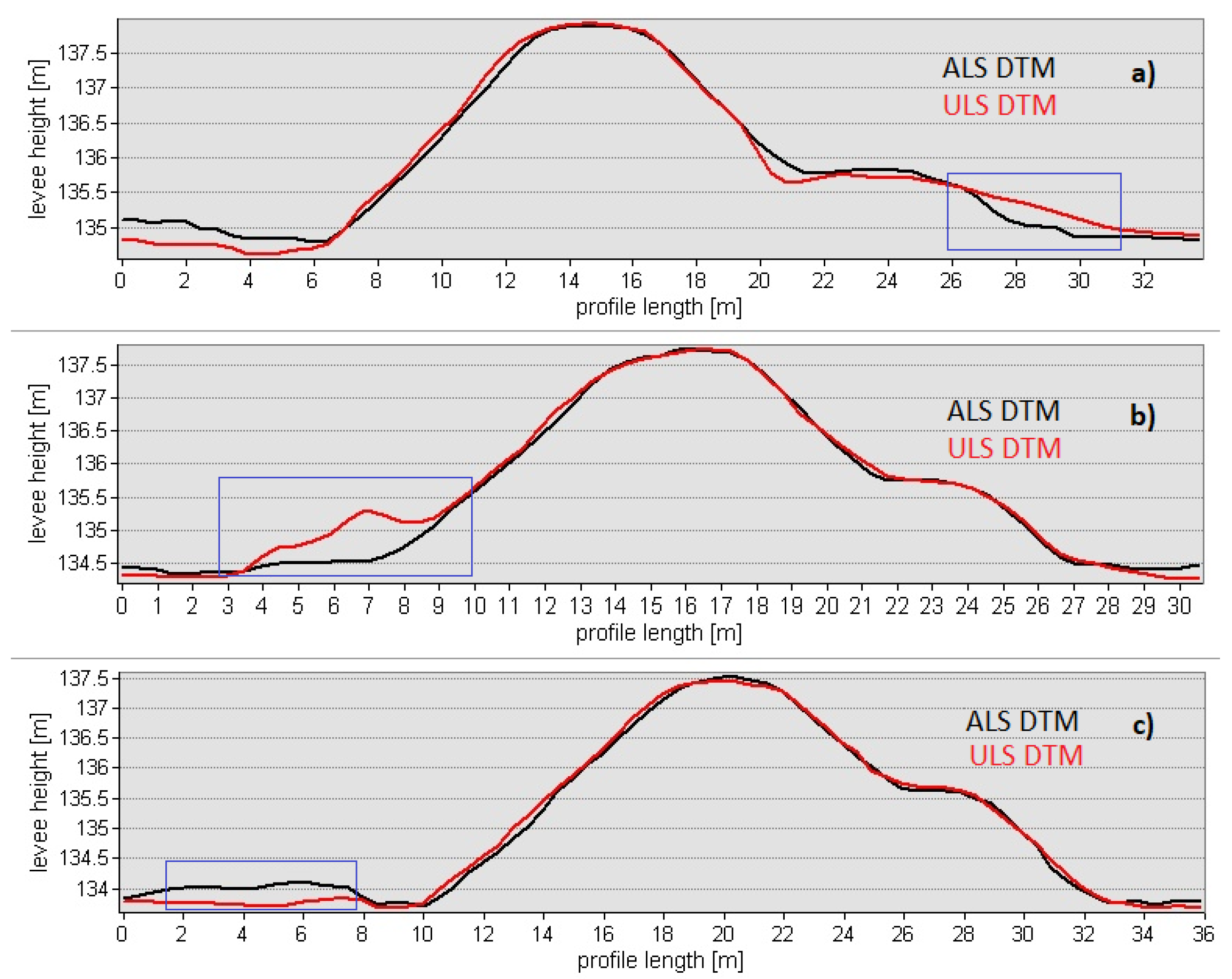
3.1. Elevation Data
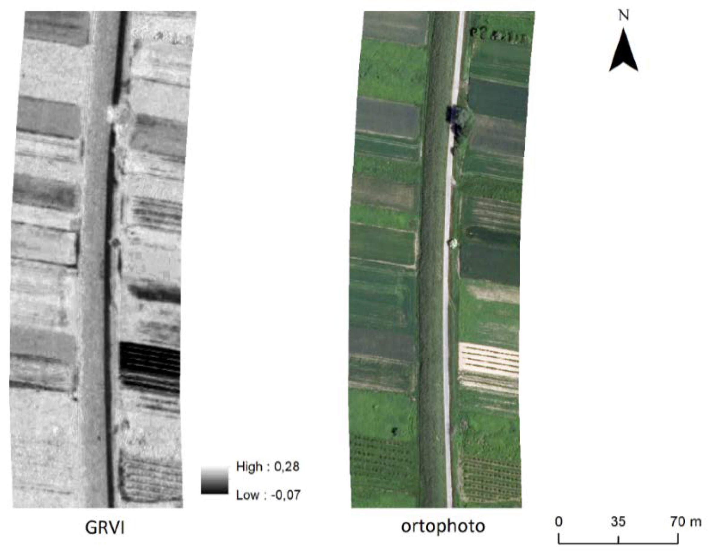
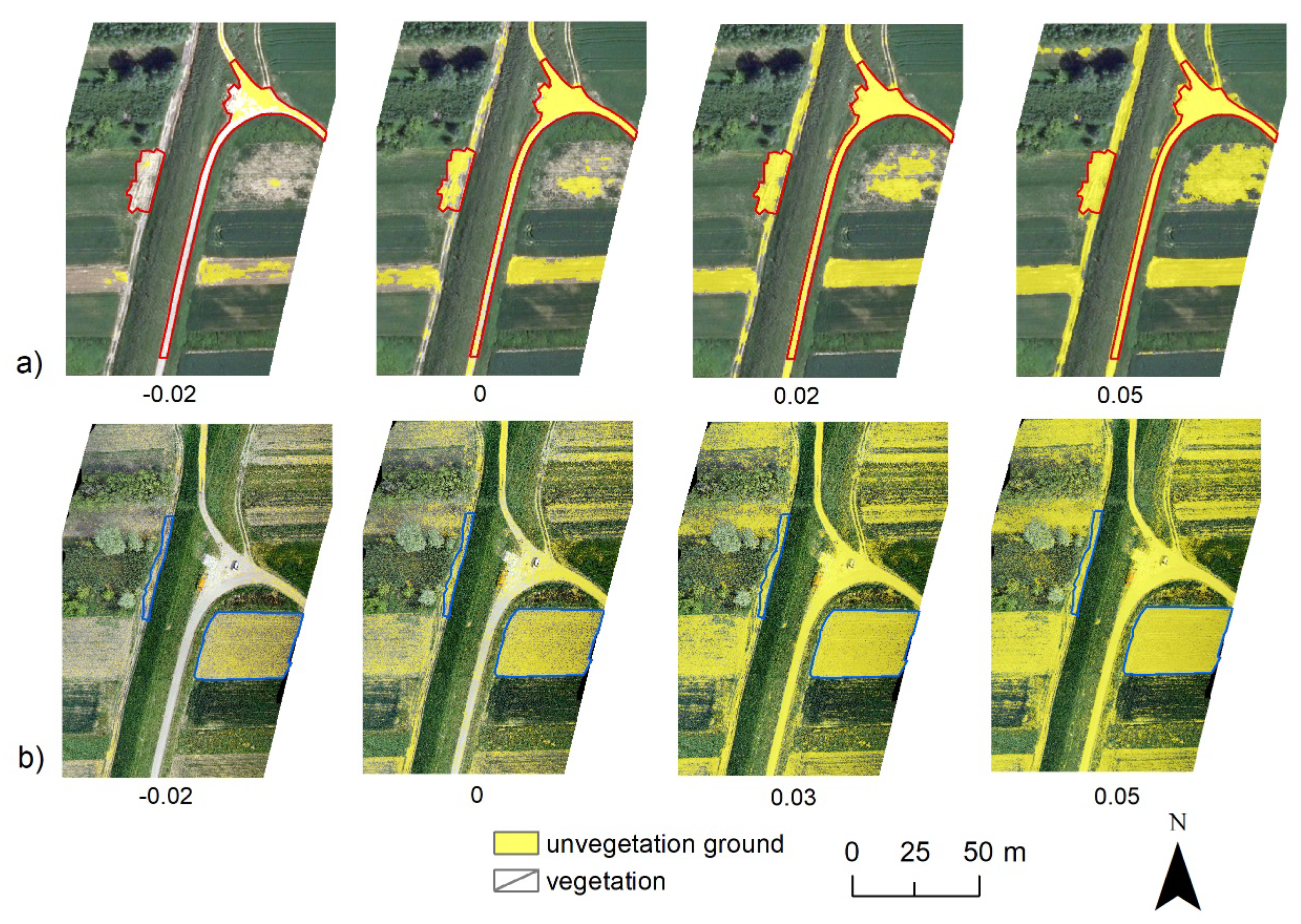
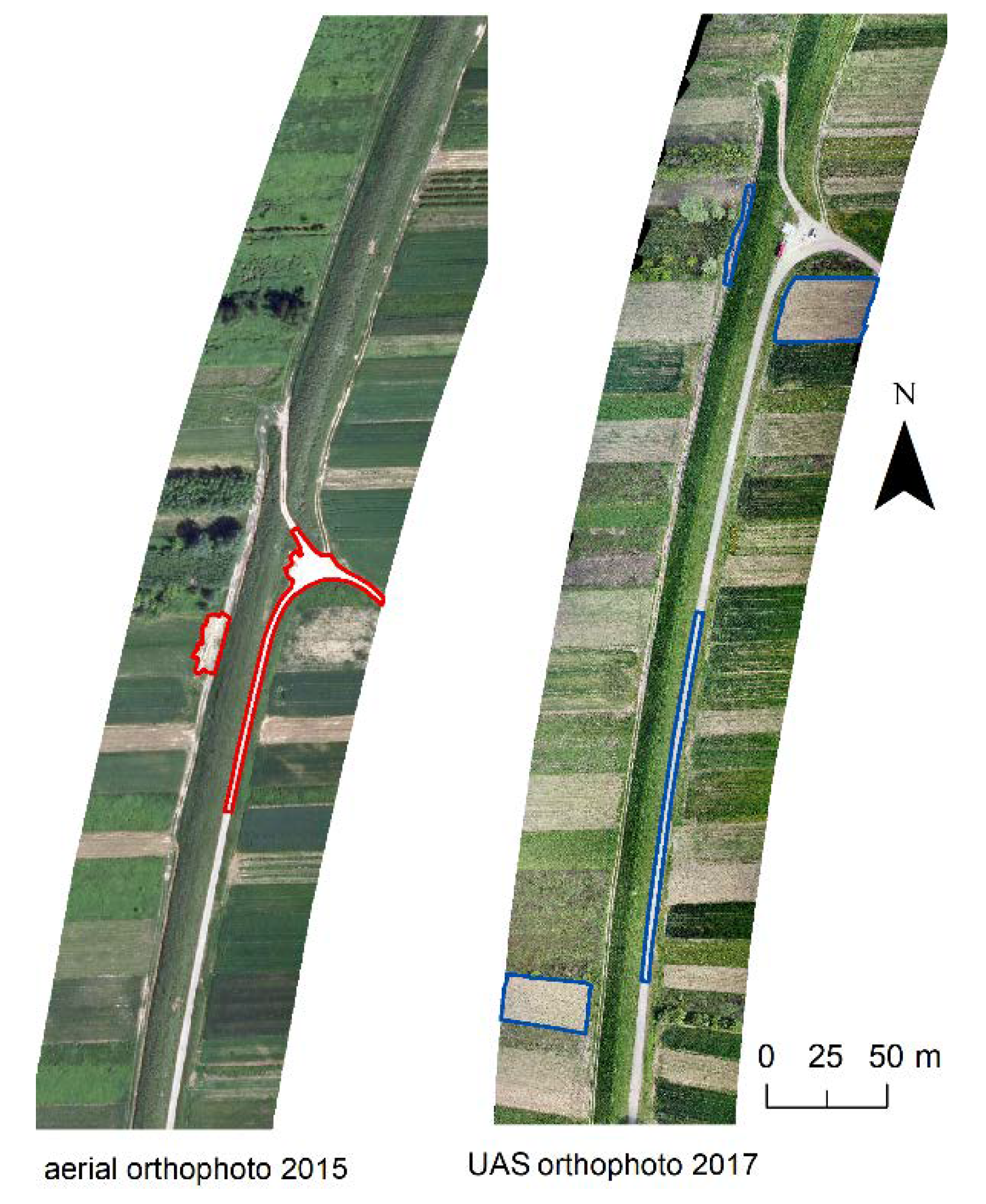
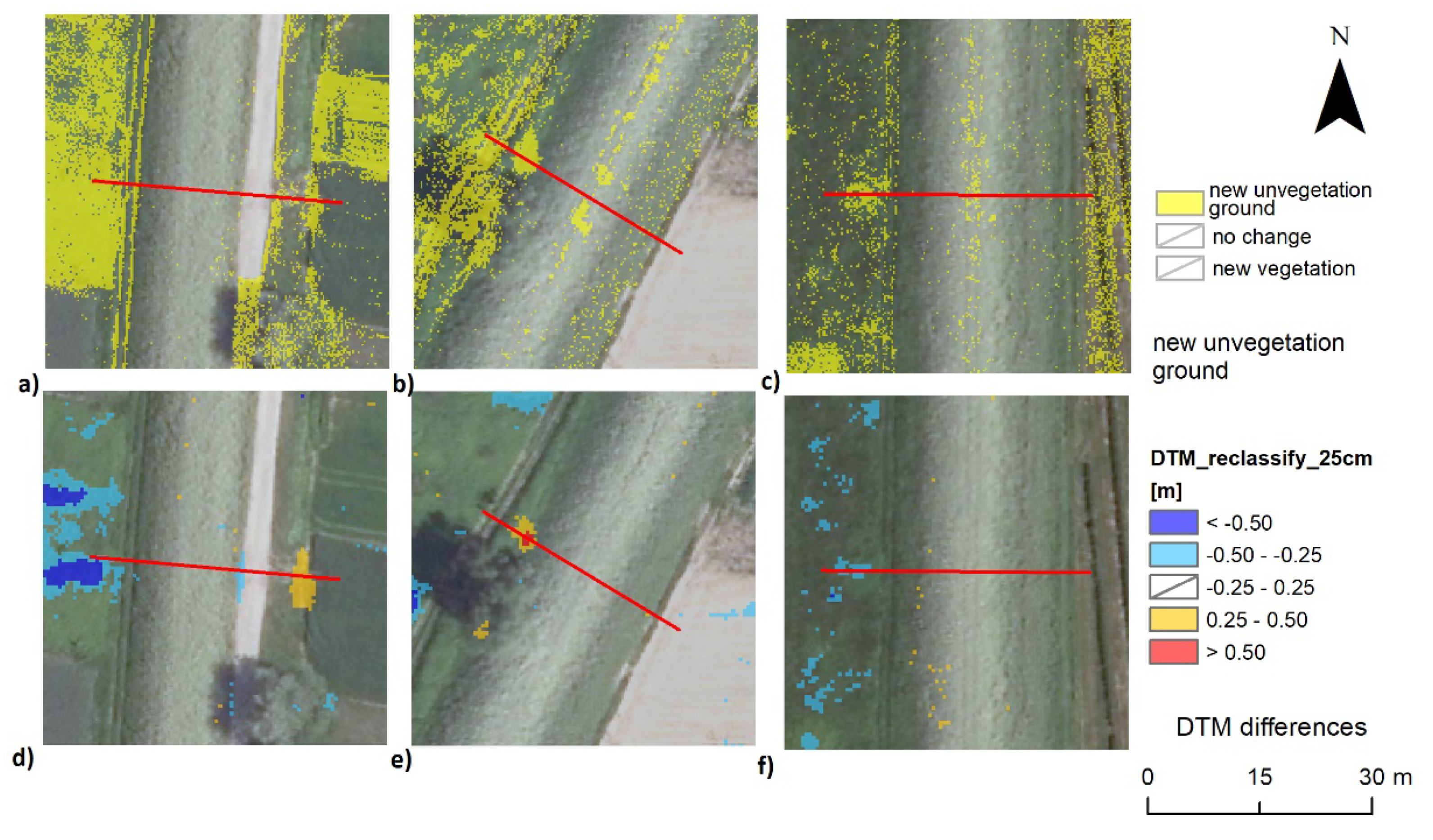
3.2. Optical Data
- ρR—is the reflectance of the visible red on the image
- ρG—is the reflectance of the visible green on the image
3.3. Application of the Results
4. Discussion
5. Conclusions
Author Contributions
Funding
Acknowledgments
Conflicts of Interest
References
- Tralli, D.M.; Blom, R.G.; Zlotnicki, V.; Donnellan, A.; Evans, D.L. Satellite remote sensing of earthquake, volcano, flood, landslide and coastal inundation hazards. ISPRS J. Photogramm. Remote Sens. 2005, 59, 185–198. [Google Scholar] [CrossRef]
- Kussul, N.; Skakun, S.; Shelestov, A.; Lavreniuk, M.; Yailymov, B.; Kussul, O. Regional scale crop mapping using multi-temporal satellite imagery. Int. Arch. Photogramm. Remote Sens. Spat. Inf. Sci. 2015, 40, 45–52. [Google Scholar] [CrossRef] [Green Version]
- Weintrit, B.; Osińska-Skotak, K.; Pilarska, M. Feasibility study of flood risk monitoring based on optical satellite data. Misc. Geogr. 2018, 22, 172–180. [Google Scholar] [CrossRef] [Green Version]
- Yen, B.C. Hydraulics and Effectiveness of Levees for Flood Control. In US–Italy Research Workshop on the Hydrometeorology, Impacts, and Management of Extreme Floods. 1995. Available online: https://www.engr.colostate.edu/ce/facultystaff/salas/us-italy/papers/44yen.pdf (accessed on 14 April 2020).
- Long, G.; Mawdesley, M.J.; Smith, M.; Taha, A. Simulation of airborne LiDAR for the assessment of its role in infrastructure asset monitoring. In Proceedings of the International Conference on Computing in Civil and Building Enginerering; Tizani, W., Ed.; Nottingham University Press: Nottingham, UK, 2010. [Google Scholar]
- Kurczyński, Z.; Bakuła, K. SAFEDAM-zaawansowane technologie wspomagające przeciwdziałanie zagrożeniom związanym z powodziami. Arch. Fotogram. Kartogr. Teledetekcji 2016, 28, 39–52. [Google Scholar]
- Tournadre, V.; Pierrot-Deseilligny, M.; Faure, P.H. UAV photogrammetry to monitor dykes-calibration and comparison to terrestrial lidar. Int. Arch. Photogramm. Remote Sens. Spat. Inf. Sci. 2014, 40, 143. [Google Scholar] [CrossRef] [Green Version]
- Zhou, Y.; Rupnik, E.; Faure, P.H.; Pierrot-Deseilligny, M. GNSS-assisted integrated sensor orientation with sensor pre-calibration for accurate corridor mapping. Sensors 2018, 18, 2783. [Google Scholar] [CrossRef] [Green Version]
- Bakuła, K.; Ostrowski, W.; Szender, M.; Plutecki, W.; Salach, A.; Górski, K. Possibilities for using lidar and photogrammetric data obtained with an unmanned aerial vehicle for levee monitoring. Int. Arch. Photogramm. Remote Sens. Spat. Inf. Sci. 2016, 41, 773–780. [Google Scholar] [CrossRef]
- Baltsavias, E.P. A comparison between photogrammetry and laser scanning. ISPRS J. Photogramm. Remote Sens. 1999, 54, 83–94. [Google Scholar] [CrossRef]
- Zhou, Y. 100% Automatic Metrology with UAV Photogrammetry and Embedded GPS and Its Application in Dike Monitoring. Ph.D. Thesis, Université Paris-Est, Paris, France, 2019. [Google Scholar]
- Berni, J.A.J.; Zarco-Tejada, P.J.; Suárez, L.; González-Dugo, V.; Fereres, E. Remote sensing of vegetation from UAV platforms using lightweight multispectral and thermal imaging sensors. Int. Arch. Photogramm. Remote Sens. Spat. Inform. Sci. 2009, 38, 6. [Google Scholar]
- Hunt, E.R.; Hively, W.D.; Fujikawa, S.; Linden, D.; Daughtry, C.S.; McCarty, G. Acquisition of NIR-green-blue digital photographs from unmanned aircraft for crop monitoring. Remote Sens. 2010, 2, 290–305. [Google Scholar] [CrossRef] [Green Version]
- Torres-Sánchez, J.; López-Granados, F.; Peña, J.M. An automatic object-based method for optimal thresholding in UAV images: Application for vegetation detection in herbaceous crops. Comput. Electron. Agric. 2015, 114, 43–52. [Google Scholar] [CrossRef]
- D’Oleire-Oltmanns, S.; Marzolff, I.; Peter, K.D.; Ries, J.B. Unmanned aerial vehicle (UAV) for monitoring soil erosion in Morocco. Remote Sens. 2012, 4, 3390–3461. [Google Scholar] [CrossRef] [Green Version]
- Torres-Sánchez, J.; Peña, J.M.; de Castro, A.I.; López-Granados, F. Multi-temporal mapping of the vegetation fraction in early-season wheat fields using images from UAV. Comput. Electron. Agric. 2014, 103, 104–113. [Google Scholar] [CrossRef]
- Eltner, A.; Baumgart, P.; Maas, H.; Faust, D. Multi-temporal UAV data for automatic measurement of rill and interrill erosion on loess soil. Earth Surf. Process. Landforms 2015, 40, 741–755. [Google Scholar] [CrossRef]
- Bakuła, K.; Ostrowski, W.; Pilarska, M.; Szender, M.; Kurczyński, Z. Evaluation and calibration of fixed-wing multisensor uav mobile mapping system: Improved results. Int. Arch. Photogramm. Remote Sens. Spat. Inf. Sci. 2019, 42, 189–195. [Google Scholar] [CrossRef] [Green Version]
- Salach, A.; Bakuła, K.; Pilarska, M.; Ostrowski, W.; Górski, K.; Kurczyński, Z. Accuracy Assessment of Point Clouds from LiDAR and Dense Image Matching Acquired Using the UAV Platform for DTM Creation. ISPRS Int. J. Geo-Inf. 2018, 7, 342. [Google Scholar] [CrossRef] [Green Version]
- Wallace, L.; Lucieer, A.; Malenovskỳ, Z.; Turner, D.; Vopěnka, P. Assessment of forest structure using two UAV techniques: A comparison of airborne laser scanning and structure from motion (SfM) point clouds. Forests 2016, 7, 62. [Google Scholar] [CrossRef] [Green Version]
- Weintrit, B.; Bakuła, K.; Jędryka, M.; Bijak, W.; Ostrowski, W.; Wziątek, D.Z.; Ankowski, A.; Kurczyński, Z. Emergency rescue management supported by UAV remote sensing data. Int. Arch. Photogramm. Remote Sens. Spat. Inf. Sci. 2018, 42, 563–567. [Google Scholar] [CrossRef] [Green Version]
- Kurczyński, Z.; Bakuła, K. The selection of aerial laser scanning parameters for countrywide digital elevation model creation. In Proceedings of the 13th SGEM GeoConference of Informatics, Geoinformatics and Remote Sensing, Albena, Bulgaria, 16–22 June 2013; Volume 2, pp. 695–702. [Google Scholar]
- Dewitte, O.; Jasselette, J.C.; Cornet, Y.; Van Den Eeckhaut, M.; Collignon, A.; Poesen, J.; Demoulin, A. Tracking landslide displacements by multi-temporal DTMs: A combined aerial stereophotogrammetric and LIDAR approach in western Belgium. Eng. Geol. 2008, 99, 11–22. [Google Scholar] [CrossRef]
- Allemand, P.; Delacourt, C.; Gasperini, D.; Kasperski, J.; Pothérat, P. Thirty Years of Evolution of the Sedrun Landslide (Swisserland) from Multitemporal Orthorectified Aerial Images, Differential Digital Terrain Models and Field Data. Int. J. Remote Sens. Appl. 2011, 1, 30–36. [Google Scholar]
- Zieher, T.; Perzl, F.; Rössel, M.; Rutzinger, M.; Meißl, G.; Markart, G.; Geitner, C. A multi-annual landslide inventory for the assessment of shallow landslide susceptibility–Two test cases in Vorarlberg, Austria. Geomorphology 2016, 259, 40–54. [Google Scholar] [CrossRef]
- Motohka, T.; Nasahara, K.N.; Oguma, H.; Tsuchida, S. Applicability of green-red vegetation index for remote sensing of vegetation phenology. Remote Sens. 2010, 2, 2369–2387. [Google Scholar] [CrossRef] [Green Version]
- Nagai, S.; Saitoh, T.M.; Kobayashi, H.; Ishihara, M.; Suzuki, R.; Motohka, T.; Nasahara, K.N.; Muraoka, H. In situ examination of the relationship between various vegetation indices and canopy phenology in an evergreen coniferous forest, Japan. Int. J. Remote Sens. 2012, 33, 6202–6214. [Google Scholar] [CrossRef]
- Bendig, J.; Yu, K.; Aasen, H.; Bolten, A.; Bennertz, S.; Broscheit, J.; Gnyp, M.L.; Bareth, G. Combining UAV-based plant height from crop surface models, visible, and near infrared vegetation indices for biomass monitoring in barley. Int. J. Appl. Earth Obs. Geoinf. 2015, 39, 79–87. [Google Scholar] [CrossRef]


| Dataset | Acquisition Date | Resolution/ Density | Accuracy | Sensor |
|---|---|---|---|---|
| aerial orthophoto | June 2015 | 0.25 m | 0.50 m horizontal | UltraCam-Xp |
| UAS orthophoto | May 2017 | 0.10 m | 0.10 m horizontal | Sony Alpha 6000 |
| aerial LiDAR | October 2011 | 4 points/m2 | 0.15 m vertical 0.40 m horizontal | N/A |
| ULS | May 2017 | 180 points/m2 | 0.10 m vertical 0.20 m horizontal | YellowScan Surveyor |
| GRVI Threshold | Orthophoto from Aerial Images | Orthophoto from UAS Images | ||||
|---|---|---|---|---|---|---|
| No. of px (resol. 0.25 m) | Area (m2) | Area (%) | No. of px (resol. 0.10 m) | Area (m2) | Area (%) | |
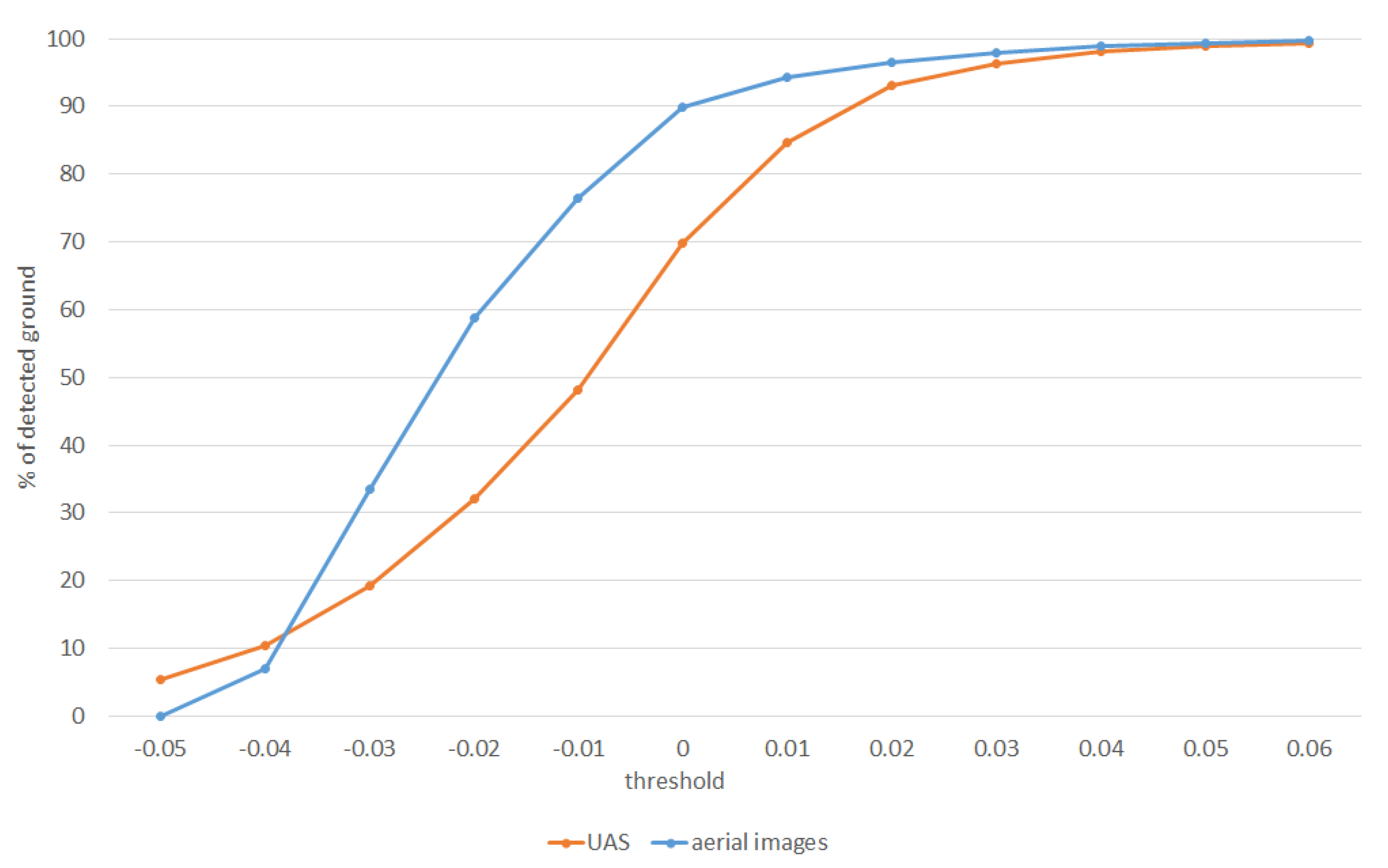
| 0.06 | 57,165 | 3572.8 | 99.8 | 256,321 | 2563.2 | 99.3 |
| 0.05 | 56,964 | 3560.2 | 99.4 | 255,051 | 2550.5 | 98.9 |
| 0.04 | 56,624 | 3539.0 | 98.8 | 252,990 | 2529.9 | 98.1 |
| 0.03 | 56,111 | 3506.9 | 97.9 | 248,710 | 2487.1 | 96.4 |
| 0.02 | 55,316 | 3457.2 | 96.5 | 240,165 | 2401.7 | 93.1 |
| 0.01 | 54,038 | 3377.4 | 94.3 | 218,384 | 2183.8 | 84.6 |
| 0.00 | 51,523 | 3220.2 | 89.9 | 179,917 | 1799.2 | 69.7 |
| −0.01 | 43,762 | 2735.1 | 76.4 | 124,356 | 1243.6 | 48.2 |
| −0.02 | 33,653 | 2103.3 | 58.7 | 82,727 | 827.3 | 32.1 |
| −0.03 | 19,134 | 1195.9 | 33.4 | 49,612 | 496.1 | 19.2 |
| −0.04 | 4045 | 252.8 | 7.1 | 27,018 | 270.2 | 10.5 |
| −0.05 | 17 | 1.1 | 0.0 | 14,019 | 140.2 | 5.4 |
© 2020 by the authors. Licensee MDPI, Basel, Switzerland. This article is an open access article distributed under the terms and conditions of the Creative Commons Attribution (CC BY) license (http://creativecommons.org/licenses/by/4.0/).
Share and Cite
Bakuła, K.; Pilarska, M.; Salach, A.; Kurczyński, Z. Detection of Levee Damage Based on UAS Data—Optical Imagery and LiDAR Point Clouds. ISPRS Int. J. Geo-Inf. 2020, 9, 248. https://0-doi-org.brum.beds.ac.uk/10.3390/ijgi9040248
Bakuła K, Pilarska M, Salach A, Kurczyński Z. Detection of Levee Damage Based on UAS Data—Optical Imagery and LiDAR Point Clouds. ISPRS International Journal of Geo-Information. 2020; 9(4):248. https://0-doi-org.brum.beds.ac.uk/10.3390/ijgi9040248
Chicago/Turabian StyleBakuła, Krzysztof, Magdalena Pilarska, Adam Salach, and Zdzisław Kurczyński. 2020. "Detection of Levee Damage Based on UAS Data—Optical Imagery and LiDAR Point Clouds" ISPRS International Journal of Geo-Information 9, no. 4: 248. https://0-doi-org.brum.beds.ac.uk/10.3390/ijgi9040248