High-Resolution Remote Sensing Image Integrity Authentication Method Considering Both Global and Local Features

Abstract

Content integrity of high-resolution remote sensing (HRRS) images is the premise of its usability. Existing HRRS image integrity authentication methods are mostly binary decision-making processes, which cannot provide a further interpretable information (e.g., tamper localization, tamper type determination). Due to this reason, a robust HRRS images integrity authentication algorithm using perceptual hashing technology considering both global and local features is proposed in this paper. It extracts global features by the efficient recognition ability of Zernike moments to texture information. Meanwhile, Features from Accelerated Segment Test (FAST) key points are applied to local features construction and tamper localization. By applying the concept of multi-feature combination to the integrity authentication of HRRS images, the authentication process is more convincing in comparison to existing algorithms. Furthermore, an interpretable authentication result can be given. The experimental results show that the algorithm proposed in this paper is highly robust to the content retention operation, has a strong sensitivity to the content changing operations, and the result of tampering localization is more precise comparing with existing algorithms.

1. Introduction

As an important carrier of geospatial information, high-resolution remote sensing (HRRS) images have been widely used in military exploration [1], resource monitoring [2], disaster assessment [3], high-precision navigation [4] and many other fields. Recently, with the widespread application of remote sensing image processing software and the rapid development of information sharing technology, the utilization rate of HRRS images is gradually increasing. Meanwhile, it also has more risk of being maliciously tampered than ever. If the content integrity of HRRS images is questioned, their use value will be greatly reduced [5]. Therefore, how to identify the content integrity of HRRS images is an important issue.

Data integrity refers to the fact that the content of data does not change during transmission and application [6]. Many scholars have studied the integrity authentication methods of remote sensing images, and these methods are mostly based on digital signature technology [7], digital watermark technology [8], and perceptual hashing technology [9]. Generally, digital signature means that the data sender describes the original data as a unique string digest through MD5, SHA-1 and other algorithms [10], and the data receiver implements integrity authentication through the digest match. This type of method is extremely sensitive to bit-level changes (a 1-bit change in data is considered tampering), which is only suitable for precise authentication such as text information and is not robust to content retention operations. In essence, it only tests the consistency of data in binary representation without considering the consistency of data content.

Digital watermarking usually embeds the identity information into the original data, and the data receiver extracts the identification information through the extraction algorithms. The integrity of this identification information represents the integrity of the data. These methods usually take the content characteristics of data into consideration, and some of which can achieve tamper localization. Li [11] proposed a remote sensing fragile watermarking algorithm based on the improved Least Significant Bit (LSB) technology, which improved the security and computational efficiency of the traditional fragile watermark authentication algorithms. Jordi [12] proposed a semi-fragile watermark integrity authentication scheme for multi-band remote sensing images. The tree structure vector quantization method was applied to the generation of identification information, which is robust to JPEG compression, gaussian noise, etc. Zhang [13] proposed a remote sensing fragile watermarking algorithm for content reconstruction by using the brief representation of data, and the remote sensing image of the tampered area can be recovered approximately. There are also other scholars studying the remote sensing image integrity authentication method based on digital watermarking technology [14,15,16]. However, the integrity authentication algorithm based on digital watermarking generally has the following shortcomings:

• The process of watermark embedding is a modification of the original data, which is not allowed in some fields, especially in the high-fidelity field.
• Watermark-based authentication is essentially a carrier-based authentication. If format conversion is applied to the data without modifying the content, the watermark information may also change greatly.

Perceptual hashing technology can provide new solutions to the above problems. Perceptual hashing is a method to map multimedia data into hash sequence, which is robust to content retention operations and sensitive to content tampering operations [17]. It is widely used in information retrieval [18,19,20], data authentication [21,22,23], copy detection [24,25] and other fields. The realization of perceptual hash is as follows: The data sender generates the hash sequence by feature extraction and feature compression, and the data receiver verifies the integrity by comparing the similarity of the hash sequence. Compared with digital signature-based methods, the most significant feature of perceptual hashing is that it is perceptually robust, which means that after performing content retention operations (such as format conversion and watermark embedding) on the image, the hash sequence does not change significantly. Compared with digital watermarking, perceptual hashing does not need to embed any information into the data, and the hash sequence is highly dependent on the content of the data, which overcomes the disadvantage that digital watermarking relies too much on the information carrier. Some perceptual hashing algorithms of remote sensing images has been carried out and applied to image retrieval [26] and authentication [27,28,29]. Reference [27] used the pyramid model constructed a multi-scale HRRS image authentication model. Reference [28] used Canny operator for edge detection, combined DWT and Gabor filter to construct a perceptual hash integrity authentication method for HRRS images. In Reference [29], A U-net network was used to improve the method in [28]. The edge features extracted by Canny operator were more refined through the independent learning of U-net network, but the learning results of this algorithm needed a lot of manual correction.

However, the integrity authentication algorithm of HRRS images still has the following problems:

• Most of the existing HRRS perceptual hashing algorithms are based on one feature for authentication. Remote sensing images have the characteristics of data magnanimity, and generally there is no clear subject information, so the authentication results based on a single feature are not convincing.
• Existing algorithms are essentially a process of binary decision-making; that is, there are only two results: to pass the integrity authentication and to not pass the integrity authentication. A further interpretable information cannot be given by these algorithms.

To overcome these problems, a HRRS perceptual hashing algorithm combine Zernike moments and FAST feature descriptors is proposed in this paper. Additionally, the characteristics of HRRS images with high accuracy and large data size is fully considered. While improving the robustness and tampering recognition capabilities, this algorithm can also provide a further interpretable evidence for the integrity authentication of HRRS images.

The rest of this paper is organized as follows: Section 2 outlines the progress of relevant research. Section 3 describes the method we proposed. Section 4 analyzes and discusses the experimental results. And, Section 5 gives the conclusion of this paper.

2. Related Works

2.1. Perceptual Hashing

Perceptual hashing is rooted from digital signature technology. As mentioned above, it can map multimedia data (such as images and videos) into a sequence of summaries of a certain length, that is, the content information of multimedia data can be represented with as little information as possible.

HRRS images have similarities with digital images in data organization, so the successful experiences of image perceptual hash cannot be ignored. For digital images, the procedure of perceptual hashing is shown in Figure 1, which consists of hash generation and hash comparison [30]. Figure 1a shows the procedure of hash generation, which consists of feature extraction and feature compression: the two-dimensional image is mapped to a one-dimensional array, and the robustness information is extracted to form the hash sequence. Figure 1b shows the procedure of hash comparison: the hash sequence is transmitted by a reliable channel, and the image may be tampered during the transmission. The receiver uses the same algorithm as the sender to generate a hash sequence Hash2 of the image to be authenticated and performs hash comparison with the original hash Hash1 to generate the authentication result.

Feature extraction is the key of the perceptual hashing algorithm. The feature extraction methods are mainly based on edge detection [28,29], key point detection [31,32], DCT (Discrete Cosine Transform) [33,34], DWT (Discrete Wavelet Transform) [35,36] and other feature extraction methods. As a specific application of perceptual hash in HRRS image, it should have the characteristics of image perceptual hash:

• One-way: hash sequence can be generated from the image, but the image information cannot be generated from hash sequence.
• Collision resistance: different images generate completely different hash sequence.
• Perceptual robustness: hash sequence does not change significantly after content retention operations.
• Tampering sensitivity: after content tampering operations, the value of the hash sequence can change greatly.

2.2. High-Resolution Remote Sensing Image

The main feature of HRRS images is the strong resolution of ground objects. Currently, the resolution of commonly used commercial HRRS images has reached the sub-meter level. For example, the resolution of the WorldView-3 satellite has reached 0.3 m, and the resolution of the JL-1 commercial satellite developed in China has reached 0.72 m. Compared with low-resolution or medium-low resolution satellite data, HRRS images can show more detailed information of ground objects.

HRRS images require high measurement accuracy, while image perception hashing algorithm cannot meet the requirements of HRRS images. The interpretation of HRRS images content has diversity and ambiguity, which increases the difficulty of extracting HRRS images content features by the perceptual hash algorithm. Additionally, there is usually no unique subject information in a remote sensing image, which increases the uncertainty of HRRS images perceptual feature extraction. In addition, due to the development of data sharing technology, the authentication process should be as fast as possible. However, the computational efficiency of large size images is generally not considered in image perception hashing algorithms.

Therefore, while satisfying the above image perceptual hash characteristics, Hash algorithms for HRRS images should also meet the following characteristics:

• Micro tamper identification capability: by setting the protection level, micro tamper higher than the protection level can be detected.
• Tampering localization capability: the remote sensing image size is usually large, and good algorithms should be able to provide specific tampering locations.
• The computation efficiency and authentication accuracy should be balanced.

In addition, in order to meet the characteristics of the above HRRS images, some targeted designs are needed. The design of this algorithm for remote sensing data includes but is not limited to:

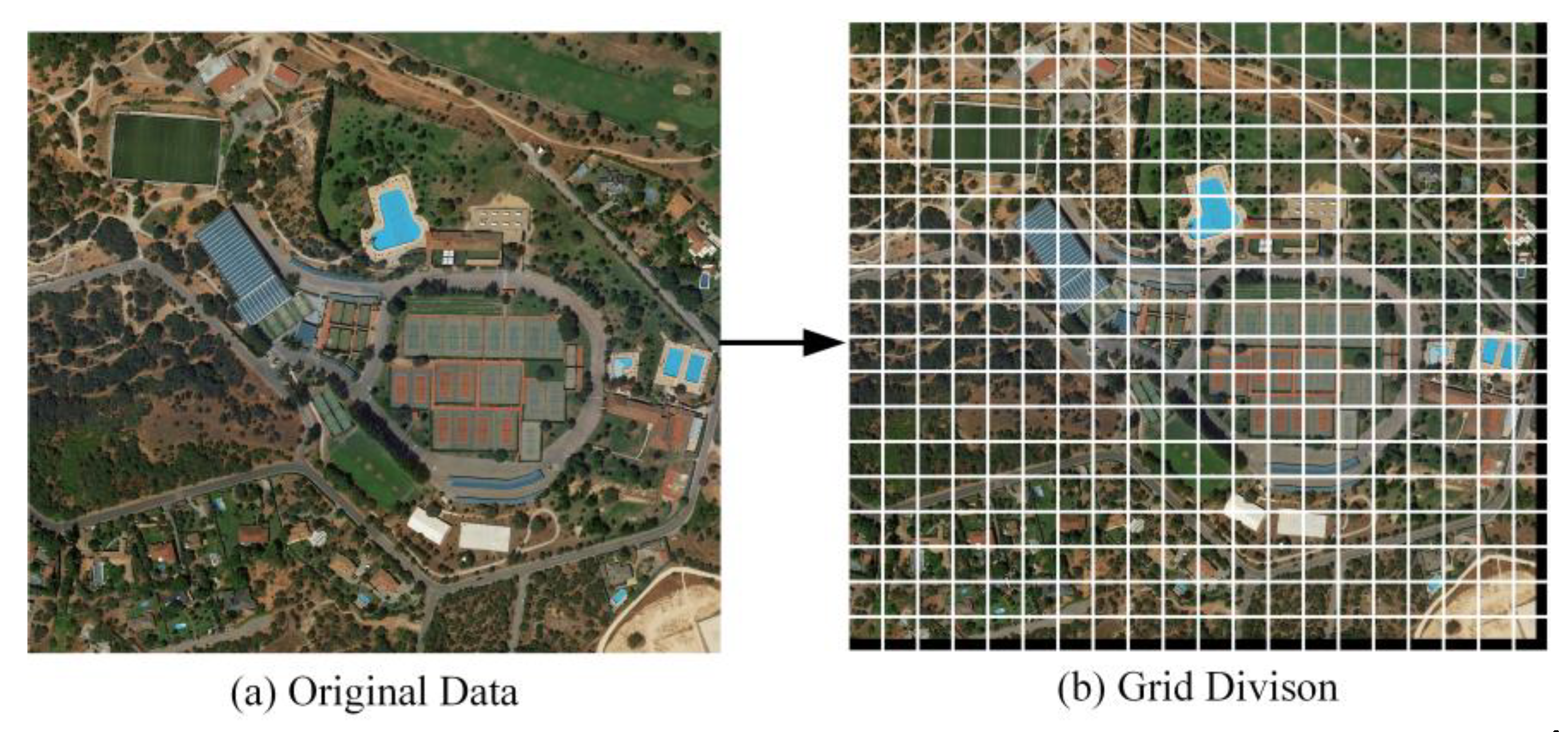
• The method of grid division is introduced to extract the data features of HRRS images in a more detailed way comparing with existing image perceptual hashing algorithms, which satisfied the accuracy requirements of HRRS images.
• A comprehensive description of the image content is made by combining global features and local features, which satisfied the diversity and ambiguity characteristics of HRRS images. After all, a single feature can hardly reflect all the main information of an image.
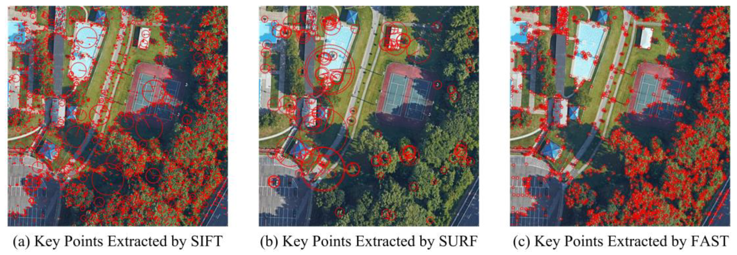
• In consideration of the computational efficiency, the FAST algorithm is adopted to extract local features. Compared with the existing digital image perceptual hash algorithm, the computational efficiency is greatly improved.

2.3. Zernike Moments

The moment features are invariant in rotation and translation, so it can be used to extract the global image feature. Recently, the moment features used for feature extraction of remote sensing image mainly include histogram moments, Hu moments and Zernike moments, etc. Compared with other methods, Zernike moments shows excellent performance [37] in the tamper detection problem. The Zernike moments was proposed by Zernike [38]. Similar to the features of histogram moments and Hu moments, the features extracted by Zernike moments have the invariance of rotation and translation. Differently, the features extracted by Zernike moments are Mutual independent, with low information redundancy, and insensitive to noise attack. Therefore, the Zernike moment is applied to extract the global features of HRRS images.

For a 2-D digital image $f\left(x,y\right)$, its Zernike moments in order $n$ and repetition $m$ is defined as:

$$Z_{nm}=\frac{n+1}{\pi }{\displaystyle \sum }_x{\displaystyle \sum }_{y}f\left(x,y\right)V_{nm}^{*}\left(\rho ,\theta \right),x^2+y^2\le 1,$$

(1)

where $n,m\in \mathrm{N}$, and $\left|m\right|\le n$, * indicates conjugate complex number; $\left(\rho ,\theta \right)$ are the Polar coordinates that normalize the original image $f\left(x,y\right)$ to (−1,1) and map it to the unit circle, i.e., $\rho =\sqrt{x^2+y^2}$, $\theta =\arctan \left(y/x\right)$; $V_{nm}^{*}\left(\rho ,\theta \right)$ represents the transformation kernel of Zernike moments, which consists of a set of Zernike polynomials expressed as follows:

$$V_{nm}\left(\rho ,\theta \right)=R_{nm}\left(\rho \right)e^{im\theta }.$$

(2)

In this formula, $R_{nm}\left(\rho \right)$ is a Zernike radial polynomial, and $i$ is an imaginary unit.

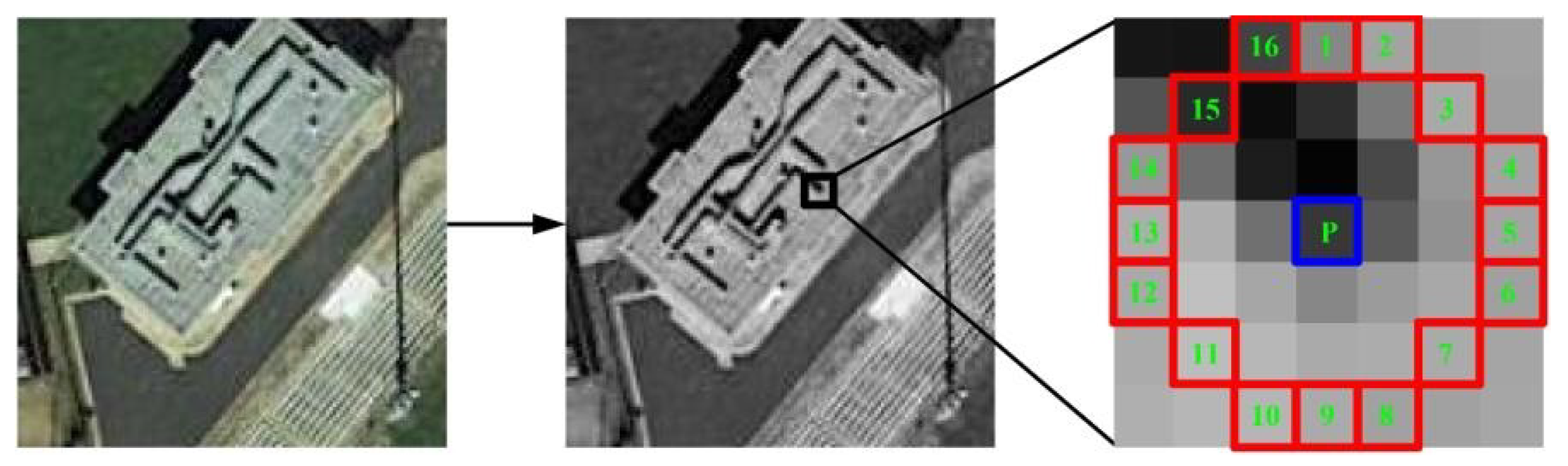
2.4. FAST Key Point Detection

Recently, a series of key point extraction algorithms have been proposed, including Harris [39], Scale-Invariant Feature Transform (SIFT) [40], Speeded Up Robust Features (SURF) [41], Features from Accelerated Segment Test (FAST) [42], etc. Figure 2 shows the results of key points detection results of different methods.

It can be seen that the feature points extracted by various algorithms also have certain similarity in spatial structure. The evaluation of key point extraction algorithm is highly dependent on the practical application scenarios. The SIFT algorithm is characterized by its high rotation invariance and anti-noise capability, which has been applied to digital image integrity authentication [31]. However, the shortcomings of the SIFT algorithm is obvious: its computational complexity is relatively high, especially in HRRS images with a large image size, which may consume a large amount of time. As an improved version of the SIFT algorithm, the SURF algorithm has increased about three times in calculation speed [32], but this improvement is not significant.

The integrity authentication process should be implemented efficiently and conveniently, especially in the era of data sharing. Based on this, the FAST algorithm is applied to local feature extraction in this paper. The FAST key point extraction algorithm was proposed by Rosten [42] in 2011 and is known for its simple calculation process and fast calculation speed. Compared with SIFT and SURF, the FAST algorithm is much faster in key points detection.

2.4.1. Analysis Window Creation

We here present a a brief description of the implementation of the FAST algorithm. First, the color space of the image is converted from RGB to YCbCr. Among them, the Y channel is the brightness component of the image, and it can be used to extract FAST key points. For any pixel $p$ to be detected in the image, draw a Bresenham circle [43] with center $p$ and radius $r$. This circle is consisted of $n$ pixels. Figure 3 shows the schematic diagram when $n=16$ and $r=3$, which is called FAST-16.

2.4.2. Subset Partitioning

For each point $x_n$ in the analysis window mentioned above, its position relative to center $p$ is denoted as $S_{p\to x}$. Then, the following formula is used to divide the subsets:

$$S_{p\to x}=\{\begin{array}{l}d,I_{p\to x}\le I_p-t\\ s,I_p-t\le I_{p\to x}\le I_p+t\\ b,I_{p\to x}+t\le I_{p\to x}\end{array}$$

(3)

In this formula, the threshold $t$ depends on the specific situation. The typical value $t=10$ is chosen in this algorithm. $I$ represents the luminance of points. $“d”$ means that the current point is darker than the central point; “s” means that the current point and the center point have similar luminance; “b” means the current point is lighter than the center. In this way, the pixel set of the whole image can be divided into three subsets.

In practical implementation, in order to improve the speed, the first two pixels on the analysis window are generally detected: If $S_{p\to q_1}=s$ and $S_{p\to q_9}=s$ occur simultaneously, this point is not selected as a candidate key point. Otherwise, continue to detect $S_{p\to q_5}$ and $S_{p\to q_{13}}$. If three of the above four values are “$d$” or “b”, this point will be considered as a candidate key point and continue to calculate the $S_{p\to q_n}$ value of other points in the analysis window. In FAST-16, if the number of points in any subset of “$d$” or “b” is not less than 9, the center $p$ is considered a key point.

2.4.3. Non-Maximal Suppression

Non-maximum suppression is applied to screened key points. Since the above steps can produce many points with similar features, the key points set should be screened to obtain the final feature point set. In essence, FAST is a corner detection algorithm. It is theoretically believed that the sum of the gray difference between the optimal corner and the surrounding pixels should be the largest. Therefore, the response function R is established:

$$R={{\displaystyle \sum }}^{}\frac{\left|I_{p\to q_n}-I_p\right|}{n}$$

(4)

The response R is considered the robustness of the key point. All key points responding in a 3 × 3 neighborhood are calculated according to Equation (4), and then the point with the largest response is retained as the final key point, and other key points in the neighborhood are deleted.

The FAST algorithm will eventually generate a key point set $F$ consisting of n key points:

$$F=\left\{F_1,F_2,\dots ,F_n\right\}$$

(5)

For each key point $F_n$, its composition is as follows:

$$F_n=\left(x,y,R\right)$$

(6)

In this formula, $\left(x,y\right)$ represents the position of the key point; $R$ represents the response value of the key point.

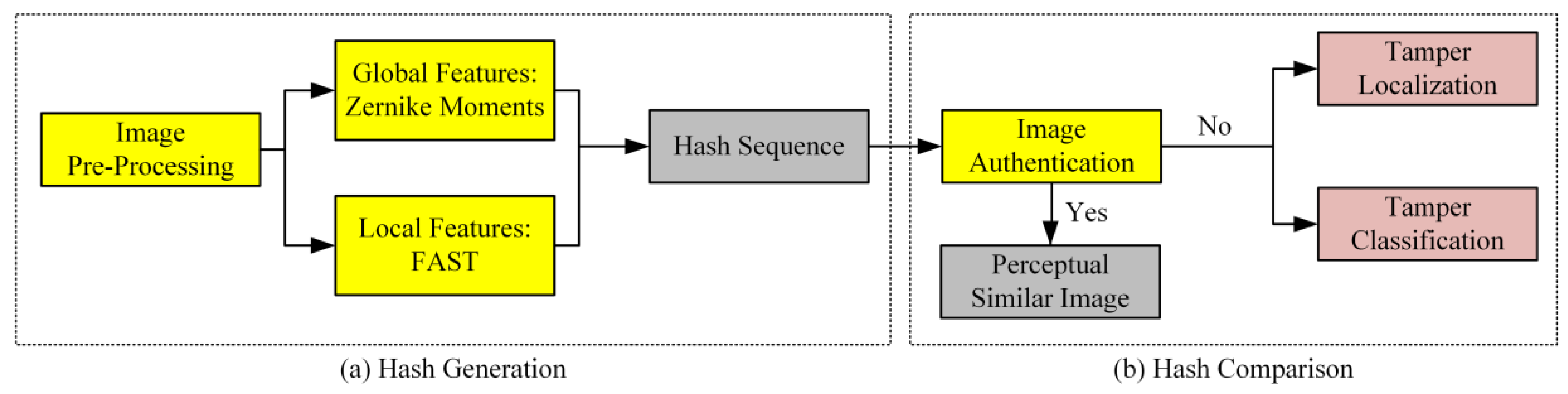
3. Perceptual Hashing Algorithm Combining Zernike Moments and FAST

A HRRS image perception hashing algorithm combining Zernike moments and FAST is proposed, as shown in Figure 4. Zernike moments are used to describe global features, and the FAST algorithm is used to obtain local features. The global features and local features are combined to generate a hash sequence.

3.1. HRRS Images Pre-Processing

For ordinary remote sensing images, image fusion algorithms are used for pre-processing. For multi-band remote sensing images, data can be extracted separately for independent authentication. The image perceptual hash algorithm usually normalizes the original image to a uniform size for authentication. Considering that the HRRS image has the characteristics of large image size and rich details, we pre-process the original image $D$ by means of grid division and divide the original image into sub-blocks of size $m\times m$. In HRRS images, it is recommended to use a 256 × 256 grid unit size for grid division, and sensitivity analysis of this size will be given later. For the area with less than m pixels at the boundary, 0 value is used to complete.

The original data $D$ can be divided into a grid unit area of $W\times H$, and the divided grid units is denoted as $D_{wh}\left(w=1,2,\dots ,W;h=1,2,\dots ,H\right)$, where w and h represent the locations of the grid units. Figure 5 shows the result of 256 × 256 grid division on a HRRS image with a size of 5031 × 4516. The following hash generation and hash discrimination processes will be performed at the grid unit level.

3.2. HRRS Image Hash Generation

3.2.1. Global Features Extraction

As mentioned above, the global features of the grid unit are obtained by calculating the Zernike moment of the grid unit data. Since the low-order Zernike moments can well represent the texture information of the image, the order of the Zernike moment does not need to be too high. In this paper, the order $n$ of moment is chosen $n=$ 5, which is sufficient to represent the texture information of the image [44].

As shown in

Table 1. The number of zernike moments of each order.

Order	Zernike Moments	Number of the Moments
0	Z0,0	1
1	Z1,1,	1
2	Z2,0, Z2,2	2
3	Z3,1, Z3,3	2
4	Z4,0, Z4,2, Z4,4	3
5	Z5,1, Z5,3, Z5,5	3

, all elements of the five-order Zernike moments are obtained, and finally, 12 Zernike moments can be obtained. The magnitude of a Zernike moment is recorded as the eigenvalue a, so for a grid unit $D_{wh}$, the vector a in 5-order Zernike moments is a 12-dimensional feature space, which is recorded as $Z_{wh}=\left(a_1,a_2,\dots ,a_{12}\right)$.

3.2.2. Local Features Extraction

The FAST algorithm is used to extract the local features of the grid units. The FAST algorithm can extract a series of key points $F$ of the grid unit, i.e., $F=\left\{F_1,F_2,\dots ,F_n\right\}$. In order to make the extracted feature more robust and reduce the length of hash sequence, the key points extracted by FAST will be further screened as follows:

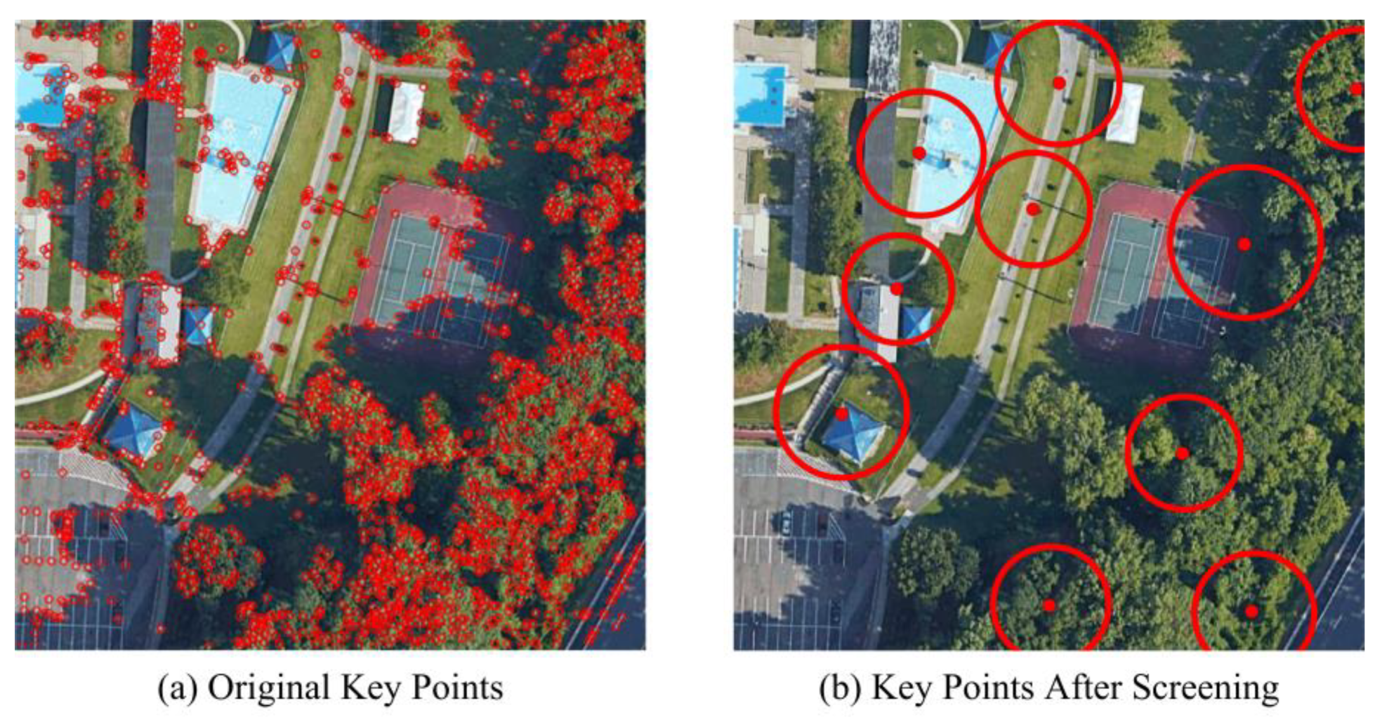
• Sort all the feature points from large to small according to the response $R$, and define the sorted feature point set as $F_{new}$. A new key point set is defined as $S$, and an auxiliary circle set $C^{\prime }$ is defined.
• The screening algorithm is executed from $F_1$. Let the current point be $F_x(0<x<n)$, draw a circle $C_x$ with the coordinates of $F_x$ as the center, and the response $R$ as the radius. If $C_x$ does not intersect any circle in $C^{\prime }$, then $F_x$ is added to $S$, and $C_x$ is added to $C^{\prime }$.
• Step 2 is performed in sequence until there are 10 points in $S$, and the screening is completed.
• For each point in $F_{new}$, the average luminance feature is added to the key point description. The average luminance A is defined as the mean value of the pixel in the square with response $R$ as the side length and the key point coordinate $\left(x,y\right)$ as the center.

According to the principle of FAST, the larger the response, the greater the difference between key point and surrounding points. If content retention operations (such as Gaussian Filter) are applied to the image, the features of large response are not easy to be erased, yet. So, FAST key points with larger response are more stable than those with low response, and the key points set obtained through screening will be more robust. Screening using the intersection of circles can make the key points as evenly distributed as possible throughout the grid unit, and shorten the length of the hash sequence as much as possible. Since key points are extracted at the grid unit level, which is in a small region, the number of selected points need not be too large. In this paper, the number of key points in each grid unit is chosen to be $n=10$, taking into account the length of hash sequence and calculation efficiency. Therefore, the final set of key points is $S_{wh}=\left\{S_1,S_2,\dots ,S_{10}\right\}$. Figure 6 shows the key points of a grid unit after screening.

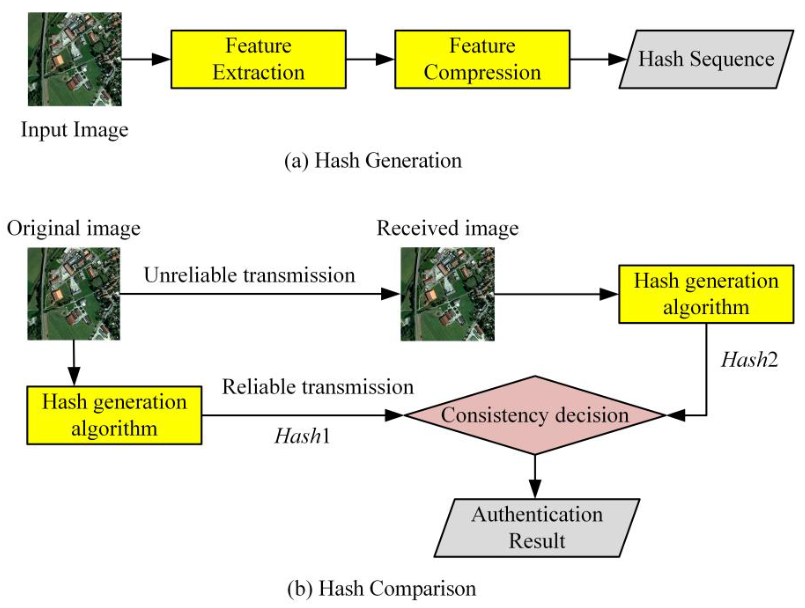
3.2.3. Hash Construction

The hash value $H_{wh}$ of a grid unit $D_{wh}$ is composed of $Z_{wh}$ and $S_{wh}$, i.e., $H_{wh}=\left\{Z_{wh},S_{wh}\right\}$, which is called a unit hash. For each element in a unit hash, the integer truncation method is used to process the data in order to further shorten the hash length. The final unit hash length is (12 + (4 × 10)) × 8 Bit = 416 Bit. For a HRRS image, the hash sequence is the set of hashes of each unit, i.e., $H\left(D\right)=\left\{H{\left(D\right)}_{11},\dots ,H{\left(D\right)}_{wh}\right\}\left(w=1,2,\dots ,W;h=1,2,\dots ,H\right)$. The length of the final perception hash sequence of the image depends on the size of the image. Meanwhile, in order to ensure the security of authentication, the method of Logistic transformation [45] is used to conduct pseudo-random scrambling of the original hash $H\left(D\right)$, and the scrambling key is set as K.

3.3. Hash Comparison

As mentioned above, in a typical data sharing case, the transmission of data generally runs in an unreliable channel, and the hash sequence $H\left(D\right)$ generated from the original data together with the key K need to be transmitted to the receiver through the reliable channel. The receiver uses the same hash generation algorithm as the original data to generate the hash sequence $H\left(D^{\prime }\right)$ of the data to be authenticated, and decrypts the original hash sequence $H\left(D\right)$ with the key K.

3.3.1. Global Features Discrimination

Since the Zernike moment has sufficient ability to describe the texture information of the image [39], the integrity authentication can be implemented by the Zernike moments. Meanwhile, based on the good detail feature recognition ability of FAST, it is applied to tampering localization. Calculate the similarity $Sim\left(w,h\right)$ of the Zernike moments characteristics of the grid unit in the same position of $H\left(D\right)$ and $H\left(D^{\prime }\right)$ one by one. The similarity measurement method is to calculate their Euclidean distance, as shown in Formula (7):

$$Sim\left(w,h\right)=\parallel Z{\left(D\right)}_{wh}-Z{\left(D^{\prime }\right)}_{wh}\parallel {}_2.$$

(7)

By combining the judgment thresholds $T_1$ and $T_2(0<T_1<T_2)$, the authentication results will be divided into three categories:

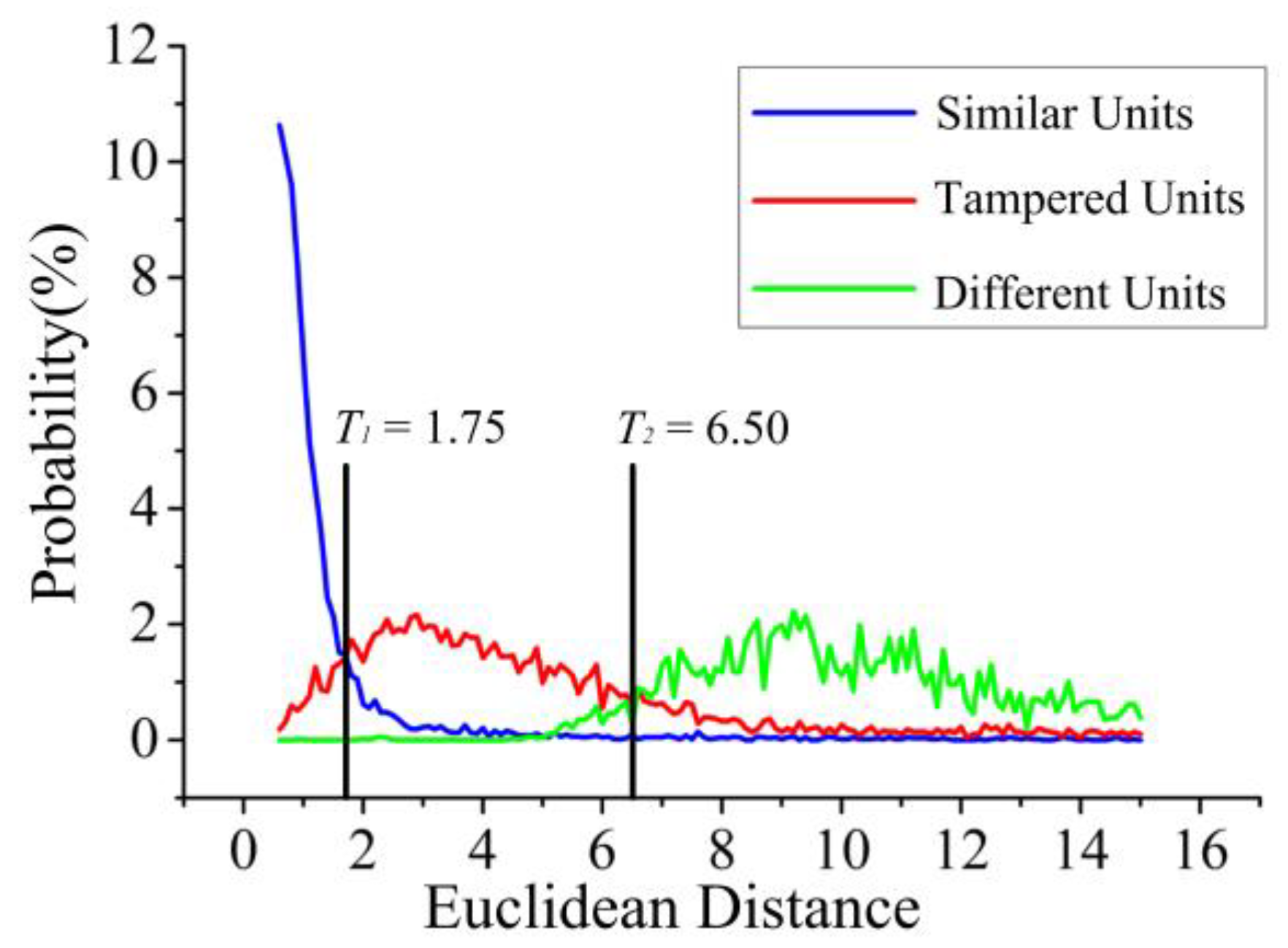
• $0\le Sim\left(w,h\right)<T_1$: Group 1, consistent with original data perception and passed authentication;
• $T_1\le Sim\left(w,h\right)<T_2$: Group 2, the grid unit has been tampered and does not pass the authentication, which needs to be tamper-localized;
• $Sim\left(w,h\right)\ge T_2$: Group 3, there are totally different content data in the grid unit, which cannot pass the authentication. The whole grid unit is marked as tampered.

The determination of the thresholds $T_1$ and $T_2$ will be discussed in the experimental section.

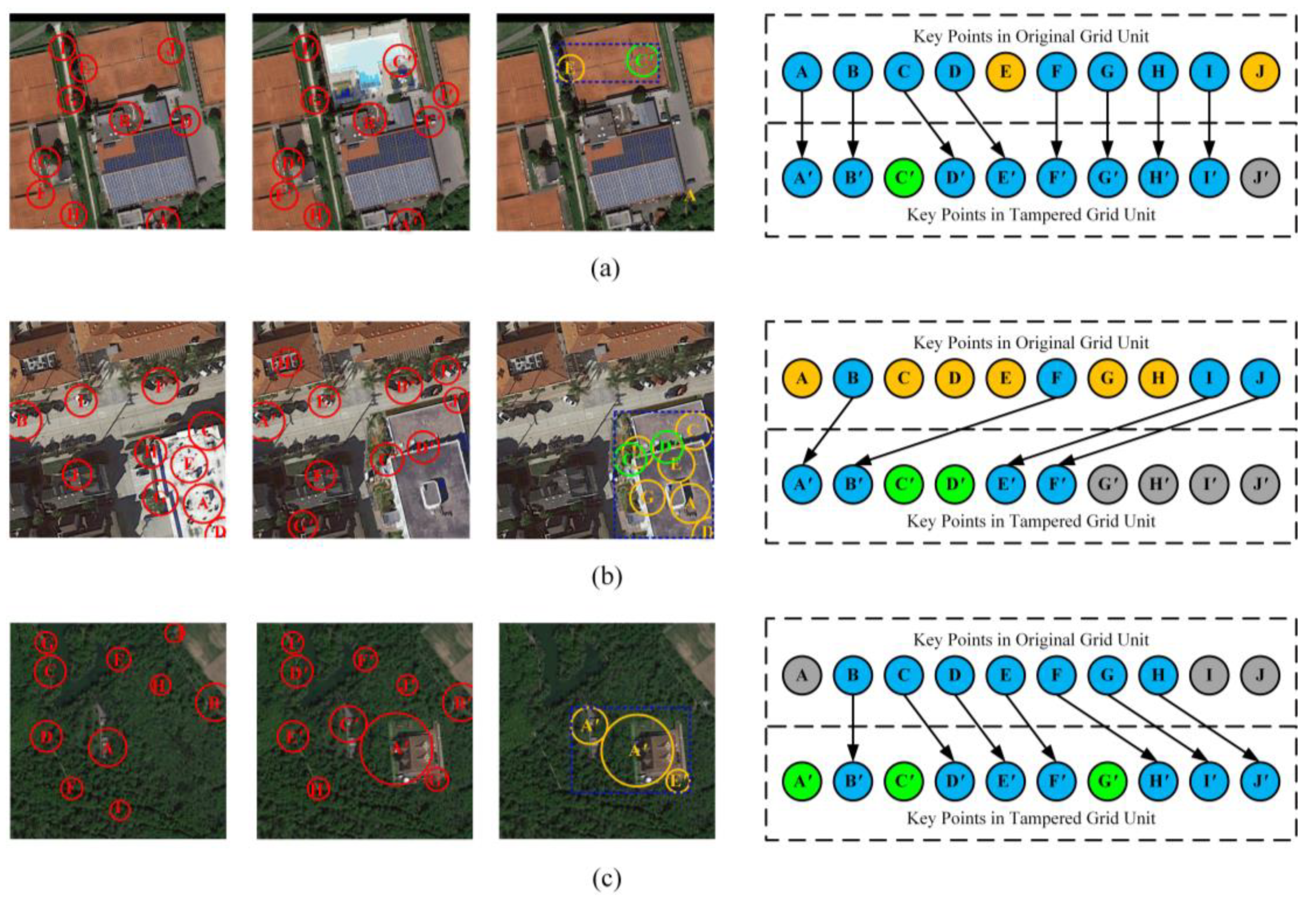
3.3.2. Local Features Discrimination

From an authentication perspective, if a grid unit fails to pass authentication, it indicates that the whole HRRS image has not lost its “integrity”. However, with respect of the need of tamper localization, it is necessary to determine the similarity of all grid units to reach a more explanatory conclusion. For the grid units in Group 2, as mentioned above, the FAST key points need to be further processed.

The processing method is illustrated with examples, as shown in Figure 7. The hash sequences of Figure 7 are presented in Appendix A. The processing method is as follows:

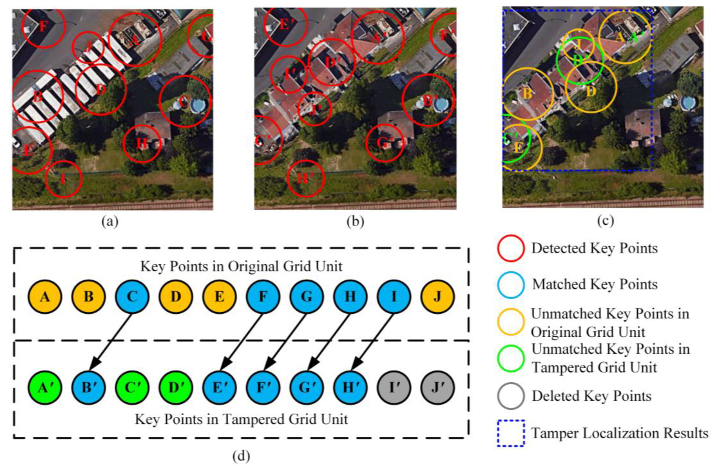
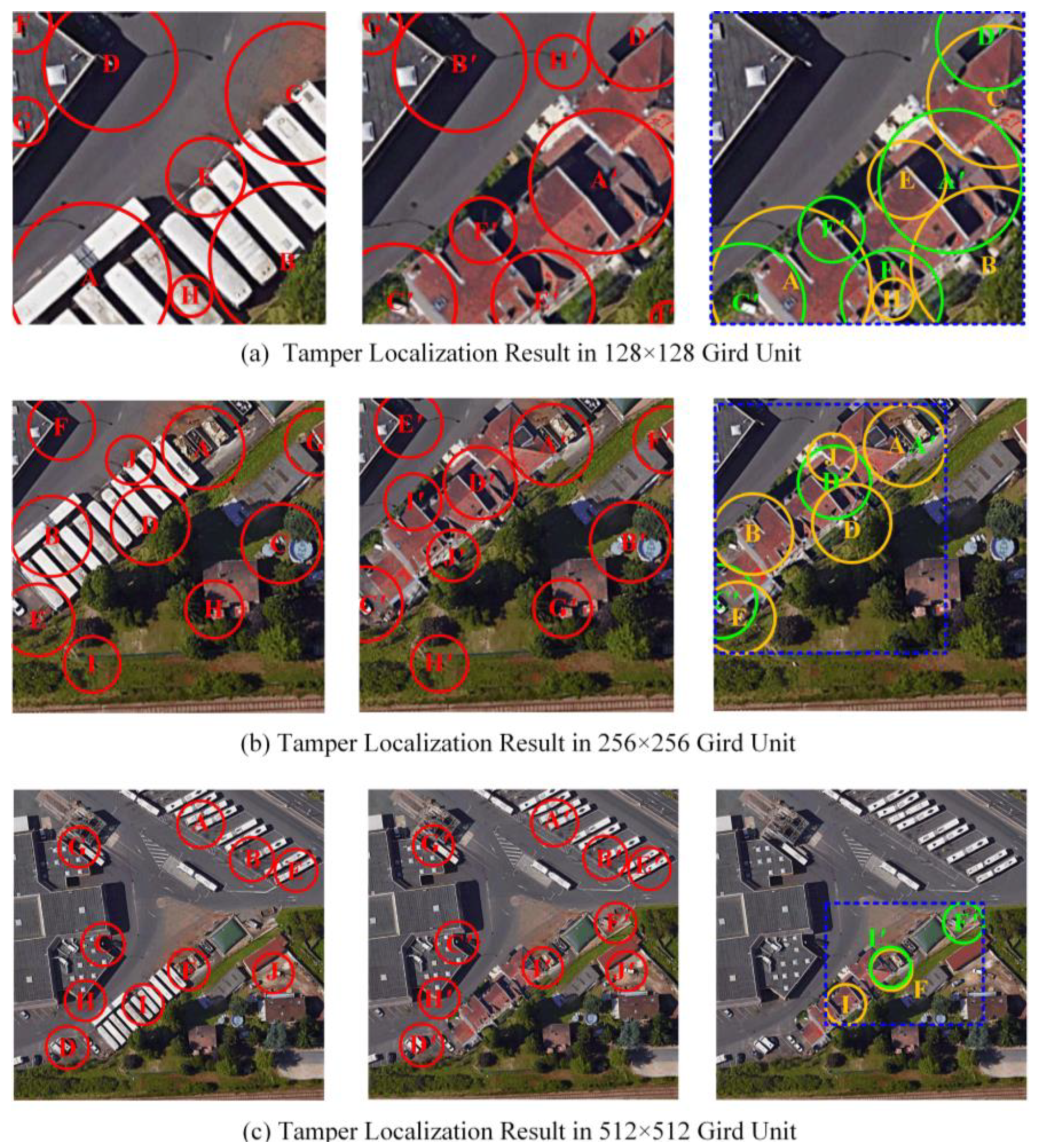
• Using the Fast Library for Approximate Nearest Neighbors (FLANN) method for the key points set $S{\left(D\right)}_{wh}$ of the original grid unit and the feature point set $S{\left(D^{\prime }\right)}_{wh}$ for the unit to be authenticated to making a match. FLANN is an efficient key point matching method, which needs to consider the matching threshold. We set the matching threshold to 0.8, which is the threshold recommended by Muja [46] in his paper. As shown in Figure 7d, the blue points are the five pairs of key points that were successfully matched.
• Delete the points whose average luminance has not changed significantly. For the unmatched key points in original grid units, if their average luminance does not change significantly compared with the tampered grid unit, they should be deleted. Otherwise, the key points should be retained. Since the average luminance of the key points in the original grid unit is known, the average luminance of the tampered grid unit can be calculated at the same position, so the average luminance change of these key points can be obtained. Which means, when:

  $$\left|A\left(x,y\right)-A^{\prime }\left(x,y\right)\right|<T_L.$$

  (8)
• Delete the point. To enhance robustness, the average brightness threshold is set to $T_L=2$. As shown in Figure 7c, the points “A”, “B”, “D”, “E”, and “J” are all retained because the average brightness around them has changed. Delete unmatched key points at the end of each sets. After matching, if there is still an unmatched key point at the end of $S{\left(D^{\prime }\right)}_{wh}$ and $S{\left(D\right)}_{wh}$, remove it. However, if any of these points are determined to have changed in average luminance in the previous step, they will not be deleted. Since the number of a key points set is fixed at 10, a point at the end that is not matched does not mean that it has been tampered with, but that its corresponding matching point may be ranked after the 10th place of another set. For instance, “I′” and “J′” are deleted in this example. We can find that although they are not matched, their regions have not been tampered with.
• For the circle formed by all remaining feature points, the minimum external rectangle is constructed, which is the tamper region. As shown in Figure 7c, the remaining key points are “A”, “B”, “D”, “E”, “J”, “A′”, “C′”, and “D′”, and the blue rectangle is the tamper localization result.
• Three special cases are considered: If all the key points are not matched successfully it means that the grid unit is mistakenly divided into “Group 2”. Thus, this grid unit should be re-divided into “Group 3”, since all the key points have been tampered with. If all the key points are matched successfully, it means that the micro-tamper was not detected. In extreme cases, if the number of key points after screening is less than 10, the above method can still be used for key points matching and tamper localization—certainly with a lower accuracy.

4. Experiment and Analysis

In order to verify the validity and universality of the algorithm, this paper selects 100 images from the DOTA [47] HRRS image database to construct a dataset, the size of which ranges from 7568 × 5619 to 1444 × 1727. DOTA dataset is composed of three data sources: Google Earth, GF-2 and JL-1. These data are all sub-meter resolution remote sensing images, among which the resolution of Google Earth image is 0.5 m, the resolution of GF-2 image is 0.8 m, and the resolution of JL-1 image is 0.72 m.

4.1. Grid Unit Size Sensitivity Analysis

The size of the grid division $m$ can be considered as the protection level the user wishes to assign to the algorithm. The size of grid units may directly affect the granularity of authentication. If $m$ is too large, many details of the HRRS image will be lost, while if $m$ is too small, the computational complexity will be greatly increased.

Table 2. Calculation time and Euclidean distance of different grid sizes.

Grid Size (pixel)	Calculation Time (s)	Euclidean Distance of Different Grid Units	Euclidean Distance of Similar Grid Units
512	3.51	3.35	0.02
256	5.03	8.62	0.02
128	10.07	8.73	0.01

shows the computing time of Zernike moment under different grid sizes and the Euclidean distance between similar grid units and different grid units. The data in the table are the mean values of the data tested on 20 HRRS images. The calculation time is the sum of grid division time and Zernike moment calculation time. The calculation time was tested on PC platforms with Anaconda3(Python3.7), Dual i5-3230m CPU and 12G RAM.

As can be seen from the table, although the 512 × 512 grid division has the shortest calculation time, it has poor discrimination to the data. Selecting a 256 × 256 grid unit for authentication can obtain the optimal solution between algorithm complexity and content recognition capability.

In addition, an experiment on comparing the tamper localization ability under different grid sizes is given in Figure 8. Three tampered images with different grid sizes are selected for multi-scale tampering localization tests, which reflect the same tampered area. The results show that the algorithm we proposed can recognize the tamper location effectively at different grid sizes. It should be noted that the tamper area in Figure 8a covers most areas in the grid unit, so the tamper location is relatively large. In Figure 8c, it is possible that minor tampering with the data cannot be identified due to the expanded grid scope (although this tampering area is identified in our example). Therefore, from this aspect, it is also recommended to use 256 × 256 size for grid division.

4.2. Global Features Threshold Analysis

In order to give a reasonable threshold for the global feature extraction, a large amount of data needs to be tested.

The 100 images in the “original dataset” were processed without changing the content to produce a “similar data set” consisting of 700 images. These operations that do not change content include LSB watermark embedding, format conversion to BMP, format conversion to PNG, Gaussian filtering (${\sigma }^2=0.1,{\sigma }^2=1$), and JPEG compression ($Q=99\%,Q=90\%$). After the grid division, there are 6337 grid units in the original dataset, and 44,359 grid units in the similar dataset. Therefore, 44,359 pairs of grid unit with similar contents can be generated.

Tamper attack is applied to the grid units in the original dataset to obtain a “tampered dataset” consisting of 6337 grid units. The method of tampering is to randomly replace regions ranging from 15% to 25% of the original grid unit, which can generate 6337 pairs of grid units whose contents have been tampered with. To achieve this, we built 40 tamper templates, ranging in size from 100 × 100 to 128 × 128. Among these templates, there are 10 in size 100 × 100, 10 in size 110 × 110, 10 in size 120 × 120, and 10 in size 128 × 128. These templates are randomly assigned to each of the original grid cells to replace portions of the original data.

By completely replacing the grid units in the original database, a “different dataset” can be obtained, and 6337 pairs of grid unit pairs with different contents can be generated.

The Euclidean distance between 44,359 similar unit pairs, 6337 tampered unit pairs and 6337 different unit pairs is calculated to obtain the Euclidean distance probability distribution diagram, as shown in Figure 9. As can be seen from the figure, when the threshold $T_1=1.75$ and the threshold $T_2=6.50$, the best discrimination of different datasets can be obtained. Additionally, all the thresholds used in this algorithm are presented in Appendix B.

4.3. Robustness Tests

A good perceptual hashing algorithm should be robust to content retention operations. As described in Section 4.2, the 44,359 grid units in the “similar dataset” are all data that have undergone content retention operations. They should theoretically pass the integrity authentication. The accuracy of the algorithm can be obtained through integrity authentication test of the “similar dataset”, as shown in

Table 3. Robustness testing results.

Content Retention Operation.	Accuracy (%)
LSB Watermark Embedding	99.99
Format Conversion to BMP	100.00
Format Conversion to PNG	100.00
JPEG Compression ($Q=99\%$)	99.96
JPEG Compression ($Q=90\%$)	99.93
Gaussian Filtering (${\sigma }^2=0.1$)	100.00
Gaussian Filtering (${\sigma }^2=1$)	83.81

.

According to the data in the table, the proposed algorithm is nearly 100% robust to LSB watermark embedding, format transformation, JPEG compression and Gaussian filtering (${\sigma }^2=0.1$), while showing a relatively weak result to Gaussian filtering (${\sigma }^2=1$). The reason is that the Gaussian filter is a holistic filter. When ${\sigma }^2=1$, the information of the image may change greatly. Overall, the algorithm is still robust to a variety of content retention operations.4.4. Tamper Detection Tests.

While maintaining the sensitivity to “content retention operations”, the sensitivity to “content tampering operations” also needs to be considered. A good integrity authentication algorithm needs to have a good distinction between content retention operations and content tampering operations. Furthermore, a distinction between “Tampered Dataset” and “Different Dataset” is also required. In order to verify the comprehensive performance of the algorithm, the confusion matrix in three datasets (Similar Dataset, Tampered Dataset and Different Dataset) is given in

Table 4. Confusion matrix for similar dataset, tampered dataset and different dataset.

Predicted Value.	Real Value
	Similar Unit	Tampered Unit	Different Unit
Similar Unit	43,463	356	49
Tampered Unit	732	4382	1149
Different Unit	164	1599	5139

.

True Positive Rate ($TPR$) and False Positive Rate ($FPR$) is commonly used to determine the comprehensive performance of algorithms. The definition of TPR and FPR is given in Formula (9):

$$TPR=\frac{TP}{TP+FN},FPR=\frac{FP}{FP+TN}.$$

(9)

In this formula, $TP$ refers to the True Positive, $FP$ refers to the False Positive, $FN$ refers to the refers to the False Negative, and $TN$ refers to the True Negative. TPR represents the proportion of positive instances recognized by the algorithm to all positive instances, and TFR represents the proportion of negative instances misclassified by algorithm to all negative instances.

Table 5. TPR and FPR Value of Similar Dataset, Tampered Dataset and Different Dataset.

Evaluation Index	Dataset
	Similar Dataset	Tampered Dataset	Different Dataset
TPR	97.98% (TPRS)	69.15% (TPRT)	81.09% (TPRD)
FPR	3.19% (FPRS)	3.37% (FPRT)	3.47% (FPRD)

shows the TPR and FPR value of each dataset.

$TP{R}_S$ represents the robustness of the algorithm, that is, the probability that the data can pass the integrity authentication after content retention operations. $FP{R}_S$ represents the probability that the data is incorrectly marked as “pass the integrity authentication” after content tampering operations. In this experiment, $TP{R}_S=97.98\%$, and $FP{R}_S=3.19\%$. It can be seen that the algorithm is highly robust to content retention operations and highly sensitive to content tampering options. In another word, the algorithm has a strong distinguishing ability between content retention operation and content tampering operation.

However, the values of TPR_T and TPR_D are not very ideal. As can be seen from Table 4, some Tamper Units are considered Different Units, and some Different Units are considered Tamper Units. The reason is that the size of tampered area cannot affect the intensity of tampering linearly. For example, embedding a black tamper area in a white image has a great impact on the Zernike moments, while replacing one lawn with another lawn has a relatively small impact on the Zernike moments. In principle, the distinguishing ability between Tamper Units and Different Units only affects the result of tamper localization. Since the tamper localization is implemented in grid unit scale, the results will not be greatly affected.

4.4. Tamper Localization Tests

In order to verify the effectiveness of the algorithm for tamper localization, we performed tamper localization experiments on the grid unit scale and the whole image scale, respectively.

4.4.1. Tamper Localization Tests in Grid Units

In this experiment, the tamper localization results of three tampered grid units are shown. The key points matching method described above is implemented to localize the tampered area. As shown in Figure 10, the tampered areas in these grid units were found and identified. This shows that the tampering localization method we designed can provide a relatively accurate tampering positioning results while maintaining the abstraction of hash sequence. In essence, if a large number of key points are selected, the tampered area can be depicted more accurately. However, due to the requirements of hash abstraction, a relatively reasonable result can still be obtained by using only 10 key points.

4.4.2. Tamper Localization Tests in Whole Images

Because it is difficult to construct a convincing tampered image, we selected six HRRS images for tamper localization test in the whole image scale. As shown in

Table 6. Tamper detection testing results.

Image Size.	Division Granularity	Original Data	Tampered Data	Tamper Localization
4020 × 2444	16 × 10
3004 × 2987	12 × 12
1703 × 1880	7 × 8
1954 × 1818	8 × 8
1945 × 1948	8 × 8
2098 × 1642	9 × 7

, tamper localization results of six tamper images are obtained. A total of 71 grid units were affected by “tamper attack”, of which 68 tampered units were detected by this algorithm, with a tamper recognition rate of 95.77%. Three tampered grid units were not identified because it involved a very small area. As has been explained in Section 4.3, the distinguishing ability between Tamper Units and Different Units is relatively low, and some grid units are wrongly classified. Theoretically, because the results of tamper localization have spatial relevance, that is, some tampered areas are interconnected. Thus, a convex hull can be built to further simulate the tamper position. However, considering the randomness of tampering, it is difficult to determine whether these tampering concepts have spatial correlation, so this method was not adopted. However, at the whole image scale, the accuracy of tamper localization is still accurate, and most of tampered areas can be identified and located.

4.5. Algorithm Security Analysis

The security of the perceptual hash algorithm mainly refers to the unidirectivity of the hash sequence, that is, image information cannot be deduced by the hash sequence. Since we used Logistic transform to encrypt the hash sequence, the unidirectivity of the hash sequence can be ensured. In essence, the information of the image is transformed into a meaningless string, which guarantees the security of the algorithm. Of course, in the specific implementation process, DES and AES and other encryption algorithms can also be considered as the hash sequence encryption method. However, this is not the focus of this article and will not be described in detail here.

4.6. Comparison with Existing Algorithms

We compare this algorithm with the existing perceptual hash algorithm, which includes both digital image perceptual hash algorithms [31,33,34,35,36,37] and HRRS image perceptual hashing algorithm [28,29].

Table 7. Comparison between different algorithms.

Algorithm	DCT Based [33,34]	DWT Based [35,36]	Zernike Moments Based [37]	SIFT Based [31]	Canny Based [28]	U-Net Based [29]	Proposed Method
Feature Used	Global	Global	Global	Local	Local	Local	Global and Local
Time Cost of Feature Extraction	0.016	0.484	0.336	2.281	0.482	/	0.347
Robust Against Content Retention Options	Yes	Yes	Yes	Yes	Yes	Yes	Yes
Tamper Identification	Yes	Yes	Yes	Yes	Yes	Yes	Yes
Tamper Localization	No	No	No	Yes	Yes	Yes	Yes
Tamper Localization Granularity	/	/	/	Rectangle	Grid	Grid	Sub-Grid

shows the comparison results of these algorithms.

Due to the use of the FAST algorithm for feature extraction, the execution speed of the algorithm is greatly improved compared with that based on SIFT key point detection algorithm. Meanwhile, due to the combination of global and local features, the algorithm can refine the positioning results to the level of the sub-grid. In other words, the grid is only the basis of tamper location, and the final tamper location accuracy will be higher than the grid size.

5. Conclusions

In this paper, by combining the ability of the Zernike moment to distinguish image content and the FAST algorithm to identify key points, a HRRS image perceptual hashing algorithm was proposed. The algorithm has strong robustness to the content retention operation, has effective recognition ability for content tampering operations, and can achieve tampering localization. The contributions of this paper are as follows:

• By applying the idea of multi-feature combination to the authentication of HRRS images has enhanced reliability compared to existing HRRS image authentication algorithms.
• Compared with the existing digital image perceptual hashing algorithms, the introduction of the FAST algorithm greatly improves the extraction efficiency of key points. This would be more practical for HRRS images with a large image size.
• A series of databases were constructed to analyze the judgment threshold. Compared with the existing algorithms, the judgment is based on experimental threshold, which improves the interpretability and accuracy.

In future research, a further detailed understanding and use of FAST descriptors will be considered in order to obtain higher tamper localization accuracy. Because the method of grid division is used to improve the accuracy of authentication, the total length of hash sequence depends on the size of image, which inevitably leads to the excessively long image hash sequence. It is also an important issue to explore the way to further compress hash sequences in future research. Ideally, the number of key points can be changed adaptively according to the content of the image, but this may require the use of machine learning methods, which will also involve a lot of problems about image semantic analysis. We hope to have a further research on it in the future.

References

1. Meng-Dawn, C.; Edwin, C. A study of extractive and remote-sensing sampling and measurement of emissions from military aircraft engines. Atmos. Environ. 2010, 44, 4867–4878. [Google Scholar]
2. Sawaya, K.E.; Olmanson, L.G.; Heinert, N.J.; Brezonik, P.L.; Bauer, M.E. Extending satellite remote sensing to local scales: Land and water resource monitoring using high-resolution imagery. Remote Sens. Environ. 2003, 88, 144–156. [Google Scholar] [CrossRef]
3. Yamazaki, F.; Matsuoka, M. Remote sensing technologies in post-disaster damage assessment. J. Earthq. Tsunami 2007, 1, 193–210. [Google Scholar] [CrossRef] [Green Version]
4. Bio, A.; Gonçalves, J.A.; Magalhães, A.; Pinheiro, J.; Bastos, L. Combining Low-Cost Sonar and High-Precision Global Navigation Satellite System for Shallow Water Bathymetry. Estuaries Coasts 2020, 1–12. [Google Scholar] [CrossRef]
5. Ding, K. Perceptual Hashing Based Authentication Algorithm Research for Remote Sensing Image. Ph.D. Thesis, Nanjing Normal University, Nanjing, China, 2013. [Google Scholar]
6. Hambouz, A.; Shaheen, Y.; Manna, A.; Al-Fayoumi, M.; Tedmori, S. Achieving Data Integrity and Confidentiality Using Image Steganography and Hashing Techniques. In Proceedings of the 2nd International Conference on new Trends in Computing Sciences (ICTCS), Amman, Jordan, 9–11 October 2019; IEEE: New York, NY, USA, 2019; pp. 1–6. [Google Scholar]
7. Iqbal, S. Digital Signature Based on Matrix Power Function. Ph.D. Thesis, Capital University, Columbus, OH, USA, 2019. [Google Scholar]
8. Mohanarathinam, A.; Kamalraj, S.; Venkatesan, G.P.; Ravi, R.V.; Manikandababu, C.S. Digital watermarking techniques for image security: A review. J. Ambient Intell. Humaniz. Comput. 2019, 1–9. [Google Scholar] [CrossRef]
9. Du, L.; Ho, A.T.; Cong, R. Perceptual hashing for image authentication: A survey. Signal Process. Image Commun. 2020, 81, 115713. [Google Scholar] [CrossRef]
10. Long, S. A Comparative Analysis of the Application of Hashing Encryption Algorithms for MD5, SHA-1, and SHA-512. J. Phys. Conf. Ser. 2019, 1314. [Google Scholar] [CrossRef]
11. Li, L.; Zhang, C.; Li, D. Remote sensing image anti-modification in land consolidation based on XOR LSB algorithm. Trans. Case 2008, 24, 97–101. [Google Scholar]
12. Serra-Ruiz, J.; Megías, D. A novel semi-fragile forensic watermarking scheme for remote sensing images. Int. J. Remote Sens. 2011, 32, 5583–5606. [Google Scholar] [CrossRef] [Green Version]
13. Zhang, X. Research on Integrity Authentication Algorithm of Remote Sensing Image Based on Fragile Watermarking. Master’s Thesis, Nanjing Normal University, Nanjing, China, 2014. [Google Scholar]
14. Qin, Q.; Wang, W.; Chen, S.; Chen, D.; Fu, W. Research of digital semi-fragile watermarking of remote sensing image based on wavelet analysis. In Proceedings of the 2004 IEEE International Geoscience and Remote Sensing Symposium (IGARSS), Anchorage, AK, USA, 20–24 September 2004; IEEE: New York, NY, USA, 2004; Volume 4, pp. 2542–2545. [Google Scholar]
15. Serra-Ruiz, J.; Megías, D. DWT and TSVQ-based semi-fragile watermarking scheme for tampering detection in remote sensing images. In Proceedings of the 2010 Fourth Pacific-Rim Symposium on Image and Video Technology, Washington, DC, USA, 14–17 November 2010; IEEE: New York, NY, USA, 2010; pp. 331–336. [Google Scholar]
16. Tong, D.; Ren, N.; Zhu, C. Secure and robust watermarking algorithm for remote sensing images based on compressive sensing. Multimed. Tools Appl. 2019, 78, 16053–16076. [Google Scholar] [CrossRef]
17. Niu, X.M.; Jiao, Y.H. An overview of perceptual hashing. Acta Electron. Sin. 2008, 36, 1405–1411. [Google Scholar]
18. Sarohi, H.K.; Khan, F.U. Image retrieval using perceptual hashing. IOSR-JCE 2013, 9. [Google Scholar] [CrossRef]
19. Nagarajan, S.K.; Saravanan, S. Content-based medical image annotation and retrieval using perceptual hashing algorithm. IOSR J. Eng. 2012, 2, 814–818. [Google Scholar] [CrossRef]
20. He, S.; Zhao, H. A retrieval algorithm of encrypted speech based on syllable-level perceptual hashing. Comput. Sci. Inf. Syst. 2017, 14, 703–718. [Google Scholar] [CrossRef]
21. Zhang, Q.Y.; Xing, P.F.; Huang, Y.B.; Dong, R.H.; Yang, Z.P. An efficient speech perceptual hashing authentication algorithm based on wavelet packet decomposition. J. Inf. Hiding Multimed. Signal Proc. 2015, 6, 311–322. [Google Scholar]
22. Wang, H.; Yin, B. Perceptual hashing-based robust image authentication scheme for wireless multimedia sensor networks. Int. J. Distrib. Sens. Netw. 2013, 9, 791814. [Google Scholar] [CrossRef]
23. Renza, D.; Vargas, J.; Ballesteros, D.M. Robust Speech Hashing for Digital Audio Forensics. Appl. Sci. 2020, 10, 249. [Google Scholar] [CrossRef] [Green Version]
24. Srivastava, M.; Siddiqui, J.; Ali, M.A. A Review of Hashing based Image Copy Detection Techniques. Cybernet. Inf. Tech. 2019, 19, 3–27. [Google Scholar] [CrossRef] [Green Version]
25. Liu, S.; Huang, Z. Efficient Image Hashing with Geometric Invariant Vector Distance for Copy Detection. ACM Trans. Multim. Comput. 2019, 15, 1–22. [Google Scholar] [CrossRef]
26. Liu, C.; Ma, J.; Tang, X.; Zhang, X.; Jiao, L. Adversarial Hash-Code Learning for Remote Sensing Image Retrieval. In Proceedings of the 2019 IEEE International Geoscience and Remote Sensing Symposium (IGARSS), Yokohama, Japan, 28 July–2 August 2019; IEEE: New York, NY, USA, 2019; pp. 4324–4327. [Google Scholar]
27. Ding, K.; Zhu, Y.; Zhu, C. A Perceptual Hash Algorithm Based on Gabor Filter Bank and DWT for Remote Sensing Image Authenticaton. J. Chi. Rail Soci. 2016, 7, 70–76. [Google Scholar]
28. Ding, K.; Meng, F.; Liu, Y.; Xu, N.; Chen, W. Perceptual Hashing Based Forensics Scheme for the Integrity Authentication of High-Resolution Remote Sensing Image. Information 2019, 9, 229. [Google Scholar] [CrossRef] [Green Version]
29. Ding, K.; Yang, Z.; Wang, Y.; Liu, Y. An improved perceptual hash algorithm based on u-net for the authentication of high-resolution remote sensing image. Appl. Sci. 2019, 9, 2972. [Google Scholar] [CrossRef] [Green Version]
30. Haitsma, J.; Kalker, T.; Oostveen, J. Robust audio hashing for content identification. In International Workshop on Content-Based Multimedia Indexing; University of Brescia: Brescia, Italy, 2001; Volume 4, pp. 117–124. [Google Scholar]
31. Ouyang, J.; Liu, Y.; Shu, H. Robust hashing for image authentication using SIFT feature and quaternion Zernike moments. Multimed. Tools Appl. 2017, 76, 2609–2626. [Google Scholar] [CrossRef]
32. Yang, G.; Chen, N.; Jiang, Q. A robust hashing algorithm based on SURF for video copy detection. Comput. Secur. 2012, 31, 33–39. [Google Scholar] [CrossRef]
33. Sengar, S.S.; Mukhopadhyay, S. Moving object tracking using Laplacian-DCT based perceptual hash. In Proceedings of the 2016 International Conference on Wireless Communications, Signal Processing and Networking (WiSPNET), Chennai, India, 23–25 March 2016; IEEE: New York, NY, USA, 2019; pp. 2345–2349. [Google Scholar]
34. Li, Y.J.; Li, J.B. DCT and perceptual hashing based to identify texture anti-counterfeiting tag. Appl. Res. Comput. 2014, 31, 3734–3737. [Google Scholar]
35. Hu, M.K. Visual pattern recognition by moment invariants. IEEE Trans. Inf. Theory 1962, 8, 179–187. [Google Scholar]
36. Govindaraj, P.; Sandeep, R. Ring partition and dwt based perceptual image hashing with application to indexing and retrieval of near-identical images. In Proceedings of the 2015 Fifth International Conference on Advances in Computing and Communications (ICACC), Manipal, Karnataka, India, 2–4 September 2015; IEEE: New York, NY, USA, 2019; pp. 421–425. [Google Scholar]
37. Zhao, Y.; Wang, S.; Feng, G.; Tang, Z. A robust image hashing method based on Zernike moments. J. Comput. Inf. Syst. 2010, 6, 717–725. [Google Scholar]
38. Khotanzad, A.; Hong, Y.H. Invariant image recognition by Zernike moments. IEEE Trans Pattern Anal. 1990, 12, 489–497. [Google Scholar] [CrossRef] [Green Version]
39. Harris, C.G.; Stephens, M. A combined corner and edge detector. In Proceedings of the 4th Alvey Vision Conference; Alvey: Manchester, UK, 1988; Volume 15, pp. 10–5244. [Google Scholar]
40. Lowe, D.G. Distinctive image features from scale-invariant keypoints. Int. J. Comput. Vis. 2004, 60, 91–110. [Google Scholar] [CrossRef]
41. Bay, H.; Ess, A.; Tuytelaars, T.; Van Gool, L. Speeded-up robust features (SURF). Comput. Vis. Image Underst. 2008, 110, 346–359. [Google Scholar] [CrossRef]
42. Rosten, E.; Tom, D. Machine learning for high-speed corner detection. In European Conference on Computer Vision; Springer: Berlin/Heidelberg, Germany, 2006; pp. 430–443. [Google Scholar]
43. Bresenham, J. A linear algorithm for incremental digital display of circular arcs. Commun. ACM 1977, 20, 100–106. [Google Scholar] [CrossRef]
44. Zhao, Y.; Wang, S.; Zhang, X.; Yao, H. Robust hashing for image authentication using Zernike moments and local features. IEEE Trans. Inf. Forensics Secur. 2012, 8, 55–63. [Google Scholar] [CrossRef]
45. Maxwell, A.E. The logistic transformation in the analysis of paired-comparison data. Brit. J. Math. Stat. Psychol. 1974, 27, 62–71. [Google Scholar] [CrossRef]
46. Muja, M.; Lowe, D.G. Fast approximate nearest neighbors with automatic algorithm configuration. VISAPP 2009, 2, 331–340. [Google Scholar]
47. Xia, G.S.; Bai, X.; Ding, J.; Zhu, Z.; Belongie, S.; Luo, J.; Zhang, L. DOTA: A large-scale dataset for object detection in aerial images. In Proceedings of the IEEE Conference on Computer Vision and Pattern Recognition (CVPR), Salt Lake City, UT, USA, 18–22 June 2018; pp. 3974–3983. [Google Scholar]
Figure 1. Procedure of a perceptual hash algorithm for digital image data: (a) is the hash generation algorithm, and (b) is the hash comparison algorithm.
Ijgi 09 00254 g001
Figure 2. Key points detection result of different methods: (a) is the key points detected by the Scale-Invariant Feature Transform (SIFT) algorithm, (b) is the key points detected by the Speeded Up Robust Features (SURF) algorithm, and (c) is the key points detected by the Features from Accelerated Segment Test (FAST) algorithm.
Ijgi 09 00254 g002
Figure 3. The analysis window of FAST-16.
Ijgi 09 00254 g003
Figure 4. Perceptual hash algorithm combining Zernike moments and FAST: (a) is the hash generation algorithm, and (b) is the hash comparison algorithm.
Ijgi 09 00254 g004
Figure 5. Grid division result of a high-resolution remote sensing (HRRS) image. (a) The original data; (b) is the image after grid division.
Ijgi 09 00254 g005
Figure 6. Feature points extraction and simplification result of a grid element: (a) the original key points; and (b) the key points after screening.
Ijgi 09 00254 g006
Figure 7. Feature points extraction and simplification result of a grid unit: (a) are the key points of the original grid unit, (b) are the key points of the tampered grid unit, (c) are the key points used for tamper localization and tamper localization result, and (d) are the key points matching result.
Ijgi 09 00254 g007
Figure 8. Tamper localization results in different grid unit size: (a) is the tamper localization result in 128 × 128 grid unit, (b) is the tamper localization result in 256 × 256 grid unit, and (c) is the tamper localization result in 512 × 512 grid unit.
Ijgi 09 00254 g008
Figure 9. Probability density distribution of each datasets.
Ijgi 09 00254 g009
Figure 10. Tamper localization tests in grid unit: (a), (b) and (c) represents the key point matching and tamper localization process in three tampered grid units.
Ijgi 09 00254 g010