Selecting Prices Determinants and Including Spatial Effects in Peer-to-Peer Accommodation

Abstract

Peer-to-peer accommodation has grown significantly during the last decades, supported, in part, by digital platforms. These websites make available a wide range of information intended to help the customers’ decision. All these factors, in addition to the property location, may therefore influence rental price. This paper proposes different procedures for an efficient selection of a high number of price determinants in peer-to-peer accommodation when applying the perspective of the geographically weighted regression. As a case study, these procedures have been used to find the factors affecting the rental price of properties advertised on Airbnb in Gran Canaria (Spain). The results show that geographically weighted regression obtains better indicators of goodness of fit than the traditional ordinary least squares method, making it possible to identify those attributes influencing price and how their effect varies according to property locations. Moreover, the results also show that the selection procedures working directly on geographically weighted regression obtain better results than those that take good global solutions as their starting point.

1. Introduction

Peer-to-peer accommodation (P2P) has experienced a very fast growth during the last decades and nowadays this type of hosting is spread around the world [1]. Digital platforms, such as Airbnb and Homeaway, have made it possible to connect accommodation providers and guests that are very far apart. The use of these platforms to book accommodation helps guests to find information about the characteristics of the property, the host and the location, in order to make their purchase decision. These factors represent product attributes, which are valued by the market and therefore act as price determinants. The pricing policy is crucial in hospitality management, since it influences on the customer’s decision and the host’s revenues. Moreover, the use of Internet has increased the comparison among accommodation options in a destination. Therefore, the identification of the price determinants is a key issue for P2P accommodation hosts [2].

Some of these determinants have been previously identified in hotels (see, e.g., [3,4,5]). However, the nature of P2P, where the seller does not usually know in advance the service provider, motivates that new specific factors may influence on the final price. For instance, the authors of [2,6,7,8] considered different factors related with rental rules; the authors of [7,8,9] took into account aspects related with host attributes; the authors of [8,10] faced the problem analysing several reputation ratings; and the authors of [6,11] considered the effect of the competition among accommodations. Additionally, spatial factors are also essential determinants of the rental prices in P2P accommodation [12,13,14].

The database used in the empirical analyses of the previous studies commonly includes a very large number of individuals (frequently more than 100,000) and the number of factors that may potentially influence prices in P2P accommodation are also very large (up to 140 in some cases, such as in the study of [15]). For the sake of econometric tractability, this number of variables needs to be shortened. Commonly, the modeller pre-selects the potential price determinants according to previous studies and researchers’ interest. This is rather an arbitrary and subjective methodology to discriminate variables in the econometric models that can lead to bias estimations. In this regard, an objective mechanism for pre-selecting this large number of determinants would be a helpful tool for P2P researchers.

Other shortcomings of the previous empirical studies include the scarcity of estimation techniques dealing with the spatial nature of the price determinants. Moreover, those using spatial econometric techniques (see, e.g., [11,14]) include a very low number of explanatory variables (22 and 12, respectively), reducing the explanation power of these models. In this regard, the geographically weighted regression (GWR) model is one of the less used spatial econometrics techniques. This model was initially proposed by the authors of [16,17,18] and it is based on the idea that closer elements are more influential than those further away. The solving method allows estimating the coefficients of regressors locally and therefore each element of the sample is characterized by its own coefficients.

2. The Variable Selection in Geographic Weighted Regression (GWR) Models

The GWR models were initially applied to determine factors influencing the homes’ selling price [16,19]. In this sector, price determinants are not homogenously valued in all market locations. For example, the square meter of surface area is not identically valued in the city centre and in the suburbs. These models have also been successfully used in hospitality when analysing price determinants of tourist lodgings. Thus, the authors of [20] used GWR to identify spatially varying relationships between room price and hotel attributes, and the authors of [21] applied it to analyse the factors that determine the rental price of rural accommodations. Moreover, the authors of [22] employed this technique for estimating the price determinants of Airbnb listings in Nashville, Tennessee, but it only considers five determinants in the model. The spatial heterogeneous valuation of the coefficient of each factor leads that the GWR model improves the results obtained by means of ordinary least squares (OLS) regression in all these studies, both in adjustment and in interpretative capacity.

The objective of this study is to provide a methodology to estimate price determinants in P2P accommodation that deals with the high number of possible determinants in a GWR model. By doing so, we face the two mentioned gaps in a simultaneous way: a method to select the factors that best explain the behaviour of the rental price from a spatial point of view.

There are many methods addressing the problem of variable selection for regression models. The most elementary strategy would be to consider all possible alternatives and choose the one that behaves best. However, when the number of possible regressors is high, this method becomes intractable. As an alternative, heuristic algorithms are commonly employed. These algorithms search for quick solutions of the variables selection problem but do not ensure that the optimal solution is obtained. One of the most used heuristic algorithms is stepwise [23], which sequentially includes or eliminates variables in order to improve the fitting.

However, the variables selection problem for GWR models has not been analysed in depth yet. This type of regression carries a great computational burden, as the area of influence for local estimates needs to be determined and, in addition, a linear regression for each element in the sample must be estimated. The most common procedure to address this problem is to obtain the best OLS model and then convert it to local regression by means of GWR (e.g., see, [21,24]). The authors of [25] proposed an alternative that worked directly with the GWR model by means of a forward stepwise algorithm considering the corrected Akaike Information Criterion (AICc) as a measure of goodness of fit. However, their method was applied to a model with much smaller number of variables than the problems we address.

The methodology proposed in this paper was employed to determine the best GWR model that explains the rental price of the entire properties advertised on Airbnb in Gran Canaria (Spain). To this end, a database containing 150 variables has been generated. The rest of the paper is structured as follows. Section 2 describes the methodology suggested for selecting the price determinants, as well as the data extraction. The results obtained after applying the proposed procedures are discussed in Section 3. Finally, Section 4 presents conclusions and future working lines.

3. Methods and Data

3.1. GWR Model

In this paper, we aim to identify the price determinants of P2P properties distributed in a certain area. To do this, we have information stored in a dataset $X=\left\{x_1,x_2,\dots ,x_K\right\}$, with $k\in \left\{1,2,\dots ,K\right\}$, where x_k describes certain characteristic of the property. We assume that the rental price p can be explained by means of a linear expression of these characteristics (independent variables). Therefore, the multiple linear regression model states that p can be expressed as

$$p={\beta }_0+{\displaystyle \sum _{k=1}^K{\beta }_k{x}_k+\epsilon }$$

(1)

where parameters ${\beta }_k$ are the coefficients measuring the effect of changes in x_k on price, and ε is a normal distributed error term with zero mean and constant variance (homoscedasticity). Given a sample of n properties, ($p_i;x_{i1},\dots x_{iK}$), i = 1, …, n, the coefficients can be estimated by means of the OLS method. The homoscedasticity condition implies that errors do not depend on the observations location. When this condition is not fulfilled (heteroscedasticity), other methodologies taking into account the errors variability are more suitable.

The estimates using OLS are considered global in the sense that they produce the same effect throughout all sample observations. However, there are some cases where the coefficients are not spatially homogeneous. In these situations, the application of the GWR model is a good alternative. The GWR model can be written as

$$p_i\left(u_i,v_i\right)={\beta }_0\left(u_i,v_i\right)+{\displaystyle \sum _{k=1}^K{\beta }_k\left(u_i,v_i\right)x_{ik}+{\epsilon }_i},i=1,\dots ,n$$

(2)

where $\left(u_i,v_i\right)$ represents the geographic coordinates associated to the ith property, and ${\beta }_k\left(u_i,v_i\right)$ is the estimated coefficient for variable $x_k$ associated to that property. The ${\epsilon }_i$ is the error term in regression at $\left(u_i,v_i\right)$, which is independently normally distributed with mean zero and constant variance. In the model estimation, a weighting function (kernel) is used to represent the interrelationship between properties. The weights are included in the estimates by means of a weight matrix similar to that used for the weighted least squares models, but with the difference that the matrix is calculated for each individual in the sample. Therefore, given a property i, located at coordinates $\left(u_i,v_i\right)$, the weight matrix is given by the diagonal matrix $W_i\left(u_i,v_i\right)=diag\left(w_1\left(u_i,v_i\right),\dots ,w_n\left(u_i,v_i\right)\right)$, where $w_j^{}\left(u_i,v_i\right)$ is the weight of the property located at $\left(u_j,v_j\right)$ on estimated coefficients for property i. This method has the advantage that the coefficients can be estimated at any point $\left(u,v\right)$ in space since the weight matrix $W\left(u,v\right)$ depends on its location [16].

Different kernels are usually considered but always assuming that weights are decreasing with distance. In this paper, the Gaussian kernel was used, that is

$$w_j\left(u_i,v_i\right)=e^{-0.5{\left(\frac{d_{ji}}{h}\right)}^2}$$

(3)

where d_ji is the Euclidean distance between locations $\left(u_i,v_i\right)$ and $\left(u_j,v_j\right)$, and h is the bandwidth (measured in the same units that the distance), which allows controlling the area of influence for the estimates as well as how the distance affects them.

When coefficients are estimated, the bandwidth may be considered fixed (identical for every local regression) or adaptive (guaranteeing similar subsample sizes for all the sample elements). Adaptive bandwidth is commonly expressed as the k nearest neighbours and h represents the distance to the k^th nearest neighbour. The fixed bandwidth is recommended when the sample data is uniformly distributed in the space, otherwise the adaptive one is suggested [26,27].

The subsamples used in the local GWR estimates often overlap, resulting in artificial increases in the t-statistical values obtained to contrast the significance of the parameters. To avoid this problem, the authors of [28] proposed the following corrected significance level (α) for the estimates,

$$\alpha =\frac{{\xi }_m}{\frac{p_e}{K}}$$

(4)

where ${\xi }_m$ is the desired significance level for the estimations, p_e is the effective number of parameters ($p_e=2tr(S)-tr(S^{\prime }S)$, with S the hat matrix such that $\widehat{p}=Sp$, and $\widehat{p}$ being the estimated values for p) and K is the number of parameters in each model.

In order to evaluate the goodness of fit for the GWR models, the authors of [16] proposed the AICc given by

$$AICc=2n{\log }_e(\widehat{\sigma })+n{\log }_e(2\pi )+n\left\{\frac{n+tr(S)}{n-2-tr(S)}\right\}$$

(5)

where $\widehat{\sigma }$ is the estimated standard deviation of the error term. The AICc can be used to compare the fit between different models. The lower this indicator, the better the model fit, where a significant improvement requires a minimum difference of three units.

There are different methods to test the significance of the fit improvement obtained with the GWR as compared to the OLS model. The authors of [29] proposed the B-Test, whereas the authors of [30] proposed the L1-Test and L2-Test. In all of them, the null hypothesis is that the GWR model does not improve the OLS fit.

3.2. Model Selection Problem

We assume that there is no a priori information available about which of the variables in X can be considered as price determinants of the property. Then, the problem here consists of obtaining the subset of variables $V\subseteq X$ that best explains the rental price.

More formally written, let $F\left(V\right)$ be a function that measures how well a given set V explains the rental price. Then, the model selection problem is

$$\underset{V\subseteq X}{opt}F\left(V\right)$$

(6)

The number of possible candidates of optimum V^* is 2^T, being T the number of variables in X. Solving the problem by means of an enumerative search is very complex due to the excessive computational effort that it would require. For example, if the dataset contains T = 100 variables, the fit function should be evaluated 2¹⁰⁰ = 1.2 10³⁰ times. Due to this level of complexity, heuristic algorithms are commonly applied to find good solutions in a reasonable time.

Stepwise heuristic algorithms are widely used to find the set of variables that best explains a given dependent variable by means of OLS regression. This algorithm was initially proposed by the authors of [23] and its basic steps are described below.

Stepwise algorithm (SW):

1. Set $V*=V^{+}=\varnothing$, $V^{-}=X$, and F* = - inf.

2. Set x* such that $F(x*)=\underset{x_i\in V^{-}}{opt}F\left(V^{+}\cup \left\{x_i\right\}\right)$.

Let $V^{+}=V^{+}\cup \left\{x*\right\}$, $V^{-}=V^{-}-\left\{x*\right\}$.

If F(x*) is better than F* then F* = F(x*), and $V*=V^{+}$.

3. If $V^{-}\ne \varnothing$ repeat point 2.

Otherwise stop, V* and F* are the best set of variables found and its corresponding goodness of fit.

In the GWR context, the authors of [25] proposed a SW algorithm choosing the AICc as goodness of fit measure. They only considered a set of 12 possible variables, so it has never been applied, to our knowledge, to large set of variables such as the one analysed in this paper. Later, the authors of [31] developed a R function for solving the procedure proposed in [25] but restricting to a prefixed bandwidth. This is an important limitation for the case of large number of variables, as the best bandwidth depends on the variables involved in the model.

We develop an algorithm similar to the one proposed by the authors of [25], where first, for each possible model, the best bandwidth is calculated and then it is used to perform the GWR. We also consider the AICc as goodness of fit function. This measure allows us to compare both OLS and GWR results. We call this algorithm SW-GWR procedure.

The computational effort required to evaluate the goodness of fit of GWR may be extremely high. In that case, a stopping rule can be incorporated in point 3 above to allow finishing the search when an acceptable solution is reached. For example, the algorithm can be stopped after S steps without obtaining a minimum improvement (MI). Specifically, let $\Delta F_k^s=F_k^{*}-F_{k-s}^{*}$, be the increment of goodness of fit in step k, with $F_s^{*}$ the goodness of fit in step s. The algorithm will stop when $\Delta F_k^s<MI.$ As function F may contain local optima, the larger the number of steps s, the more robust the solution is. Additionally, the lower the MI, the more variables will enter the model. When function F is the AICc, the algorithm may stop, for instance, if the reduction in AICc is lower than three, following the criterion mentioned above.

In a SW procedure, the entry order of variables in the model can be considered a measure of their relevance for explaining the dependent variable. In other words, the more relevant the variable is, the earlier it is selected as part of the model [32]. Likewise, the variation in goodness of fit $\left(\Delta F_k^1\right)$ indicates the relevance of the last variable entering the model.

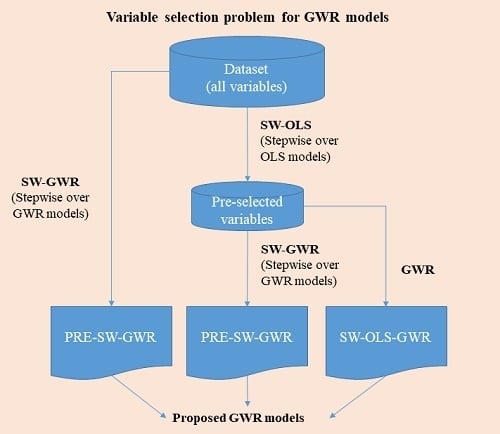
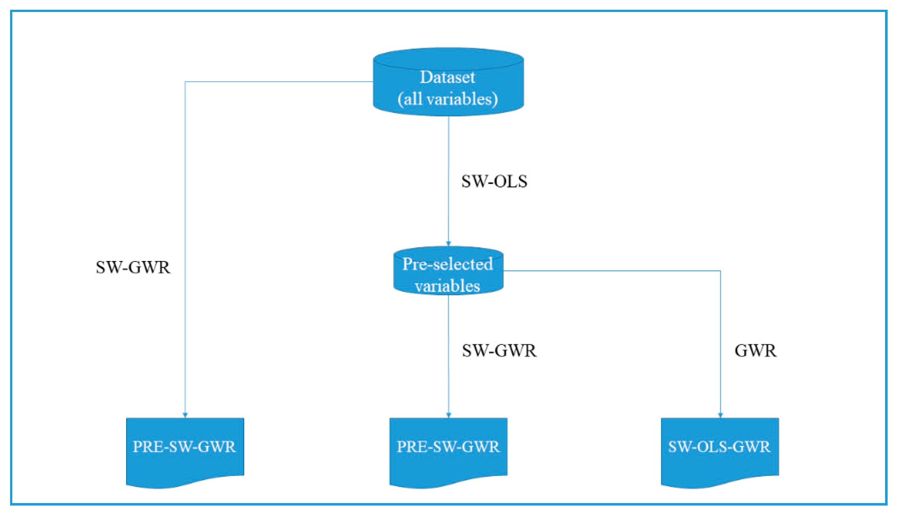
Having into account the considerations above, we propose three alternatives for selecting the best GWR model explaining the rental price: SW-OLS-GWR, Pre-SW-OLS-GWR and SW-GWR. Figure 1 shows a flow chart describing the development of these procedures.

The step-by-step performing of the proposed procedures is detailed below. Computational effort increases from the first to the third suggested alternatives.

SW-OLS-GWR:

Step 1: Obtain the stepwise solution for the OLS regression (SW-OLS) considering all the possible variables.

Step 2: Apply GWR to the model obtained in Step 1.

Pre-SW-OLS-GWR:

Step 1: Obtain the SW-OLS solution considering all the possible variables.

Step 2: Pre-select the best global variables (for instance, select the variables that verify $\Delta F_k^s<MI$ for given MI and s).

Step 3: Apply stepwise procedure for the GWR (SW-GWR) considering the pre-selected variables.

SW-GWR:

Step 1: Apply SW-GWR considering all the variables. Use a stopping rule as $\Delta F_k^s<MI$ for reducing time consumption.

3.3. Data Collection

The case study deals with the Airbnb listings in the island of Gran Canaria. This island is part of the Canary Islands archipelago, Spain (see Figure 2), an important tourist destination in Europe. Although Gran Canaria is well known as a sun and beach tourist destination, the properties offered by Airbnb are not restricted to areas near the coast, but they are distributed throughout the island.

The data was collected from different sources: (a) Airbnb’s listing, to extract the characteristics and locations of the properties; (b) Geographic Information Systems (GIS), to obtain some spatial characteristics of the properties; and (c) Flickr photo repository, to identify the most relevant points of interests in the island through the number of pictures shown in the platform.

The information obtained from Airbnb website was downloaded by January 2018 and is mainly about the characteristics of the properties (number of rooms, beds, other services, etc.), hosts (super-host qualification, language spoken, review counts, etc.) and rental policies (instant booking service, minimum stay length, etc.). A total of 124 variables were extracted from this platform. In order to gather information uniquely for properties currently rented, we decided to choose those having at least one guest review, in a similar way to what had been done in previous studies (i.e., in [10]). Moreover, in order to have a homogenous sample, we decided to select only entire properties, removing from the sample private and shared rooms. Applying these restrictions, the sample was composed of 2259 units.

Some other variables were generated from the spatial location of the accommodation. Specifically, GIS were used to estimate the Euclidean distance from every property to the closest beach. Some new dummy variables were built to show whether the property is in the first, second or third beach line (200, 500 or 1000 m from the closest beach, respectively). To represent the market competition, the number of Airbnb’s listings at a maximum distance of 100, 300 and 500 m were calculated. The distances to the main cities (those with a population over 50,000) and to the ship port and airport were also calculated.

Finally, variables showing the property location with respect to the main point of interests in the destination were calculated. In particular, we use the layer shown in [33] containing 206,897 locations’ pictures uploaded on Flickr in Gran Canaria between 2005 and March 2018. Flickr is a web platform that allows users to upload and share pictures (https://www.flickr.com/). The location of these pictures was interpreted as visitors’ point of interest in the island. The variables counting the number of photos uploaded in a buffer of 500 and 1000 m radius from each property represent how interesting the surroundings of the property are.

A total of 150 explanatory variables were obtained: 124 from Airbnb, 15 from the property locations and one from Flickr. They are described in Appendix A.

4. Results and Discussion

We apply the methodology above to find the determinants of the rental price of the Airbnb listings in Gran Canaria. We consider, as usual (see [14,33], among others), the logarithm of the price as the dependent variable. Then, we apply the different procedures proposed to find the set of variables that best fit the GWR model. We include the adaptive Gaussian kernel in the model and take the AICc as goodness of fit measure for comparing OLS and GWR results.

The direct application of the stepwise algorithm directly on the geographic regression requires the resolution of ${\displaystyle \sum _{i=1}^{T}i}$ GWRs, being T number of the candidate variables (for T = 150 we have 11,325 GWRs) and each one of the GWR regressions requires 2259 OLS regressions. In order to compare results and computational efforts, we apply the three techniques for model selection described above.

4.1. SW-OLS-GWR Procedure

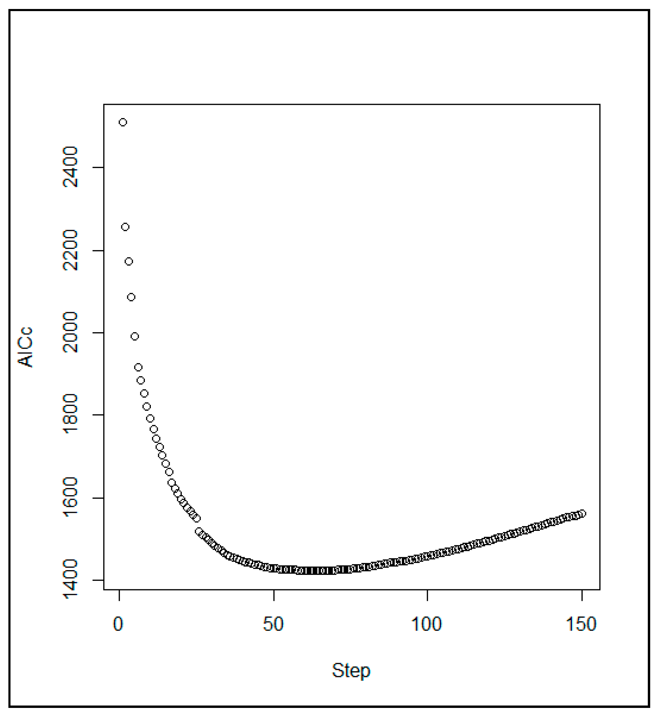
First, we apply the stepwise algorithm in the OLS model over the 150 possible descriptors (SW-OLS). As this procedure can be executed in seconds, a no stopping rule was applied when searching the set of variables that minimize the AICc. Figure 3 shows the algorithm evolution along the different steps. As can be observed, the AICc decreases significantly during the first 37 steps (note that a new variable is added to the model in each step), following a low-steep decrease until step 64 where the AICc starts to grow until using all descriptors. The minimum AICc is 1,422,589 corresponding to the 64-variable model that explains 60.5% of the price variability in the dataset. Nevertheless, having into account the parsimony principle, we selected the first 57 variables entering in the model as candidates of price determinants, as the AICc reduction from this point on is almost insignificant (the reduction of the last seven variables is less than three AICc units). The AICc and the adjusted R² for the 57-variable model were 1425.459 and 0.603, respectively. Appendix A lists the variables following the entry order in the SW-OLS procedure.

Next, the GWR was applied to the 57-variable model obtained from the SW-OLS procedure. The adaptive bandwidth selected in the local version was 800 neighbours (the distance to the 800-th nearest neighbour). The application of the GWR substantially reduced the AICc (1346.583) and the adjusted R² was 0.623, meaning a 2% increase in the dependent variable explanation. The better fitting of the GWR was confirmed by the significance of the L1-Test (p-value = 0.037) and B-Test (p-value = 0.012). The software could not obtain the p-value for the L2-test.

4.2. Pre-SW-GWR Procedure

The SW-GWR algorithm was coded in R using functions contained in the GWmodel package [31,34,35]. This algorithm was executed considering only the first 57 variables obtained from the SW-OLS procedure. Figure 4 shows the AICc in each step of the algorithm performance. The model with the lowest AICc was the one containing 36 variables and the adaptive bandwidth chosen in this case was 225 neighbours. The AICc for this model was 1275.365, meaning a reduction of more than 150 units with respect to the one obtained by SW-OLS and 71.218 units with respect to the SW-OLS-GWR procedure. The adjusted R² was 0.648, a 2.5% higher than achieved with the SW-OLS-GWR procedure. Moreover, the B-Test, L1-Test and L2-Test were significant at 1%, showing that the GWR improved the fit obtained with the global version of this model.

A no stopping rule was imposed (all candidate variables were evaluated). For the sake of comparison,

Table 1. Pre-SW-GWR step-by-step performance.

Step	Variable	AICc	$\mathbf{\Delta }\mathit{A}\mathit{I}\mathit{C}{\mathit{c}}_{}^1$	$\mathbf{\Delta }\mathit{A}\mathit{I}\mathit{C}{\mathit{c}}_{}^2$	$\mathbf{\Delta }\mathit{A}\mathit{I}\mathit{C}{\mathit{c}}_{}^3$	Adj-R2	Bandwidth
1	Bathrooms	1963.745				0.494	42
2	Pool	1790.498	−173.247			0.536	42
3	Bedrooms	1639.400	−151.098	−324.346		0.573	38
4	#Properties	1540.275	−99.125	−250.224	−423.471	0.597	38
5	Dryer	1492.159	−48.116	−147.241	−298.339	0.611	38
6	Dist_Telde	1454.810	−37.349	−85.465	−184.590	0.620	38
7	Cancel_policy	1432.370	−22.440	−59.789	−107.905	0.630	38
8	Hot_tub	1415.896	−16.474	−38.914	−76.263	0.629	47
9	Dist_LPGC	1400.980	−14.916	−31.390	−53.829	0.634	47
10	German	1396.044	−4.937	−19.852	−36.326	0.639	48
11	Essentials	1394.066	−1.978	−6.915	−21.830	0.636	56
12	Air_conditioning	1381.863	−12.203	−14.181	−19.118	0.629	74
13	Beds	1365.200	−16.663	−28.866	−30.844	0.638	69
14	Reviews_count	1354.847	−10.352	−27.016	−39.219	0.642	69
15	Beach500m	1348.687	−6.160	−16.512	−33.175	0.642	74
16	Wireless_Internet	1345.877	−2.810	−8.970	−19.323	0.643	79
17	TV	1338.540	−7.336	−10.147	−16.307	0.647	79
18	Dist_Airp	1333.869	−4.672	−12.008	−14.818	0.649	81
19	Comp500m	1328.440	−5.429	−10.101	−17.437	0.646	92
20	Elevator	1324.574	−3.865	−9.294	−13.966	0.643	109
21	French	1319.847	−4.728	−8.593	−14.022	0.646	109
22	Beach200m	1313.561	−6.285	−11.013	−14.878	0.645	117
23	Is_superhost	1309.226	−4.335	−10.621	−15.348	0.645	128
24	Extra_pillows	1307.198	−2.028	−6.363	−12.649	0.646	131
25	Cable_TV	1302.679	−4.519	−6.547	−10.882	0.648	134
26	Hair_dryer	1301.445	−1.234	−5.753	−7.781	0.650	134
27	Kitchen	1300.534	−0.911	−2.145	−6.664	0.651	134
28	Dishwasher	1300.041	−0.493	−1.404	−2.638	0.640	202
29	Security_deposit	1294.207	−5.833	−6.327	−7.238	0.641	206
30	Cooking_basics	1289.985	−4.222	−10.055	−10.549	0.643	206
31	Family_kid_friendly	1286.977	−3.008	−7.230	−13.064	0.644	206
32	Smoking_allowed	1282.972	−4.005	−7.014	−11.236	0.646	206
33	BBQ_grill	1279.484	−3.488	−7.493	−10.501	0.647	206
34	Exp_guest+Govid	1276.782	−2.702	−6.190	−10.195	0.649	206
35	Polish	1276.108	−0.674	−3.376	−6.864	0.650	206
36	Pict_500m	1275.365	−0.743	−1.417	−4.119	0.648	225

shows the composition of the models if a stopping rule of type $\Delta AIC{c}_{}^s>-3$ was considered (a minimum reduction of three AICc units after s steps). If this minimum reduction is applied after only one step (see column $\Delta AIC{c}_{}^1$), the model includes the first 23 variables. A two-step delay (see column $\Delta AIC{c}_{}^2$) would only add three new variables. The $\Delta AIC{c}_{}^3$ increment rule would stop the algorithm performance with 36 variables. The maximum adjusted R² (0.648) was obtained for the model with the last stopping rule. The inclusion of variables 35 and 36 originated an AICc decrease of only 1.417 units and a small reduction in adjusted R² (column 7 in Table 1) that does not support their inclusion in the model.

The last column in Table 1 shows the bandwidth selected in each step of the Pre-SW-GWR. These bandwidths vary from 38 to 225 neighbourhoods, showing an increasing trend when new variables are included in the model.

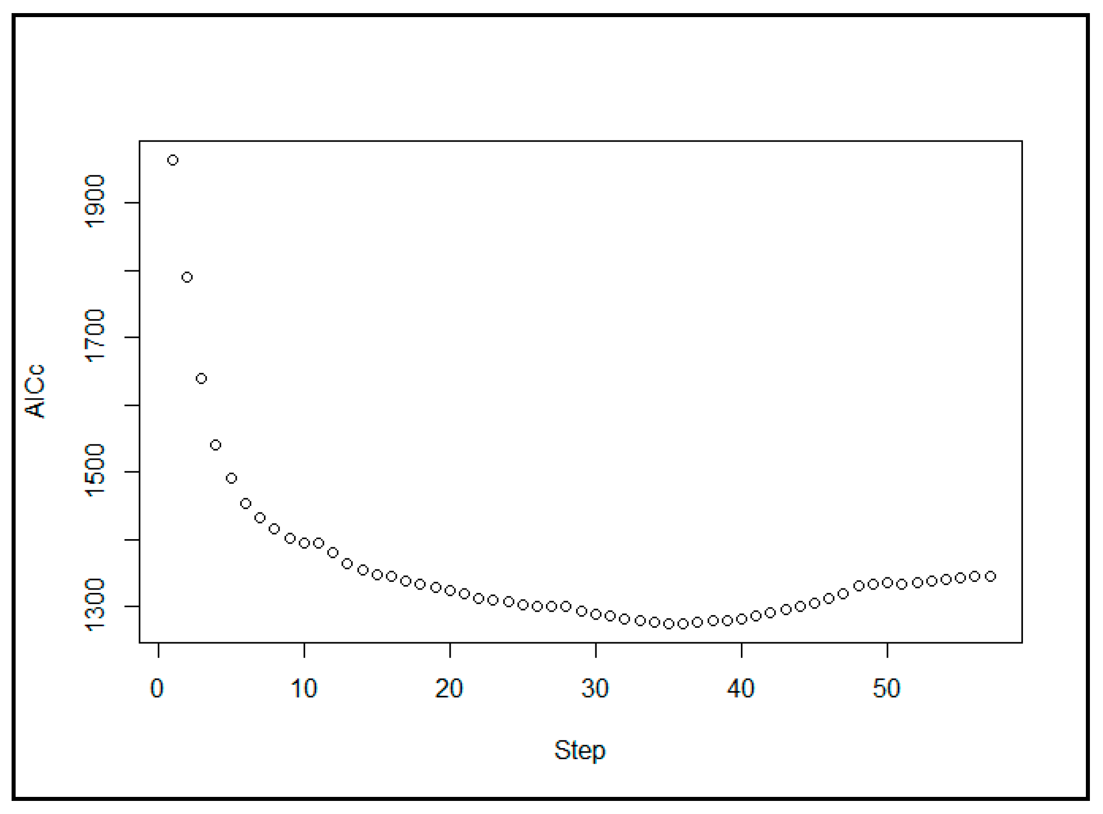
4.3. SW-GWR Procedure

Finally, the stepwise procedure was performed directly on the GWR without pre-selecting variables, that is, considering the 150 variables. The selected model was obtained in step 40 with an AICc of 1219.692. This solution implies a reduction of more than 55 AICc units with respect to the obtained by the Pre-SW-GWR, and a 1.5% increase in adjusted R². Again, B-test, L1-test and the L2-test were significant at 1%, which means that the fit of the local version of this model is better than the global one.

Table 2. SW-GWR step-by-step performance.

Step	Variable	AICc	$\mathbf{\Delta }\mathit{A}\mathit{I}\mathit{C}{\mathit{c}}_{}^1$	$\mathbf{\Delta }\mathit{A}\mathit{I}\mathit{C}{\mathit{c}}_{}^3$	$\mathbf{\Delta }\mathit{A}\mathit{I}\mathit{C}{\mathit{c}}_{}^3$	Adj-R2	Bandwidth
1	Bathrooms	1963.746				0.494	42
2	Pool	1790.498	−173.247			0.536	42
3	Bedrooms	1642.354	−148.144	−321.392		0.572	39
4	#Properties	1542.882	−99.472	−247.616	−420.864	0.596	39
5	Pict_1km	1493.958	−48.925	−148.397	−296.541	0.609	38
6	Dryer	1445.602	−48.356	−97.281	−196.753	0.621	40
7	Suitable_for_events	1410.584	−35.017	−83.373	−132.298	0.633	39
8	Beds	1399.254	−11.330	−46.348	−94.704	0.640	39
9	Dist_beach	1391.136	−8.118	−19.448	−54.466	0.645	39
10	Cancel_policy	1384.210	−6.926	−15.044	−26.374	0.653	39
11	Essentials	1380.696	−3.514	−10.440	−18.558	0.640	56
12	Air_conditioning	1364.979	−15.717	−19.231	−26.157	0.635	69
13	Dist_Airp	1346.458	−18.521	−34.238	−37.752	0.640	70
14	French	1334.715	−11.743	−30.264	−45.981	0.645	69
15	Reviews_count	1319.490	−15.225	−26.968	−45.488	0.650	69
16	Hot_tub	1315.907	−3.584	−18.808	−30.551	0.654	69
17	Indoor_fireplace	1310.376	−5.531	−9.114	−24.339	0.657	69
18	Beach500m	1307.830	−2.546	−8.077	−11.660	0.654	77
19	Elevator	1304.841	−2.989	−5.535	−11.066	0.657	77
20	Bed_linens	1304.117	−0.725	−3.714	−6.260	0.649	103
21	Smoke_detector	1295.905	−8.212	−8.937	−11.926	0.650	109
22	Dist_LPGC	1289.917	−5.988	−14.200	−14.924	0.652	109
23	Comp500	1285.087	−4.830	−10.818	−19.030	0.656	105
24	TV	1281.761	−3.325	−8.156	−14.143	0.654	117
25	Breakfast	1274.378	−7.383	−10.709	−15.539	0.647	165
26	Beach201_500	1266.657	−7.721	−15.104	−18.430	0.648	169
27	Dishwasher	1260.417	−6.241	−13.961	−21.345	0.650	169
28	Is_superhost	1253.886	−6.530	−12.771	−20.492	0.650	180
29	German	1247.034	−6.853	−13.383	−19.623	0.652	180
30	Dist_Telde	1242.425	−4.609	−11.461	−17.991	0.654	180
31	Hair_dryer	1238.286	−4.139	−8.747	−15.600	0.655	180
32	Security_deposit	1235.656	−2.631	−6.769	−11.378	0.657	180
33	Exp_guest+Govid	1232.561	−3.095	−5.725	−9.864	0.657	179
34	Lockbox	1229.881	−2.680	−5.775	−8.405	0.660	180
35	Cooking_basics	1227.535	−2.346	−5.026	−8.120	0.657	207
36	Refrigerator	1225.316	−2.219	−4.565	−7.245	0.658	207
37	Beach1000m	1223.183	−2.133	−4.352	−6.698	0.660	204
38	Polish	1222.020	−1.163	−3.296	−5.515	0.661	202
39	Kitchen	1220.408	−1.612	−2.775	−4.908	0.662	202
40	Spanish	1219.692	−0.716	−2.328	−3.491	0.663	206

shows the variables included in the best model by entry order. The table also presents the different AICc increments when applying the stopping rule $\Delta AIC{c}_{}^s>-3$, with s = 1, 2 or 3. In this case, the number of variables in the model goes from 33 (one-step increment) to 40 (three-step increment). The stopping rule with s = 1 resulted a 17-variable model. However, unlike with Pre-SW-GWR, s = 2 and s = 3 led to a very similar pattern (38 and 40 variables, respectively).

4.4. Comparing the Three Procedures

Table 3. Comparison between the three methods used for selecting variables.

	SW-OLS	SW-OLS-GWR	Pre-SW-GWR	SW-GWR
#Variables	57	57	36	40
Bandwidth	2259	800	225	206
AICc	1425.459	1346.583	1275.365	1219.692
Adjusted R2	0.603	0.623	0.648	0.663
Adjusted α	0.05	0.0191	0.0066	0.0063
Average significant variables	50	25.854	12.021	12.549
Min. significant variables	50	15	2	2
Max. significant variables	50	41	33	28
IQR significant variables	0	14	12	13
#OLS solved models	11,325	13,584	3,259,737	12,040,470

shows a summary of the results obtained with the three methods. The results for the Pre-SW-GWR and SW-OLS procedures are those obtained by applying the stopping rule $\Delta AIC{c}_{}^3>-3$.

In order to compare the complexity of the different procedures, the last row in Table 3 shows the number of OLS models executed to reach the solution by each procedure. The larger the complexity, the better the model is. The SW-OLS procedure is a global regression and incurs in the worst fit indexes. This model obtained an AICc of 1425.459 and explained 60.3% of the price variability in the dataset. The fit substantially improved by converting the SW-OLS solution to a local model applying GWR (SW-OLS-GWR), reducing the AICc by 78.876 units and increasing the model explanation by 2%. The algorithm complexity increases by 16.6% with this conversion.

Obviously, directly working on GWR models significantly increases the computational effort. In return, better adjustments were obtained. When the SW was executed using GWR considering only the most influential variables in the global model (Pre-SW-GWR), a substantial improvement with respect to the SW-OLS-GWR was achieved, reducing 71.218 AICc units and increasing the adjusted R² by 2.5%. The pre-selection of variables reduced by 62% the candidate variables, with the consequent reduction in computational cost. Although the first two variables selected by Pre-SW-GWR procedure coincided with those chosen by SW-OLS, the order no longer matches. In fact, the sixth variable to enter in the Pre-SW-GWR model is the 26th in the SW-OLS solution. Moreover, the Pre-SW-GWR procedure provided a shorter model than the selected one by the SW-OLS procedure, reducing the number of variables by 21.

The last alternative (SW-GWR) improved the adjustments obtained by the other techniques (a 55.673 AICc units reduction and increasing the adjusted R² by 1% with respect to Pre-SW-GWR). Nevertheless, the computation times increased significantly (3.69 times the one employed by Pre-SW-GWR).

Although the number of variables containing the best models using Pre-SW-GWR and SW-GWR procedures was quite similar, there were differences in relation to the specific variables included in each one of them. In particular, the SW-GWR procedure considered 10 (out of 40) variables that were not pre-selected by the SW-OLS procedure. For instance, Pict_1km (pictures in 1 km from the property) entered in the SW-GWR model in step 5, providing a reduction of 48.925 AICc units with respect to the previous model. Nevertheless, this factor was only considered by SW-OLS procedure from step 90. Consequently, the most influential variables globally do not necessary have to be influential locally as well (and vice versa).

The bandwidths considered by the different processes varied from 206 to 800. This variability makes it impractical to preselect this parameter prior to the execution of a SW procedure, as required by the function implemented for this purpose in the GWmodel R package.

When the GWR is performed, the significance level for the coefficients must take into account the dependence of the subsamples. The fifth row in Table 3 shows the adjusted α (equivalent to a 5% ordinary significance level) considered for the different models. Rows 7 to 10 in Table 3 describe the number of significant variables for the different cases. A total of 50 variables were significant for the SW-OLS procedure, but the number of significant factors for GWR models varied according to the location of the property. The solution when applying the SW-OLS-GWR procedure included higher average number of significant variables than those obtained by applying the Pre-SW-GWR and SW-GWR procedures.

4.5. Results with GWR

In general, the most relevant determinants found in Table 1 and Table 2 confirm findings of previous studies. Some of the structural attributes of the property (number or bathrooms and beds), host professionalism, as indicated by the number of properties managed, and spatial factors are commonly observed as price determinants in other destinations [2,10,13,14]. Some new structural attributes are found here, such as the existence of a dryer and suitability of events, which it is related to the specific conditions and type of lodgings (full house) analysed here. Moreover, in general, the coefficient signs are as expected, i.e., additional services and uploaded photos have a positive influence while variables associated with distance and competition have a negative impact.

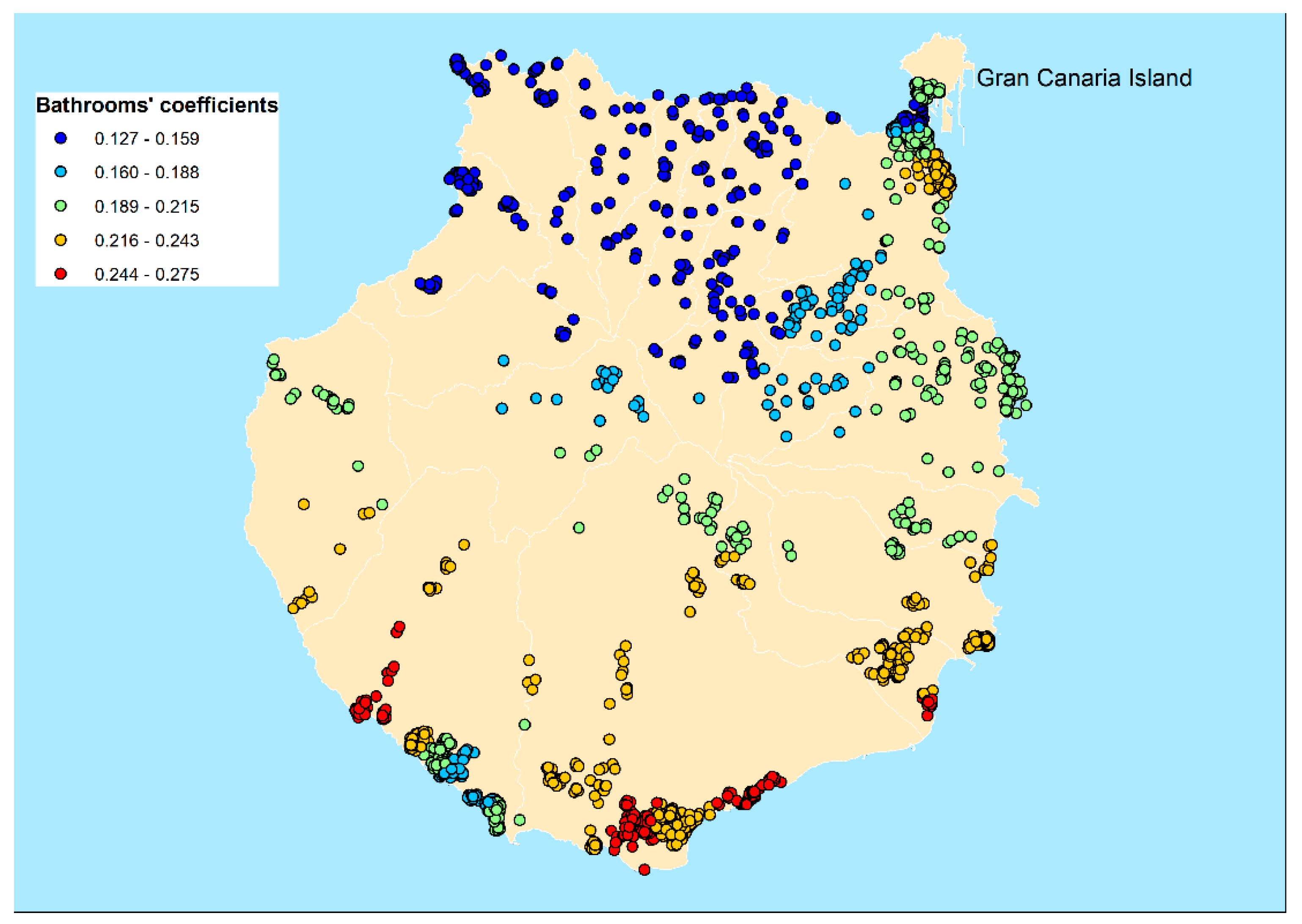
In addition to the overall improvement in model fit, the GWR model also allows evaluating the spatial effect of each characteristic. The solution obtained through the proposed procedures can be easily exported to a GIS for spatial analysis. As an example, Figure 5 shows the spatial distribution for the Bathrooms’ coefficients when the SW-GWR procedure was applied. The results reveal that the price increase due to an additional bathroom varies between 12.7 and 27.5%, being 20.1% the average increase. Note that this increase is fixed to 21.7% for the whole sample when applying an OLS model. The green/orange dots in Figure 5 show properties with coefficients close to the OLS coefficient. As it can be observed, the effect of an additional bathroom in certain southern areas is clearly above average whereas it is below average in the northwest. This information can be used by hosts when setting the rental price of a property according to the number of bathrooms and location.

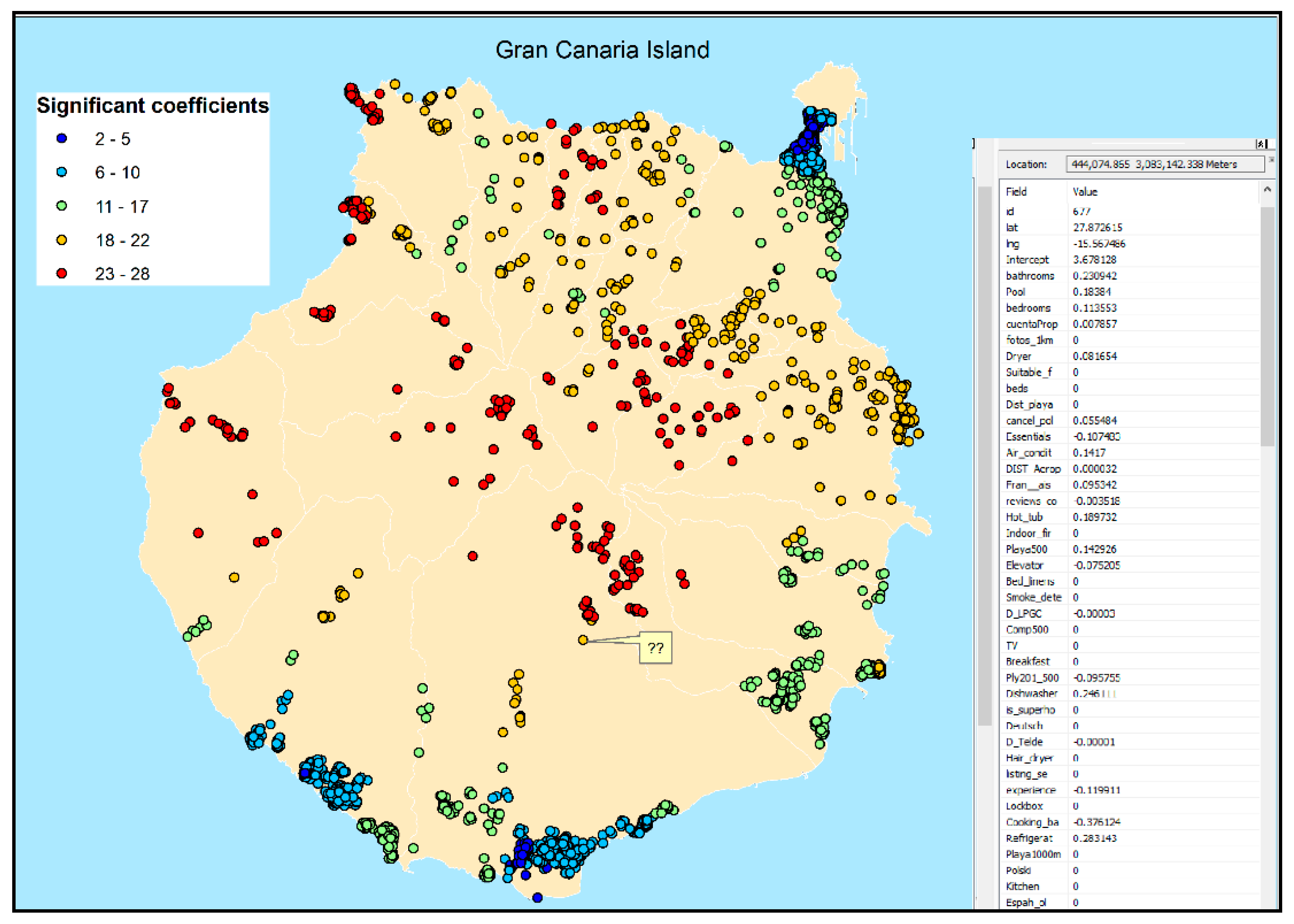
Although the SW-GWR model contains 40 variables, they are not significant for every property. Figure 6 shows the distribution of the number of significant coefficients in the sample. The number of local factors explaining the rental price varies between 2 and 28. On the right hand side of the map, it is shown the estimated coefficients of the pointed property (0 must be interpreted as non-significant coefficient).

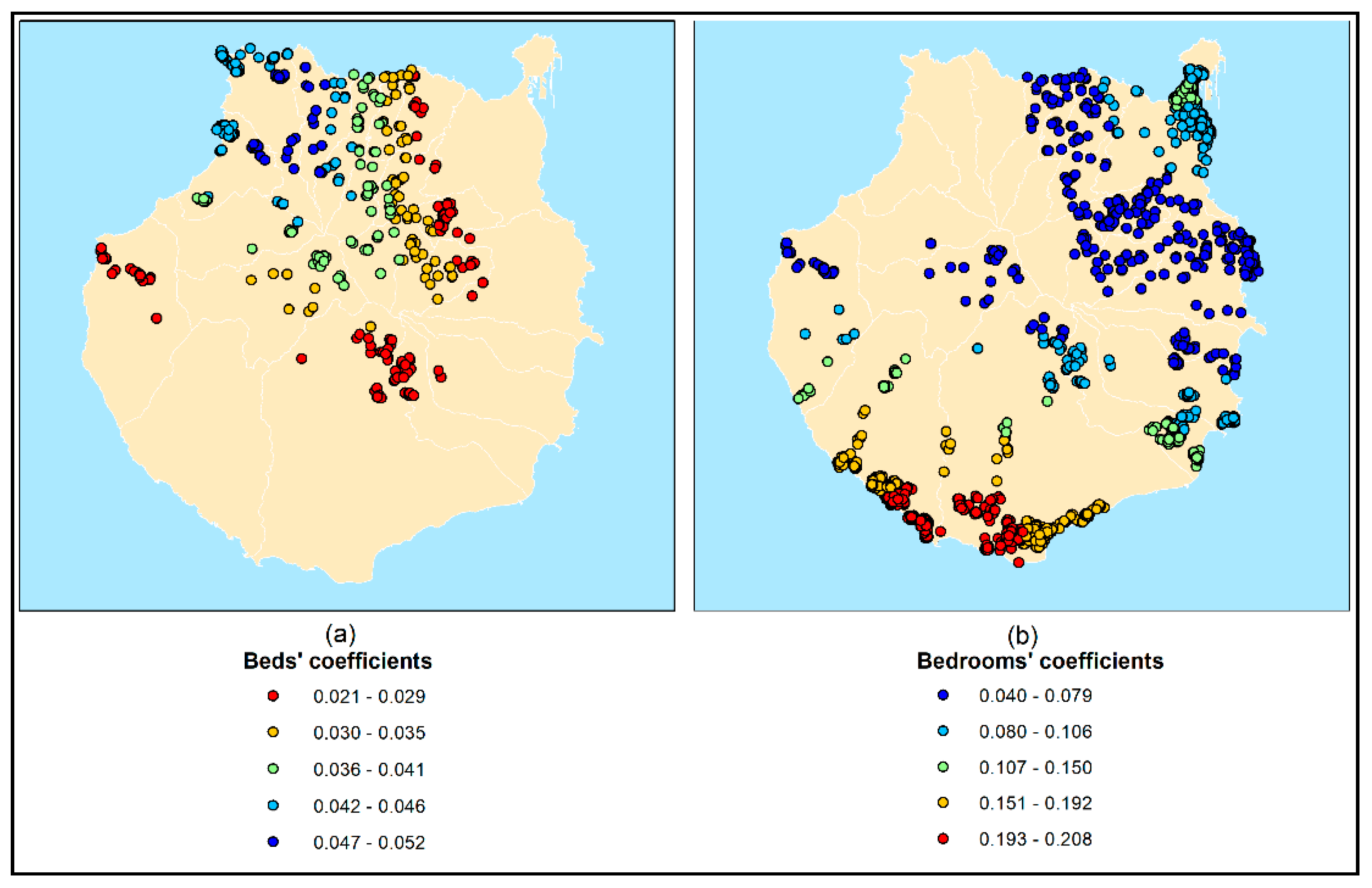
To illustrate how the GWR discriminates between the effects of alternative factors, Figure 7 shows the coefficient of the significant local variables Beds (a) and Bedrooms (b). Although the effect of these two variables is constant and significant for the whole sample using the OLS model, they are not simultaneously significant in many properties when applying the GWR model. Moreover, when only one of these variables is significant, the value of the coefficient is usually medium–high. Nevertheless, when both variables are significant (228 properties out of 2259), the coefficients have lower values. This result shows that both factors represent substitutable effects in the area.

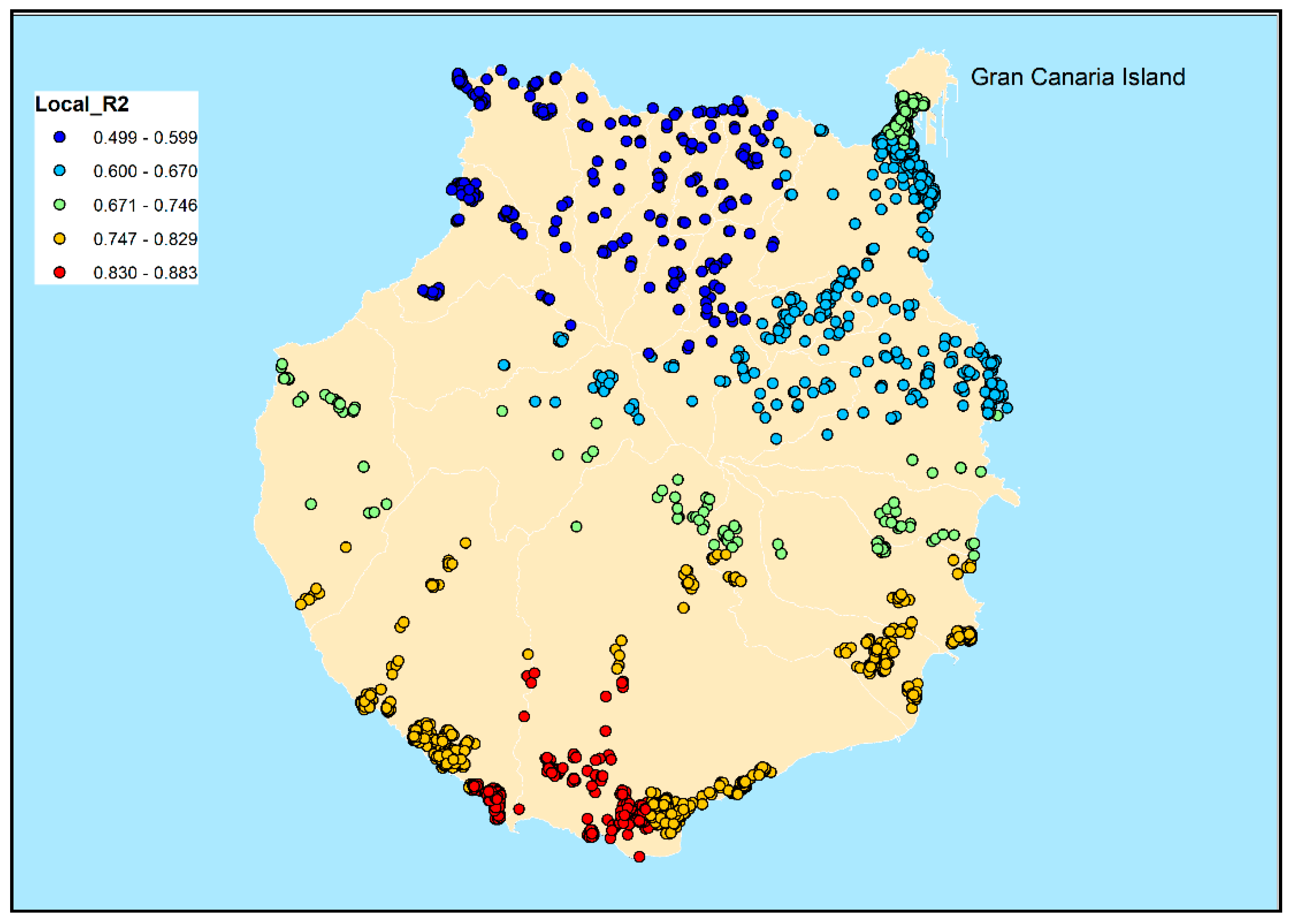
Finally, Figure 8 shows the distribution of the local R² across the island. The model works pretty well in the south (with local R² above 0.747), worsening as we move northwest. This result suggests that the information collected is sufficient to characterize the rental price in the south, but in the northwest there are specific characteristics of the area that have not been captured by the model.

5. Conclusions and New Working Lines

Nowadays, analysing price determinants in P2P accommodation units involves many variables. Some of them are shown in digital platforms and others are related to the location of the property. Therefore, the methods to find out those significant factors and their quantitative influence on price must deal with the reality of high number of variables and spatial effects.

This paper proposes GWR models to explain prices in the P2P accommodation market. This type of regression allows estimating the effect of the regressors locally, in other words, the coefficients of the regression are estimated for each property. This method has two significant advantages: On the one hand, it is possible to estimate the effect of the same variable in different locations. On the other hand, it is possible to discriminate significant variables according to the area where the property is located. By these means, the location characteristics influencing the price can be identified.

Studies on selection of variables for GWR models are scant and have never been applied, to our knowledge, on databases with many variables (above 100). In this regard, the methods presented in this paper are useful for social researchers that look for finding the price determinant estimation model that best fit the data. Different procedures to find suitable GWR models have been proposed in this paper: Obtain a good global solution (SW-OLS) and then convert it to local by means of GWR (SW-OLS-GWR); Pre-select good global variables and apply a SW procedure considering these variables (Pre-SW-GWR); and apply SW to GWR taking all the variables as candidates (SW-GWR).

For the case study, the best fit is achieved with the SW-GWR procedure, followed by the Pre-SW-OLS-GWR and the SW-OLS-GWR procedures, with significant differences between them. However, the better the fit, the greater the computational effort required. In order to reduce the computational effort, a stopping rule was proposed. The most robust solution among the analysed options is to stop the procedure when the accumulated reduction in AICc after three steps is less than three units.

The SW-OLS-GWR is the most common procedure in the application of GWR models when there are many possible regressors. However, as shown in the case study, a good solution for the OLS model is not necessarily a good solution for the GWR model as well. Furthermore, preselecting a set of suitable global variables does not ensure that the best solution will be reached, as the SW-GWR procedure can take variables that are not part of this set. However, the preselecting procedure is faster than applying GWR over the whole sample and variables. On the other hand, procedures to select variables in which the bandwidth is fixed a priori are not recommendable because the bandwidth depends on the variables that make up the GWR model.

The methodology presents some limitations. As it was observed in the case study, the process employed in the selection of variables can be highly time-consuming, so it would be interesting to investigate methods to reduce running times. It would also be interesting to add other functionalities to the procedure in order to avoid collinearity problems or discard non-influential factors.

References

- Bakker, M.; Twining-Ward, L. Tourism and the Sharing Economy; World Bank: Washington, DC, USA, 2018. [Google Scholar]
- Gibbs, C.; Guttentag, D.; Gretzel, U.; Morton, J.; Goodwill, A. Pricing in the sharing economy: A hedonic pricing model applied to Airbnb listings. J. Travel Tour. Mark. 2017, 12, 1–11. [Google Scholar] [CrossRef]
- Espinet, J.M.; Sáez, M.; Coenders, G.; Fluvià, M. Effect on prices of the attributes of holiday hotels: A hedonic prices approach. Tour. Econ. 2003, 9, 165–177. [Google Scholar] [CrossRef]
- Thrane, C. Hedonic Price Models and Sun-and-Beach Package Tours: The Norwegian Case. J. Travel Res. 2005, 43, 302–308. [Google Scholar] [CrossRef]
- Ert, E.; Fleischer, A.; Magen, N. Trust and reputation in the sharing economy: The role of personal photos in Airbnb. Tour. Manag. 2016, 55, 62–73. [Google Scholar] [CrossRef]
- Chen, Y.; Xie, K. Consumer valuation of Airbnb listings: A hedonic pricing approach. Int. J. Contemp. Hosp. Manag. 2017, 29, 2405–2424. [Google Scholar] [CrossRef]
- Benítez-Aurioles, B. Why are flexible booking policies priced negatively? Tour. Manag. 2018, 67, 312–325. [Google Scholar] [CrossRef]
- Lorde, T.; Jacob, J.; Weekes, Q. Price-setting behavior in a tourism sharing economy accommodation market: A hedonic price analysis of AirBnB hosts in the caribbean. Tour. Manag. Perspect. 2019, 30, 251–261. [Google Scholar] [CrossRef] [Green Version]
- Teubner, T.; Hawlitschek, F.; Dann, D. Price determinants on Airbnb: How reputation pays off in the sharing economy. J. Self-Gov. Manag. Econ. 2017, 5, 53–80. [Google Scholar]
- Wang, D.; Nicolau, J.L. Price determinants of sharing economy based accommodation rental: A study of listings from 33 cities on Airbnb.com. Int. J. Hosp. Manag. 2017, 62, 120–131. [Google Scholar] [CrossRef] [Green Version]
- Tang, L.; Kim, J.; Wang, X. Estimating spatial effects on peer-to-peer accommodation prices: Towards an innovative hedonic model approach. Int. J. Hosp. Manag. 2019, 81, 43–53. [Google Scholar] [CrossRef]
- Önder, I.; Weismayer, C.; Gunter, U. Spatial price dependencies between the traditional accommodation sector and the sharing economy. Tour. Econ. 2018, 25, 1150–1166. [Google Scholar] [CrossRef]
- Sanchez, R.P.; Estrada, L.S.; Marti, P.; Mora-Garcia, R.-T. The What, Where, and Why of Airbnb Price Determinants. Sustainability 2018, 10, 4596. [Google Scholar] [CrossRef] [Green Version]
- Chica-Olmo, J.; González-Morales, J.G.; Zafra-Gómez, J.L. Effects of location on Airbnb apartment pricing in Málaga. Tour. Manag. 2020, 77, 103981. [Google Scholar] [CrossRef]
- Chattopadhyay, M.; Mitra, S.K. Do airbnb host listing attributes influence room pricing homogenously? Int. J. Hosp. Manag. 2019, 81, 54–64. [Google Scholar] [CrossRef]
- Brunsdon, C.; Fotheringham, A.S.; Charlton, M.E. Geographically Weighted Regression: A Method for Exploring Spatial Nonstationarity. Geogr. Anal. 2010, 28, 281–298. [Google Scholar] [CrossRef]
- Fotheringham, S.; Charlton, M.; Brunsdon, C. The Geography of Parameter Space. Class. IJGIS 2006, 10, 297–325. [Google Scholar] [CrossRef]
- Fotheringham, A.S.; Charlton, M.; Brunsdon, C. Two techniques for exploring non-stationarity in geographical data. Geogr. Syst. 1997, 4, 59–82. [Google Scholar]
- Lu, B.; Charlton, M.; Fotheringhama, A.S. Geographically Weighted Regression Using a Non-Euclidean Distance Metric with a Study on London House Price Data. Procedia Environ. Sci. 2011, 7, 92–97. [Google Scholar] [CrossRef] [Green Version]
- Kim, J.; Jang, S.; Kang, S.; Kim, S. (James) Why are hotel room prices different? Exploring spatially varying relationships between room price and hotel attributes. J. Bus. Res. 2020, 107, 118–129. [Google Scholar] [CrossRef]
- Hernández, J.M.; Suárez-Vega, R.; Santana, Y. The inter-relationship between rural and mass tourism: The case of Catalonia, Spain. Tour. Manag. 2016, 54, 43–57. [Google Scholar] [CrossRef]
- Zhang, Z.; Chen, R.J.C.; Han, L.D.; Yang, L. Key Factors Affecting the Price of Airbnb Listings: A Geographically Weighted Approach. Sustainability 2017, 9, 1635. [Google Scholar] [CrossRef] [Green Version]
- Hocking, A.R.R. The Analysis and Selection of Variables in Linear Regression Published by: International Biometric Society Stable URL: http://0-www-jstor-org.brum.beds.ac.uk/stable/2529336. Biometrics 1976, 32, 1–49. [Google Scholar] [CrossRef]
- Suárez-Vega, R.; Acosta-González, E.; Casimiro-Reina, L.; Hernández, J.M. Assessing the Spatial and Environmental Characteristics of Rural Tourism Lodging Units Using a Geographical Weighted Regression Model. In Quantitative Methods in Tourism Economics; Springer Science and Business Media LLC: Berlin, Germany, 2012; pp. 195–212. [Google Scholar]
- Fotheringham, A.S.; Kelly, M.; Charlton, M. The demographic impacts of the Irish famine: Towards a greater geographical understanding. Trans. Inst. Br. Geogr. 2012, 38, 221–237. [Google Scholar] [CrossRef]
- Páez, A.; Uchida, T.; Miyamoto, K. A General Framework for Estimation and Inference of Geographically Weighted Regression Models: 2. Spatial Association and Model Specification Tests. Environ. Plan. A Econ. Space 2002, 34, 883–904. [Google Scholar] [CrossRef]
- Páez, A.; Uchida, T.; Miyamoto, K. A General Framework for Estimation and Inference of Geographically Weighted Regression Models: 1. Location-Specific Kernel Bandwidths and a Test for Locational Heterogeneity. Environ. Plan. A Econ. Space 2002, 34, 733–754. [Google Scholar] [CrossRef]
- Da Silva, A.R.; Fotheringham, A.S. The Multiple Testing Issue in Geographically Weighted Regression. Geogr. Anal. 2015, 48, 233–247. [Google Scholar] [CrossRef]
- Brunsdon, C.; Fotheringham, A.S.; Charlton, M. Some Notes on Parametric Significance Tests for Geographically Weighted Regression. J. Reg. Sci. 1999, 39, 497–524. [Google Scholar] [CrossRef]
- Leung, Y.; Mei, C.-L.; Zhang, W.-X. Statistical Tests for Spatial Nonstationarity Based on the Geographically Weighted Regression Model. Environ. Plan. A Econ. Space 2000, 32, 9–32. [Google Scholar] [CrossRef]
- Gollini, I.; Lu, B.; Charlton, M.; Brunsdon, C.; Harris, P. GWmodel: An R Package for Exploring Spatial Heterogeneity Using Geographically Weighted Models. J. Stat. Softw. 2015, 63, 1–50. [Google Scholar] [CrossRef] [Green Version]
- Wang, M.; Wright, J.; Brownlee, A.; Buswell, R. A comparison of approaches to stepwise regression on variables sensitivities in building simulation and analysis. Energy Build. 2016, 127, 313–326. [Google Scholar] [CrossRef] [Green Version]
- Eugenio-Martin, J.L.; Cazorla-Artiles, J.M.; González-Martel, C. On the determinants of Airbnb location and its spatial distribution. Tour. Econ. 2019, 25, 1224–1244. [Google Scholar] [CrossRef] [Green Version]
- Cai, Y.; Zhou, Y.; Ma, J.; Scott, N. Price Determinants of Airbnb Listings: Evidence from Hong Kong. Tour. Anal. 2019, 24, 227–242. [Google Scholar] [CrossRef]
- Lu, B.; Harris, P.; Charlton, M.; Brunsdon, C. The GWmodel R package: Further topics for exploring spatial heterogeneity using geographically weighted models. Geo. Spat. Inf. Sci. 2014, 17, 85–101. [Google Scholar] [CrossRef]
Figure 1.
Steps for performing the three model selection procedures.
Figure 2.
Gran Canaria Island scenario.
Figure 3.
Stepwise-ordinary least squares (SW-OLS) Akaike Information Criterion (AICc) performance.
Figure 4.
Evolution of the AICc along the Pre-SW-GWR algorithm.
Figure 5.
Distribution of the significant coefficients for the variable Bathrooms (SW-GWR model).
Figure 6.
Number of significant local variables for every property (SW-GWR model).
Figure 7.
Significant coefficients for Beds and Bedrooms (SW-GWR model).
Figure 8.
Local R2 distribution (SW-GWR model).