Household Level Vulnerability Analysis—Index and Fuzzy Based Methods


Faculty of Civil Engineering, Architecture and Geodesy, University of Split, Matice hrvatske 15, 21000 Split, Croatia
ISPRS Int. J. Geo-Inf. 2020, 9(4), 263; https://0-doi-org.brum.beds.ac.uk/10.3390/ijgi9040263
Submission received: 31 January 2020
/
Revised: 8 April 2020
/
Accepted: 17 April 2020
/
Published: 19 April 2020
(This article belongs to the Special Issue GI for Disaster Management)
Abstract
:Coastal vulnerability assessment due to climate change impacts, particularly for sea level rise, has become an essential part of coastal management all over the world. For the planning and implementation of adaptation measures at the household level, large-scale analysis is necessary. The main aim of this research is to investigate and propose a simple and viable assessment method that includes three key geospatial parameters: elevation, distance to coastline, and building footprint area. Two methods are proposed—one based on the Index method and another on fuzzy logic. While the former method standardizes the quantitative parameters to unit-less vulnerability sub-indices using functions (avoiding crisp classification) and summarizes them, the latter method turns quantitative parameters into linguistic variables and further implements fuzzy logic. For comparison purposes, a third method is considered: the existing Index method using crisp values for vulnerability sub-indices. All three methods were implemented, and the results show significant differences in their vulnerability assessments. A discussion on the advantages and disadvantages led to the following conclusion: although the fuzzy logic method satisfies almost all the requirements, a less complex method based on functions can be applied and still yields significant improvement.
1. Introduction
At present, the assessment of coastal vulnerability due to climate change impacts is an essential input for coastal management processes all over the world [1]. The impact of sea level rise is the main climate impact taken into account when managing coastal areas, from determining future use to planning adaptation measures [1,2,3]. The term “vulnerability” is a function of hazard characteristics, the sensitivity of the assets exposed, and adaptive capacity, which all vary by time and depend on contexts such as socio–economic factors [2]. Hazard characteristics define the exposure of the system to phenomena, sensitivity describes how the system is affected, and adaptive capacity defines the system’s ability to maintain its functions. For example, in the case of a flood, the hazard characteristics are water depth and velocity; sensitivity is represented by the number of people and assets flooded; and adaptive capacity is the capacity of emergency infrastructure and flood defence structures. In this paper, “vulnerability” refers to physical vulnerability, as described above, from the perspectives of disaster management, climate change, and other related aspects [4]. Sociology and economics refer to “social vulnerability”, which focuses on identifying the most vulnerable groups of people and examines social factors and economic assets, such as poverty, access to food and housing, and human and social capital [4,5]. A vulnerability assessment could follow a quantitative approach based on related indicators and indices, or a qualitative approach based on the perspectives of stakeholders [6]. In this paper, a quantitative approach based on indices is used.
Vulnerability requires assessment methods that apply to different scales: spatial (large, medium, and small), temporal (short, mid, and long term), and management (local, regional, and national) [1]. While assessments used at the national or regional level identify the most vulnerable areas and help in prioritizing measures (scales in the range of 1:100.000 to 1:25.000), large-scale assessments are necessary for the planning and implementation of adaptation measures at the household level [3,7]. An overview of the methods for assessing coastal vulnerability is given in [1]. These methods are classified into four categories: Index-based methods, Indicator-based approaches, GIS-based decision support systems, and methods based on dynamic computer models.
Index-based and Indicator-based methods differ in the methodological approaches they use for the definition of indices/indicators, but are similar in their quantification and combination of indices/indicators in a single parameter describing vulnerability.
Index-based methods calculate the vulnerability index (unit-less value) by summarizing sub-indices (values of selected parameters) [8,9]. This method is widely recognised and has several variants, such as the coastal vulnerability index for sea level rise [10], the composite vulnerability index [11], and the multi-scale coastal vulnerability index [12]. Index-based methods start with a selection of key parameters that represent the processes or assets of importance for coastal vulnerability. The physical parameters include geomorphology, shoreline change rates, coastal slope, rate of sea level rise, wave heights, tidal range, and proximity to coast. The human influence parameters are river regulation, engineered frontage, land use, coastal protection structures, etc. The socio–economic parameters are the affected population, the affected cultural heritage, the affected infrastructure, etc. The second step quantifies the contribution of the selected key parameters to coastal vulnerability using indices from 1 to 5, where 1 indicates a low contribution to coastal vulnerability, and 5 indicates a high contribution to coastal vulnerability. Experts have developed classification schemas, where the key parameter values are classified by the values of the sub-indices. For example, a sea level rise with a rate of less the 1 mm/year is classified as value 1 for the sub-index, that with a rate of 1–2 mm/year is given value 2, that with a rate of 2–5 mm/year is value 3, that with a rate of 5–7 mm/year is value 4, and that with a rate of 7 mm/year and over is value 5 [1]. The final step integrates the sub-indices into a single index via the use of selected formulas, such as the product mean or average sum. Additional refinements could be done by using weights for the sub-indices. Index-based methods are used for various scales, from the small scales used at the national level to the large-scales used at the local level.
Indicator-based approaches use indicators representing coastal vulnerability factors, such as sea level rises; extreme weather conditions; coastal erosion and accretion; and the natural, human, and economic assets at risk. Indicators are defined and quantified primarily to measure the progress towards sustainable development, and to guide decision makers in managing coastal areas. Thus, these indicators differ from the indices used by Index-based methods that focus on vulnerability. Similar to Index-based methods, the indicators can be further classified according to their contribution to coastal vulnerability and integrated into a single indicator of vulnerability. For example, the Deduce Interreg project developed a set of 27 core indicators for sustainable coastal zone development [13]. Three indicators addressed climate change vulnerability—(i) sea level rise and extreme weather conditions (quantified by the number of stormy days, the sea level rise, and the length of the protected coastline); (ii) coastal erosion and accretion (quantified by the length of the dynamic coastline, the area and volume of sand nourishment, and the number of people living in the coastal flooding areas); and (iii) the natural, human, and economic assets at risk (quantified by the areas of the protected sites and by the economic values of the assets in the coastal flooding areas). Indicator-based approaches are used for national, regional, and local level assessments.
More complex methods, such as GIS-based decision support systems or dynamic computer models, fit a particular study area and use comprehensive data sets (3D models) and engineering applications. An example of a GIS-based decision support system is DESYCO [14]. This system evaluates various climate change impacts and implements a Regional Risk Assessment methodology based on Multi-Criteria Decision Analysis. Methods based on dynamic computer models either focus on a particular coastal process (e.g., the RACE approach, focusing on coastal erosion [15]) or provide integrated assessments of the regional and national levels (such as DIVA [16]). Coastal engineering applications, such as the Delft3D modelling suite [17], use 3D models that can be applied to coastal vulnerability assessment.
To facilitate the selection of the most appropriate method, Ramieri et al. [1] summarized the advantages and disadvantages of the above described methods as follows. Index and Indicator-based methods are simple to implement and appropriate for vulnerability scoping, while GIS-based decision support systems and dynamic computer models provide detailed quantitative assessments and the identification of adaptation measures. The disadvantages of the GIS-based decision support systems and dynamic computer models are their high requirements for data and expert knowledge. Furthermore, complex methods are not easily understood by the public, thus making it difficult to raise awareness and motivate owners to start such adaptation measures [1]. Even for Index methods, the final index is not transparent, because it encapsulates various assumptions, generalisations, calculations, etc. Miller et al. [18] elaborated the challenges that always remain as the following: the selection of representative variables for the study area, the definition of weights for the indicators, the availability of data, and the validation of the results.
The current state of the research into vulnerability assessment can be grouped according to the following main objectives:
Vulnerability assessments at the regional level are not detailed enough to be included in coastal area land use planning or in planning adaptation measures, particularly in urban areas [3,7,19]. In order to enable local authorities to include climate change impacts in coastal area management activities, there is the need for a method at a large-scale level to assess each building, hereafter called the household level method. This assessment should include economic aspects, such as building damage, social aspects, such as population vulnerability, and adaption measures at the household level [4,5,37,38,39,40,41].
The author’s previous work on several coastal and flood vulnerability assessment projects has led to this research and is summarized as follows. For the regional level analysis, the Index method was used and applied to coastline segments at a scale of 1:25.000 [42] or to areas at a scale of 1:100.000, with raster tessellation of a 100 x 100 m pixel size [43]. The latest work featured a large-scale analysis for the coastal area of the City of Kaštela [44,45]. The most valuable assets in this study, such as residential and historical buildings, were located along 23 km of the coastline and were already prone to coastal flooding. A vulnerability assessment was undertaken to support the development of priorities and measures for the coastal action plan of the City of Kaštela. There was a need for an initial vulnerability assessment for each building in the coastal zone, and thus an index-method was selected. Indicator-based methods have a much wider focus, and elaborate upon dozens of indicators; thus, they could be used to measure the progress towards sustainable development. GIS-based decision support systems and dynamic computer models have high requirements for data and expert knowledge. Such models could be used in future work to provide detailed engineering solutions for the selected locations. The vulnerability index was calculated for each building by summarizing the sub-indices. The four sub-indices were calculated based on the parameters describing exposure to hazards (location of buildings in hazard zone 1, 2, or 3) and sensitivity variables (building usage, building temporal usage, and the building’s construction status). By using an Index-based method for the large-scale assessment, the following questions emerged:
- What spatial units or tessellation types should be used for large-scale vulnerability assessment?
- How can we deal with the uncertainties in vulnerability assessment?
- How can we use Index and Indicator-based methods with crisp classifications when key variables represent continuous phenomena?
- How could vulnerability be more easily accepted by local planners and society?
Thus, the relevant work describing methods for vulnerability assessment at a large-scale level was analysed according to the above questions [7,25,27,32,36,37,38,39,40,41,46,47]. A short discussion follows.
Hazard characteristics, sensitivity of the assets exposed, and the adaptive capacity are all represented by various spatial features. These factors are combined into the final spatial features with homogenous vulnerability values. An approach used in medium- and small-scale assessments is the following. Spatial units that represent vulnerability assessments are often administrative units, such as provinces, municipalities, settlements, city blocks, or statistical units. The aggregate values of key parameters are calculated and assigned to selected spatial units, such as the number of inhabitants in each city block. For continuous phenomena, such as water depth, these aggregation values (e.g., the average water depth for each city block) introduce certain uncertainties into the assessment, because the key parameter values are not homogeneous over all the area covered by the spatial unit. Regular spatial tessellation is used as well, where the cells of adequate sizes are assigned key parameter values, and the final vulnerability assessment is calculated, but the same cause of uncertainty remains.
For large-scale assessments, the final vulnerability assessment can be assigned to the regular spatial tessellation units of a small size, e.g., 1 × 1 m. Large-scale assessments are fine enough to distinguish particular assets and thus another approach could also be used: assigning vulnerability to each object representing affected assets, such as infrastructure objects (roads, utilities) or buildings. Several studies focused on the identification of affected buildings and the calculation of economic losses because buildings are key assets for people [7,37,38,39]. Adaption measures, the calculation of damage to physical objects, and socio–economic vulnerability parameters, such as household income and unemployment, are all spatially assigned to the buildings.
Regarding the uncertainties in vulnerability assessment, the data can be vague, as can the models and problem definitions, but there is also subjectivity in making decisions [36,46,47]. For example, the spatial representation of vague phenomena, such as floods, using polygons with well-defined boundaries introduces errors in the assessments [25,37]. Experts, together with decision makers and other involved participants, must also quantify the contributions of key parameters and thus introduce a certain level of subjectivity [36]. For the thematic aspects, Index- and Indicator-based methods for vulnerability assessment include the crisp classification of parameters, although there are uncertainties. Finally, vulnerability, when represented by polygons with assigned vulnerability indices, encapsulates the uncertainty of the spatial extent and vulnerability indices. Jadidi et al. [25] developed a diagram of spatial uncertainty and the methods to handle it. The nature of uncertainty lies in its epistemic descriptions given by measured or sampled data, or in its ontological descriptions given by feature definitions that can be well or ill defined. Each spatial feature has its own position, geometry, and description that can be uncertain. One of the methods for modeling this uncertainty is fuzzy set theory, which can model continuous and heterogeneous phenomena [25]. Fuzzy set theory offers a model for “fuzziness”, and was introduced in 1965 as an extension of Boolean set theory [48]. Regarding the spatial aspects, there is a need to include vagueness in the definition of boundaries, which is not feasible when using standard vector representations, such as polylines. Therefore, the concept of Fuzzy Spatial Data Types with accompanying Fuzzy Spatial Set Operations and Fuzzy Topological Predicates is introduced [27].
Key parameters describing the vulnerability aspects could be continuous or discrete spatial phenomena. Index- and Indicator-based methods use crisp classifications to quantify the contributions of key parameters. Physical parameters are often continuous phenomena, such as elevation, slope, wave heights, or proximity to coast. Thus, the crisp classification of the vulnerability indices from 1 to 5 introduces crisp boundaries, and there is no transition from one vulnerability level to another. In the case of a flood, exposure to the flood could be represented by polygons and classified with a vulnerability level from 1 to 5 based on its elevation from 1 to 5 m. Thus, two buildings with elevations of 0.1 and 0.9 are ranked with 1, and the building with an elevation of 1.1 is ranked with 2, which is not a realistic representation, since exposure to flood changes gradually. One of the proposed approaches is to use fuzzy rule-based classification. The statistical study of whether there is a significant statistical difference in performance between crisp and fuzzy rule-based classification has confirmed that these two classification methods offer the same statistical meaning [32]. In this work, conversely, testing the methods using (among other steps) crisp and fuzzy classifications resulted in significant differences.
In order to support coastal management, particularly the implementation of adaptive measures at the household level, the proposed method for large-scale assessment should be easily accepted by local planners and society. From the author’s experience, such a method should emphasize the following:
- The use of existing data (locally/nationally available or open data sets);
- The use of available tools (common tools, such as a spreadsheet programs and open source GIS tools);
- Simplicity, ease of understanding, and the ability to be implemented by coastal planners and managers of various levels of expertise; and
- Effectively communicate vulnerability to coastal management stakeholders (e.g. local authorities, utility companies, public).
To conclude, there is a need for a method that can provide answers for the above questions. The relevant work proposes using buildings as spatial units for vulnerability assessment and fuzzy set theory for resolving the uncertainty and pitfalls of crisp classification. This research investigates the adaption of Index-based methods by using continuous ranking and fuzzy logic. This research was narrowed to the main climate change impact of sea level rise [1], and to the three key geospatial parameters of elevation, distance to the sea, and building footprint area, which are universal for all geographic areas and essential for vulnerability assessments [3,4,5,6,7,13,18,37,40,41,49]. Thus, two new methods are proposed:
- The Index method: continuous ranking by functions; the modified Index method uses functions and assigns continuous values to sub-indices;
- The fuzzy logic method: ranking by membership functions; the modified Index method uses fuzzy logic membership functions, rules, and calculates conclusions.
A third method is implemented for the purpose of the analysis:
- The Index method: crisp ranking by scores, as described in the literature, using crisp values for the sub-indices.
The newly proposed methods overcome the pitfalls of crisp classification. While the first method standardizes the quantitative parameters to unit-less vulnerability sub-indices via functions and summarizes them, the second method transforms quantitative parameters into linguistic variables, and further implements fuzzy logic in a way that is easily repeated by nonexperts, while still improving the common understanding of the assessment. Both methods use building footprints as crisp features, defined with crisp borders (polygons) as entities to which the vulnerability indices are assigned. To overcome the continuous nature of geospatial parameters, elevation, and distance to the sea, these parameters are not classified in crisp zones, but their values are assigned to the building footprints and then classified by functions or fuzzy logic membership functions. Thus, these methods avoid the complex implementation of Fuzzy Spatial Data Types or similar concepts. The proposed fuzzy logic method includes a definition of the linguistic variables for evaluation of the input parameters (key geospatial parameters) and for the final result. Therefore, this method accommodates technical concepts and their definitions using semantics that are comprehensible by coastal managers and the public.
The results of all three methods are compared, and conclusions are drawn. The final aim of this research is to propose a simple method for coastal vulnerability assessment at the household level that could be widely and easily used and, as a final aim, to provide support to coastal management in the context of climate change impacts.
2. Materials and Methods
Two newly proposed methods and an existing method are implemented in this study. The starting point is a selection of key geospatial parameters. Based on this selection, geospatial data sets are created, and the parameters are calculated for each building. For each implemented method, there are three common steps. The first step performs a ranking, the second step performs calculations of the sub-indices or, for the fuzzy logic method, defines the rules and offers a final conclusion. The third step calculates a single vulnerability index for each building. Finally, the results are compared. Figure 1 depicts these steps and the following paragraphs briefly describe them.
2.1. Selection of the Key Geospatial Parameters
A literature study was carried out to identify the geospatial variables used for coastal vulnerability assessment, and to further select the variables of key importance for sea level rise and household level analyses. For a household level assessment, Miller et al. [18] attempted to reduce the number of indicators to only the most relevant one. Their conclusion was that physical exposure is more important than social characteristics. In the case of coastal flooding, elevation and distance to the coastline describe the exposure to hazards, while the building’s footprint areas describe buildings, which are the key assets for people [7,37,38,39]. Thus, the selected parameters are the following:
- The building’s footprint area;
- Elevation above sea level;
- Distance to coastline.
Buildings were proposed as spatial units for vulnerability assessment at the household level by several relevant works [3,6,7,13,18,40]. A building’s footprint area is used to calculate socio–economic impacts, such as the damage cost and insurance coverage, and to plan adaptation measures in case of flooding. Additionally, socio–economic vulnerability parameters, such as household income and unemployment, are all spatially assigned to buildings, and thus their assessment could be easily extended by any of these parameters.
Two basic parameters describing exposure to coastal floods are elevation and distance to the coastline. Elevation describes the hazards according to the depth of coastal flooding, and thus describes physical characteristics. Distance to the coastline represent a psychical factor, but it also has social importance, because people have the perception of hazards when living in risk-prone areas, which influences their behaviour [3,6,7,13,18,40]. The selected geospatial parameters are not mutually related.
Slope as a geospatial parameter is used in small and medium-scale analyses. However, in large-scale analyses where each building is assessed, slope does not contribute to building vulnerability assessments and is not selected.
2.2. Study Area and Data
The study area covers 110 ha of the coastal area up to 3 m above the mean sea level. It is an urbanized area of the City of Kaštela that stretches for 23 km along the Kaštela Bay, and is situated on the eastern coast of the Adriatic Sea. Valuable historical settlements and sea promenades are situated close to the sea, and the whole study area includes 1657 buildings. In order to evaluate each building, large-scale data are used for the digital elevation model (DEM), the coastline, and building footprints. The aim was to use the data, either globally or nationally, that are available to local authorities.
For the household level assessment, free global digital elevation models do not satisfy our needs because their spatial resolution is too coarse for urban areas [45]. Some European Union (EU) countries have published open DEM data with spatial resolutions of 10 m, 1 m, and even 0.5 m [50], while other EU countries have provided the same resolutions to their local authorities under certain agreements and financing schemas. For the study area, the national DEM data are used. The vertical accuracy of the triangulated irregular network model (TIN) derived from these data is estimated to be ± 0.35 m for more than 85% of the data in urban areas [51]. The TIN model is converted to a raster model with a spatial resolution of 1 m (hereafter, DEM Kaštela).
Coastline and building footprint data from the national map at a scale of 1:5000 are available in digital format and used by national local authorities for spatial planning purposes; thus, they are also used in the study (hereafter, Buildings and Coastline). An alternative data-set could be Open Street Data (OSD), as the study in [52] concluded that the building data from OSD can be considered a valid and accurate data source corresponding to a 1:5000 scale.
2.3. Calculation of the Geospatial Parameters of the Buildings
The open source software QGIS [53] was used to calculate the key geospatial parameters for the buildings. A brief description of the calculations and used functions follows.
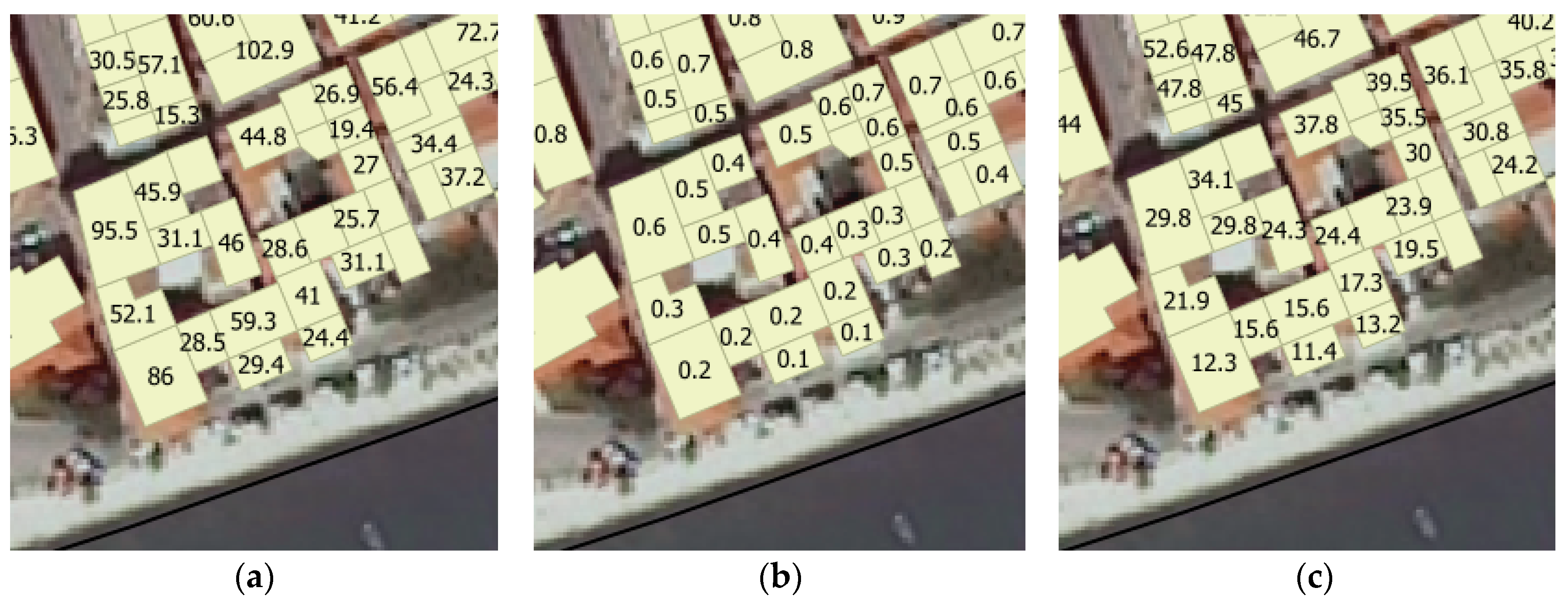
The building footprint areas were calculated from the polygons on an individual basis. Figure 2a shows the results. Elevation above the sea level was calculated as the mean value of the elevations covered by the building’s footprint. Figure 2b shows the results. Distance to coastline was calculated as the shortest distance from the building’s footprint to the coastline. Firstly, the polylines representing the buildings and coastline were converted to nodes, and for each building’s node, the distance to the coastline’s node was calculated. If necessary, the nodes representing the coastline could be densified. To obtain the shortest distance, the calculated distances from the nodes belonging to one building were grouped, and the minimal value was selected. Figure 2c shows the results of this process. Each step resulted in a new value being stored in the attribute tables of the Buildings.
2.4. Methods
Three methods are implemented:
- The Index method: crisp ranking by scores;
- The Index method: continuous ranking by functions;
- The Fuzzy logic method: ranking by membership functions.
To implement these methods, particularly to define the rankings, the contributions of the key geospatial parameters to vulnerability should be defined based on an expert evaluation of the study area.
For the City of Kaštela, the study presented in [44,45] defined the hazard zones for coastal flooding as a zone up to 1 m above sea level (already under flooding during storm surges): zone 2 is up to 2 m above sea level, and zone 3 is up to 3 m above sea level. For distance from the coastline, the contribution is defined as high for distances up to 35 m (which have daily and close visual contact with the sea), medium for distances from 35 to 75 m, and low for distances longer than 75 m. For the building’s footprint area, the contribution is defined based on the costs of building repair and insurance coverage [49]. The insurance coverage offered on the local market completely covers the building basement repair costs for approximately a 15 m2 footprint area, and the cost to repair an area of 45 m2 corresponds to the average annual wage per capita. Thus, a footprint area less than 15 m2 has a low contribution to vulnerability, that from 15–45 m2 has a medium contribution, and that larger than 45 m2 contributes highly to building vulnerability.
A further elaboration of the above defined contributions to vulnerability is not the focus of this research. Moreover, the definitions of the contributions are dependent on the specifics of the study area, and the analytical requirements cannot be generally defined. All three methods were implemented via the open source software QGIS and a spreadsheet calculator.
2.4.1. Index Method—Crisp Ranking by Scores
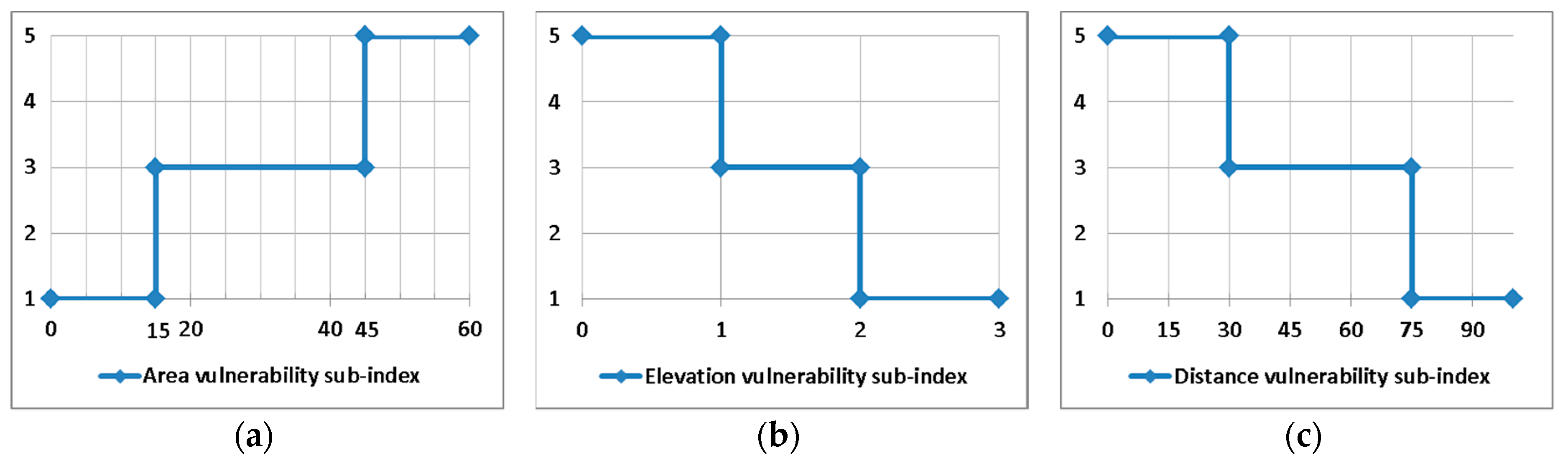
Using the contributions of the key geospatial parameters given by an expert’s evaluation, the vulnerability sub-indices are defined by the use of crisp values for ranking: 5 for high, 3 for medium, and 1 for low contributions (Table 1). The rankings are visualised in Figure 3. The attribute table of the Buildings was exported from QGIS [53], and further calculations were performed in a spreadsheet calculator using the expressions given in Table 1.
The definition of a single vulnerability for each building implies that the sub-indices should be integrated into one index called the single or final index. Various relevant approaches have been described and commented upon in the literature, and an overview is given in [1]. As this research was narrowed down to only the key geospatial parameters, and the intention was not to additionally quantify the contributions of vulnerability parameters, the simplest equation was used, featuring the average of the sub-indices (Equation (1)).
The calculated single indices are in the range of 1 to 5 and are further rounded to the nearest integers, 1, 2, 3, 4, and 5, representing the building vulnerability index and defining vulnerability using linguistic expressions as follows:
- 1—low vulnerability;
- 2—medium low vulnerability;
- 3—medium vulnerability;
- 4—medium high vulnerability;
- 5—high vulnerability.
2.4.2. Index Method—Continuous Ranking by Functions
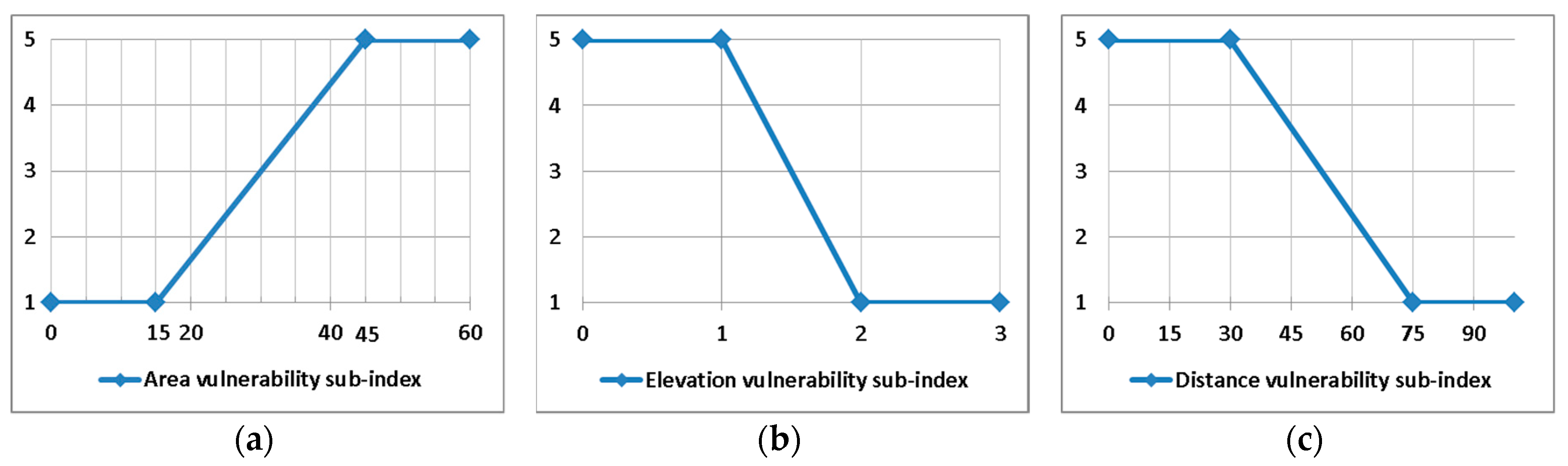
Here, the previously implemented Index method was modified such that instead of crisp rankings, continuous rankings were used. Using the contributions of key geospatial parameters to the building vulnerability, the vulnerability sub-indices were defined by using functions and assigning then the following values: 5 for a high contribution and 1 for a low contribution along with continuous values from 1,1 to 4,9 for a medium contribution (Table 2). The ranking functions are visualised in Figure 4. The calculations were done in a spreadsheet calculator using the expressions given in Table 2.
For a single vulnerability index of each building, the same definitions and calculations used for the Index method were employed, with the crisp rankings given in the previous paragraph (Section 2.4.1).
2.4.3. Fuzzy Logic Method—Ranking by Membership Functions
The Index method was modified such that instead of crisp rankings, fuzzy logic membership functions assigned a membership value to a fuzzy set. In fuzzy set theory, an element’s membership to a set is described by its membership function. The membership function values are between 0 and 1, indicating the degree of membership [48] and are described in a linguistic form such as “near” and “far”. Moreover, fuzzy logic offers the new concept of integrating the sub-indices into a single index via logical reasoning with a generalized modus ponens (rules of inference), as shown in Equation (2). In this research, a simplified fuzzy logic method is used. Here, the conclusion of a rule is not a fuzzy set but a number. The single index for each building is represented here with the final conclusion:
If Premise
(“Premise variable a” is “Fuzzy set A” and “Premise variable b” is “Fuzzy set B”…)
then Consequence
(“Consequence” is equal to “Number”).
(“Premise variable a” is “Fuzzy set A” and “Premise variable b” is “Fuzzy set B”…)
then Consequence
(“Consequence” is equal to “Number”).
To compute the final conclusion, the single index, several steps are implemented:
- Definition of rules based on fuzzy sets with a number for the conclusion (Equation (3));
- Calculation of the membership functions for the fuzzy sets (Equation (4));
- Calculation of the minimum membership function values per rule (Equation (5));
- Calculation of the conclusion value per rule (Equation (6));
- Computation of the final conclusion (Equation (7)).
Rule 1 with a consequence = C1 (number)
Rule 2 with a consequence = C2 (number)
…
Rule 2 with a consequence = C2 (number)
…
Membership function μA:X → [0,1] where μA(x) is the membership value of x in A
Min(Rule 1) = min (μA1(x), μB1(y), …)
Min(Rule 2) = min (μA2(x), μB2(y), …)
…
Min(Rule 2) = min (μA2(x), μB2(y), …)
…
Conclusion(Rule 1) = Min(Rule 1) · C1
Conclusion(Rule 2) = Min(Rule 2) · C2
…
Conclusion(Rule 2) = Min(Rule 2) · C2
…
Final conclusion = ∑ Conclusion(Rule i) / Σ Min(Rule i).
A brief description of the implemented steps follows. For each geospatial parameter, two fuzzy logic sets and their corresponding membership functions are defined, based on their contribution to building vulnerability, as defined in introduction of Section 2.4. Linear functions are used, because they were also employed in the previous method, so later methods could be compared. Table 3 provides their names and spreadsheet expressions for their calculations, while Figure 5 illustrates them.
To define the rules, all combinations of fuzzy sets representing geospatial parameters should be considered. Therefore, there are 8 rules listed in Table 4. These rules’ consequences (expressed as numbers and linguistic expressions) represent the vulnerability value that should be evaluated by an expert. The following steps include a calculation of the minimum membership function values per rule and a calculation of the conclusion value for the rule (a combination of Equations (5) and (6)); the spreadsheet expression is given in Table 4.
The final conclusion for each building is computed by Equation (7), and further rounded to the nearest integers of 1, 2, 3 4, and 5. Thus, the final conclusions represent the final building vulnerability indices expressed by linguistic expressions—the same ones used in the previous two methods.
3. Results
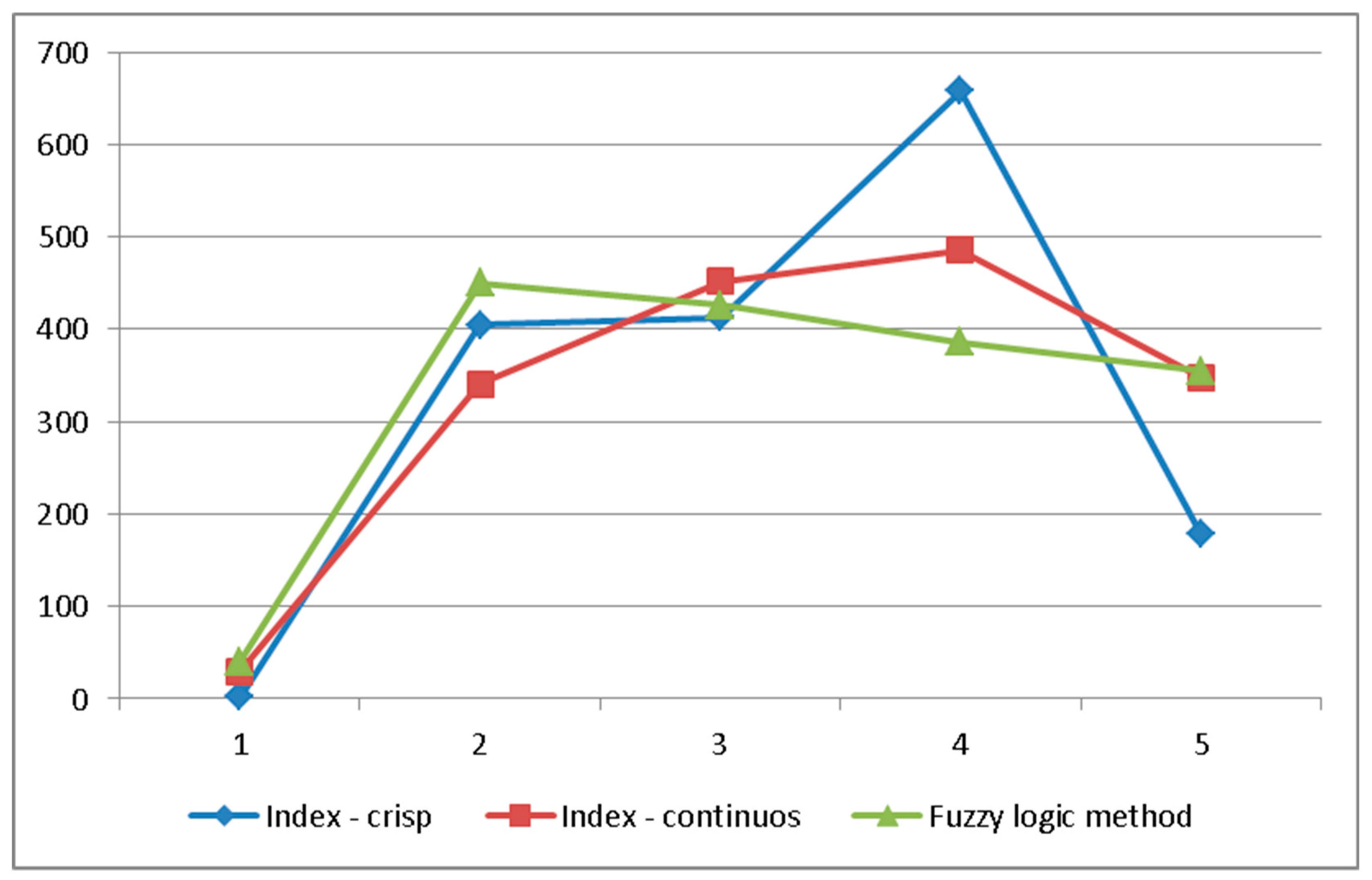
Using the same values for the contribution of key geospatial parameters but different methods for their rankings and integration resulted in significant differences in the vulnerability indices assigned to the buildings. The results are summarised in Table 5 and illustrated in Figure 6, Figure 7 and Figure 8.
The sums of single vulnerability indices for all the buildings calculated by the three methods do not show significant differences; the greatest difference is 4% of the sum value. When considering particular buildings, there is a significant difference in their assessment using these three methods.
Examining the graph given in Figure 6, the greatest differences are found for vulnerability index 4 (among all three methods), while for vulnerability index 5, the Index method with crisp rankings has a significantly lower number of buildings. By introducing continuous ranking for the Index method, the results are closer to the Fuzzy logic method results.
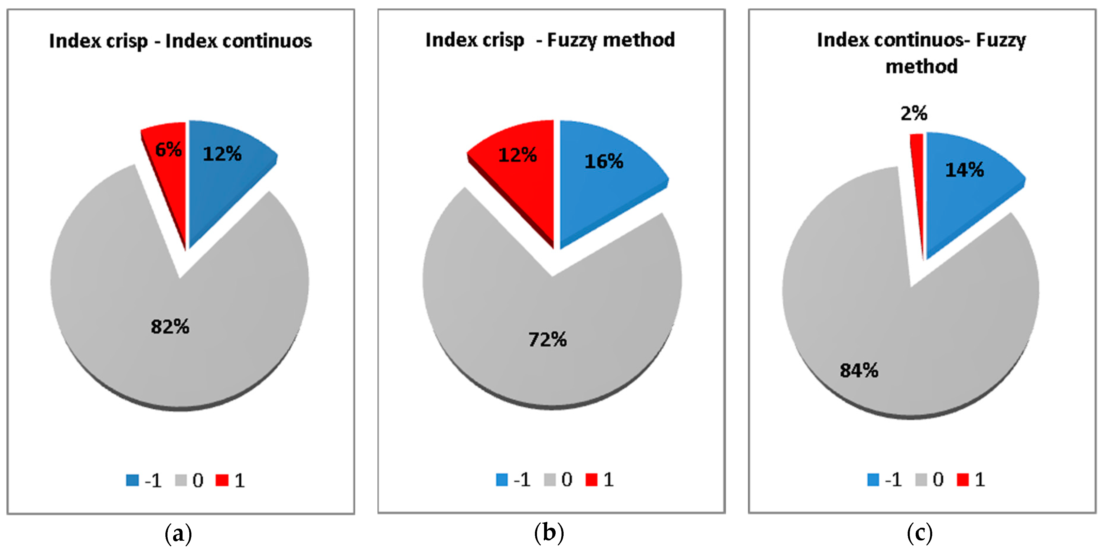
Examining the graphs given in Figure 7, the findings are as follows. Comparing the Index methods using crisp ranking with the methods using continuous ranking, there are significant differences in the building vulnerability assessment: 18% of buildings have a different vulnerability index, but there is no difference higher than 1 score. Comparing the Index method using crisp ranking and the Fuzzy logic method, the differences are even more significant: 28% of buildings have different vulnerability indexes, but, again, there is no difference higher than 1 score. Finally, comparing the Index method using continuous ranking and the Fuzzy logic method, there are still significant differences; however, these differences are a bit smaller: 16% of buildings have a different vulnerability index.
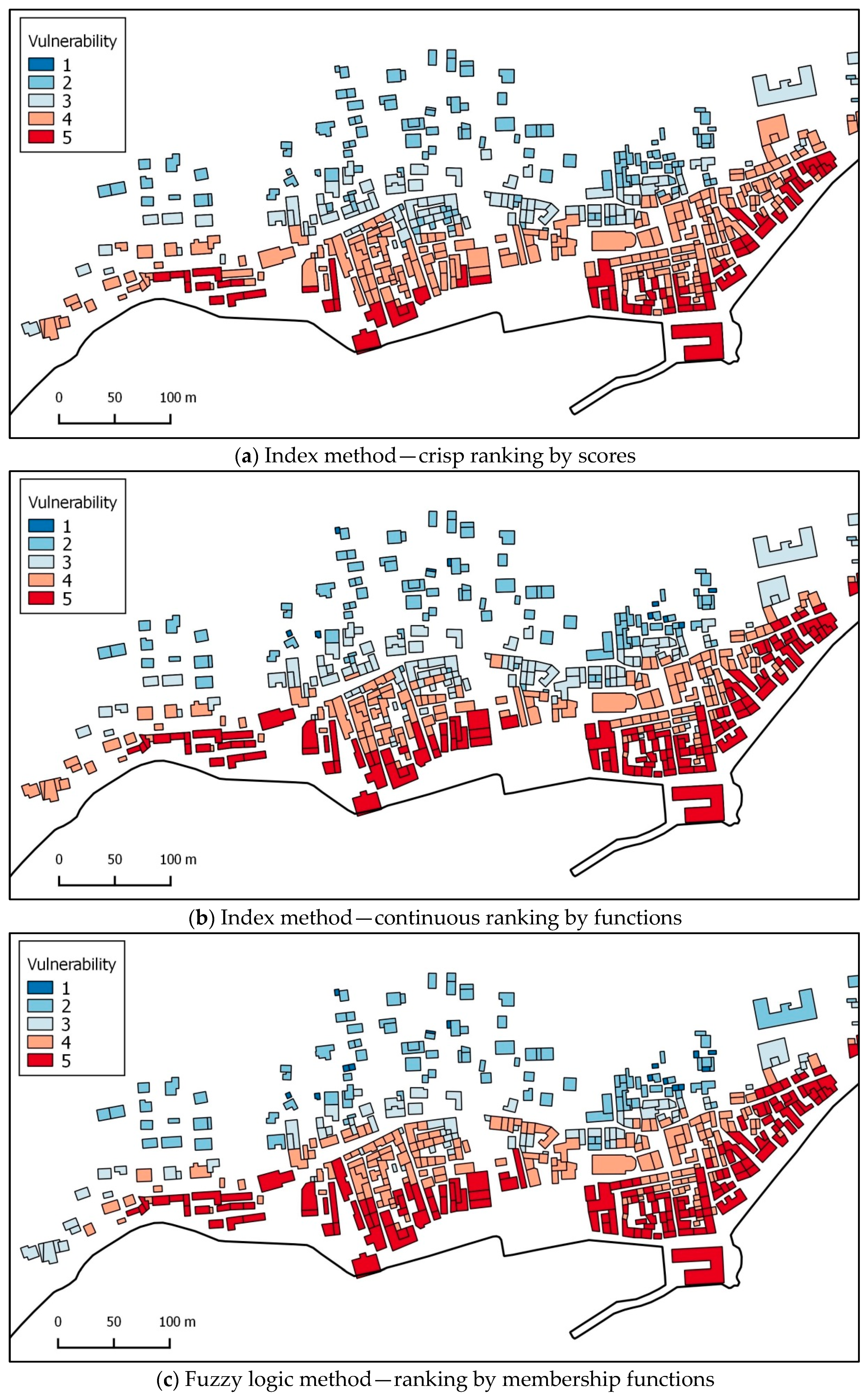
Finally, the spreadsheet table with all the calculated values is joined with the layer Building in QGIS, and the visualisations are performed. Figure 8 presents maps showing the single vulnerability indices for buildings calculated by the three methods: (a) the Index method—crisp ranking by scores; (b) the Index method—continuous ranking by functions; (c) and the Fuzzy logic method—ranking by membership functions. The highest vulnerability value (5) is coloured with red, and the colours change gradually to blue, which represents the lowest vulnerability value of 1. Summarising all the previous comparisons and observing the visualisations in Figure 8, one can conclude that the Index method with crisp ranking assigns more medium values (2, 3, and 4) and many fewer extreme values (1 and 5). The other two methods assigned significantly more buildings to the highest value of 5 (approximately 10% more), with more buildings assuming the lowest value because, in the Index method with crisp ranking, there are almost no values of 1.
4. Discussion
The above results show that there are significant differences in the vulnerability indices assigned to the buildings calculated by the various methods. Hence, the question arises: which method should one choose for a vulnerability assessment?
For the appropriate spatial units to be used, the relevant works clearly show that buildings are adequate units, as they are the key assets exposed. Moreover, socio–economic parameters are assigned to households, and can thus be easily assigned to building footprints. All three methods can use buildings or any other exposed assets as spatial units for vulnerability assessment.
Uncertainties in a vulnerability assessment sometimes originate in the data. Vagueness in the attribute values describing features cannot be avoided and causes uncertainties in the feature descriptions. The proposed Fuzzy logic method using the membership functions could model these uncertainties, while the other two methods cannot. Vagueness in the definition of boundaries causes uncertainties in the position and geometries of features. The solution proposed by the relevant work is based on Fuzzy Spatial Data Types whose implementation is complex and thus is not included in any of the proposed methods. Therefore, these types of uncertainties remain. There is also an uncertainty in the assessment caused by the aggregation of the key parameter values for each building. For example, the mean elevation and the shortest distance are calculated and assigned to each building, including their values within the building’s footprint. Another source of uncertainty lies in the expert evaluation of the key parameters’ contributions to vulnerability. These two uncertainties can be modelled by the membership functions; thus, the Fuzzy logic method can solve these uncertainties, while other the two methods cannot.
Crisp classifications, when applied to continuous phenomena, are unsatisfying. Both newly proposed methods overcome the pitfalls of existing Index-based methods, either by the introduction of functions or of fuzzy membership functions.
Finally, the methods are evaluated by how easily they can be applied by the local administration and accepted by all the participants. All three methods use widely available and open tools, as well as commonly available data for local administration. The Fuzzy logic method requires participant efforts in understanding the concepts of fuzzy set theory and fuzzy logic, while the other two methods are much simpler and more straightforward. However, the Fuzzy logic method is superior in supporting qualitative approaches and provides semantic values common to human perception. This is achieved by turning the quantitative parameters into linguistic variables such as “low” or “high” and by expressing the rules with linguistic expressions.
5. Conclusions
At the beginning of this research, we posed four questions that address the requirements of using an Index-based method for a household level analysis. Table 6 summarises a comparison of the existing method and the two newly proposed methods based on how they answer these questions.
Table 6 clearly shows that the Fuzzy logic method satisfies almost all the requirements and significantly improves the existing Index-based method, but it requires more effort from the human side. The local administration’s staff and urban planners should become familiar with fuzzy set and fuzzy logic concepts, or they could become an obstacle to the method’s application.
The Index method with continuous ranking introduces only one improvement: the modelling of continuous phenomena by functions. However, the results are significantly different from those obtained by the existing Index method with crisp ranking, and are instead closer to those of the Fuzzy logic method. The advantage of this method over the Fuzzy logic method is that the Index method is more simply understood by non-experts, and thus has more potential to be accepted and implemented by local administrations.
To determine which method to choose, there is always a trade-off between the comprehensiveness of the method and the resources needed for its implementation. This research showed that Index method with continuous ranking could be used as an alternative to the Fuzzy logic method. Thus, the Index method with continuous ranking is proposed for use by local administration as a simple and viable method that still improves vulnerability assessment at the household level.
Funding
This research was partially supported through the project KK.01.1.1.02.0027, a project co-financed by the Croatian Government and the European Union through the European Regional Development Fund–the Competitiveness and Cohesion Operational Programme.
Acknowledgments
The author is grateful to the editors and reviewers for their valuable comments on the manuscript.
Conflicts of Interest
The author declares no conflict of interest.
References
- Ramieri, E.; Hartley, A.; Barbanti, A.; Santos, F.D.; Gomes, A.; Hilden, M.; Laihonen, P.; Marinova, N.; Santini, M. Methods for Assessing Coastal Vulnerability to Climate Change; Technical Paper 1; European Topic Centre on Climate Change Impacts, Vulnerability and Adaptation: Bologna, Italy, 2011. [Google Scholar]
- Lavell, A.; Oppenheimer, M.; Diop, C.; Hess, J.; Lempert, R.; Li, J.; Muir-Wood, R.; Myeong, S. Climate change: New dimensions in disaster risk, exposure, vulnerability, and resilience. In Managing the Risks of Extreme Events and Disasters to Advance Climate Change Adaptation; A Special Report of Working Groups I and II of the Intergovernmental Panel on Climate Change, (IPCC); Field, C.B., Barros, V., Stocker, T.F., Qin, D., Dokken, D.J., Ebi, K.L., Mastrandrea, M.D., Mach, K.J., Plattner, G.-K., Allen, S.K., et al., Eds.; Cambridge University Press: Cambridge, UK; New York, NY, USA, 2012; pp. 25–64. [Google Scholar]
- Koerth, J.; Vafeidis, A.; Hinkel, J. Household-Level Coastal Adaptation and Its Drivers: A Systematic Case Study Review. Risk Anal. 2016, 37, 629–646. [Google Scholar] [CrossRef] [PubMed]
- Moret, W. Vulnerability Assessment Methodologies: A Review of the Literature; Family Health International (FHI 360): Durham, NC, USA, 2014. [Google Scholar]
- Brooks, N. Vulnerability, Risk and Adaptation: A Conceptual Framework; Working Paper No. 38; Tyndall Centre for Climate Change Research: Norwich, UK, 2003. [Google Scholar]
- Jean-Baptiste, N.; Kuhlicke, C.; Kunath, A.; Kabisch, S. Review and Evaluation of Existing Vulnerability Indicators for Assessing Climate Related Vulnerability in Africa; No. 07; UFZ-Bericht, Helmholtz-Zentrum für Umweltforschung: Leipzig, Germany, 2011. [Google Scholar]
- Almås, A.J.; Hygen, H. Impacts of sea level rise towards 2100 on buildings in Norway. Build. Res. Inf. 2012, 40, 245–259. [Google Scholar] [CrossRef]
- Gornitz, V.M. Vulnerability of the East coast, U.S.A. to future sea level rise. J. Coast. Res. 1990, 9, 201–237. [Google Scholar]
- Gornitz, V.M. Global coastal hazards from future sea level rise. Palaeogeogr, Palaeoclimatol. Palaeoecol. (Glob. Planet. Chang. Sect.) 1991, 89, 379–398. [Google Scholar] [CrossRef]
- Ozyurt, G. Vulnerability of Coastal Areas to Sea Level Rise: A Case of Study on Göksu Delta. Master’s Thesis, Middle-East Technical University, Ankara, Turkey, January 2007. Available online: http://etd.lib.metu.edu.tr/upload/12608146/index.pdf (accessed on 8 October 2011).
- Szlafsztein, C.; Sterr, H. A GIS-based vulnerability assessment of coastal natural hazards, State of Para, Brazil. J. Coast. Conserv. 2007, 11, 53–66. [Google Scholar] [CrossRef]
- McLaughlin, S.; Cooper, J.A.G. A multi-scale coastal vulnerability index: A tool for coastal managers? Environ. Hazards 2010, 9, 233–248. [Google Scholar] [CrossRef]
- Deduce Consortium. Available online: https://www.msp-platform.eu/practices/assessment-model- sustainable -development-european-coastal-zones (accessed on 15 January 2020).
- Torresan, S.; Zabeo, A.; Rizzi, J.; Critto, A.; Pizzol, L.; Giove, S.; Marcomini, A. Risk assessment and decision support tools for the integrated evaluation of climate change on coastal zones. In Proceedings of the International Congress on Environmental Modelling and Software Modelling for Environment’s Sake, Fifth Biennial Meeting, Ottawa, ON, Canada, 5–8 July 2010; Swayne, D.A., Wanhong, Y., Voinov, A.A., Rizzoli, A., Filatova, T., Eds.; International Environmental Modelling and Software Society: Manno, Switzerland, 2010. [Google Scholar]
- Risk Assessment of Coastal Erosion: Part One. Available online: http://randd.defra.gov.uk/Document.aspx?Document=FD2324_7453_TRP.pdf (accessed on 15 January 2020).
- DIVA. Available online: https://www.pik-potsdam.de/research/projects/projects-archive/favaia/diva (accessed on 15 January 2020).
- Delft3D Modelling Suite. Available online: https://www.deltares.nl/en/software/delft3d-4-suite/ (accessed on 15 January 2020).
- Miller, A.; Reiter, J.; Weiland, U. Assessment of urban vulnerability towards floods using an indicator-based approach—A case study for Santiago de Chile. Nat. Hazards Earth Syst. Sci. 2011, 11, 2107–2123. [Google Scholar] [CrossRef] [Green Version]
- Kantamaneni, K.; Du, X.; Aher, S.; Singh, R. Building Blocks: A Quantitative Approach for Evaluating Coastal Vulnerability. Water 2017, 9, 905. [Google Scholar] [CrossRef] [Green Version]
- Kim, Y.; Chung, E.S. An index-based robust decision making framework for watershed management in a changing climate. Sci. Total. Environ. 2014, 473–474, 88–102. [Google Scholar] [CrossRef]
- Koroglu, A.; Ranasinghe, R.; Jiménez, J.; Dastgheib, A. Comparison of Coastal Vulnerability Index applications for Barcelona Province. Ocean Coast. Manag. 2019, 178, 104799. [Google Scholar] [CrossRef]
- Basofi, A.; Fariza, A.; Dzulkarnain, M.R. Landslides susceptibility mapping using fuzzy logic: A case study in Ponorogo, East Java, Indonesia. In Proceedings of the 2016 International Conference on Data and Software Engineering (ICoDSE), Denpasar, Indonesia, 26–27 October 2016; pp. 1–7. [Google Scholar] [CrossRef]
- Wardhana, M.; Sofwan, A.; Setiawan, I. Fuzzy Logic Method Design for Landslide Vulnerability. E3S Web Conf. 2019, 125, 03004. [Google Scholar] [CrossRef]
- Sadrykia, M.; Delavar, M.; Mehdi, Z.A. GIS-Based Fuzzy Decision Making Model for Seismic Vulnerability Assessment in Areas with Incomplete Data. ISPRS Int. J. Geo-Inf. 2017, 6, 119. [Google Scholar] [CrossRef] [Green Version]
- Jadidi, M.; Mostafavi, M.A.; Bédard, Y.; Kyarash, S. Spatial Representation of Coastal Risk: A Fuzzy Approach to Deal with Uncertainty. ISPRS Int. J. Geo-Inf. 2014, 3, 1077–1100. [Google Scholar] [CrossRef]
- Rashetnia, S. Flood Vulnerability Assessment by Applying a Fuzzy Logic Method: A Case Study from Melbourne. Master’s Thesis, Victoria University, Melbourne, Australia, August 2016. [Google Scholar]
- Galindo, J.; Schneider, M. Fuzzy Spatial Data Types for Spatial Uncertainty Management in Databases. In Handbook of Research on Fuzzy Information Processing in Databases, 1st ed.; Galindo, J., Ed.; IGI Global: Hershey, PA, USA, 2008; pp. 154–196. [Google Scholar] [CrossRef]
- Chu, T.C. Selecting plant location via a Fuzzy TOPSIS approach. Int. J. Adv. Manuf. Technol. 2002, 20, 859–864. [Google Scholar] [CrossRef]
- Yong, D. Plant location selection based on fuzzy TOPSIS. Int. J. Adv. Manuf. Technol. 2006, 28, 839–844. [Google Scholar] [CrossRef]
- Jun, K.S.; Chung, E.S.; Kim, Y.G.; Kim, Y. A fuzzy multicriteria decision approach to flood risk vulnerability in South Korea by considering climate change impacts. Expert Syst. Appl. 2013, 40, 1003–1013. [Google Scholar] [CrossRef]
- Kim, Y.; Chung, E.S.; Jun, S.M.; Kim, S.U. Prioritizing the best sites for treated wastewater use in an urban watershed using Fuzzy TOPSIS. Resour. Conserv. Recycl. 2013, 73, 23–32. [Google Scholar] [CrossRef]
- Jara, J.; Acevedo-Crespo, R. Crisp Classifiers vs. Fuzzy Classifiers: A Statistical Study. Comput. Vision 2009, 5495, 440–447. [Google Scholar] [CrossRef]
- Vadiati, M.; Asghar, M.A.; Nakhaei, M.; Adamowski, J.; Akbarzadeh, A.H. A fuzzy-logic based decision-making approach for identification of groundwater quality based on groundwater quality indices. J. Environ. Manag. 2016, 184. [Google Scholar] [CrossRef]
- Valentini, E.; Nguyen Xuan, A.; Filipponi, F.; Taramelli, A. Coastal vulnerability assessment using Fuzzy Logic and Bayesian Belief Network approaches. In Geophysical Research Abstracts 201, 19, EGU2017-18063; European Geosciences Union General Assembly: Vienna, Austria, 2017. [Google Scholar]
- Akter, T.; Simonovic, S. Aggregation of Fuzzy Views of a Large Number of Stakeholders for Multi-Objective Flood Management Decision-Making. J. Environ. Manag. 2005, 7, 133–143. [Google Scholar] [CrossRef]
- Lee, G.; Jun, K.S.; Eun-Sung, C. Group decision-making approach for flood vulnerability identification using the fuzzy VIKOR method. Nat. Hazards Earth Syst. Sci. Discuss. 2014, 2. [Google Scholar] [CrossRef] [Green Version]
- Shan, X.; Wen, J.; Zhang, M.; Wang, L.; Ke, Q.; Li, W.; Du, S.; Shi, Y.; Chen, K.; Liao, B.; et al. Scenario-Based Extreme Flood Risk of Residential Buildings and Household Properties in Shanghai. Sustainability 2019, 11, 3202. [Google Scholar] [CrossRef] [Green Version]
- Jadidi, M.; Mostafavi, M.A.; Bédard, Y.; Long, B.; Grenier, E. Using geospatial business intelligence paradigm to design a multidimensional conceptual model for efficient coastal erosion risk assessment. J. Coast. Conserv. 2013, 17, 527–543. [Google Scholar] [CrossRef]
- Bermúdez, M.; Zischg, A.P. Sensitivity of flood loss estimates to building representation and flow depth attribution methods in micro-scale flood modelling. Nat. Hazards 2018, 92, 1633–1648. [Google Scholar] [CrossRef] [Green Version]
- Hatzikyriakou, A.; Lin, N. Assessing the Vulnerability of Structures and Residential Communities to Storm Surge: An Analysis of Flood Impact during Hurricane Sandy. Front. Built Environ. 2018, 4. [Google Scholar] [CrossRef]
- Swart, R.; Fons, J.; Geertsema, W.; Hove, L.V.; Jacobs, C. Urban Vulnerability Indicators. A Joint Report of ETC-CCA and ETC-SIA. ETC CCA/ETC/SIA; Technical Report 01; ETC CCA: Bologna, Italy, 2012. [Google Scholar]
- Coastal Plan for the Šibenik-Knin County (2015, PAP/RAC). Available online: http://iczmplatform. org//storage/documents/pEoju2FqfXjzPoYBLsKZiD3o6ONBXxJ44RTWFt7P.pdf (accessed on 15 January 2020).
- Andričević, R.; Knezić, S.; Vranješ, M.; Baučić, M.; Jajac, N. Report on Initial Flood Vulnerability Assessment in the Sava River Basin, Pilot Project on Climate Change: Building the Link between Flood Risk Management Planning and Climate Change Assessment in the Sava River Basin, the International Sava River Basin Commission, 2013. Available online: https://www.savacommission.org/project_detail/17/1 (accessed on 15 January 2020).
- Margeta, J.; Vilibić, I.; Jakl, Z.; Marasović, K.; Petrić, L.; Mandić, A.; Grgić, A.; Bartulović, H.; Baučić, M. Draft version: Coastal Action Plan for the City of Kaštela; Technical Report; JU RERA: Split, Croatia, 2019. [Google Scholar]
- Baučić, M.; Ivić, M.; Jovanović, N.; Bačić, S. Vulnerability analysis for the integrated coastal zone management plan of the City of Kaštela in Croatia. ISPRS–Int. Arch. Photogramm. Remote Sens. Spat. Inf. Sci. 2019, XLII-3/W8, 59–63. [Google Scholar] [CrossRef] [Green Version]
- Begg, S.H.; Welsh, M.B.; Bratvold, R.B. Uncertainty vs. Variability: What’s the Difference and Why is it Important? In Proceedings of the Society of Petroleum Engineers Hydrocarbon Economics and Evaluation Symposium, Houston, TX, USA, 19–20 May 2014. [Google Scholar] [CrossRef] [Green Version]
- Fisher, P.; Comber, A.; Wadsworth, R. Approaches to Uncertainty in Spatial Data. In Fundamentals of Spatial Data Quality, 1st ed.; Devillers, R., Jeansoulin, R., Eds.; ISTE Ltd.: London, UK, 2010; pp. 43–59. [Google Scholar] [CrossRef]
- Zadeh, L.A. Fuzzy sets. Inf. Control 1965, 8, 338–353. [Google Scholar] [CrossRef] [Green Version]
- Proverbs, D.G.; Soetanto, R. Flood Damaged Property, A Guide to Repair, 1st ed.; Blackwell Publishing Ltd: Hoboken, NJ, USA, 2004. [Google Scholar]
- Open Digital Elevation Model (OpenDEM). Available online: https://www.opendem.info/index.html (accessed on 15 January 2020).
- Šimek, K.; Medak, D.; Medved, I. Analiza visinske točnosti službenoga vektorskoga digitalnoga modela reljefa Republike Hrvatske dobivenog fotogrametrijskom restitucijom. Geod. List 2018, 3, 217–230. [Google Scholar]
- Brovelli, M.; Zamboni, G.A. New Method for the Assessment of Spatial Accuracy and Completeness of OpenStreetMap Building Footprints. ISPRS Int. J. Geo-Inf. 2018, 7, 289. [Google Scholar] [CrossRef] [Green Version]
- QGIS. A Free and Open Source Geographic Information System. Available online: https://qgis.org/en/site/ (accessed on 15 January 2020).
Figure 1.
Research steps.

Figure 2.
Maps showing the key geospatial parameters for each building in the study area: (a) the building’s footprint area (m2); (b) the elevation above sea level (m); (c) the distance to coastline (m).
Figure 2.
Maps showing the key geospatial parameters for each building in the study area: (a) the building’s footprint area (m2); (b) the elevation above sea level (m); (c) the distance to coastline (m).

Figure 3.
Graphs showing the crisp rankings of the key geospatial parameters—vulnerability sub-indices: (a) for the building’s footprint area; (b) for elevation above the sea level; and (c) for distance to coastline.
Figure 3.
Graphs showing the crisp rankings of the key geospatial parameters—vulnerability sub-indices: (a) for the building’s footprint area; (b) for elevation above the sea level; and (c) for distance to coastline.

Figure 4.
Graphs showing the continuous rankings of the key geospatial parameters—vulnerability sub-indices: (a) for the building’s footprint area; (b) for the elevation above sea level; (c) for the distance to coastline.
Figure 4.
Graphs showing the continuous rankings of the key geospatial parameters—vulnerability sub-indices: (a) for the building’s footprint area; (b) for the elevation above sea level; (c) for the distance to coastline.

Figure 5.
Graphs showing the fuzzy membership functions of key geospatial parameters: (a) small and large buildings for the building’s footprint area; (b) low and high elevations for elevation above the sea level; (c) near and far from the sea for distance to coastline.
Figure 5.
Graphs showing the fuzzy membership functions of key geospatial parameters: (a) small and large buildings for the building’s footprint area; (b) low and high elevations for elevation above the sea level; (c) near and far from the sea for distance to coastline.

Figure 6.
Graph showing the number of buildings with assigned single vulnerability indices of 1, 2, 3, 4, or 5, calculated by the three methods.
Figure 6.
Graph showing the number of buildings with assigned single vulnerability indices of 1, 2, 3, 4, or 5, calculated by the three methods.

Figure 7.
Graphs showing how many buildings have differences in their single vulnerability indexes calculated by the two methods (a blue colour represents a −1 score, red is a 1 score, and grey means no difference): (a) Index method with crisp ranking—Index method with continuous ranking; (b) Index method with crisp ranking—Fuzzy logic method; and (c) the Index method with continuous ranking— Fuzzy logic method.

Figure 8.
Maps showing the single vulnerability index for each building in the study area (an excerpt) calculated by the methods: (a) the Index method—crisp ranking by scores; (b) the Index method—continuous ranking by functions; and (c) the Fuzzy logic method—ranking by membership functions.
Figure 8.
Maps showing the single vulnerability index for each building in the study area (an excerpt) calculated by the methods: (a) the Index method—crisp ranking by scores; (b) the Index method—continuous ranking by functions; and (c) the Fuzzy logic method—ranking by membership functions.


Table 1.
Crisp ranking by scores: the vulnerability sub-indices Varea, Velevation, and Vdistance.
| Geospatial Parameter | Vulnerability Sub-Index 5 (High) | Vulnerability Sub-Index 3 (Medium) | Vulnerability Sub-Index 1 (Low) | Spreadsheet Expression for Calculation |
|---|---|---|---|---|
| building’s footprint area | >45 m2 | 15–45 m2 | <15 m2 | =IF(“area”<=15;1;IF(“area”<45;3;5)) |
| elevation above sea level | <1m | 1–2 m | >2 m | =IF(“elevation”<=1;5;IF(“elevation”<2;3;1)) |
| distance to the coastline | <30 m | 30–75 m | >75 m | =IF(“distance”<=30;5;IF(“distance”<75;3;1)) |
Table 2.
Continuous rankings: the vulnerability sub-indices Varea, Velevation, and Vdistance.
| Geospatial Parameter | Vulnerability Sub-Index 5 (High) | Vulnerability Sub-Index 4,9–1,1 (Medium) | Vulnerability Sub-Index 1 (Low) | Spreadsheet Expression for Calculation |
|---|---|---|---|---|
| building’s footprint area | >45 m2 | 15–45 m2 | <15 m2 | =IF(“area”<=15;1;IF(“area”<45;(4/30*(“area”-15)+1);5)) |
| elevation above the sea level | <1m | 1–2 m | >2 m | =IF(“elevation”<=1;5;IF((“elevation”<2;(-4*(“elevation”+9);1)) |
| distance to the coastline | <30 m | 30–75 m | >75 m | =IF(“distance”<=30;5;IF(“distance”<75;(-4/45*(“distance”-30)+5);1)) |
Table 3.
Fuzzy sets and membership functions for the key geospatial parameters.
| Geospatial Parameter | Linguistic Variable - Fuzzy Set - | Spreadsheet Expression for the Calculation of Fuzzy Membership Function Values |
|---|---|---|
| building’s footprint area | Small building (SB) | =IF(“area”<=15;1;IF(“area”<45;(45-“area”)/30;0)) |
| Large building (LB) | =IF(“area”<=15;0;IF(“area”<45;(“area”-15)/30;1)) | |
| elevation above sea level | Low elevation (LE) | =IF(“elevation”<=1;1;IF(“elevation”<2;(2-“elevation”);0)) |
| High elevation (HE) | =IF(“elevation”<=1;0;IF(“elevation”<2;(“elevation”-1);1)) | |
| distance to coastline | Near to the sea (NS) | =IF(“distance”<=30;1;IF(“distance”<75;(75-“distance”)/45;0)) |
| Far from the sea (FS) | =IF(“distance”<=30;0;IF(“distance”<75;(“distance”-30)/45;1)) |
Table 4.
Rules with their linguistic expressions and spreadsheet expressions for the calculation of the rule conclusions.
Table 4.
Rules with their linguistic expressions and spreadsheet expressions for the calculation of the rule conclusions.
| No | Rule Premise | Consequence as a Fuzzy Singleton (Vulnerability Value) | Linguistic Expression of the Vulnerability Value | Rule Conclusion (Spreadsheet Expression) |
|---|---|---|---|---|
| 1 | If The building is small (SB), its elevation is low (LE), and it is near the sea (NS) | 4 | Medium high vulnerability | =MIN(SB;LE;NS)*4 |
| 2 | If The building is small (SB), its elevation is low (LE), and it is far from the sea (FS) | 3 | Medium vulnerability | =MIN(SB;LE;FS)*3 |
| 3 | If The building is small (SB), its elevation is high (HE), and it is near the sea (NS) | 2 | Medium low vulnerability | =MIN(SB;HE;NS)*2 |
| 4 | If The building is small (SB), its elevation is high (HE), and it is far from the sea (FS) | 1 | Low vulnerability | =MIN(SB;HE;FS)*1 |
| 5 | If The building is large (LB), its elevation is low (LE), and it is near the sea (NS) | 5 | High vulnerability | =MIN(LB;LE;NS)*5 |
| 6 | If The building is large (LB), its elevation is low (LE), and it is far from the sea (FS) | 4 | Medium high vulnerability | =MIN(LB;LE;FS)*4 |
| 7 | If The building is large (LB) its elevation is high (HE), and it is near the sea (NS) | 3 | Medium vulnerability | =MIN(LB;HE;NS)*3 |
| 8 | If The building is large (LB), its elevation is high (HE), and it is far from the sea (FS) | 2 | Medium low vulnerability | =MIN(LB;HE;FS)*2 |
Table 5.
Numbers of buildings with vulnerability index 1, 2, 3, 4, and 5, calculated by the three methods.
Table 5.
Numbers of buildings with vulnerability index 1, 2, 3, 4, and 5, calculated by the three methods.
| Single Vulnerability Index | Index Method—Crisp Ranking | Index Method—Continuous Ranking | Fuzzy Logic Method |
|---|---|---|---|
| 1 | 2 | 30 | 40 |
| 2 | 405 | 341 | 450 |
| 3 | 413 | 452 | 426 |
| 4 | 658 | 486 | 386 |
| 5 | 179 | 348 | 355 |
| Total number of buildings | 1657 | 1657 | 1657 |
| Sum of single vulnerability indices for all buildings | 5578 | 5752 | 5537 |
Table 6.
A comparison of the methods satisfying the requirements for the household level analysis.
| Question | Requirements of the Method for the Household Level Analysis | Index Method—Crisp Ranking | Index Method—Continuous Ranking | Fuzzy Logic Method |
|---|---|---|---|---|
| Assets exposed, e.g., buildings | yes | yes | yes |
| Description uncertainties | no | no | yes |
| Boundary uncertainties | no | no | no | |
| Key parameter value uncertainties | no | no | yes | |
| Expert evaluation uncertainties | no | no | yes | |
| Modelling continuous phenomena | no | yes | yes |
| Method easily understood | yes | yes | no |
| Using available tools and data | yes | yes | yes | |
| Supports qualitative approach | no | no | yes | |
| Semantics common to human perception | no | no | yes |
© 2020 by the author. Licensee MDPI, Basel, Switzerland. This article is an open access article distributed under the terms and conditions of the Creative Commons Attribution (CC BY) license (http://creativecommons.org/licenses/by/4.0/).
Share and Cite
MDPI and ACS Style
Baučić, M. Household Level Vulnerability Analysis—Index and Fuzzy Based Methods. ISPRS Int. J. Geo-Inf. 2020, 9, 263. https://0-doi-org.brum.beds.ac.uk/10.3390/ijgi9040263
AMA Style
Baučić M. Household Level Vulnerability Analysis—Index and Fuzzy Based Methods. ISPRS International Journal of Geo-Information. 2020; 9(4):263. https://0-doi-org.brum.beds.ac.uk/10.3390/ijgi9040263
Chicago/Turabian StyleBaučić, Martina. 2020. "Household Level Vulnerability Analysis—Index and Fuzzy Based Methods" ISPRS International Journal of Geo-Information 9, no. 4: 263. https://0-doi-org.brum.beds.ac.uk/10.3390/ijgi9040263
Note that from the first issue of 2016, this journal uses article numbers instead of page numbers. See further details here.