Representing Complex Evolving Spatial Networks: Geographic Network Automata


Spatial Analysis and Modeling Lab, Department of Geography, Simon Fraser University, Burnaby, BC V5A 1S6, Canada
*
Author to whom correspondence should be addressed.
ISPRS Int. J. Geo-Inf. 2020, 9(4), 270; https://0-doi-org.brum.beds.ac.uk/10.3390/ijgi9040270
Submission received: 24 February 2020
/
Revised: 9 April 2020
/
Accepted: 16 April 2020
/
Published: 20 April 2020
Abstract
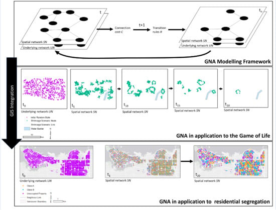
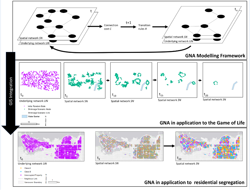
:Many real-world spatial systems can be conceptualized as networks. In these conceptualizations, nodes and links represent system components and their interactions, respectively. Traditional network analysis applies graph theory measures to static network datasets. However, recent interest lies in the representation and analysis of evolving networks. Existing network automata approaches simulate evolving network structures, but do not consider the representation of evolving networks embedded in geographic space nor integrating actual geospatial data. Therefore, the objective of this study is to integrate network automata with geographic information systems (GIS) to develop a novel modelling framework, Geographic Network Automata (GNA), for representing and analyzing complex dynamic spatial systems as evolving geospatial networks. The GNA framework is implemented and presented for two case studies including a spatial network representation of (1) Conway’s Game of Life model and (2) Schelling’s model of segregation. The simulated evolving spatial network structures are measured using graph theory. Obtained results demonstrate that the integration of concepts from geographic information science, complex systems, and network theory offers new means to represent and analyze complex spatial systems. The presented GNA modelling framework is both general and flexible, useful for modelling a variety of real geospatial phenomena and characterizing and exploring network structure, dynamics, and evolution of real spatial systems. The proposed GNA modelling framework fits within the larger framework of geographic automata systems (GAS) alongside cellular automata and agent-based modelling.
1. Introduction
As geospatial data becomes increasingly available, networks are used as a powerful conceptual framework to represent and analyze a wide array of complex spatial systems in social, urban, and ecological contexts [1,2,3]. The conceptualization of complex spatial systems as networks begins from the bottom-up, where system components are represented as georeferenced nodes and interactions between components are represented as links. Sets of local interactions between nodes form the global network structure. The representation of complex spatial systems as networks offers a well-developed toolkit for analysis [4,5]. Specifically, graph theory can be applied to describe the spatial structures of real phenomena and explore the tightly coupled relationship between spatial structure and spatial dynamics.
Network dynamics can be distinguished between dynamics on a network or the dynamics of networks [6]. In the former, the information or materials dynamically propagate through a set of spatially arranged nodes and links. For example, in ecology, the spatio-temporal dynamics of species dispersal is highly dependent on the spatial structure of habitat features across the landscape [3]. Likewise, in epidemiology, the spatio-temporal dynamics of disease spread is forecasted using the spatial structure of human contact networks [7]. In an urban context, a variety of transportation networks determine dynamics of human mobility [8]. The latter, dynamics of networks refers to dynamic changes in the network structure also known as network evolution. In this process, nodes and links are added, removed, rewired, or change properties over space and time [9]. Network evolution occurs as a function of the dynamics of the network itself, interactions between the network and the surrounding matrix, and the dynamics tightly-coupled to the network structure [10]. For example, dynamics of species dispersal may, in turn, affect the connectivity of the landscape, dynamics of disease spread may alter the human contact network, and traffic may damage streets, forcing their closure or require the construction of new streets to reduce congestion, thus forcing the evolution of transportation networks.
Network evolution is not well understood since detailed datasets representing real phenomena as networks over geographic space and time have been limited due to the lack of appropriate datasets. Conventional spatial network analysis tends to focus on describing and cataloguing static spatial network structures or exploring the effect of static spatial network structures on spatial dynamics. Some examples of this include exploring processes of gentrification on a static network of residential properties [11], ecological dispersal dynamics on static landscape connectivity networks [3,12], mobility dynamics on static road networks [13,14], and epidemics on static contact networks [7,15] and on airline networks [16].
Models representing phenomena such as predator–prey dynamics [17], fungal growth [9], and human epidemics [18] as evolving non-spatial networks have been developed by applying sub-rules representing network dynamics to network structures that alter the network structure itself over time. This methodology was formalized as network automata (NA) [9,19] where network topology changes over time. However, these proposed NA frameworks are not integrated with geographic information systems (GIS) nor do they use actual geospatial data. Despite the demand for a shift from descriptive measures of spatial network structures to the study of evolving complex spatial networks that would facilitate the long-standing interest in the investigation into the link between spatial network structure and space-time dynamics, NA have not yet been explored in application to geospatial dynamic phenomena.
Therefore, the objectives of this study are to integrate concepts of geographic information science (GIScience) and systems (GIS), complex systems, and network theory to (1) propose a theoretical framework for a novel modelling approach called Geographic Network Automata (GNA) that is used to represent and analyze complex spatial systems as evolving networks, (2) demonstrate the proposed theoretical framework by developing and implementing two GNA models based on Conway’s Game of Life [20] and Schelling’s Spatial Segregation Model [21,22], and (3) apply graph theory to analyze several different evolving spatial networks and their behavior. The proposed GNA models provide the means for a clear explanation of the GNA framework so that it can be easily applied to a real-world geospatial phenomenon. Firstly, the theoretical background for both the GNA modelling approach as well as the graph theory used for the analysis of GNA outputs is provided. Next, the GNA modelling framework is presented in application to the spatially explicit network version of Conway’s Game of Life [20] and Schelling’s Segregation Model [21,22] to demonstrate the GNA framework and explore changes in network structure and dynamics as they evolve over space and time. Lastly, the use of the GNA framework in application to a broad range of geospatial phenomena is discussed.
2. Geographic Network Automata (GNA)
This section first presents the general GNA modelling framework for the network representation of real-world spatial phenomena and second introduces the theoretical background for the application of graph theory to analyze the GNA spatial network SN outputs.
2.1. GNA Modeling Framework
A geographic network automaton (GNA) is a mathematical representation of a complex system or parts of a system as an evolving spatial network and can be expressed as follows:
where the components of a GNA are (1) a spatial network SN composed of a set of nodes N and a set of links L that represent a system or some part of a system of interest that evolves over time; (2) an underlying network UN structure that influences and is potentially influenced by the spatial network SN of interest; (3) neighborhood(s) J that defines neighboring nodes; (4) transition rules R that simulate system dynamics between neighboring nodes; (5) connection costs C that measures the resistance of the matrix between neighboring nodes or the process of network evolution; and (6) time, where the topology of the spatial network SN at time t + 1 is a function of the spatial network SN, the underlying network UN, the neighborhood J, and the applied transition rules R and connection costs C at time t.
The GNA approach can be operationalized to model a variety of phenomena by executing each stage detailed in Table 1.
The GNA framework requires data acquired from different sources including synthetic geospatial data, actual geospatial data, and data from the literature as an input to initialize node location, parameterize nodes, and to implement the network matrix and any potential geographic barriers. These types of data are also required to parameterize transition rules and connection cost. Datasets independent of model development are required for model testing.
In stage 1, a system or part of a system of interest is conceptualized as an evolving spatial network SN. For example, in the network representation and analysis of spatio-temporal patterns of forest insect infestation [23], one can imagine a network of nodes representing forest stands, some of which are infested with an invasive insect species. If the distance between an infested forest stand node and an uninfested forest stand node is less than the maximum dispersal distance of the invasive insect species, node will become infested. Over time, as the forest insect infestation worsens, the number of nodes that are infested increases. The set of nodes that are infested are thus the nodes that are of primary interest to the modeler as their evolution can be measured and analyzed using graph theory. Thus, the spatial network SN represents an infestation network, where nodes represent infested forest stands and links represent the movement of a swarm of invasive insects between nodes. Of course, there is also an underlying network UN structure which is static. This network is composed of all forest stand nodes and is referred to as the landscape connectivity network. The underlying network UN plays a major role in the behavior of the SN and in many cases, the SN can influence the UN as forest stands die out in response to the insect infestation and are removed from the network.
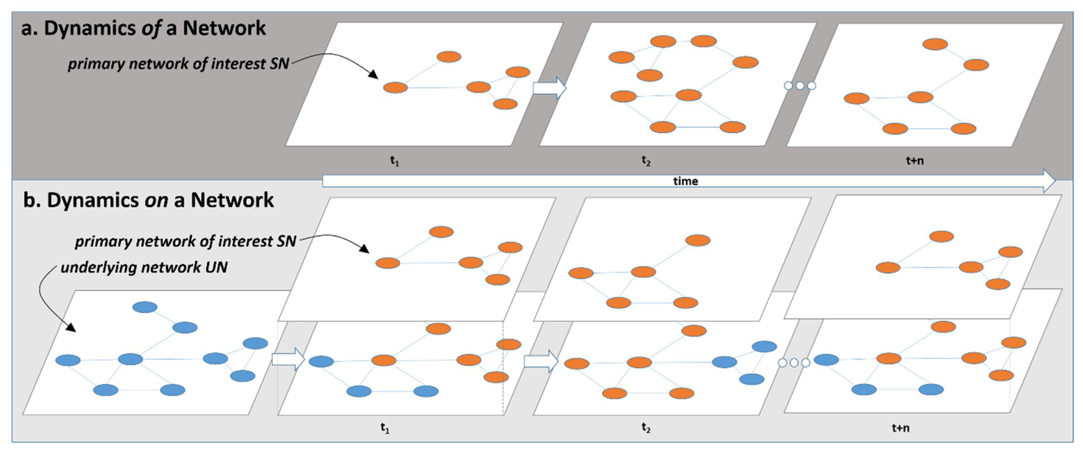
As demonstrated in the example above, it is often the case that a spatial network of primary interest SN is formed based on an underlying network UN (Figure 1a) where UN is the underlying network, SN is the spatial network, J is the defined neighborhood, R are the transition rules, C is the connection cost, and t is the time increment of the GNA model. This type of GNA can be defined by expression (1).
In the less common case where there is no underlying network UN and the network evolves as a function of its own structure (Figure 1b), a spatial network of interest SN is formed independent of an underlying network. Therefore, the GNA expression (1) is modified and presented as:
Both the evolving spatial network SN generated by the GNA and the underlying network UN is composed of a set of nodes N representing components of a system. Pairs of nodes are connected by links L, representing interactions or relationships between system components. The spatial network SN can be expressed as:
An underlying network UN can also be expressed as:
The sets of nodes N and links L in the spatial network SN or underlying network UN are further expressed as:
Each node v and link e in the set of nodes N and links L are defined by several spatial, non-spatial, and network properties (Table 2). Nodes N are defined by their spatial properties, most importantly geographic location which in turn facilitates the measurement of geographic distance d between any two nodes. Depending on the type of phenomenon that the set of nodes represent, other geometric properties such as area and perimeter may be of interest. Nodes N are also defined by network properties such as the number and list of connections a node v has to other nodes in the network or node weight. A weight is a value that is assigned to a node and can be used to quantify the magnitude of flow, importance, suitability, or preference within a set of nodes N.
Links L are also defined by their spatial properties, which differ slightly from the spatial properties of nodes. Whereas nodes N are always embedded in geographic space, in most cases, links L are not. The exception is a planar network such as a road network, in which case the link length is of interest. Links also contain the important network property of link weight, which can be used to quantify the magnitude of flow of individuals, materials, or information between nodes. Links are either unidirectional or bidirectional, meaning that flow occurs in one or both directions respectively. Both nodes N and links L have non-spatial properties which are qualitative or quantitative attributes used to describe the network node or link.
Transition rules R are designed to represent the real-world dynamics between system elements and determine the evolution of the spatial network SN. Transition rules are in most cases applied to node ’s neighborhood J, defined as the set of nodes connected to node in some way. The development of transition rules R depends on whether the spatial dynamics are represented on a network or of a network. In the case of representing dynamics on a network, transition rules R may be defined where the spatial network SN interacts with the underlying network UN. For example, at time step t, node in the SN forms a link to node in the UN if node has some weight. The nodes that meet these conditions make up node ’s neighborhood J. In the case of representing dynamics of a network, the development of transition rules R depends on interactions between nodes within the SN. For example, at time step t, if there are less than three nodes within a certain proximity to node , a new node is spawned within this proximity and a link forms between node and node . The nodes that meet these distance-based conditions make up node ’s neighborhood J. Connection cost C evaluates the resistance of the geographic space between nodes to both the formation of links between nodes or to the generation of new nodes. This space between nodes is referred to as the cost matrix. Resistance in this context may be a function of distance between nodes or the low suitability of the matrix for connecting nodes or the spawning of new nodes.
The spatial and topological organization of the spatial network SN and in some cases the UN, specifically what nodes are connected to what nodes using which links, are recorded in the NxN adjacency matrices ASN and AUN, respectively. In these tables, the existence of a link between two nodes in a network is recorded using a value of 1, with the alternative recorded using a value of 0.
In the case of simulating dynamics on a network, applied transition rules R and connection costs C influence the underlying network UN, which in turn influences the spatial network SN and thus alter the information recorded within the adjacency matrices at each time step. Therefore, spatial network SN evolution with each time step is defined where the adjacency matrix at the subsequent time step t + 1 is a function of the underlying network UN, the neighborhood J, the generative rules R, the connection cost C, and the adjacency matrix at the previous time t. In the case of simulating dynamics of a network, applied transition rules R and connection costs C alter the spatial network SN and thus alter the information recorded within the adjacency matrix at each time step. Therefore, the spatial network SN evolution is defined where the adjacency matrix at the subsequent time step t + 1 is a function of the neighborhood J, the generative rules R, the connection cost C, and the adjacency matrix at the previous time t.
2.2. GNA Spatial Network Analysis using Graph Theory
The output of a GNA is a sequence of evolving spatial networks of primary interest SN representing a real-world phenomenon over space and time. This representation is useful because the structure of spatial networks can be characterized using graph theory measures [24,25,26,27]. The structural and dynamical properties of real-world networks often exhibit some or many of the same properties of four well-defined theoretical graph types: regular, random, small-world, and scale-free. These types of graphs can be distinguished from one another using a few simple global graph theory measures including average degree <k>, degree distribution P(k), average clustering coefficient <C>, and average path length <l> (Table 3). Each type of graph can be considered in a non-spatial or spatial context. In a non-spatial context, the location of nodes is of no concern, but instead, the way in which nodes are connected to other nodes. In a spatial context, nodes have a location in geographic space.
Networks that exhibit properties of regular graphs are composed of a set of nodes and links, where each node has the exact same number of links of degree k [28]. A regular graph that is non-spatial is presented in a way that does not consider the spatial location of nodes, but rather is concerned with the way in which the nodes are connected. For example, nodes might be arranged in a circle where each node is connected to its neighboring nodes. The circular arrangement is spatially meaningless, but rather is selected for better understanding of the topology of the graph. A spatial regular graph may be arranged so that its georeferenced nodes are organized in a manner where all links are of the same length d and all nodes have the same degree k. In either case, since all nodes are tightly connected to their nearest neighbors, both non-spatial and spatial regular graphs have a high clustering coefficient <C>. The localized connections result in a longer average shortest path length <l> between pairs of nodes in the network.
Unlike regular graphs, properties of non-spatial random graphs differ significantly from random spatial graphs. Networks that exhibit the properties of random graphs that are non-spatial are composed of nodes that are connected to other nodes at random [29]. As the graph is non-spatial, connections between nodes are not influenced by the distance between them. Random graphs that are non-spatial are defined by a degree distribution P(k) where all nodes have a similar degree k. This well-defined average degree produces a Poisson degree distribution P(k). Since any two nodes are connected at random, the average clustering coefficient <C> and the average path length <l> are very small. A non-spatial random graph is also known as an Erdos–Renyi (E-R) graph after the two mathematicians who first introduced the concept of random graphs.
There are two main types of random spatial graphs. The first type is referred to as a random geometric graph (RGG), composed of nodes that are randomly located in geographic space. Unlike a non-spatial random graph, nodes in an RGG are not connected randomly, but rather connect to other nodes if the distance between the two nodes falls within a selected distance threshold d [30]. The distance threshold d can be defined using Euclidean, Manhattan, or geodesic distance [31]. The properties of RGGs differ from traditional non-spatial random graphs because the distance threshold produces localized clustering between adjacent nodes and a lack of long-distance connections, characteristic of many spatially embedded real networks [25]. The inclusion of geographic space as a constraint in network structure provides more realistic representations of real phenomena than non-spatial networks. Thus, RGGs have been used as a model to better understand many types of real phenomena ranging from telecommunication networks to social networks. A second type of random spatial graph is referred to as a spatial E-R graph. In this representation, nodes are distributed randomly in geographic space and are connected at random based on the probability p.
Small-world graphs, both their non-spatial and spatial counterparts, are characterized by a structure that falls between regular graphs that have no randomness at all and random graphs that are entirely random [32]. Like a regular graph, the majority of nodes in small-world graphs are connected to their nearest neighbors, however a few nodes are connected to distant nodes. This type of graph also produces a Poisson degree distribution P(k) when graphing the degree distribution as a histogram. However, small-world graphs are different than regular or random graphs because the few distant connections between nodes produce a high average clustering coefficient <C>, but dramatically reduce the average path length <l>. Social networks typically exhibit properties of small-world graphs, where there exist only a few intermediate acquaintances between any two people in the world. Dynamics on a small-world network such as the passing of information or a virus is highly efficient. Specifically, because of this short average path length <l> the passing of information or the spreading of a virus from node i to node j can occur with just a few intermediaries.
Networks, either non-spatial or spatial, with properties characteristic of scale-free graphs typically have a degree distribution P(k) where a few nodes have a disproportionately large degree and the majority of nodes have a very small degree [33]. This produces a scale-free degree distribution with a low average clustering coefficient <C> and a small average path length <l>. Barabasi and Albert (1999) refer to networks with power-law distributions as “scale-free” networks because the same power-law distribution remains across all scales in the network. This network structure is explained by growth and preferential attachment, meaning that as the network forms, the probability that a new link will be added to node is proportional to the degree k of that node and can result in the formation of hubs with an anomalously large number of links. These types of network are robust to random attack, however, the loss of a hub in a targeted attack would cause system failure [34]. Node degree is not the only factor contributing to preferential attachment [35] and several modifications have been proposed where the probability that a new link will be added to node is proportional to node age [36,37].
Global graph theory measures can be used to characterize the overall network structures, to give insight into spatial dynamics that take place on those structures, to compare between different systems, and to compare between the same system as it evolves over time. Some important global graph theory measures are presented in Table 3 that provide a complete snapshot of network structure that includes but are not limited to number of nodes n, number of links m, average degree <k>, degree distribution P(k), average clustering coefficient <C>, and the average shortest path length <l>. These particular measures are used to characterize the network structures produced by the GNA models presented in the following sections.
3. Geographic Network Automata Case Studies
In the following sections, the application of the proposed GNA framework to the spatially explicit network version of the Game of Life GNAGOL and Schelling’s Segregation GNASEG is presented. Both models are developed using the Java programming language in the Eclipse integrated development environment using the REcursive Porous Agent Simulation Toolkit (Repast) [38].
3.1. GNA Game of Life GNAGOL
The Game of Life is selected as the first case study to present the GNA framework because it is a well-known model of a theoretical system that is inherently simple and operates in space and time. The original Game of Life is a cellular automaton developed by John Conway in 1970 that was designed to simulate dynamics of reproduction, death, and survival of cells in a lattice. Applying these dynamics to nodes in a network permits the exploration of spatial network evolution, specifically spatial network growth and shrinkage as nodes are added and removed over time. Therefore, this case study facilitates broader learning about spatial network dynamics and evolution.
3.1.1. GNAGOL Modelling Framework
The GNAGOL model simulates an evolving spatial network SN which is constrained to an underlying random geometric graph (RGG) network UN. Based on the expression (1), the GNAGOL can be presented as:
where the GNAGOL is a function of the underlying network , the spatial network of interest , the neighborhood J, the transition rules , the connection cost , and time .
The underlying RGG UNGOL is static where a set of nodes N are located randomly in geographic space and the total number of nodes n = 2000. The number of nodes n was chosen to demonstrate the GNA methodology. Node and node in the set of nodes N are connected by a link and thus are considered neighboring nodes if the Euclidean distance dij between them is less than 1 km. The given range for d defines the neighborhood J for each node. As the spatial distribution of all nodes is random rather than a regular tessellation, nodes in the UNGOL do not have the same number of neighboring nodes. This differs from the traditional formulism of the CA version of the Game of Life which operates on a regular spatial tessellation where all cells have the exact same number of neighbors. Each node in the set of nodes N can be defined by its location (x, y coordinates), the distances d between its neighboring nodes, and its “alive” or “dead” state. Lastly each node is defined by its local network properties including its degree k, clustering coefficient C, and shortest path length l.
The spatial network SNGOL is composed of nodes with the same spatial and network properties, however, nodes in this network can only be in the “alive” state. Transition rules representing dynamics of reproduction, death, and survival are applied underlying network UNGOL where nodes are added, removed, and rewired over time, thus producing an evolving spatial network of “alive” nodes SNGOL that can be analyzed. There are four transition rules R based on the Game of Life [20], which are applied to the UNGOL at time t and determine the UNGOL and the SNGOL at time t + 1, as follows:
R1—to simulate the dynamics of underpopulation, any live node with some number or fewer of alive neighbors j dies and is removed from the spatial network SNGOL;
R2—to simulate the dynamics of survival of the fittest, any alive node with exactly some number of alive neighbors maintains their alive state and thus their place in the spatial network SNGOL;
R3—to simulate the dynamics of overpopulation, any alive node with some number or more of alive neighbors j dies and is removed from the spatial SNGOL;
R4—to simulate the dynamics of reproduction, any dead node with exactly some number of alive neighbors, j becomes an alive node and is added to the spatial network SNGOL.
Although the influence of the cost matrix on system dynamics is not formally explored in the traditional Game of Life, a barrier is introduced into the GNAGOL to demonstrate the use of the connection cost C in the GNA framework. The connection cost C is as follows:
C1—a link cannot form between node and node if it intersects the barrier
For any model run, the underlying network structure UNGOL is always the same, although the states of the nodes change. The UNGOL and subsequently the SNGOL are initialized at time t0 where 50% of the 2000 nodes are randomly selected as “alive”. The underlying network UNGOL in the GNAGOL implements a synchronized node update process. First, the number of alive neighboring nodes is calculated for each node in the underlying network UNGOL. Second, the transition rules R are applied and the state of each node changes based on its number of live neighbors. Finally, the new number of alive nodes is calculated. If the node is alive, the node stays or becomes part of the spatial network of interest SNGOL and connects to its live neighbors. The GNAGOL is run for 20 time-steps after which the evolving spatial network SNGOL reaches equilibrium and the majority of the nodes are satisfied.
3.1.2. GNAGOL Scenarios
Two scenarios were developed by adjusting the transition rules R1–R4 of the GNAGOL model to represent different spatial behaviors simulated using evolving spatial networks SNGOL. Scenario 1 uses transition rules R presented in Table 4 to generate a spatial network that grows and expands over time. To foster a growing network, rules are calibrated so that having more neighbors is desirable i.e., parameter x is selected in a way that reproduction and overpopulation is encouraged while underpopulation is discouraged. Scenario 2 uses the transition rules R presented in Table 4 to generate a spatial network that shrinks and declines in size over space and time. To foster a shrinking network, rules are calibrated so that having less neighbors is desirable i.e., parameter x is selected so that reproduction and overpopulation is discouraged and underpopulation is encouraged. In both scenarios, the connection cost C1 remains the same, where a link cannot form between node and node if it intersects the barrier. There are several real-world examples of systems as networks that may exhibit these types of spatio-temporal behaviors. A growing network, where the number of nodes and links increases consistently over time can be representative of any type of diffusion-based phenomena like spread of invasive species, transmission of disease, spread of computer viruses, urban sprawl, flooding, and communication networks. A shrinking network, where nodes are continuously removed from the network may be representative of processes such as deforestation, loss of habitat due to invasive species, loss of agricultural land, and drought. The GNA is not limited to simulating these two types of network evolution since network evolution emerges from implemented transition rules intended to represent location dynamics between nodes. One other general type of network evolution might be network fluctuation as some parts of the network grow while simultaneously other parts of the network shrink.
3.1.3. GNAGOL Results
The output of the GNAGOL is a series of spatial networks SNGOL that evolve as a function of transition rules R that are applied to the underlying network UNGOL. Specifically, the measured evolving network SNGOL structure is limited by the underlying random geometric graph (RGG) structure UNGOL and thus the GNAGOL in both scenarios produce an evolving spatial network SNGOL that is also an RGG. The structure of the underlying network UNGOL does not allow for the emergence of a spatial network of interest SNGOL that has properties of other graph types such as scale-free or small-world. Based on the random evolving spatial network structure SNGOL produced by the GNAGOL, the network structures observed and measured here characterize RGGs as they respond to dynamics that cause growth and shrinking responses. As many types of real phenomena are represented and modelled by RGGs, it is important to understand how processes that operate on the RGG structure might be impacted by changes in their structure. In the following section, the obtained GNAGOL simulation results are presented and the evolving spatial network SNGOL is analyzed using graph theory measures.
GNAGOL Simulation Results
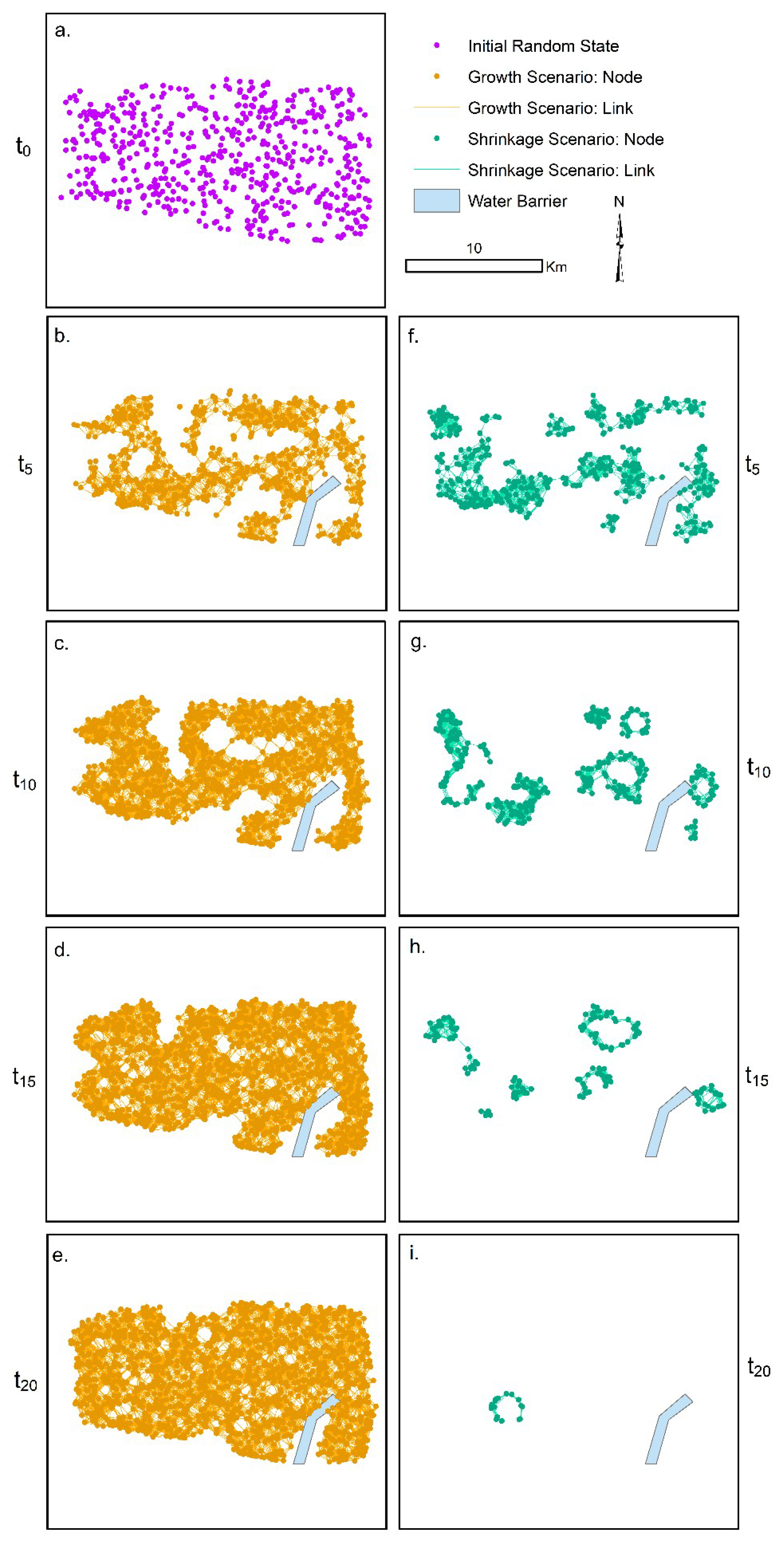
The obtained simulation results from both scenarios are presented in Figure 2. In both scenarios, following initialization, 50% of nodes are selected randomly as “alive” (Figure 2a).
Scenario 1—the application of the transition rules R developed to simulate spatial network growth initially forms a configuration that is composed of thick clusters of nodes (Figure 2b). Since the transition rules R create an imbalance in favor of node reproduction (R4) and survival (R2), the clusters expand over time as “dead” nodes close to the edge of clusters eventually have enough “live” neighbors that are required for them to reproduce and join the spatial network SNGOL (Figure 2c–e). As such, the network as a whole grows over time as if “spreading”. Chain and loop-like structures form as the interiors of each cluster die from overpopulation and the exteriors of each cluster die from underpopulation, leaving the rest of the nodes in the cluster with the correct number of links survive until the next time step. The loop-like configurations and the repeating patterns are like that of the patterns that are produced in the original version of the Game of Life.
Scenario 2—the application of the transition rules R developed to simulate spatial network shrinkage initially forms a sparse set of clusters, where some clusters are connected to the larger spatial network and others are not (Figure 2f). This is a result of the transition rules R that are designed to reduce node reproduction and eliminate node survival. As a result, the network quickly shrinks until the network is reduced to a repeating sequence of relatively stable loop-like configurations (Figure 2g–i). As soon as a configuration is produced that is unstable, resulting in the loss or gain of nodes, the network collapses and all nodes die from underpopulation.
GNAGOL Spatial Network Analysis Results
General Trends—the evolving spatial network SNGOL is characterized by the number of nodes n, number of links m, the average clustering coefficient <C>, the average degree of alive nodes <k>, and average path length <l> calculated for each iteration for scenario 1 (Figure 3a) and scenario 2 (Figure 3b). In general, in scenario 1, the network grows steadily in size over time. The rate of growth is faster in early time steps and slows in later time steps as the network finds a stable configuration and less dead nodes are available to reproduce and join the network as live nodes. In scenario 2, the network decreases in size over time with only a few time steps where the number of nodes increases slightly before then decreasing. The results indicate that the network measures collected for the shrinking network (Figure 3b) are noisier than the network measures collected for the growing network (Figure 3a). In the growing network, in all time steps, the number of nodes and links is greater than in the previous time-step. In the shrinking network scenario, in some time-steps, the number of nodes and links increase before sharply decreasing. This noise is a function of applying the rules for overpopulation. Nodes survive, reproduce, and rewire to other nodes. As their degree increases over time, it surpasses the struct threshold set by R3 and then dies in the next iteration.
Correlations between Graph Theory Measures—Table 5 presents the correlation between graph theory measures obtained from the generated spatial networks in scenario 1 (Table 5a) and scenario 2 (Table 5b).
Scenario 1: based on the results presented in Table 5a, the growing spatial network SNGOL structure exhibits a strong positive correlation between number of nodes and the number of links, average path length, and average degree. Conversely, there is a strong negative correlation between average clustering coefficient and the number of nodes, number of links, average path length, and average degree.
Scenario 2: the shrinking network structure SNGOL exhibits strong to moderate positive correlations between the number of nodes and the number of links, average, path length, and average degree (Table 5b). There is a moderate to weak negative correlation between average clustering coefficient and the number of nodes, number of links, average path length, and average degree.
In general, for the evolving spatial networks SNGOL simulated in all scenarios, as RGGs grow in size, the number of links, the average path length, and the average degree increase while the clustering coefficient decreases. Conversely, as RGGs shrink, the number of links, the average path length, and average degree also decrease, while the clustering coefficient increases. These findings support conclusions that graph theory measures are dependent on network size [39]. These correlations are particularly interesting because the relationship between network size and other graph theory measures are not well understood and rarely explored in the literature, especially in the case of spatially explicit networks.
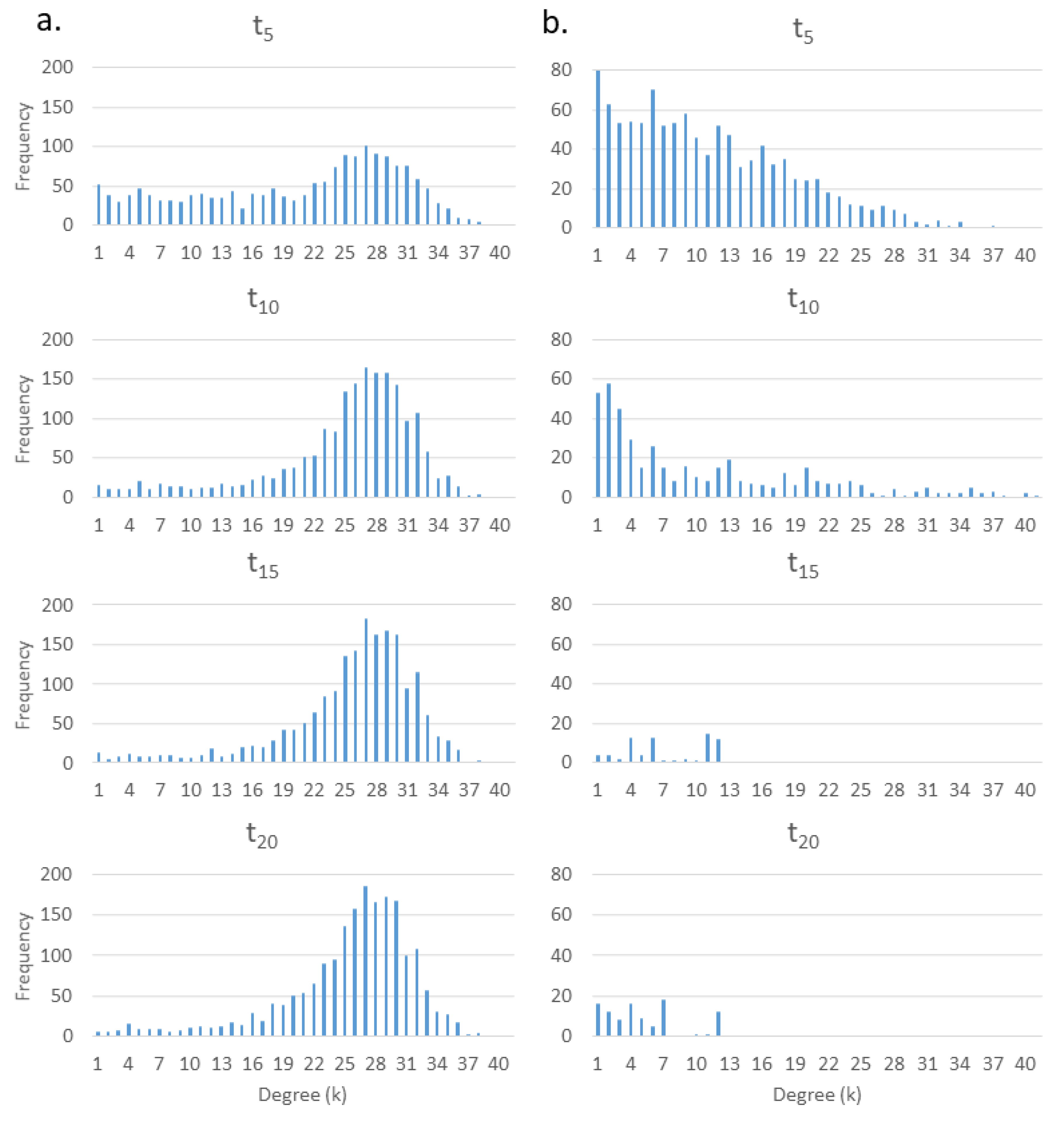
Degree Distribution. When an evolving network undergoes growth (scenario 1) and network size increases, node degree increases, which produces a degree distribution with a left negative skew (Figure 4a). When an evolving network undergoes shrinkage (scenario 2), nodes are removed, leaving remaining nodes with a smaller degree, producing a degree distribution with a right positive skew (Figure 4b).
The Game of Life is a well-known model of a theoretical spatial system selected as a case study to demonstrate clearly the GNA modelling framework, however the presented GNAGOL does not incorporate real geospatial datasets. In the case of a geospatial application of the GNA modelling framework to real-world phenomena, the elements of the GNA including the initial network state, the underlying network, the transition rules, the connection cost, and the spatial and temporal resolution would need to be designed to properly reflect a particular real-world system and include geospatial data to permit GNA development, calibration, sensitivity analysis to initial conditions and parameters, and validation. This process would be the same for designing any cellular automaton or for an agent-based model. In the following section, a second model that incorporates real geospatial data into the GNA modelling framework is presented.
3.2. GNA Schelling’s Segregation GNASEG
Schelling [21,22] has presented a model that was able to capture spatial patterns of human segregation, the self-organization of heterogeneous individuals into clusters of “alike” individuals, using one rule. This rule is as follows: if an individual is dissatisfied with the composition of others that live within its neighborhood, the individual moves elsewhere until it is satisfied. This rule provides a way to model highly complex social processes that pull people together based on similarities in language, interests, gender, ethnicity, careers, political views, education, language, and so on. Shelling’s work has been extended to explore the effects of parameter adjustments including individual tolerance, neighborhood size, population structures, and utility functions driving segregation [40,41]. In other research studies, models are parameterized based on real data [42,43,44]. In many cases, segregation is modelled as networks [45,46,47,48], however, network representation and analysis of the spatial processes of segregation using real geospatial data has not been explored.
In this section, a second GNA is developed. The GNASEG model is a prototype for representing patterns of segregation in an urban environment. The model presented is more advanced than the GNAGOL model as it incorporates real geospatial data forming an underlying network, accesses several node neighborhood types for which the transition rules are implemented, and explores dynamics between several different node types. In this network, unlike the GOL, the network evolution is not characterized by addition or removal of nodes, but rather the rewiring of a similar number of nodes change location over time.
3.2.1. GNASEG Modelling Framework
The GNASEG model simulates an evolving spatial network SN which is constrained to an underlying spatial network UN of urban residential properties. Therefore, based on the expression (1), the GNASEG can be presented as:
where the GNASEG is a function of the underlying network , the tightly coupled spatial network of interest , the neighborhood J, the transition rules , the connection cost , and time increment .
The underlying spatial network UNSEG is constructed where total number of nodes n = 20,213. Each node in the set of nodes N represents the actual location of unoccupied residential properties located in several neighborhoods in the City of Vancouver, Canada including the West End, Downtown Vancouver, Hastings Sunrise, Strathcona, and Grandview Woodland. The location of the properties is obtained from real geospatial data produced by the City of Vancouver and can be characterized as having a clustered spatial pattern. Residential properties in only a few Vancouver neighborhoods are included in the study and thus limit the number of nodes n in order to maintain computational efficiency. In the underlying spatial network UNSEG, node and node in the set of nodes N are connected by a link and thus are considered neighboring properties if the Euclidean distance dij is smaller than a given neighborhood J range, in this case dij <= 50 m. The value for the neighborhood was selected by calculating the average nearest neighbor distance in meters. Since the neighborhood is defined by proximity, the graph is considered a geometric graph. However, because the nodes are not distributed randomly in geographic space, the underlying network is not considered an RGG.
For any model run, the underlying network structure UNSEG is always the same. Each node and link in the set of nodes N and links L for the underlying spatial network UNSEG can be defined by its spatial properties including location (x, y coordinates) and the distances d between other nodes. Each node can also be characterized by its state “occupied” or “unoccupied”. Lastly each node is defined by its local network properties, where each individual node has a degree k, a clustering coefficient C, and a shortest path length l.
The spatial network SNSEG is composed of nodes representing the location of families that occupy the properties in Downtown Vancouver. It is assumed that only one family occupies each property. Nodes in the spatial network SNSEG have the same spatial and network properties as the underlying network UNSEG, however, nodes have two states of either “Class A” or “Class B”. Node and node in the spatial network are connected by a link if dij <= 50 m. The SNSEG is initialized at time t0 where of the 20,213 nodes representing residential properties, 33% are vacant, 33% are occupied by Class A, and 33% are occupied by Class B. The initial allocation of families to properties that are of Class A or Class B is equally likely.
The spatial network SNSEG emerges from segregation dynamics between neighboring family nodes in the spatial network SNSEG and unoccupied property nodes in the underlying network UNSEG. Furthermore, the spatial network SNSEG is limited by the availability of properties in the underlying network UNSEG. There are two transition rules R, which are applied at time t and determine the SNSEG at time t + 1. For their implementation, two types of neighborhoods J are considered. Neighborhood JA only considers the neighboring family nodes of family node contained in the spatial network SN. Neighborhood JB only considers the neighboring occupied and unoccupied property nodes of family node in the underlying network UNSEG. The transition rules R are as follows:
R1—based on the definition of neighborhood JA, if node ’s neighborhood is composed of a higher ratio of neighbors of the opposite class, the node is dissatisfied and moves to a new unoccupied location.
R2—based on the definition of neighborhood JB, if node ’s neighborhood is composed of a higher ratio of unoccupied properties than occupied properties, the node is dissatisfied and moves to a new unoccupied location.
Each property node in the underlying network UNSEG keeps track of its neighboring property nodes, whether they are unoccupied, occupied by Class A, or occupied by Class B. This information is used by the family node to understand the neighborhood’s composition and to determine whether it is satisfied with its location or not. The GNASEG is run for 20 time-steps, after which the model reaches equilibrium and the majority of agents are satisfied meaning that there is little movement beyond 20 time-steps.
3.2.2. GNASEG Results
The GNASEG outputs consist of a series of spatial networks SNSEG that evolve as a function of the transition rules R that are applied to the spatial network SNSEG as well as the interactions between the SNSEG and the UNSEG. In the following section, simulation results for the obtained GNASEG are presented and the generated evolving spatial network SNSEG is analyzed using graph theory measures.
GNASEG Simulation Results
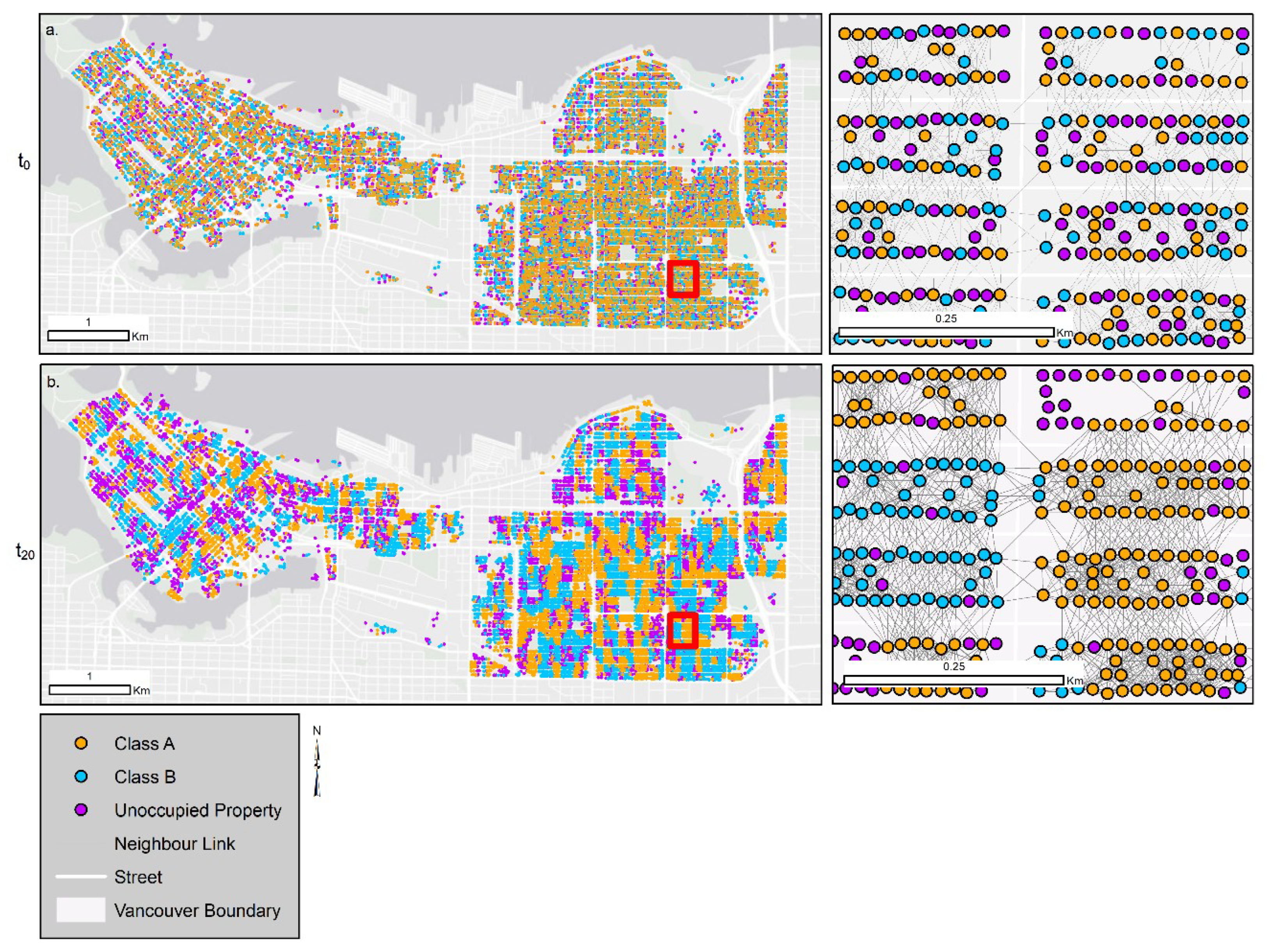
The obtained simulation results from the GNASEG are presented in Figure 5. The model is initialized at time t0 where one third of the residential properties in the selected Vancouver neighborhoods are assigned at random as being occupied by Class A, one third of the residential properties are assigned at random as being occupied by Class B, and one third of the residential properties remain unoccupied (Figure 5a). The inset map for Figure 5a shows in detail the random composition of the classes several city blocks and how they are connected. At time t20, nearly all the nodes are satisfied with their location (Figure 5b). The inset map for Figure 5b shows the no longer random geographic distribution of nodes, but instead, properties that are in proximity are occupied by nodes of the same class.
GNASEG Spatial Network Analysis Results
General Trends—the evolving spatial network SNSEG can be described as not shrinking or growing, but re-wiring, meaning the connections between nodes change over time as nodes change location. The spatial network SNSEG is characterized by the following graph theory measures: the number of nodes n, number of links m, average clustering coefficient <C>, average degree of nodes <k>, average path length <l>, and assortativity, calculated for each time step (Figure 6). Assortativity measures the degree to which connected nodes are alike, in this case, the degree to which nodes belonging to Class A are connected to Class A and vice versa. If the assortativity for the network is 1, nodes are only connected to nodes of the same class. Thus, the graph theory measure assortativity is capable of quantifying the degree of segregation in the spatial network and is useful because it summarizes all spatial interactions across the entire study area.
In general, the number of nodes connected to the spatial network SNSEG slightly decreases over time as some nodes move to locations with no neighbors at all and become satisfied. Conversely, the number of links increases over time. This can be explained whereby, initially, city blocks composed of many properties contain several unoccupied properties (Figure 5a inset). Unoccupied properties are not connected to the spatial network SNSEG, they instead make up the underlying network UNSEG. This reduces both the average degree and the clustering coefficient of occupied properties because many neighboring residential properties in close proximity to a node are unoccupied. Based on the transition rule R2, family nodes in the spatial network SNSEG are dissatisfied if there are more unoccupied properties than occupied properties in their neighborhood. Therefore, over time, the clusters of homogenous occupied urban residential properties and clusters of unoccupied properties form (Figure 5b inset). As some city blocks no longer contain any unoccupied properties, the degree and the clustering coefficient of these nodes increase. As a result of this behavior, the average clustering coefficient and average degree of the spatial network SNSEG increase over time, decreasing the average path length. Finally, assortativity increases significantly over time from 0.0 to 0.7 as the network becomes increasingly segregated.
Correlations between Graph Theory Measures—Table 6 presents the correlation between graph theory measures obtained from the generated spatial networks SNSEG. It is important to note that some of the correlations between the graph theory measures are a function of the spatial dynamics that take place on the network. For example, segregation processes increase assortativity and simultaneously increase the average clustering coefficient, which in turn creates a strong positive correlation between these two measures.
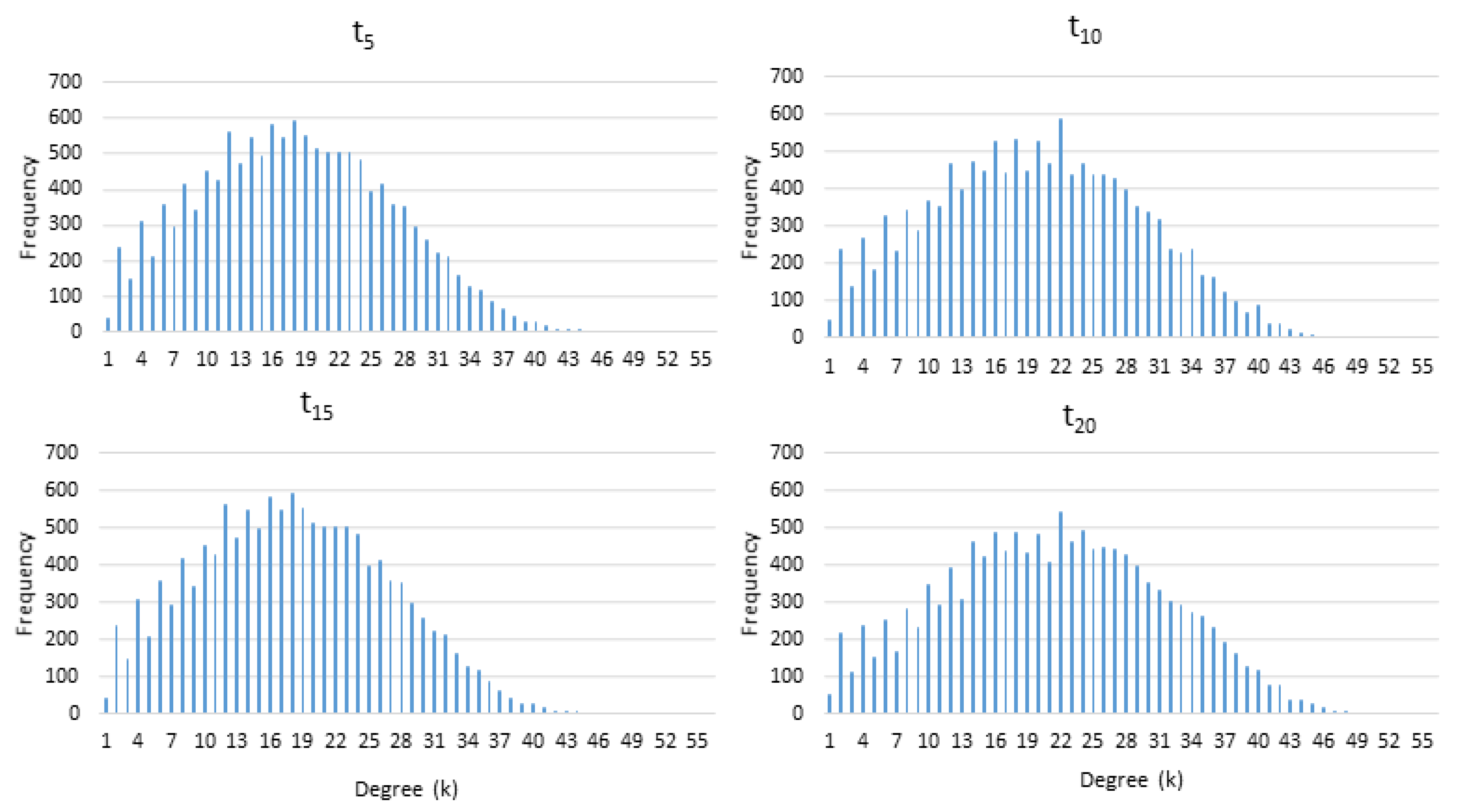
Degree Distribution—the degree distribution is a Poisson distribution and remains relatively stable as the spatial network SNSEG changes over time. Specifically, the degree distribution for t5, t10, and t15 is characterized by an index of dispersion of 0.98. The degree distribution is initially slightly skewed to the right before becoming more normal with an index of dispersion of 0.99 as the average degree increases slightly as presented in Figure 7.
When comparing the obtained results for the two case studies, the number of nodes and the number of links are strongly negatively correlated in the spatial network SNSEG and are strongly positively correlated in the spatial network SNGOL. This is a function of the transition rules in the spatial network SNSEG that force the re-wiring of the network to a configuration with more links that better satisfies a lesser number of family nodes. Furthermore, the SNSEG is not an RGG since the nodes are not organized randomly, but are instead clustered. Despite these differences between the network types, there are four correlations that hold true in both GNA case study model outputs. In all networks produced by both models, (1) the number of nodes and average clustering coefficient is strongly negatively correlated, (2) the number of nodes and average path length is positively correlated, (3) the number of links and average degree is strongly positively correlated, and (4) the average path length and the average clustering coefficient is strongly negatively correlated. The developed GNASEG is a model designed for the purpose of presenting the GNA modelling framework that implements a real geospatial dataset. The developed GNASEG prototype is highly scalable and thus provides a starting point that would facilitate easy parameterization using additional real data in the future.
4. Discussion and Conclusion
This study introduces the novel modelling framework of Geographic Network Automata (GNA) that can be used for the representation and analysis of complex spatio-temporal systems as evolving and dynamic networks. The proposed GNA modelling approach presented in this study fits within the larger modelling framework of geographic automata systems (GAS) [49,50], a suite of geographic modelling approaches that includes cellular automata (CA) and agent-based modelling (ABM). GAS modelling frameworks seek to capture the complexity inherent to real geographic phenomena by simulating local level interactions from which system-level behavior emerges. While the GNA discretely represent interactions between nodes using links, CA represent local dynamics between cells [51] and ABMs represent interactions between individuals or “agents” [52,53]. Like the proposed GNA modelling approach, CA and ABM under the GAS theoretical framework are coupled with geographic information systems (GIS) and geospatial data sets and have been used to model a variety of real geographic phenomena with early studies in urban [54,55], social [56], and ecological systems [57]. The addition of the proposed GNA modelling approach helps to better theoretically situate other modelling approaches that are in some ways “hybrids”, including for example graph-cellular automata [58] and network-based ABMs [59,60,61].
While the proposed GNA modelling approach fits well within the framework of GAS, it maintains a strong departure from the classic cell-based CA and vector-based ABM. The developed GNA approach is designed to explicitly leverage network representations, network-based neighborhoods, network-based transition rules, and network analysis using graph theory for the simulation of complex spatio-temporal phenomena. The GNA modelling framework differs from traditional GAS including CA and ABM because of its uniquely explicit view of the network-based relationships and interactions between the spatial features that is represented by links and the NxN adjacency matrix A. The GNA modelling framework places emphasis on the representation, analysis, and visualization of relational data, interactions, and flows.
In CA and ABMs, transition rules are implemented to simulate relationships, interactions, and flows, but they are not often represented explicitly nor measured discretely. Instead, the way in which the system responds to these interactions is measured. The GNA offers a more flexible modelling framework than traditional CA where nodes may be mobile, may have several defined neighborhood types for which the transition rules are implemented, and non-deterministic system-level behavior. Furthermore, the GNA offers explicit representation of interactions as links and thus provides “X-ray” vision of the model that can be used for measuring and visualizing large sets of interactions between components of a system in a way that ABMs traditionally do not.
“Networks are everywhere” is a phrase found in many studies that review network research that ultimately speaks to the interdisciplinary nature and usefulness of abstracting real systems into complex spatial dynamic networks. This speaks to the potential for the GNA to be implemented on many other geospatial applications for the representation, characterization, and analysis of a variety of complex systems. Complex spatial networks are a natural fit for representing and analyzing relationships and interactions and as such, the GNA modelling framework is an ideal approach for applications when interaction, relationships, dynamics, and flows between sets of components are of interest. The application potential is vast and includes movement and flows of information, people, resources, money, ecological species, energy, disease, and transportation vehicles over time and across points in geographic space. Naturally, the study of spatial and non-spatial relationships between individuals is also an ideal application for these modelling approaches. In addition, the proposed GNA modelling approach would be ideal to better understand interactions between two or more tightly coupled systems over space and time such as interactions among policy, social, and environmental systems. The proposed GNA modelling framework was not developed with the intention to replace other GAS nor does it claim to be better than, but instead, offers novel means for representation and a new lens for analysis of complex spatio-temporal phenomena.
The presented GNA models successfully represent dynamic spatial phenomena as networks as demonstrated using the two case studies. The quantification of the simulated network structures using network measures can reveal new understanding of the phenomena. In the Game of Life example, the network measures offer a way to quantify common behaviors of spatio-temporal phenomena such as growth and shrinkage. In the segregation example, it is revealed that the network measure assortativity can be very useful for quantifying segregation at the individual level and as a whole. This has been a challenge with traditional segregation indices which tend to summarize segregation within various units of measure i.e., census boundaries and as such are subject to the modifiable areal unit problem.
The Game of Life GNAGOL example presented in this research study, simulates the evolution of network structures composed of nodes that are geographically referenced. The segregation GNASEG example uses real GIS data for the study area in City of Vancouver to represent the actual location of nodes where each node represents a residential property in the city. There is a qualitative difference between the two case studies where the level of GIS integration is increased from the GNAGOL to the GNASEG. Integrating GIS and network automata and thus providing the framework of geographic network automata are advantageous in three ways: (1) the network structure and dynamics can be linked to georeferenced data representing real world phenomena, (2) the geovisualization of simulated evolving spatial networks are georeferenced to a study area, and (3) both the spatial analysis using GIS and network analysis of the generated spatial network structures can be leveraged.
Even though the GNASEG incorporates actual spatial data to form the underlying network UNSEG, future work may focus on additional parameterization and full model testing and validation. Model validation is seen as the degree of agreement between simulated spatial network structures and observed real-world spatial patterns, which should be evaluated using datasets that are independent of model development and calibration. Future work would require the exploration of model validation approaches suitable for comparing evolving networks with real datasets even in the face of data scarcity like the NEAT validation approach [62].
In conclusion, this study presents geographic network automata (GNA), a modelling approach developed for the simulation of spatial systems as evolving complex spatial networks. The novelty of the GNA approach lies in its ability to represent the tight coupling between spatial network structure and network dynamics, resulting in network space–time evolution. The GNA approach acknowledges that for many phenomena network evolution occurs in geographic space, and thus geospatial data and geographic information systems can be leveraged for representing and analyzing real systems. The GNA modelling framework adopts a complex systems approach by simulating local spatial interactions between georeferenced nodes represented by links from which a complex network emerges. Ultimately, this approach is a new class of GAS alongside ABM and CA models. The framework is implemented using a spatial network representation of two GNA models including Conway’s Game of Life and Shelling’s Segregation Model where the implemented transition rules simulate dynamics between nodes at the very local level, altering the structure of the spatial network, which in turn influences the dynamics between nodes. Graph theory is then used to characterize and measure the structure and behavior of simulated networks. The developed GNA approach is both general and flexible so that it can be applied to represent and analyze many real geographical systems including urban, social, and ecological and has the potential to be used in knowledge discovery and decision-making processes.
Author Contributions
Conceptualization, Taylor Anderson and Suzana Dragićević; Formal analysis, Taylor Anderson; Funding acquisition, Taylor Anderson and Suzana Dragićević; Investigation, Taylor Anderson and Suzana Dragićević; Methodology, Taylor Anderson; Resources, Suzana Dragićević; Supervision, Suzana Dragićević; Visualization, Taylor Anderson; Writing—original draft, Taylor Anderson; Writing—review and editing, Suzana Dragićević. All authors have read and agreed to the published version of the manuscript.
Funding
This research was funded by Natural Sciences and Engineering Research Council (NSERC) Canadian Graduate Scholarship-Doctoral (CGS D) and the Discovery Grant awarded to the first and second author, respectively. In addition, partial funding was from the SFU-SSHRC small institutional grant awarded to the second author.
Acknowledgments
The authors are thankful to the Natural Sciences and Engineering Research Council (NSERC) of Canada programs and SFU-SSHRC small institutional grant for the support of this research study. The authors appreciate valuable feedback from the three anonymous reviewers.
Conflicts of Interest
The authors declare no conflict of interest.
References
- Scellato, S.; Noulas, A.; Lambiotte, R.; Mascolo, C. Socio-spatial properties of online location-based social networks. Proceedings of Fifth International AAAI Conference on Weblogs and Social Media, Barcelona, Spain, 17–21 July 2011; pp. 329–336. [Google Scholar]
- Zhong, C.; Arisona, S.M.; Huang, X.; Batty, M.; Schmitt, G. Detecting the dynamics of urban structure through spatial network analysis. Int. J. Geogr. Inf. Sci. 2014, 28, 2178–2199. [Google Scholar] [CrossRef]
- Fortuna, M.A.; Gómez-Rodríguez, C.; Bascompte, J. Spatial network structure and amphibian persistence in stochastic environments. Proc. R. Soc. B Biol. Sci. 2006, 273, 1429–1434. [Google Scholar] [CrossRef] [PubMed] [Green Version]
- Koylu, C.; Guo, D. Smoothing locational measures in spatial interaction networks. Comput. Environ. Urban Syst. 2013, 41, 12–25. [Google Scholar] [CrossRef]
- Sarkar, D.; Andris, C.; Chapman, C.A.; Sengupta, R. Metrics for characterizing network structure and node importance in Spatial Social Networks. Int. J. Geogr. Inf. Sci. 2019, 33, 1017–1039. [Google Scholar] [CrossRef]
- Gross, T.; Sayama, H. Adaptive networks. In Adaptive Networks: Theory, Models and Applications; Gross, T., Sayama, H., Eds.; Springer: Heidelberg, Germany, 2009; pp. 1–8. [Google Scholar]
- Bansal, S.; Read, J.; Pourbohloul, B.; Meyers, L.A. The dynamic nature of contact networks in infectious disease epidemiology. J. Biol. Dyn. 2010, 4, 478–489. [Google Scholar] [CrossRef]
- Balcan, D.; Colizza, V.; Gonçalves, B.; Hu, H.; Ramasco, J.J.; Vespignani, A. Multiscale mobility networks and the spatial spreading of infectious diseases. Proc. Natl. Acad. Sci. USA 2009, 106, 21484–21489. [Google Scholar] [CrossRef] [Green Version]
- Smith, D.M.; Onnela, J.-P.; Lee, C.F.; Fricker, M.D.; Johnson, N.F. Network automata: Coupling structure and function in dynamic networks. Adv. Complex Syst. 2011, 14, 317–339. [Google Scholar] [CrossRef] [Green Version]
- Barthelemy, M. Morphogenesis of Spatial Networks; Springer International Publishing: Cham, Switzerland, 2018. [Google Scholar]
- O’Sullivan, D. Toward micro-scale spatial modeling of gentrification. J. Geogr. Syst. 2002, 4, 251–274. [Google Scholar] [CrossRef]
- Urban, D.; Keitt, T. Landscape connectivity: A graph-theoretic perspective. Ecology 2001, 82, 1205–1218. [Google Scholar]
- Ducruet, C.; Notteboom, T. The worldwide maritime network of container shipping: Spatial structure and regional dynamics. Glob. Netw. 2012, 12, 395–423. [Google Scholar] [CrossRef] [Green Version]
- Jiang, B. Street hierarchies: A minority of streets account for a majority of traffic flow. Int. J. Geogr. Inf. Sci. 2009, 23, 1033–1048. [Google Scholar] [CrossRef]
- Bian, L.; Liebner, D. A network model for dispersion of communicable diseases. Trans. GIS 2007, 11, 155–173. [Google Scholar] [CrossRef]
- Colizza, V.; Barrat, A.; Barthélemy, M.; Vespignani, A. The role of the airline transportation network in the prediction and predictability of global epidemics. Proc. Natl. Acad. Sci. USA 2006, 103, 2015–2020. [Google Scholar] [CrossRef] [PubMed] [Green Version]
- Boccara, N.; Cheong, K. Critical behaviour of a probabilistic automata network SIS model for the spread of an infectious disease in a population of moving individuals. J. Phys. A Math. Gen. 1993, 26, 3707. [Google Scholar] [CrossRef]
- Boccara, N.; Roblin, O.; Roger, M. Automata network predator-prey model with pursuit and evasion. Phys. Rev. E 1994, 50, 4531. [Google Scholar] [CrossRef]
- Sayama, H.; Laramee, C. Generative network automata: A generalized framework for modeling adaptive network dynamics using graph rewritings. In Adaptive Networks: Theory, Models and Applications; Gross, T., Sayama, H., Eds.; Springer: Heidelberg, Germany, 2009; pp. 311–332. [Google Scholar]
- Conway, J. The game of life. Sci. Am. 1970, 223, 4. [Google Scholar]
- Schelling, T.C. Models of segregation. Am. Econ. Rev. 1969, 59, 488–493. [Google Scholar]
- Schelling, T.C. Dynamic models of segregation. J. Math. Sociol. 1971, 1, 143–186. [Google Scholar] [CrossRef]
- Anderson, T.; Dragicevic, S. A Geographic Network Automata approach for modelling dynamic ecological systems. Geogr. Anal. 2020, 52, 3–27. [Google Scholar] [CrossRef]
- Newman, M.E. The structure and function of complex networks. SIAM Rev. 2003, 45, 167–256. [Google Scholar] [CrossRef] [Green Version]
- Barthélemy, M. Spatial networks. Phys. Rep. 2011, 499, 1–101. [Google Scholar] [CrossRef] [Green Version]
- Lewis, T.G. Network Science: Theory and Practice; John Wiley & Sons: Hoboken, NJ, USA, 2011. [Google Scholar]
- Barabási, A.-L. Network Science; Cambridge University Press: Cambridge, UK, 2016. [Google Scholar]
- Boccaletti, S.; Latora, V.; Moreno, Y.; Chavez, M.; Hwang, D.-U. Complex networks: Structure and dynamics. Phys. Rep. 2006, 424, 175–308. [Google Scholar] [CrossRef]
- Erdős, P.; Rényi, A. On the evolution of random graphs. Publ. Math. Inst. Hung. Acad. Sci. 1960, 5, 17–60. [Google Scholar]
- Dall, J.; Christensen, M. Random geometric graphs. Phys. Rev. E 2002, 66, 016121. [Google Scholar] [CrossRef] [Green Version]
- Antonioni, A.; Tomassini, M. Degree correlations in random geometric graphs. Phys. Rev. E 2012, 86, 037101. [Google Scholar] [CrossRef] [Green Version]
- Watts, D.J.; Strogatz, S.H. Collective dynamics of ‘small-world’networks. Nature 1998, 393, 440. [Google Scholar] [CrossRef]
- Albert, R.; Jeong, H.; Barabási, A.-L. Diameter of the world-wide web. Nature 1999, 401, 130–131. [Google Scholar] [CrossRef] [Green Version]
- Cohen, R.; Erez, K.; Ben-Avraham, D.; Havlin, S. Resilience of the internet to random breakdowns. Phys. Rev. Lett. 2000, 85, 4626. [Google Scholar] [CrossRef] [Green Version]
- Udny Yule, G. A mathematical theory of evolution, based on the conclusions of Dr. JC Willis, FRS. Philos. Trans. R. Soc. Lond. Ser. B 1925, 213, 21–87. [Google Scholar]
- Jeong, H.; Néda, Z.; Barabási, A.-L. Measuring preferential attachment in evolving networks. EPL (Europhys. Lett.) 2003, 61, 567. [Google Scholar] [CrossRef] [Green Version]
- D’souza, R.M.; Borgs, C.; Chayes, J.T.; Berger, N.; Kleinberg, R.D. Emergence of tempered preferential attachment from optimization. Proc. Natl. Acad. Sci. USA 2007, 104, 6112–6117. [Google Scholar] [CrossRef] [PubMed] [Green Version]
- Simphony, R. Repast Simphony Version 2.4; University of Chicago: Chicago, IL, USA, 2016. [Google Scholar]
- Van Wijk, B.C.; Stam, C.J.; Daffertshofer, A. Comparing brain networks of different size and connectivity density using graph theory. PLoS ONE 2010, 5, e13701. [Google Scholar] [CrossRef] [PubMed]
- Arribas-Bel, D.; Nijkamp, P.; Poot, J. How diverse can measures of segregation be? Results from Monte Carlo simulations of an agent-based model. Environ. Plan. A Econ. Space 2016, 48, 2046–2066. [Google Scholar] [CrossRef] [Green Version]
- Singh, A.; Vainchtein, D.; Weiss, H. Schelling’s segregation model: Parameters, scaling, and aggregation. Demogr. Res. 2009, 21, 341–366. [Google Scholar] [CrossRef]
- Benenson, I.; Omer, I.; Hatna, E. Entity-based modeling of urban residential dynamics: The case of Yaffo, Tel Aviv. Environ. Plan. B Plan. Des. 2002, 29, 491–512. [Google Scholar] [CrossRef]
- Flint Ashery, S. Schelling-type micro-segregation in a Hassidic enclave of Stamford-Hill. Hous. Stud. 2018, 33, 1038–1059. [Google Scholar] [CrossRef]
- Perez, L.; Dragicevic, S.; Gaudreau, J. A geospatial agent-based model of the spatial urban dynamics of immigrant population: A study of the island of Montreal, Canada. PLoS ONE 2019, 14, e0219188. [Google Scholar] [CrossRef]
- Fagiolo, G.; Valente, M.; Vriend, N.J. Segregation in networks. J. Econ. Behav. Organ. 2007, 64, 316–336. [Google Scholar] [CrossRef] [Green Version]
- Banos, A. Network effects in Schelling’s model of segregation: New evidence from agent-based simulation. Environ. Plan. B Plan. Des. 2012, 39, 393–405. [Google Scholar] [CrossRef] [Green Version]
- Netto, V.M.; Soares, M.P.; Paschoalino, R. Segregated networks in the city. Int. J. Urban Reg. Res. 2015, 39, 1084–1102. [Google Scholar] [CrossRef]
- Cui, Z.; Hwang, Y.-A. House exchange and residential segregation in networks. Int. J. Game Theory 2017, 46, 125–147. [Google Scholar] [CrossRef]
- Benenson, I.; Torrens, P. Geosimulation: Automata-based Modeling of Urban Phenomena; John Wiley & Sons: West Sussex, UK, 2004. [Google Scholar]
- Torrens, P.M.; Benenson, I. Geographic automata systems. Int. J. Geogr. Inf. Sci. 2005, 19, 385–412. [Google Scholar] [CrossRef] [Green Version]
- White, R.; Engelen, G. High-resolution integrated modelling of the spatial dynamics of urban and regional systems. Comput. Environ. Urban Syst. 2000, 24, 383–400. [Google Scholar] [CrossRef] [Green Version]
- Crooks, A.; Castle, C.; Batty, M. Key challenges in agent-based modelling for geo-spatial simulation. Comput. Environ. Urban Syst. 2008, 32, 417–430. [Google Scholar] [CrossRef] [Green Version]
- Torrens, P.M. Agent-based models and the spatial sciences. Geogr. Compass 2010, 4, 428–448. [Google Scholar] [CrossRef]
- White, R.; Engelen, G. Cellular automata as the basis of integrated dynamic regional modelling. Environ. Plan. B Plan. Des. 1997, 24, 235–246. [Google Scholar] [CrossRef]
- Batty, M.; Xie, Y.; Sun, Z. Modeling urban dynamics through GIS-based cellular automata. Comput. Environ. Urban Syst. 1999, 23, 205–233. [Google Scholar] [CrossRef] [Green Version]
- Gimblett, H.R. Integrating Geographic Information Systems and Agent-Based Modeling Techniques for Simulating Social and Ecological Processes; Oxford University Press: New York, NY, USA, 2002. [Google Scholar]
- DeAngelis, D.L.; Mooij, W.M. Individual-based modeling of ecological and evolutionary processes. Annu. Rev. Ecol. Evol. Syst. 2005, 36, 147–168. [Google Scholar] [CrossRef]
- O’Sullivan, D. Graph-cellular automata: A generalised discrete urban and regional model. Environ. Plan. B Plan. Des. 2001, 28, 687–705. [Google Scholar] [CrossRef] [Green Version]
- Blumenfeld-Lieberthal, E.; Portugali, J. Network cities: A complexity-network approach to urban dynamics and development. In Geospatial Analysis and Modelling of Urban Structure and Dynamics; Jiang, B., Yao, X., Eds.; Springer: New York, NY, USA, 2010; pp. 77–90. [Google Scholar]
- Pires, B.; Crooks, A.T. Modeling the emergence of riots: A geosimulation approach. Comput. Environ. Urban Syst. 2017, 61, 66–80. [Google Scholar] [CrossRef]
- Anderson, T.M.; Dragićević, S. Network-agent based model for simulating the dynamic spatial network structure of complex ecological systems. Ecol. Model. 2018, 389, 19–32. [Google Scholar] [CrossRef]
- Anderson, T.; Dragicevic, S. NEAT approach for testing and validation of geospatial network agent-based models. Int. J. Geogr. Inf. Sci. 2020, in press. [Google Scholar] [CrossRef] [Green Version]
Figure 1.
Different complex spatial network SN dynamics (a) of a primary network of interest SN that evolves over time and (b) on a network SN where the network of interest evolves over time as a function of an underlying network UN.
Figure 1.
Different complex spatial network SN dynamics (a) of a primary network of interest SN that evolves over time and (b) on a network SN where the network of interest evolves over time as a function of an underlying network UN.

Figure 2.
Based on (a) the initial state, the evolving spatial networks SNGOL generated from the GNAGOL are presented for scenario 1 at time steps (b) t5, (c) t10, (d) t15, (e) t20 and scenario 2 at time steps (f) t5, (g) t10, (h) t15, (i) t20.
Figure 2.
Based on (a) the initial state, the evolving spatial networks SNGOL generated from the GNAGOL are presented for scenario 1 at time steps (b) t5, (c) t10, (d) t15, (e) t20 and scenario 2 at time steps (f) t5, (g) t10, (h) t15, (i) t20.

Figure 3.
The calculated number of nodes, number of links, average clustering coefficient, average degree, and average path length for the obtained spatial network SNGOL as it evolves over space and time generated from (a) scenario 1: network growth and (b) scenario 2: network shrinkage.
Figure 3.
The calculated number of nodes, number of links, average clustering coefficient, average degree, and average path length for the obtained spatial network SNGOL as it evolves over space and time generated from (a) scenario 1: network growth and (b) scenario 2: network shrinkage.
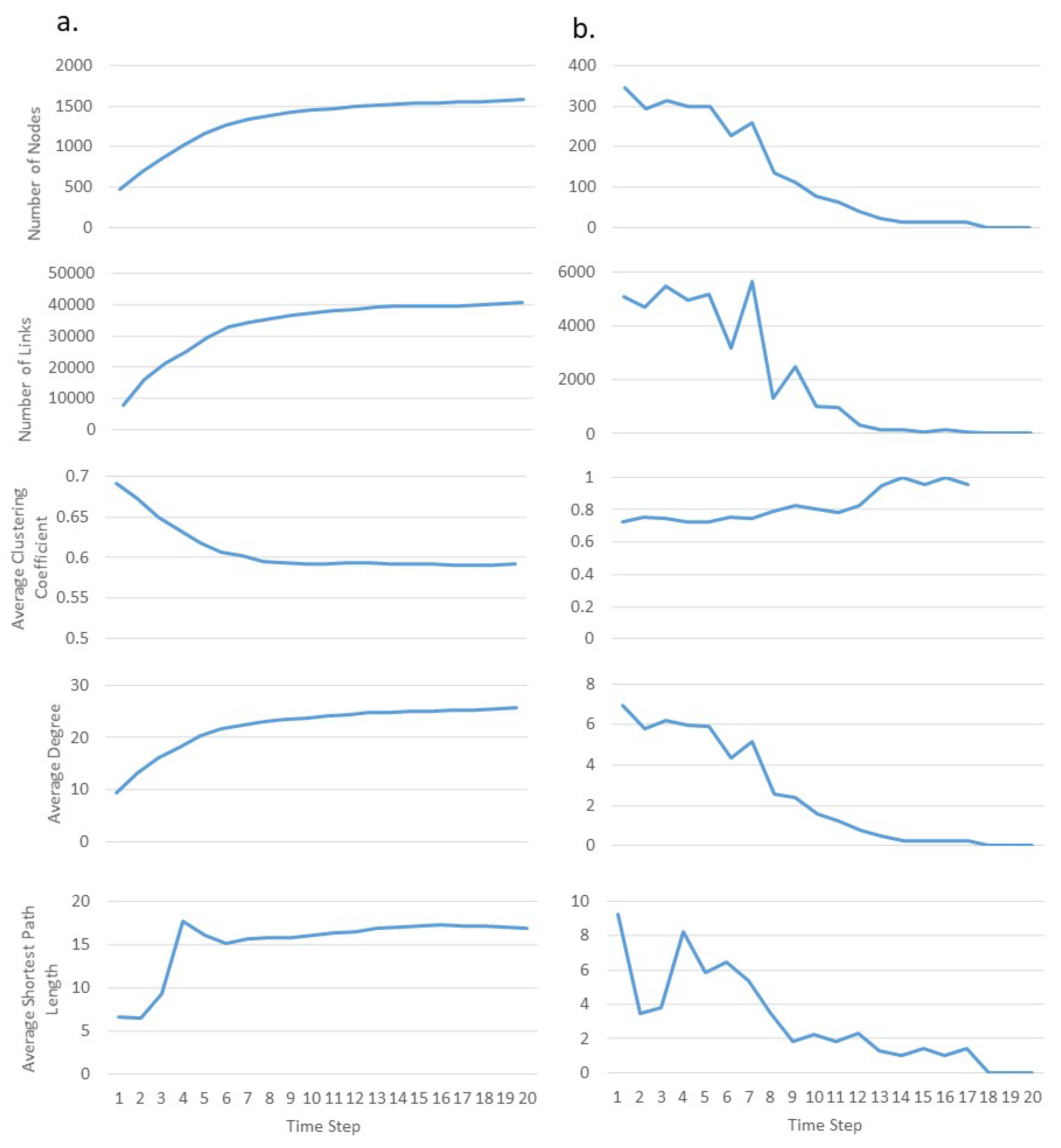
Figure 4.
Calculated degree distribution for each evolving spatial network SNGOL as it evolves over time generated from (a) scenario 1: network growth and (b) scenario 2: network shrinkage.
Figure 4.
Calculated degree distribution for each evolving spatial network SNGOL as it evolves over time generated from (a) scenario 1: network growth and (b) scenario 2: network shrinkage.

Figure 5.
Based on (a) the initial state, the evolving spatial network SNSEG generated from the GNASEG is presented as it becomes increasingly segregated at (b) t20. The inset maps for each time step are presented for each showing the composition of neighborhoods at t0 and t20, respectively.
Figure 5.
Based on (a) the initial state, the evolving spatial network SNSEG generated from the GNASEG is presented as it becomes increasingly segregated at (b) t20. The inset maps for each time step are presented for each showing the composition of neighborhoods at t0 and t20, respectively.

Figure 6.
Values obtained for number of nodes, number of links, average clustering coefficient, average degree, average path length, and assortativity for the spatial network SNSEG as it evolves over space and time.
Figure 6.
Values obtained for number of nodes, number of links, average clustering coefficient, average degree, average path length, and assortativity for the spatial network SNSEG as it evolves over space and time.
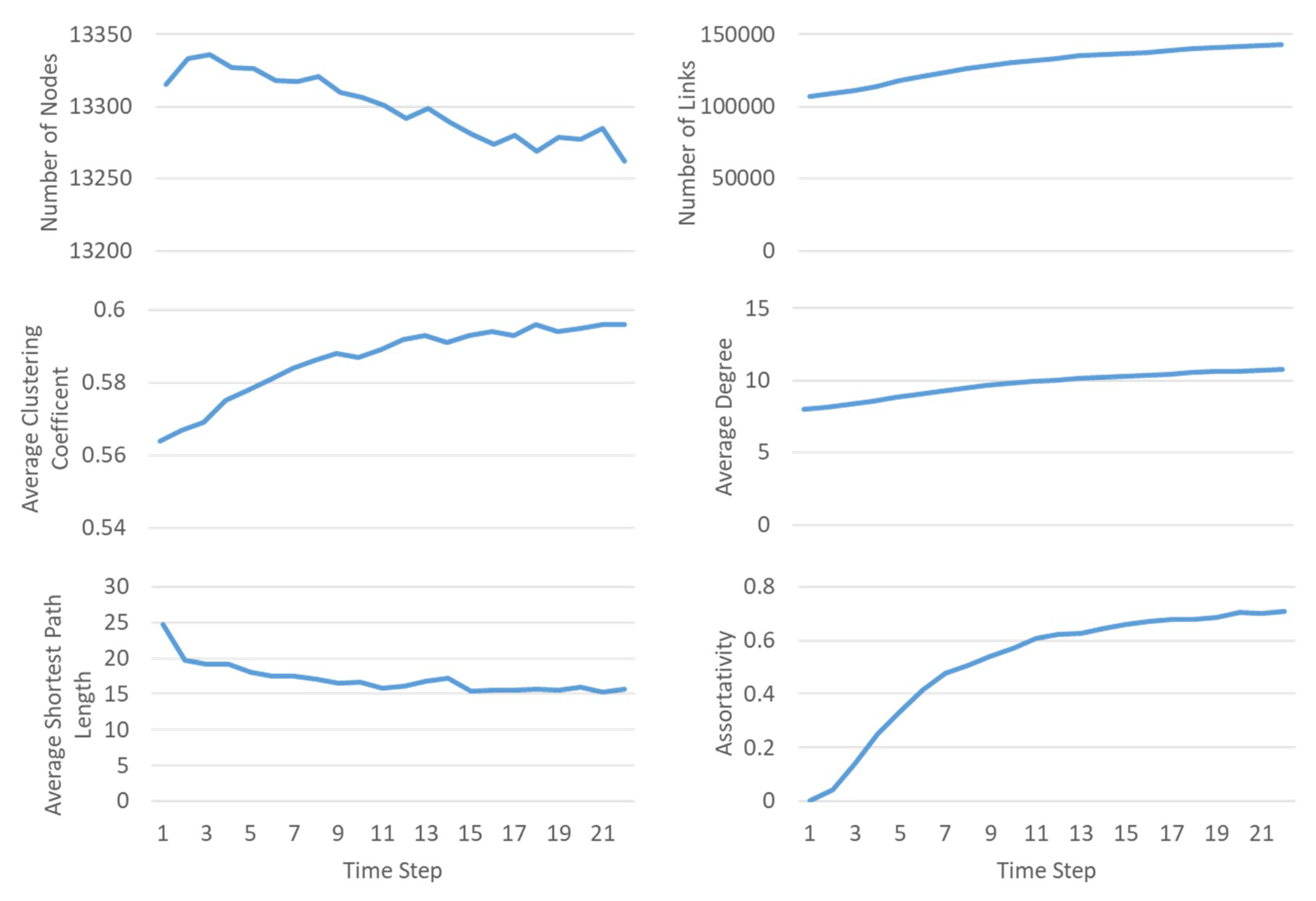
Figure 7.
Obtained degree distributions for each evolving spatial network SNSEG as it evolves over time.
Figure 7.
Obtained degree distributions for each evolving spatial network SNSEG as it evolves over time.


Table 1.
Operationalizing the GNA approach.
| Stage | Description |
|---|---|
| 1. Conceptualize system of interest as spatial network SN | Define • the components that make up the systems of interest to be represented as nodes • the interactions, flows, and relationships to be represented as links • the node and link spatial, non-spatial, and topological attributes Determine • whether the phenomenon is best represented by a weighted or directional network whether there is an underlying network UN structure that influences the spatial network SN and vice versa Consider the scale at which the system has been abstracted and the limitations |
| 2. Identify important graph theory measures | Identify which global or local graph theory measures are valuable to measure the spatial or non-spatial characteristics of the evolving spatial network SN. This is a function of the purpose of the model. |
| 3. Determine the neighborhood J | Determine which t nodes are within the neighborhood of node based on distance, weight, cost, and/or probability |
| 4. Develop transition rules | Develop the rules representing interactions between neighboring nodes that result in network evolution i.e., change of state, location, or connectivity of nodes |
| 5. Develop connection costs | Identify influences that the matrix has on network structure i.e., geographic barriers, distance thresholds, cost surface |
| 6. Implement the GNA | Input geospatial datasets to represent geographic barriers, cost surface analysis, underlying network UN structures, and/or initial spatial network SN Develop • georeferenced node automata and link objects based on conceptualization • programming functions that implement transition rules and connection costs • programming functions that calculate local and global graph theory measures |
| 7. Test the GNA | Perform sensitivity testing, model calibration, and validation using independent datasets |
| 8. Execute model and scenarios | Execute model and scenarios for the necessary number of time steps |
| 9. Apply graph theory to characterize network structures | Execute developed programming functions that calculate local and global graph theory measures to enhance the understanding of the phenomena being simulated, to compare network structures as the network evolves, or to compare network structures between scenarios |
Table 2.
Examples of spatial, non-spatial, and network properties for both nodes v and links e.
| Property Type | Description | Examples of Node Properties | Examples of Link Properties |
|---|---|---|---|
| Spatial | Geometric properties pertaining to the node v or link l | Location (x, y coordinates), area, distance from, perimeter | Length, coordinates of end points, direction |
| Non-Spatial | Qualitative and quantitative non-spatial attributes pertaining to the node v or link l | Name, ID, color, value, type, state | Name, ID, color, value, type, state |
| Network | Measurements derived from network theory pertaining to the node v or link l | Degree, betweenness, weight, clustering coefficient, list of neighbors | Weight, list of end nodes |
Table 3.
Selected graph theory measures to characterize and analyze spatial networks.
| Graph Theory Measure | Definition |
|---|---|
| Average degree <k> | The number of connections a node has to other nodes in the network is a localized measure, specific to each node, and is referred to as node degree k. Therefore, the mean degree across all nodes in the network is referred to as average degree <k>. |
| Degree distribution P(k) | The fraction of nodes in the network with degree k, calculated for the entire distribution of k is referred to as degree distribution P(k). |
| Average clustering coefficient <C> | Clustering coefficient C measures the likelihood of nodes that are connected to node i are also connected to each other. When C = 1, all nodes connected to node i are also connected to each other and when C = 0, none are connected to each other. This is a localized measure specific to each node. Average clustering coefficient <C> measures the average C across all nodes in the network. |
| Average shortest path length <l> | The average number of intermediate nodes and links in the shortest path between all pairs of nodes in the network is referred to as average path length <l>. |
Table 4.
Transition rules and their parameterization specific to each scenario for GNAGOL.
| Rule | Scenario | Parameter x |
|---|---|---|
| R1. To simulate the dynamics of underpopulation, any live node i with x live neighbors j dies and is removed from the spatial network SN | Scenario 1 | ≤6 |
| Scenario 2 | ≤11 | |
| R2. To simulate the dynamics of survival of the fittest, any live node i with x live neighbors j maintains their alive state and thus their place in the spatial network SN. | Scenario 1 | =7, 8, 13, or 14 |
| Scenario 2 | NA | |
| R3. To simulate the dynamics of overpopulation, any live node i with x live neighbors j dies and is removed from the spatial SN. | Scenario 1 | ≥15 |
| Scenario 2 | ≥20 | |
| R4. To simulate the dynamics of reproduction, any dead node with x live neighbors j becomes a live node and is added to the spatial network SN. | Scenario 1 | >8 and <13 |
| Scenario 2 | >11 and <20 |
Table 5.
Correlation matrix presenting the Pearson’s Correlation (r) for each pair of the graph theory measures obtained from the evolving spatial network SNGOL generated by two scenarios representing (a) network growth and (b) network shrinkage. Each graph theory measure is numbered from 1 to 5.
Table 5.
Correlation matrix presenting the Pearson’s Correlation (r) for each pair of the graph theory measures obtained from the evolving spatial network SNGOL generated by two scenarios representing (a) network growth and (b) network shrinkage. Each graph theory measure is numbered from 1 to 5.
| (a) Scenario 1: Network Growth | |||||
| Graph Theory Measure | (1) | (2) | (3) | (4) | (5) |
| (1) Number of Nodes | 1.00 | ||||
| (2) Number of Links | 0.99 | 1.00 | |||
| (3) Average Clustering Coefficient | −0.97 | −0.98 | 1.00 | ||
| (4) Average Path Length | 0.79 | 0.79 | −0.82 | 1.00 | |
| (5) Average Degree | 0.99 | 0.99 | −0.98 | 0.8 | 1.00 |
| (b) Scenario 2: Network Shrinkage | |||||
| Graph Theory Measure | (1) | (2) | (3) | (4) | (5) |
| (1) Number of Nodes | 1.00 | ||||
| (2) Number of Links | 0.94 | 1.00 | |||
| (3) Average Clustering Coefficient | −0.73 | −0.67 | 1.00 | ||
| (4) Average Path Length | 0.74 | 0.94 | −0.58 | 1.00 | |
| (5) Average Degree | 0.99 | 0.95 | −0.72 | 0.74 | 1.00 |
Table 6.
Correlation matrix presenting Pearson’s Correlation (r) for each pair of the graph theory measures obtained from the evolving spatial network SNSEG. Each graph theory measure is numbered from 1 to 5.
Table 6.
Correlation matrix presenting Pearson’s Correlation (r) for each pair of the graph theory measures obtained from the evolving spatial network SNSEG. Each graph theory measure is numbered from 1 to 5.
| Graph Theory Measures | (1) | (2) | (3) | (4) | (5) | (6) |
|---|---|---|---|---|---|---|
| (1) Number of Nodes | 1.00 | |||||
| (2) Number of Links | −0.82 | 1.00 | ||||
| (3) Average Clustering Coefficient | −0.72 | 0.97 | 1.00 | |||
| (4) Average Path Length | 0.42 | −0.74 | −0.80 | 1.00 | ||
| (5) Average Degree | −0.83 | 0.99 | 0.96 | −0.74 | 1.00 | |
| (6) Assortativity | −0.70 | 0.95 | 0.99 | −0.82 | 0.95 | 1.00 |
© 2020 by the authors. Licensee MDPI, Basel, Switzerland. This article is an open access article distributed under the terms and conditions of the Creative Commons Attribution (CC BY) license (http://creativecommons.org/licenses/by/4.0/).
Share and Cite
MDPI and ACS Style
Anderson, T.; Dragićević, S. Representing Complex Evolving Spatial Networks: Geographic Network Automata. ISPRS Int. J. Geo-Inf. 2020, 9, 270. https://0-doi-org.brum.beds.ac.uk/10.3390/ijgi9040270
AMA Style
Anderson T, Dragićević S. Representing Complex Evolving Spatial Networks: Geographic Network Automata. ISPRS International Journal of Geo-Information. 2020; 9(4):270. https://0-doi-org.brum.beds.ac.uk/10.3390/ijgi9040270
Chicago/Turabian StyleAnderson, Taylor, and Suzana Dragićević. 2020. "Representing Complex Evolving Spatial Networks: Geographic Network Automata" ISPRS International Journal of Geo-Information 9, no. 4: 270. https://0-doi-org.brum.beds.ac.uk/10.3390/ijgi9040270
Note that from the first issue of 2016, this journal uses article numbers instead of page numbers. See further details here.