Article

Comparing Machine Learning Models and Hybrid Geostatistical Methods Using Environmental and Soil Covariates for Soil pH Prediction

by
Panagiotis Tziachris
1,*,
Vassilis Aschonitis
1,
Theocharis Chatzistathis
1,
Maria Papadopoulou
2 and
Ioannis (John) D. Doukas
3
1
Soil and Water Resources Institute, Hellenic Agricultural Organization (H.A.O.)-DEMETER, 570 01 Thessaloniki, Greece
2
Department of Cadastre, Photogrammetry and Cartography, Faculty of Engineering, Aristotle University of Thessaloniki (AUTH), 541 24 Thessaloniki, Greece
3
School of Civil Engineering, Faculty of Engineering, Aristotle University of Thessaloniki (AUTH), 541 24 Thessaloniki, Greece
*
Author to whom correspondence should be addressed.
ISPRS Int. J. Geo-Inf. 2020, 9(4), 276; https://0-doi-org.brum.beds.ac.uk/10.3390/ijgi9040276
Submission received: 28 February 2020 / Revised: 29 March 2020 / Accepted: 16 April 2020 / Published: 23 April 2020

Abstract

:
In the current paper we assess different machine learning (ML) models and hybrid geostatistical methods in the prediction of soil pH using digital elevation model derivates (environmental covariates) and co-located soil parameters (soil covariates). The study was located in the area of Grevena, Greece, where 266 disturbed soil samples were collected from randomly selected locations and analyzed in the laboratory of the Soil and Water Resources Institute. The different models that were assessed were random forests (RF), random forests kriging (RFK), gradient boosting (GB), gradient boosting kriging (GBK), neural networks (NN), and neural networks kriging (NNK) and finally, multiple linear regression (MLR), ordinary kriging (OK), and regression kriging (RK) that although they are not ML models, they were used for comparison reasons. Both the GB and RF models presented the best results in the study, with NN a close second. The introduction of OK to the ML models’ residuals did not have a major impact. Classical geostatistical or hybrid geostatistical methods without ML (OK, MLR, and RK) exhibited worse prediction accuracy compared to the models that included ML. Furthermore, different implementations (methods and packages) of the same ML models were also assessed. Regarding RF and GB, the different implementations that were applied (ranger-ranger, randomForest-rf, xgboost-xgbTree, xgboost-xgbDART) led to similar results, whereas in NN, the differences between the implementations used (nnet-nnet and nnet-avNNet) were more distinct. Finally, ML models tuned through a random search optimization method were compared with the same ML models with their default values. The results showed that the predictions were improved by the optimization process only where the ML algorithms demanded a large number of hyperparameters that needed tuning and there was a significant difference between the default values and the optimized ones, like in the case of GB and NN, but not in RF. In general, the current study concluded that although RF and GB presented approximately the same prediction accuracy, RF had more consistent results, regardless of different packages, different hyperparameter selection methods, or even the inclusion of OK in the ML models’ residuals.

1. Introduction

Environmental sciences have always been interested in accurately predicting the spatial distributions of different phenomena regarding soil, water, air, etc. [1,2,3,4]. Currently, the increased numbers of digital data (Internet of Things, high-accuracy digital elevation models (DEM), satellite images) present a great opportunity for improved prediction results.
Initially, the prediction of spatial phenomena was achieved with the use of spatial prediction methods which mainly fell into the following two categories: deterministic methods, like inverse distance weighting or nearest neighbors, and stochastic ones, like regression models and kriging variations (e.g., ordinary kriging, universal kriging, etc.). Later on, hybrid methods were introduced [5,6,7] that were partially deterministic, partially stochastic, like regression kriging (RK) or kriging with external drift (KED). These methods tried to combine the advantages of both worlds, deterministic and stochastic, achieving improved results. Currently, more innovative implementations of the abovementioned hybrid methods are increasingly used; they introduce machine learning (ML) as the deterministic part, along with kriging of the ML residuals as the stochastic part [8,9,10,11,12]. These methods are widely used in environmental sciences mainly for two reasons: their improved prediction accuracy and the elimination of most of the restrictions (e.g., statistical assumptions) that regression, kriging, and their variations (RK, KED, etc.) demand [9,13].
Usually, scientists, in their environmental studies, assess multiple ML models so as to find the one that maximizes the prediction accuracy for a specific phenomenon [14,15,16,17]. They use specific ML implementations (packages, methods) and try to estimate the best hyperparameters for their models that produce the most accurate results. However, it is not obvious as to whether the different ML implementations of the same ML model and the different hyperparameter selection methods significantly affect the results.
Soil pH is a crucial soil parameter that affects both the soil properties and the plants themselves. It greatly influences the behavior of chemical elements and, along with organic matter (OM), is the most important parameter determining trace metal partitioning and aqueous speciation in soils [18]. It is considered of special importance in connection with nutrients [19] and micronutrients [20], and it is the key variable that affects plant growth [21]. It controls soil fertility, regulates soil biogeochemical processes, and influences the structure and functioning of terrestrial ecosystems [22]. Regarding its spatial distribution, soil pH seems to be affected by terrain elevation [23] and exhibits spatial cross correlation with other elements, like soil Fe [24]. Based on the above characteristics, soil pH was considered the ideal soil parameter for the current study.
The aim of the present study is manifold. Firstly, we compare the predictive capabilities of the different ML and non-ML models, with and without kriging of their residuals, in soil pH prediction. The ML models that are assessed are random forests (RF), random forests kriging (RFK), gradient boosting (GB), gradient boosting kriging (GBK), neural networks (NN), and neural networks kriging (NNK),along with the non-ML models of multiple linear regression (MLR), ordinary kriging (OK), and regression kriging (RK) as traditional/hybrid geostatistical methods. Secondly, the effects of the different implementations (methods and packages in R) of the same ML models are also evaluated. For the RF model, the ranger and rf methods are used; for GB, xgbTree and xgbDART; and for NN, nnet and avNNet. Finally, the last goal is to investigate whether the selection methods of the hyperparameters (default vs. optimized through random search) affect the results of the different ML models.

2. Materials and Methods

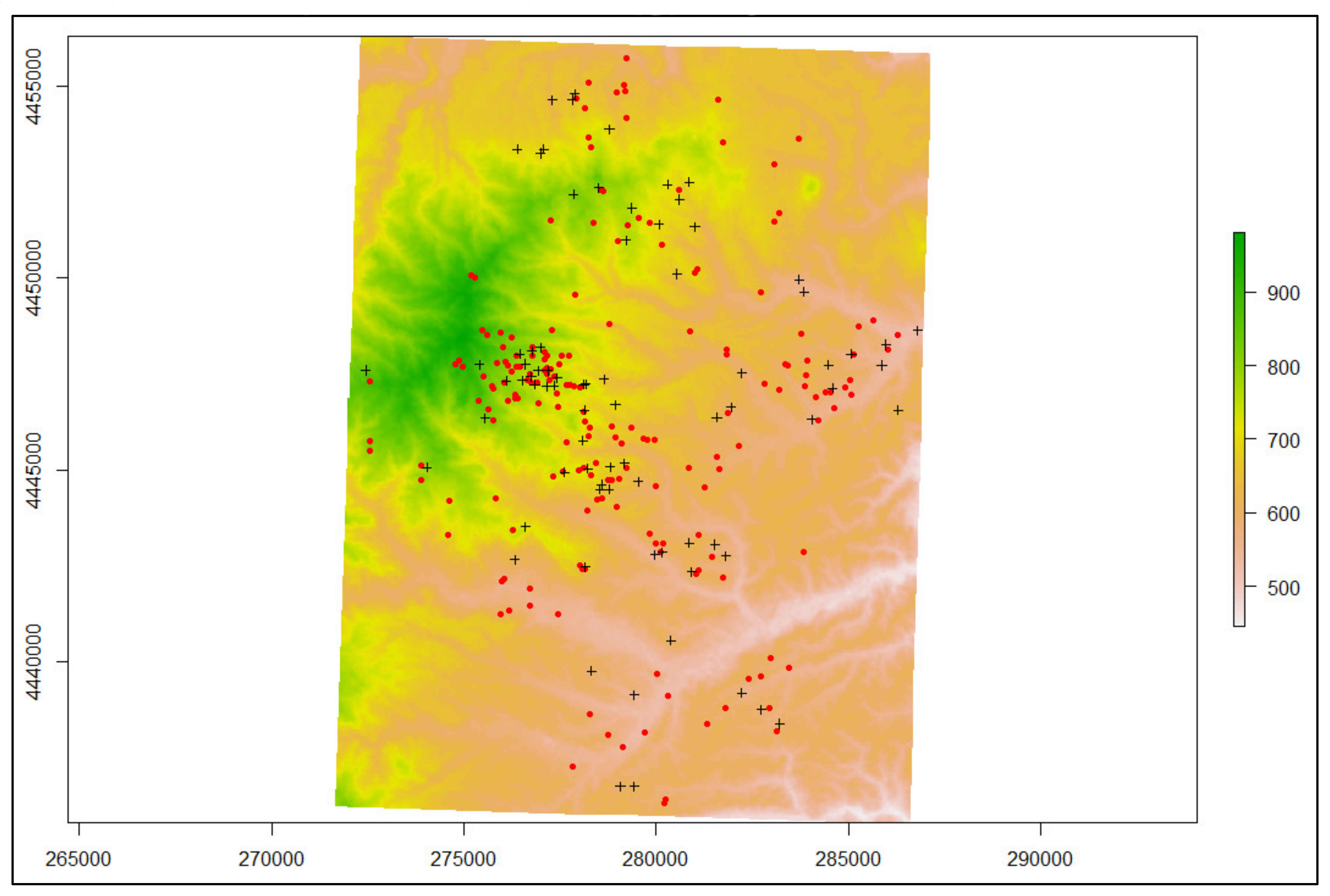
2.1. Soil Data and Environmental Covariates Collection

The study area (Figure 1) is located in the regional unit of Grevena in northern Greece, and it extends from latitude 40°01′50.76″ N to 40°14′43.79″ N and from longitude 21°17′30.06″ E to 21°33′25.43″ E in the World Geodetic System of 1984 (WGS84). The altitude ranges from approximately 500 m above sea level up to 900 m further north, and the area covers approximately 270 km2.
A soil survey was conducted for three years (2015, 2017, and 2018), mainly around autumn and early winter of each year. Specifically, 266 disturbed soil samples were obtained from randomly selected locations using a simple random sampling design (Soil Survey Division Staff, 2017) with a soil auger from depth 0–30 cm of the surface soil. At each location, representative samples were taken (2–3) close to each other and pooled together to make a composite sample. Global Positioning System (GPS) receivers were utilized to identify the sampling positions. The minimum distances between two sampling points range around 50 m, and the average distance between points is 300 m.
In this study, soil covariates and environmental covariates were used (Table 1). Regarding soil covariates, the 266 soil samples that were collected from the Grevena area were analyzed in the laboratory of the Soil and Water Resources Institute for clay (C), silt (Si), sand (S), electric conductivity (EC), organic matter (OM), nitrogen (N), phosphorus (P), potassium (K), magnesium (Mg), iron (Fe), zinc (Zn), manganese (Mn), copper (Cu), and boron (B). Moreover, pH analysis for the same locations was conducted to calibrate the models and to assess the prediction results.
The environmental covariates were derived from the second version of the Aster Global Digital Elevation Model (GDEM2) using SAGA-GIS software modules. Aster consists of 1° × 1° tiles (30 m resolution) in the World Geodetic System 1984 (WGS84), reprojected to the Greek Geodetic Reference System 1987 (GGRS87) for this study (Figure 2).

2.2. Software

The statistical analysis was implemented using statistical software R (version 3.5.3) and the caret package [25]. In the current study, different packages and methods were utilized in R through caret: a) xgboost along with the xgbTree methods from the xgboost package for GB, b) the randomForest and ranger packages for RF, and c) the avNNet and nnet methods from the nnet package for NN. The geostatistics in the current paper were implemented using the gstat package. Finally, SAGA-GIS software (http://www.saga-gis.org/en/index.html) was used to produce the different terrain attributes.

2.3. Regression Kriging

Regression kriging is a hybrid geostatistical method that combines multiple linear regression between the target soil variable and secondary parameters with geostatistical methods (e.g., ordinary kriging or simple kriging) on the residuals of the regression. Its goal is to optimize the prediction of soil properties in unsampled locations [26] based on the assumption that the deterministic component of the target soil variable is accounted for by the regression model, while the model residuals represent the spatially varying but dependent component [7].
Specifically, in the case of multiple linear regression and ordinary kriging, the prediction Z ^ R K s i for s i locations is the sum of the prediction of the regression Z ^ R s i for the same locations and the prediction of the kriged residuals of the regression ε ^ O Κ , as seen in the following equation.
Z ^ R K s i = Z ^ R s i + ε ^ O Κ
In this equation there are two distinct parts. The first one, Z ^ R s i ,   is the deterministic component, and the second one, ε ^ O Κ , is the stochastic. These two distinct parts allow for separate interpretation of the two components and the application of different regression techniques [6].

2.4. Random Forests Kriging

Random forest [27,28] is a machine learning model based on classification and regression trees [29] that provides increased prediction accuracy. In RF, a large collection of de-correlated, noisy, approximately unbiased trees are built and averaged so as to reduce model variance and cope with instability [30]. This is achieved by growing multiple trees combining twofold randomness: random selection of examples in the training dataset and random features used from the same dataset. As in every machine learning model, there are parameters that can be optimized; in the case of the ranger/randomForest packages, there are mainly two: mtry and ntree (Table 2).
Even though there might be more hyperparameters depending on the RF packages that are utilized, these two presented here are the most commonly used. The packages utilized in the current study were ranger [31] and randomForest [32].
Finally, OK was applied to the RF residuals ( ε ^ O K ) and then added to the RF prediction results Z ^ R F s i at the s i locations so as to estimate RFK according to Equation (2):
Z ^ R F K s i = Z ^ R F s i + ε ^ O K .
This resembles Equation (1); however, the deterministic component Z ^ R F s i   uses random forests instead of regression.

2.5. Gradient Boosting Kriging

In gradient boosting [33], multiple decision trees are grown sequentially using information from previously grown existing trees. Even though each tree is small and with few terminal nodes, they manage to boost the overall performance by addressing problematic observations with large errors. That way, they improve the model in areas where it does not perform well, resulting in a more accurate prediction model. Specifically in the case of gradient boosting, each tree is fitted to the residuals of the previous model using a gradient descent algorithm that minimize a loss function associated with the whole ensemble.
There are multiple packages that can perform GB (CatBoost, LightGBM, XGBoost, etc.), with different implementations and different results. In the current study, “eXtreme Gradient Boosting” from the XGBoost [34] package was utilized through caret by implementing two different methods: XgbDART and xgbTree. The eXtreme Gradient Boosting is considered an efficient and scalable implementation of the gradient boosting framework in which a more regularized model formalization is used to control overfitting and achieve better performance. Some of its advantages are the following:
  • A regularization technique that helps reducing overfitting;
  • Support for user-defined objective functions and evaluation metrics;
  • Improved efficient tree pruning mechanism;
  • Multiple technical improvements like parallel processing, “built-in cross-validation”, and better handling of missing values.
There are multiple parameters that need to be tuned in this model (Table 3), and they can be classified into a) the general parameters that control the booster type, b) the linear booster parameters that control the performance of the linear booster, and c) the learning task parameters that specify the learning task and the corresponding learning objective.
The introduction of kriging as the stochastic part (GBK) is calculated based on the following equation:
Z ^ G B K s i = Z ^ G B s i + ε ^ O K .
The OK method is performed on the residuals of the GB ( ε ^ O K ) , and the OK results are added to the GB predictions Z ^ G B s i .

2.6. Neural Networks Kriging

Neural networks (or artificial neural networks) are powerful tools, modeled loosely after the human brain, that use a machine learning approach to quantify and model complex behavior and patterns. They perform tasks by considering examples, generally without being programmed with task-specific rules. A NN consists of a set of interconnected units called neurons, which estimate the nonlinear correlations between each variable. The input neurons, which represent predictor variables, are connected to a single or multiple layer(s) of hidden neurons, which are then linked to the output neurons that represent the target soil variable [35].
For the NN in the current study, the nnet package was used with two different methods: nnet and avNNet. The nnet package [36,37] is software for feed-forward neural networks with a single hidden layer, and for multinomial log-linear models. In a feed-forward NN, the information moves in only one direction (forward); from the input nodes, through the hidden nodes, and to the output nodes. The nnet method implements exactly this model to predict the results.
The avNNet method of the nnet package aggregates several feed-forward neural network models by fitting different random numbers of seeds. In the case of regression, like that used in the current study, all the resulting models were used for prediction by averaging the results coming from each network.
The exact hyperparameters of the NN that were tuned in the current study, along with their descriptions, are presented in Table 4. Most of them were used in both methods, apart from bag, which was used only in avNNet.
Finally, the neural networks kriging (NNK) is based on the following equation:
Z ^ N N K s i = Z ^ N N s i + ε ^ O K .
The residuals ε ^ O K   are used for OK, and the prediction results are added to the NN prediction.

2.7. Optimization of the Hyperparameters

Every ML model needs to have its hyperparameters defined before training. This could be achieved by using the following:
  • Default values based on the literature, library authors’ recommendations, previous experience, etc.;
  • Optimizations techniques, through a process called tuning.
Tuning can be implemented in multiple ways, like grid search, random search, Sobol sequence, manual, and others. Grid search and random search are the most commonly applied. In grid search, every combination from a preset list of values of the hyperparameters is estimated and used to evaluate the model for each combination. In the current study, however, random search was performed, in which random combinations of parameters were employed from a range of values. Random search was preferred here due to the improved results that it provides according to the literature [38]. The model with the set of parameters which gave the highest accuracy was considered to be the best and was used for prediction.
Random search was implemented through the caret package. It is important to state here that in general, the hyperparameters that can be optimized through caret are usually fewer than the actual parameters that the package can support by itself. However, they are usually the most important ones that significantly affect the results of each model. Along with random search, the same ML models were trained with default values, and the results were compared.

2.8. Error Assessment

The 266 samples of the current study were randomly split into two datasets: the training dataset (80% of the data) that was used for estimating the models, and the testing dataset (20% of the data) that was used for assessing the different models. The optimization of the models’ parameters was implemented using 10-fold cross-validation techniques in the training dataset.
Different metrics (Table 5) were employed to estimate model performance based on the difference between the observations and the predictions on the testing data set. The root-mean-square error (RMSE) and the mean absolute error (MAE) were estimated based on the measured value Z s i and its prediction Z ^ s i for the locations s i of the samples. Lower values of RMSE and MAE are associated with better predictive results. Also, the coefficient of determination (R2), which represents the amount of variation explained by the model, was estimated. The terms SSE and SSTO represent the error sum of squares and the total sum of squares, respectively. The coefficient of determination ranges from 0 to 1, where for 0 (zero), no variation is explained by the model, and for 1 (one), all variation is explained by the model.

3. Results

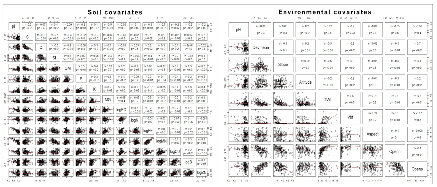
3.1. Exploratory Data Analysis

The soil co-variables that were measured in the laboratory were clay (C), silt (Si), sand (S), electrical conductivity (EC), organic matter (OM), nitrogen (N), phosphorus (P), potassium (K), magnesium (Mg), iron (Fe), zinc (Zn), manganese (Mn), copper (Cu), boron (B), and pH from the 266 locations in the Grevena area (Table 6). Some of them, those that significantly deviated from normality and strongly affected the residuals of MLR, were log transformed (EC, N, Fe, Mn, Cu, B, and Zn). The rest remained untransformed because they did not significantly affect the normality assumption of the MLR residuals.
Based on the Pearson correlation analysis for pH (Figure 3), there was a statistically significantly strong correlation with logFe ( p 0.01 ,   r = 0.8 ) and logMn p 0.01 ,   r = 0.7 and moderate correlation with Mg and Si. In general, the soil covariates exhibited stronger correlation with the pH than did the environmental ones.

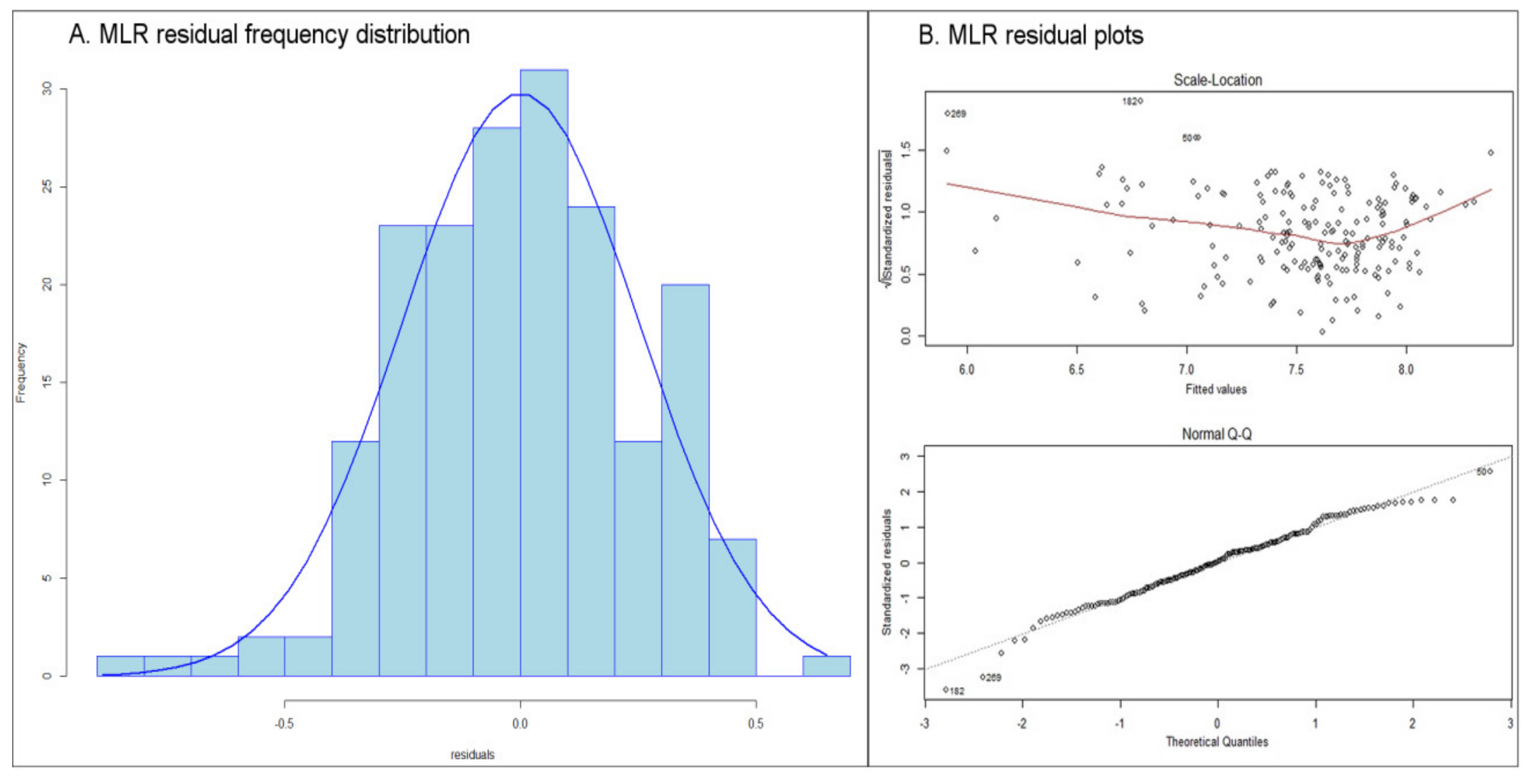
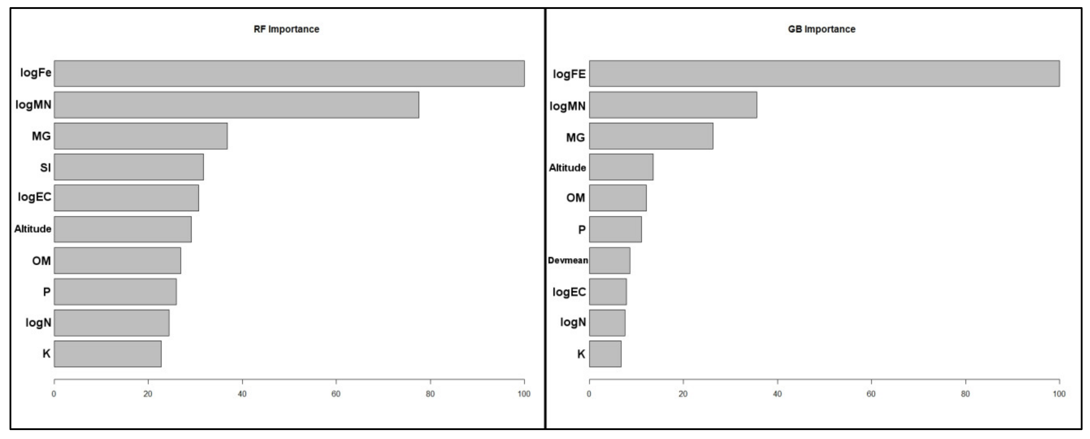
3.2. Modelling and Parameter Estimation

Regression kriging was conducted on the training data set by combining multiple linear regression between the target soil variable and the secondary parameters with ordinary kriging on the residuals of the regression (Eq. 1).
A stepwise procedure was utilized to select the best regression predictors, which in our study were C, OM, P, K, Mg, Devmean, Altitude, Aspect, logEC, logN, logFe, logMn, and logZn. The final regression equation was:
Y p H = 9.477 + 0.007547 C + 0.1284 O M 0.008084 P + 0.0004580 K 0.0003164 M g + 0.1321 log E C 0.1287 log N 0.2764 log F e 0.4176 log M n 0.6231 log Z n 0.06426 D e v m e a n 0.0004279 A l t i t u d e 0.01974 A s p e c t .
The residuals of the regression presented a distribution close to normal, as seen in the residual frequency distribution diagram (Figure 4A) and normal Q–Q plot (Figure 4B, bottom), having approximately constant standard deviation errors (homoscedasticity) (Figure 4B, top). Also, the Shapiro–Wilk statistic (W) for the residuals was computed (W = 0.98588, p-value = 0.05638). Based on the results, for the significance level of 0.05, we cannot reject the hypothesis that the residuals come from a population which has a normal distribution.
For random forests, a 10-fold cross-validation method on the training data set was applied to pick the optimal hyperparameter values via the random search tuning process (Table 7). The default mtry value was estimated at close to one-third of the total number of variables used in RF [30], which in this case was 8.
The number of grown trees (num.trees in ranger and ntree in randomForest) could not be tuned through caret, so the default value of the packages was used (500) for both of them. Hyphens (empty cells) in Table 7, Table 8, and Table 9 were used to signify the lack of a hyperparameter for the specific method. For the estimation of RFK for each package, the residuals of RF were used for OK interpolation, and the results were added to the RF according to Equation (2).
Gradient boosting has a plethora of hyperparameters that need to be defined (Table 8). For the default values, the libraries’ default parameters were chosen. In the case of optimized values, the random search tuning process was used with 10-fold cross-validation of the training data. At the end, the residuals of the GB were used for OK and the results were added (Equation (3)) in order to estimate the GBK for each method.
Finally, regarding NN, the hyperparameters that were used are presented in Table 9. The default values were the ones that the library proposed. For the optimized hyperparameters, “size” and “decay” were tuned through a random search tuning process with 10-fold cross-validation.
Similar to the previous ML models, the residuals of NN were used for OK, and the results were added (Equation (4)) in order to estimate the NNK.

3.3. Performance Assessment

The models in the current study were assessed based on the difference between the pH observations and their predictions. According to the prediction results, machine learning algorithms (RF, GB, NN) exhibited better accuracy in every metric when compared to the MLR, RK, or OK (Table 10). For example, RK (the best of the non-ML models) presented higher RMSE than almost all the ML algorithms, apart from NNnnD (NN with its default values). In more detail, RK’s RMSE (0.336) was 14% higher compared to the mean of all the ML RMSE values (0.289), and RK’s R2 (0.626) was 15% lower than the mean R2 of all ML models (0.723). Comparing the best implementation of each ML model, RK exhibited a 23% decrease in RMSE and 25% increase in R2 in the case of RFrgO (RMSE of 0.259, R2 of 0.781), a 22% decrease in RMSE and 24% increase in R2 in the case of GBKxgbT (RMSE of 0.262, R2 of 0.778), and finally, a 20% decrease in RMSE and 21% increase in R2 in the case of NNnnO (RMSE of 0.268, R2 of 0.760). The results were even worse for the OK. This was expected though, since OK does not incorporate the information of multiple covariates that the other methods do.
Among the ML models, RF exhibited high prediction accuracy, with the RFrfO model being the best one with small RMSE (0.259), high R2 (0.784), and low MAE (0.180). GB was very close, with GBKxgbT (RMSE:0.262, R2: 0.778, MAE:0.177) presenting the best results among the GB models. NN performed slightly worse, with NNnnO being the best NN model, scoring 0.268 in RMSE and 0.760 in R2; this was not too far from the other ML models, as can also be seen in Figure 5.
Optimization of the hyperparameters improved the prediction accuracy in the GB and NN models. Especially in the case of NN, the default values led to very poor quality models, as seen from NNnnD, which had the worst prediction results (RMSE of 0.468, R2 of 0.278, MAE of 0.312), and NNavD (RMSE of 0.353, R2 of 0.618, MAE of 0.261), the second worst among all ML models. In the case of RF, there were only a few hyperparameters involved in the optimization, and the default values were close to the optimized ones; therefore, the results were not really affected. The default values were based on suggestions from the literature and the libraries’ default values, which in our case were mtry = 8 and ntree = 500, almost the same as the optimization values (mtry = 9 and ntree = 500). Consequently, there were only minor differences in the models’ results between the default and optimized hyperparameters.
Kriging interpolation of the residuals did not significantly affect the results. It slightly improved NN and RK, whereas for RF, the results were slightly worsened. In more detail, in the case of GB, kriging of the residuals, as seen in GBKxgbT, improved the RMSE by approximately 6% and R2 by 3.8% compared to GBxgbTO, while GBKxgbD’s RMSE was improved by 4% and R2 by 2.4% compared to GBxgbDO. Regarding RF, the kriging of the residuals led to a minor increase in RFrgO’s RMSE by 1.7% and decrease in R2 by 0.2% as seen in RFKrg. Similarly there was a slight increase in RFrfO’s RMSE by 1.7% and decrease in R2 by 0.4% (RFKrf). For NN, the introduction of OK to the residuals led to a decrease in NNavO’s RMSE by 8% and an increase in R2 by 7.5% compared to NNKav, while the use of the nnet package (NNnnO) in NN led to similar results with a small increase in RMSE (1.3%) and decrease in R2 (0.7%), as seen in NNKnn. For RK, there was also an improvement with the introduction of OK to the residuals by 2.5% in RMSE and 3% in R2.
The use of different implementations (packages/methods) of the same ML models did not lead to major differences in the prediction results for RF and GB. In the case of RF, the results of RFrgO and RFrfO were similar, while in the case of GB (GBxgbTO and GBxgbDO), there were minor differences, with GBxgbTO being marginally better (RMSE of 0.279, R2 of 0.750, MAE of 0.190). In NN, the differences between the two methods (NNnnO and NNavO) were slightly larger.
It is worth mentioning that there were differences in the variability of the results between the different ML models. Specifically, RF results had the smallest variability (RMSE SD = 0.002, R2 SD = 0.002) compared to GB (RMSE SD = 0.32, R2 SD = 0.017) and NN (RMSE SD = 0.189, R2 SD = 0.078), regardless of the different packages that were utilized, the selection method of the hyperparameters, or the inclusion (or not) of OK of the residuals.
Regarding R2 in general, the values were high (Figure 5), over 0.6, especially for the ML models, apart from NNnnD. Therefore, the models explained most of the total variation of the pH, and the covariates used seem to strongly affect the soil pH. The MAE consistently had very low values in RF models, ranging from 0.178 up to 0.184. The GB results were close, but with higher variability (0.177 up to 0.232), and NN scored worse, with higher values ranging from 0.182 up to 0.312.
The covariate importance assessments (Figure 6) revealed that iron (Fe), manganese (Mn), and magnesium (Mg) were the most influential variables for both RF and GB. For iron (Fe) specifically, high influence on soil pH was expected according to the relevant literature [18,24]. Among the environmental variables, altitude was the one with the higher score for both ML models.

4. Discussion and Conclusions

From the results of the current study, it is obvious that ML models outperformed the other methods in predicting soil pH, like MLR or models that use kriging (RK or OK). Additionally, the ML models were easy to use, without the statistical assumptions and requisites that linear regression and kriging interpolation require. However, ML models demand significant computing power, along with knowledge and attention to the tuning process of the models. Overall, based on the results, the authors of the current study tend to agree with the claim that “…kriging as a spatial prediction technique might be redundant, but solid knowledge of geostatistics and statistics in general is important more than ever” [13].
The assessment of the prediction results of the different ML models shows that GB and RF have the best performance, with NN being slightly less accurate. The NN’s lesser results could be due to the fact that NN demands a big number of data in order to produce good predictions, e.g., 10 to 100 times the number of features or 10 times the number of inputs [39,40]. The 266 different locations and the 23 variables might not be enough for NN to show its predictive capabilities. Also, different implementations of the same ML model did not lead to major differences for RF and GB, whereas in NN, the differences were slightly bigger. Different implementations of the same ML models mainly introduce minor variations of the same ML models that might produce better results but only in some cases.
Optimization of the hyperparameters improved the prediction results in the GB and NN models due to the increased number of parameters and the significant difference between the default values and the optimized ones. It is obvious that their careful and thorough fine tuning is a crucial step for achieving the best results. In the case of RF, the hyperparameters were few and the default values were close to the optimized ones, leading to a minor difference in the prediction results.
The introduction of kriging interpolation of the ML models’ residuals did not really improve the results. This is in accordance with the findings by Henglet al. [41], stating that “…as a rule of thumb where once a machine learning model explains over 60% of variation in data, chances are that kriging is not worth the computational effort”.
The differences in the variability of the ML prediction results were expected based on the above-mentioned findings. In general, RF exhibited more consistent results with smaller variability, regardless of different packages or methods, different hyperparameter selection methods, or even the inclusion of kriging to the ML model residuals. This could be considered as an advantage in some cases where consistency is a requirement. The increased variability of the prediction results of the other ML models, however, suggests that they have the potential to further improve their prediction accuracy, for example, through a different tuning process or the use of different packages and implementations.

Author Contributions

Conceptualization, Panagiotis Tziachris; Data curation, Panagiotis Tziachris; Formal analysis, Vassilis Aschonitis; Investigation, Theocharis Chatzistathis; Methodology, Panagiotis Tziachris; Resources, Vassilis Aschonitis; Software, Panagiotis Tziachris; Validation, Maria Papadopoulou and Ioannis (John) D. Doukas; Writing—original draft, Panagiotis Tziachris; Writing—review and editing, Panagiotis Tziachris, Theocharis Chatzistathis, Maria Papadopoulou and Ioannis (John) D. Doukas. All authors have read and agreed to the published version of the manuscript.

Funding

This research received no external funding.

Acknowledgments

The authors would like to thank the chemists Tzeni Psoma, Areti Bountla, and the rest of the laboratory personnel of the Soil and Water Research Institute for their valuable help with the laboratory work.

Conflicts of Interest

The authors declare no conflict of interest.

References

  1. Appelhans, T.; Mwangomo, E.; Hardy, D.R.; Hemp, A.; Nauss, T. Evaluating machine learning approaches for the interpolation of monthly air temperature at Mt. Kilimanjaro, Tanzania. Spat. Stat. 2015, 14, 91–113. [Google Scholar] [CrossRef] [Green Version]
  2. Baxter, S.; Oliver, M. The spatial prediction of soil mineral N and potentially available N using elevation. Geoderma 2005, 128, 325–339. [Google Scholar] [CrossRef]
  3. Florinsky, I.V.; Eilers, R.G.; Manning, G.; Fuller, L. Prediction of soil properties by digital terrain modelling. Environ. Model. Softw. 2002, 17, 295–311. [Google Scholar] [CrossRef]
  4. Rahmati, O.; Pourghasemi, H.R.; Melesse, A.M. Application of GIS-based data driven random forest and maximum entropy models for groundwater potential mapping: A case study at Mehran Region, Iran. Catena 2016, 137, 360–372. [Google Scholar] [CrossRef]
  5. Bishop, T.; McBratney, A. A comparison of prediction methods for the creation of field-extent soil property maps. Geoderma 2001, 103, 149–160. [Google Scholar] [CrossRef]
  6. Hengl, T. A Practical Guide to Geostatistical Mapping of Environmental Variables; Office for Official Publications of the European Communities: Luxembourg, 2007. [Google Scholar]
  7. McBratney, A.B.; Odeh, I.O.; Bishop, T.F.; Dunbar, M.S.; Shatar, T.M. An overview of pedometric techniques for use in soil survey. Geoderma 2000, 97, 293–327. [Google Scholar] [CrossRef]
  8. Hengl, T.; de Jesus, J.M.; Heuvelink, G.B.; Gonzalez, M.R.; Kilibarda, M.; Blagotić, A.; Shangguan, W.; Wright, M.N.; Geng, X.; Bauer-Marschallinger, B. SoilGrids250m: Global gridded soil information based on machine learning. PLoS ONE 2017, 12, e0169748. [Google Scholar] [CrossRef] [PubMed] [Green Version]
  9. Keskin, H.; Grunwald, S. Regression kriging as a workhorse in the digital soil mapper’s toolbox. Geoderma 2018, 326, 22–41. [Google Scholar] [CrossRef]
  10. Mirzaee, S.; Ghorbani-Dashtaki, S.; Mohammadi, J.; Asadi, H.; Asadzadeh, F. Spatial variability of soil organic matter using remote sensing data. Catena 2016, 145, 118–127. [Google Scholar] [CrossRef]
  11. Song, Y.-Q.; Yang, L.-A.; Li, B.; Hu, Y.-M.; Wang, A.-L.; Zhou, W.; Cui, X.-S.; Liu, Y.-L. Spatial Prediction of Soil Organic Matter Using a Hybrid Geostatistical Model of an Extreme Learning Machine and Ordinary Kriging. Sustainability 2017, 9, 754. [Google Scholar] [CrossRef] [Green Version]
  12. Tziachris, P.; Aschonitis, V.; Chatzistathis, T.; Papadopoulou, M. Assessment of spatial hybrid methods for predicting soil organic matter using DEM derivatives and soil parameters. Catena 2019, 174, 206–216. [Google Scholar] [CrossRef]
  13. Hengl, T.; Nussbaum, M.; Wright, M.N.; Heuvelink, G.B.M.; Gräler, B. Random forest as a generic framework for predictive modeling of spatial and spatio-temporal variables. PeerJ 2018, 6, e5518. [Google Scholar] [CrossRef] [PubMed] [Green Version]
  14. Brillante, L.; Gaiotti, F.; Lovat, L.; Vincenzi, S.; Giacosa, S.; Torchio, F.; Segade, S.R.; Rolle, L.; Tomasi, D. Investigating the use of gradient boosting machine, random forest and their ensemble to predict skin flavonoid content from berry physical–mechanical characteristics in wine grapes. Comput. Electron. Agric. 2015, 117, 186–193. [Google Scholar] [CrossRef]
  15. Ransom, C.J.; Kitchen, N.R.; Camberato, J.J.; Carter, P.R.; Ferguson, R.B.; Fernández, F.G.; Franzen, D.W.; Laboski, C.A.M.; Myers, D.B.; Nafziger, E.D.; et al. Statistical and machine learning methods evaluated for incorporating soil and weather into corn nitrogen recommendations. Comput. Electron. Agric. 2019, 164, 104872. [Google Scholar] [CrossRef] [Green Version]
  16. Shirzadi, A.; Shahabi, H.; Chapi, K.; Bui, D.T.; Pham, B.T.; Shahedi, K.; Ahmad, B.B. A comparative study between popular statistical and machine learning methods for simulating volume of landslides. Catena 2017, 157, 213–226. [Google Scholar] [CrossRef]
  17. Sirsat, M.S.; Cernadas, E.; Fernández-Delgado, M.; Barro, S. Automatic prediction of village-wise soil fertility for several nutrients in India using a wide range of regression methods. Comput. Electron. Agric. 2018, 154, 120–133. [Google Scholar] [CrossRef]
  18. Kabata-Pendias, A. Trace Elements in Soils and Plants, 4th ed.; CRC Press: Boca Raton, FL, USA, 2010. [Google Scholar]
  19. Zhang, Y.; Biswas, A.; Adamchuk, V.I. Implementation of a sigmoid depth function to describe change of soil pH with depth. Geoderma 2017, 289, 1–10. [Google Scholar] [CrossRef]
  20. Sillanpää, M. Micronutrients and the Nutrient Status of Soils: A Global Study; Food & Agriculture Organization of the United Nations: Jokioinen, Finland, 1982. [Google Scholar]
  21. Gentili, R.; Ambrosini, R.; Montagnani, C.; Caronni, S.; Citterio, S. Effect of soil pH on the growth, reproductive investment and pollen allergenicity of Ambrosia artemisiifolia L. Front. Plant Sci. 2018, 9, 1335. [Google Scholar] [CrossRef] [Green Version]
  22. Hong, S.; Gan, P.; Chen, A. Environmental controls on soil pH in planted forest and its response to nitrogen deposition. Environ. Res. 2019, 172, 159–165. [Google Scholar] [CrossRef]
  23. He, X.; Hou, E.; Liu, Y.; Wen, D. Altitudinal patterns and controls of plant and soil nutrient concentrations and stoichiometry in subtropical China. Sci. Rep. 2016, 6, 24261. [Google Scholar] [CrossRef] [Green Version]
  24. Tziachris, P.; Metaxa, E.; Papadopoulos, F.; Papadopoulou, M. Spatial Modelling and Prediction Assessment of Soil Iron Using Kriging Interpolation with pH as Auxiliary Information. ISPRS Int. J. Geo-Inf. 2017, 6, 283. [Google Scholar] [CrossRef] [Green Version]
  25. Kuhn, M. The Caret Package. Available online: http://topepo.github.io/caret/index.html (accessed on 20 January 2020).
  26. Hengl, T.; Heuvelink, G.B.; Rossiter, D.G. About regression-kriging: From equations to case studies. Comput. Geosci. 2007, 33, 1301–1315. [Google Scholar] [CrossRef]
  27. Breiman, L. Random forests. Mach. Learn. 2001, 45, 5–32. [Google Scholar] [CrossRef] [Green Version]
  28. Cambardella, C.; Moorman, T.; Parkin, T.; Karlen, D.; Novak, J.; Turco, R.; Konopka, A. Field-scale variability of soil properties in central Iowa soils. Soil Sci. Soc. Am. J. 1994, 58, 1501–1511. [Google Scholar] [CrossRef]
  29. Chirici, G.; Scotti, R.; Montaghi, A.; Barbati, A.; Cartisano, R.; Lopez, G.; Marchetti, M.; McRoberts, R.E.; Olsson, H.; Corona, P. Stochastic gradient boosting classification trees for forest fuel types mapping through airborne laser scanning and IRS LISS-III imagery. Int. J. Appl. Earth Obs. Geoinf. 2013, 25, 87–97. [Google Scholar] [CrossRef] [Green Version]
  30. Hastie, T.; Tibshirani, R.; Friedman, J. The Elements of Statistical Learning: Data Mining, Inference, and Prediction, 2nd ed.; Springer: New York, NY, USA, 2009. [Google Scholar]
  31. Wright, M.N.; Ziegler, A. ranger: A Fast Implementation of Random Forests for High Dimensional Data in C++ and R. J. Stat. Softw. 2017, 77, 1–17. [Google Scholar] [CrossRef] [Green Version]
  32. Breiman, L.; Cutler, A.; Liaw, A.; Wiener, M. Breiman and Cutler’s Random Forests for Classification and Regression. Available online: https://cran.r-project.org/web/packages/randomForest/randomForest.pdf (accessed on 20 January 2020).
  33. Friedman, J.H. Greedy function approximation: A gradient boosting machine. Ann. Stat. 2001, 29, 1189–1232. [Google Scholar] [CrossRef]
  34. Chen, T.; Guestrin, C. Xgboost: A scalable tree boosting system. In Proceedings of the 22nd ACM SIGKDD International Conference on Knowledge Discovery and Data Mining, San Francisco, CA, USA, 13–17 August 2016; pp. 785–794. [Google Scholar]
  35. Heung, B.; Ho, H.C.; Zhang, J.; Knudby, A.; Bulmer, C.E.; Schmidt, M.G. An overview and comparison of machine-learning techniques for classification purposes in digital soil mapping. Geoderma 2016, 265, 62–77. [Google Scholar] [CrossRef]
  36. Ripley, B.D.; Hjort, N. Pattern Recognition and Neural Networks; Cambridge University Press: Cambridge, UK, 1996. [Google Scholar]
  37. Venables, W.N.; Ripley, B.D. Modern Applied Statistics with S-PLUS.; Springer Science & Business Media: Berlin/Heidelberg, Germany, 2013. [Google Scholar]
  38. Bergstra, J.; Bengio, Y. Random search for hyper-parameter optimization. J. Mach. Learn. Res. 2012, 13, 281–305. [Google Scholar]
  39. Alwosheel, A.; van Cranenburgh, S.; Chorus, C.G. Is your dataset big enough? Sample size requirements when using artificial neural networks for discrete choice analysis. J. Choice Model. 2018, 28, 167–182. [Google Scholar] [CrossRef]
  40. Kavzoglu, T.; Mather, P.M. The use of backpropagating artificial neural networks in land cover classification. Int. J. Remote Sens. 2003, 24, 4907–4938. [Google Scholar] [CrossRef]
  41. Hengl, T.; Leenaars, J.G.; Shepherd, K.D.; Walsh, M.G.; Heuvelink, G.B.; Mamo, T.; Tilahun, H.; Berkhout, E.; Cooper, M.; Fegraus, E. Soil nutrient maps of Sub-Saharan Africa: Assessment of soil nutrient content at 250 m spatial resolution using machine learning. Nutr. Cycl. Agroecosystems 2017, 109, 77–102. [Google Scholar] [CrossRef] [Green Version]
Figure 1. The 266 survey points and the study area (Grevena, Greece).
Ijgi 09 00276 g001
Figure 2. A digital elevation model (DEM) of the study area along with the training data locations in red circles and testing data locations in black crosses.
Ijgi 09 00276 g002
Figure 3. Pearson correlation analysis of data.
Ijgi 09 00276 g003
Figure 4. Multiple linear regression (MLR) frequency distribution diagram and regression residual plots.
Ijgi 09 00276 g004
Figure 5. Results of the optimized machine learning (ML) models.
Ijgi 09 00276 g005
Figure 6. Relative importance of covariates (random forests on the left and gradient boosting on the right).
Ijgi 09 00276 g006
Table 1. Covariates used in the study.
Covariate CategoryUnitMethod (for Soil Covariates)
1Clay (C)soil%Particle size analysis with hydrometer (or Bouyoucos)
2Silt (Si)soil %Same as for clay
3Sand (S)soil %Same as for clay
4Electric conductivity (EC)soil mS/cmIn soil saturation extract
5Organic matter (OM)soil %Wet digestion
6Nitrogen (N)soil ppmWith 2M KCl
7Phosphorus (P)soil ppmOlsen
8Potassium (K)soilppmWith ammonium acetate at pH = 7.0
9Magnesium (Mg)soil ppmWith ammonium acetate at pH = 7.0
10Iron (Fe)soil ppmDTPA
11Zinc (Zn)soil ppmDTPA
12Manganese (Mn)soil ppmDTPA
13Copper (Cu)soil ppmDTPA
14Boron (B)soil ppmAzomethine-H
15Elevation (altitude)env/talm-
16Slopeenv/talradians-
17Aspectenv/talradians-
18SAGA wetness index (TWI)env/tal -
19Negative topographic openness (openn)env/talradians-
20Positive topographic openness (openp)env/talradians-
21Deviation from mean value (devmean)env/tal -
22Multiresolution index of valley bottom flatness (vbf)env/tal -
DTPA: Diethylenetriaminepentaacetic acid.
Table 2. Random forests hyperparameters.
HyperparameterPackagesDescription
mtryranger, randomForestThe number of random features used in each tree.
ntreeranger, randomForestThe number of grown trees.
Table 3. Gradient boosting hyperparameters.
HyperparameterMethodsDescription
nroundsxgbDART, xgbTreeBoosting iterations
max_depth xgbDART, xgbTree Max tree depth
etaxgbDART, xgbTreeShrinkage
gammaxgbDART, xgbTreeMinimum loss reduction
subsamplexgbDART, xgbTreeSubsample percentage
colsample_bytree xgbDART, xgbTree Subsample ratio of columns
rate_drop xgbDART Fraction of trees dropped
skip_drop xgbDART Probability of skipping drop-out
min_child_weight xgbDART, xgbTree Minimum sum of instance weight
Table 4. Neural networks hyperparameters.
HyperparameterMethodsDescription
sizeavNNet, nnetThe number of units in the hidden layer.
decayavNNet, nnetThe parameter for weight decay.
bagavNNetA logical value for bagging for each repeat.
linoutavNNet, nnetA switch for linear output units.
traceavNNet, nnetA switch for tracing optimization.
maxitavNNet, nnetThe maximum number of iterations.
Table 5. Measurements to assess model performance.
MetricEquation
Mean absolute error (MAE) M A E = i = 1 n z ^ s i z s i n
Root-mean-square error (RMSE) R M S E = i = 1 n z ^ s i z s i 2 n
Coefficient of determination (R2) R 2 = 1 SSE SSTO
SSE: Error sum of squares. SSTO: total sum of squares.
Table 6. Descriptive statistics of auxiliary variables from the 266 locations in the Grevena area, Greece.
VariablesMeanSDMedianMinMaxRangeSkewKurtosis
■S28.6210.14261068580.931.23
C**37.269.29381062520.03−0.39
SI34.127.86321660440.33−0.22
pH7.520.517.665.128.133.01−2.034.38
OM**1.930.561.860.374.684.310.861.94
P**9.846.478.091.2134.4133.21.311.6
K**310.03158.7128473119011171.895.8
MG**606.95356.25523124243823141.653.66
Devmean*0.20.610.17−1.291.843.13−0.1−0.43
Slope0.140.070.140.020.40.380.670.47
Altitude685.1592.286705279354080.44−0.54
TWI10.341.549.928.1818.1910.022.066.02
Vbf0.170.310.0101.851.852.25.05
Aspect2.751.592.740.086.286.20.31−0.49
Openn1.510.031.511.41.570.17−0.620.3
Openp1.530.031.531.441.570.13−0.650.22
logEC*−0.830.29−0.87−1.810.382.190.682.42
logN**1.990.762.05−1.173.965.13−0.722.11
logFe**2.890.542.791.534.643.110.790.77
logMn**2.130.572.120.873.943.080.320.18
logCu0.370.530.28−0.872.082.950.850.88
logB−1.180.48−1.17−2.3−0.122.19−0.36−0.35
logZn−0.970.61−1.1−2.30.953.250.64−0.06
Notes: There were 266 measurements for each variable. In bold are the variables used for regression after the stepwise procedure. * Correlation is significant at p < 0.05. ** Correlation is significant at p < 0.001.
Table 7. The specific hyperparameters of random forests.
HyperparameterRanger (Default Values)rf (Default Values)Ranger (Optimized Values)rf (Optimized Values)
mtry8899
splitrulevariance-variance-
min.node.size5-2-
Table 8. The specific hyperparameters of gradient boosting models.
HyperparameterxgbDART (Default Values)xgbTree (Default Values)xgbDART (Optimized Values)xgbTree (Optimized Values)
nrounds500500954199
max_depth 6614
eta0.30.30.42470.1828
gamma000.591.002
subsample0.50.50.77060.508
colsample_bytree 0.50.50.38760.358
rate_drop 0-0.3613-
skip_drop 0-0.8432-
min_child_weight 1104
Table 9. The specific hyperparameters of neural networks.
Hyperparameternnet (Default Values)avNNet (Default Values)nnet (Optimized Values)avNNet (Optimized Values)
size 2020215
decay000.38920.0144
bag -TRUE-TRUE
linout TRUETRUETRUETRUE
trace FALSEFALSEFALSEFALSE
maxit 100100100100
Table 10. Prediction results for pH.
ModelPackage-MethodHyperparameters/rsRMSER2MAE
Ordinary kriging (OK)--0.4820.2360.328
Multiple regression (MLR)--0.3450.6080.254
Regression kriging (RK)--0.3360.6260.242
Random forests (RFrgD)ranger-rangerdefault0.2600.7830.183
Random forests (RFrgO) ranger-rangeroptimized0.2590.7810.182
Random forests kriging (RFKrg)ranger-rangeroptimized0.2640.7790.178
Random forests (RFrfD)randomForest-rfdefault0.2600.7800.184
Random forests (RFrfO) randomForest-rfoptimized0.2590.7840.180
Random forests kriging (RFKrf)randomForest-rfoptimized0.2630.7810.178
Gradient boosting (GBxgbTD)xgboost-xgbTreedefault0.2930.7190.224
Gradient boosting (GBxgbTO)xgboost-xgbTreeoptimized0.2790.7500.190
Gradient boosting kriging (GBKxgbT)xgboost-xgbTreeoptimized0.2620.7780.177
Gradient boosting (GBxgbDD)xgboost-xgbDARTdefault0.3100.6900.232
Gradient boosting (GBxgbDO)xgboost-xgbDARToptimized0.2830.7430.203
Gradient boosting kriging (GBKxgbD)xgboost-xgbDARToptimized0.2710.7650.187
Neural networks (NNnnD)nnet-nnetdefault0.4680.2780.312
Neural networks (NNnnO)nnet-nnetoptimized0.2680.7600.192
Neural networks kriging (NNKnn)nnet-nnetoptimized0.2720.7660.182
Neural networks (NNavD)nnet-avNNetdefault0.3530.6180.261
Neural networks (NNavO)nnet-avNNetoptimized0.2990.7040.218
Neural networks kriging (NNKav)nnet-avNNetoptimized0.2740.7570.188

