Article

Impact of Various Atmospheric Corrections on Sentinel-2 Land Cover Classification Accuracy Using Machine Learning Classifiers

Faculty of Geodesy, University of Zagreb, 10000 Zagreb, Croatia
*
Author to whom correspondence should be addressed.
ISPRS Int. J. Geo-Inf. 2020, 9(4), 277; https://0-doi-org.brum.beds.ac.uk/10.3390/ijgi9040277
Submission received: 20 March 2020 / Revised: 20 April 2020 / Accepted: 22 April 2020 / Published: 23 April 2020

Abstract

:
Atmospheric correction is one of the key parts of remote sensing preprocessing because it can influence and change the final classification result. This research examines the impact of five different atmospheric correction processing on land cover classification accuracy using Sentinel-2 satellite imagery. Those are surface reflectance (SREF), standardized surface reflectance (STDSREF), Sentinel-2 atmospheric correction (S2AC), image correction for atmospheric effects (iCOR), dark object subtraction (DOS) and top of the atmosphere (TOA) reflectance without any atmospheric correction. Sentinel-2 images corrected with stated atmospheric corrections were classified using four different machine learning classification techniques namely extreme gradient boosting (XGB), random forests (RF), support vector machine (SVM) and catboost (CB). For classification, five different classes were used: bare land, low vegetation, high vegetation, water and built-up area. SVM classification provided the best overall result for twelve dates, for all atmospheric corrections. It was the best method for both cases: when using Sentinel-2 bands and radiometric indices and when using just spectral bands. The best atmospheric correction for classification with SVM using radiometric indices is S2AC with the median value of 96.54% and the best correction without radiometric indices is STDSREF with the median value of 96.83%.

1. Introduction

Preprocessing of satellite data plays one of the key roles in result analysis. Atmospheric correction is one of the most important preprocessing steps because it can affect the final result. The main objective of atmospheric correction is to apply the correction of satellite image effects by determination of the optical characteristics [1]. Numerous atmospheric correction methods exist nowdays, as most satellite data providers distribute their own. The National Aeronautics and Space Administration (NASA) provide LaSRC and LEDAPS corrections for the Landsat satellite mission, the European Space Agency (ESA) provides Sentinel-2 atmospheric correction for the Sentinel-2 satellite mission, Planet, Inc. provides their own atmospheric correction based on second simulation of a satellite signal in the solar spectrum (6S) for PlanetScope satellite imagery. This can be confusing for end users when comparing multiple sensors. The main disadvantage of different atmospheric correction for different sensors is lack of result interpretability due to different models and parameter selection. One of the projects for combining satellite data is The Harmonized Landsat and Sentinel-2 Project [2] which aims to produce seamless products of Sentinel-2 and Landsat 8. However, this research is mainly used to harmonize two specific sensors and there are many more. Two main categories of atmospheric correction are image-based methods and model-based methods. Image-based methods rely on image metadata and statistical analysis of top of the atmosphere (TOA) reflectance. On the other hand, model-based atmospheric corrections relies on radiative modeling and requires data about atmospheric optical characteristics of image acquisition time [3].
Land cover/use classification methods evolved over the last few years. New satellites are launched every few years with higher spatial resolution, or even more spectral bands. The Landsat satellite mission was the first mission with freely globally available satellite imagery. This enabled testing and modification of existing classification methods previously developed in other disciplines. With the launch of Sentinel-2 satellites, spatial resolution was enhanced to 10 meters and the number of bands increased. This enabled even further modification of machine learning algorithms and the development of different deep learning methods as well as more detailed observation due to higher spectral and spatial resolution. Today there are numerous classification methods developed especially in machine learning. Some machine learning methods are present more than a decade and used for the classification task. One of the most commonly used methods are support vector machine (SVM) and random forests (RF) [4,5,6,7].
Research papers are often based on analysis of atmospheric correction influence on spectral reflectance values like Liang et al. [8] and Rumora et al. [9], or on using just one classification method like Vanonckelen et al. [10] or Lin et al. [11]. They used maximum likelihood classification to analyze three atmospheric corrections and five topographic corrections. Other researchers used multiple classification methods to classify land cover. Abdi [12] used SVM, RF, Extreme gradient boosting (XGB) for classification of eight different classes, while Noi and Kappas [13] used RF, SVM and K-nearest neighbor to classify six different land use/cover classes. Castro Gomez [14] researched machine learning classification of the Sentinel-1 and Sentinel-2 dataset. In his research, he analyzed the classification accuracy of RF classifier by using all 13 Sentinel-2 bands and by using all Sentinel-2 bands with additional four vegetation indices. Our research analyzed the classification accuracy of Sentinel-2 bands without radiometric indices and Sentinel-2 bands with five radiometric indices using four machine learning classifiers. Radiometric indices were used to analyze the change of classification accuracy due to the addition of layers. Close et al. [15] analyzed Sentinel-2 imagery for classification of land cover using LUCAS database. They used one atmospheric correction – S2AC and classified five land cover classes: forest land, cropland, grassland, wetlands and settlements, using maximum likelihood classification, RF, k-nearest neighbor and minimum distance classification. Our research used Sentinel-2 imagery to classify five different land cover classes: water, built-up land, high vegetation, low vegetation and bare land using RF, SVM, XGB and CatBoost (CB). Additionally, our research analyzed the influence of five atmospheric corrections on classification results.
The main objective of this research was to investigate the influence of five different atmospheric correction methods on machine learning classification algorithms using Sentinel-2 satellite imagery. Atmospheric corrections used in this research are surface reflectance (SREF), standardized surface reflectance (STDSREF), Sentinel-2 atmospheric correction (S2AC), image correction for atmospheric effects (iCOR) and dark object subtraction (DOS). Further, TOA reflectance was also used to compare classification with and without atmospheric correction. Those five atmospheric corrections are commonly used in literature, but to the best of our knowledge, researchers did not examine the influence of those atmospheric corrections on different classification algorithm accuracy.
The second aim of this research was to determine the best machine learning method for land-cover mapping based on the used atmospheric correction. Machine learning algorithms are RF, XGB, CB, and SVM. Researchers use those classification algorithms, but to the best of our knowledge, they did not directly compare classification results of all four classification methods for different atmospheric correction.
The third aim of this research was to analyze the influence of different radiometric indices on classification accuracy using machine learning algorithms. First, Sentinel-2 images were classified using Sentinel-2 bands and secondly Sentinel-2 images were classified using bands and five different radiometric indices.

2. Materials and Methods

This research can be divided into five phases: (1) study area and satellite data, (2) processing workflow (3) application of atmospheric correction, (4) radiometric indices, and (5) land cover classification methods.

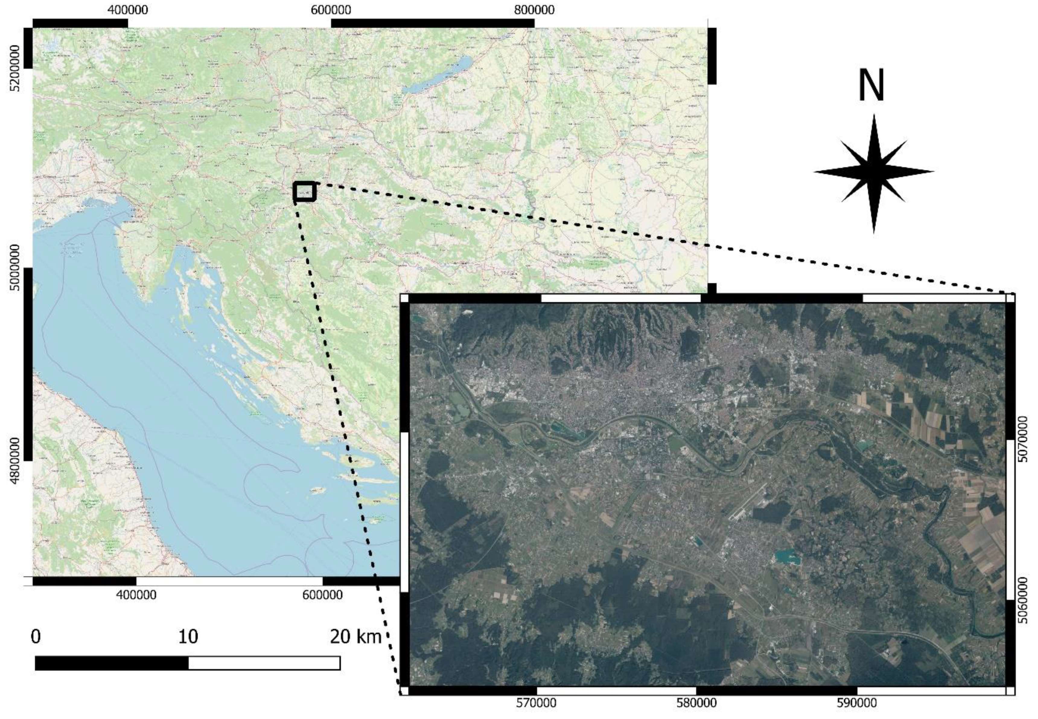
2.1. Study Area and Satellite Data

The study area covers the wider urban area of Zagreb, the largest town in Croatia, including part of Medvednica mountain on the north (Figure 1). The study area is approximately 35 × 21 km with various land cover and land use areas from artificial objects, bare ground, water to low and high vegetation.
The research was conducted on freely available satellite imagery obtained using ESA Sentinel-2 satellite mission. Sentinel-2 satellite mission currently comprises two satellites: Sentinel-2A (S2A), launched on 23 June 2015 and Sentinel-2B (S2B) launched on 7 March 2017. Their constellation provides 5 days’ revisit time. Both satellites have multispectral instrument (MSI) which collects 13 spectral bands: coastal blue, blue, green, red, three vegetation red-edge (RE) bands, near-infrared (NIR), narrow near-infrared, water vapor, shortwave infrared – cirrus and two shortwave infrared (SWIR) bands. Sentinel mission provides two types of products: Level-1C which represents TOA reflectance; and Level-2A which represents Bottom of the atmosphere (BOA) reflectance [3].
For this research, twelve Level-1C images are acquired, six in 2017 and six in 2018 (Table 1). Those images were chosen to obtain unbiased information for classification for two years at similar day of the year. Products and generated maps are projected in WGS84 UTM33 projection, while spatial resolution of used bands was 10 and 20 m.
After the acquisition of 12 Sentinel-2 images, 10 bands frequently used in the land application: blue, green, red, two NIR, three vegetation RE and two SWIR, were chosen for further investigation. Additionally, those bands were chosen because of the spatial resolution of 10 meters (blue, green, red, one NIR) and 20 meters (one NIR, two SWIR and three RE). They were further used in preprocessing and classification. Preprocessing steps include TOA reflectance calculation, five atmospheric corrections, resampling 20 m bands to 10 m resolution and calculation of radiometric indices (Figure 2).

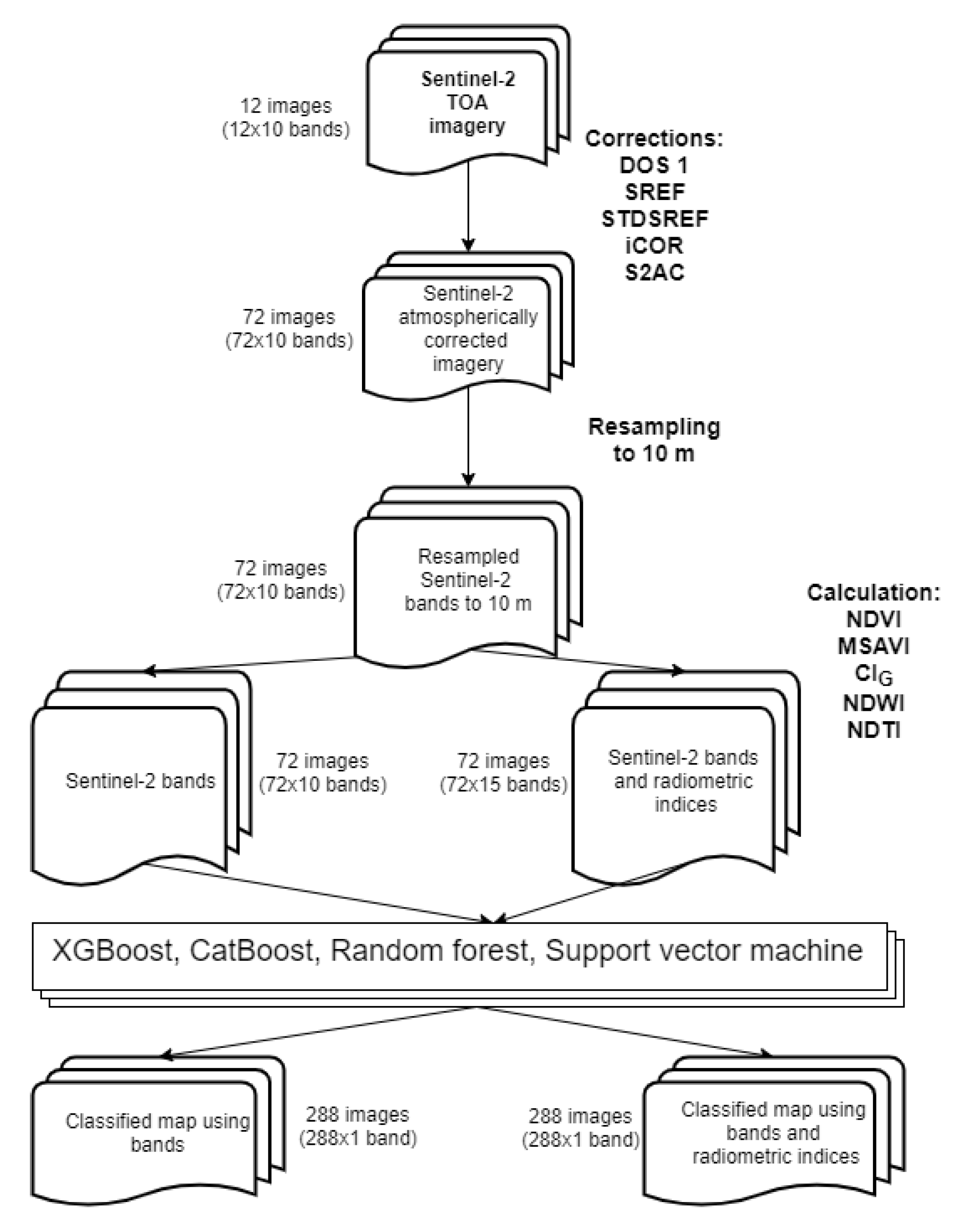
2.2. Processing Workflow

Sentinel-2 imagery processing workflow used in this research is displayed in Figure 2. The first step is the division of twelve Sentinel-2 images with quantification value to obtain TOA reflectance values. The second step is the atmospheric correction of TOA reflectance images using five different atmospheric corrections, which results in 72 images. After atmospheric correction, spectral bands with 20 m resolution was resampled to 10 m. A further step was the calculation of five radiometric indices and the preparation of two datasets for classification. Two datasets, one with Sentinel-2 bands and radiometric indices and one with Sentinel-2 bands, were classified using four classification methods. Finally, classified maps were evaluated using overall and balanced accuracy.

2.3. Atmospheric Corrections

The first step in atmospheric correction procedure is the division of satellite image values with quantification value of 1000 to obtain TOA reflectance [16]. TOA reflectance is the amount of reflectance reflected off the surface which can be collected using a satellite sensor. It has an atmospheric effect included in the measurement, so it is necessary to atmospherically correct this measurement [9].
Atmospheric correction is procedure for correcting satellite imagery from raw data to the bottom of the atmosphere reflectance. This reflectance should be the same as reflectance measured at ground level. There are numerous atmospheric corrections, and for this research, five different atmospheric corrections were used: S2AC, iCOR, DOS, SREF and STDSREF. Atmospheric corrections were conducted using Sen2Cor (v2.5.5) [17] and Atmospheric and Radiometric Correction of Satellite Imagery (ARCSI) software (v3.2.2) [18]. Resampling was conducted using ESA SNAP software (v7.0.1) [19] using the S2 Resampling Processor.

2.3.1. S2AC

S2AC is an atmospheric correction algorithm for calculating the BOA using Sentinel-2 TOA reflectance. S2AC is based on Atmospheric/Topographic Correction for Satellite Imagery (ATCOR) algorithm which was developed in 2011 by Richter [20]. For the computation of atmospheric effects such as solar and thermal radiation S2AC uses Libradtran radiative transfer model [21]. Radiative transfer in Earth’s atmosphere is used for modeling S2AC using simple Lambert (isotropic) law [22]. In this research we did not use Sentinel-2 L2A BOA products because when we processed images, BOA products were not available for all dates. We wanted to have an identically processed dataset, so we calculated the L2A product using the Sen2cor algorithm.

2.3.2. iCOR

iCOR atmospheric correction is a generic scene and sensor correction method for water and land pixel correction. It uses image data and precalculated Look-up-tables (LUT) for deriving required parameters for the method. It calculates correction in four steps: (1) identification and distinction of land and water pixels; (2) calculation of Aerosol optical thickness (AOT) which is derived from land pixels using an adapted version of method developed by Guanter [23], and extending to water pixel assuming spatially homogenous atmosphere; (3) adjacency correction which is calculated using similarity environment correction (SIMEC) [24] over water and over land targets user defines fixed range [25]; (4) the radiative transfer equation calculation [26]. For computation time minimalization MODTRAN LUT is used, while additional information for atmospheric correction is solar and viewing zenith and azimuth angle and digital elevation model (DEM) [27].

2.3.3. DOS

DOS method is image-based atmospheric correction. DOS is a simple method that requires relatively little inputs. It can be easily applied to all image data but does not produce the most reliable and consistent results. It is, therefore, the method used when the other methods are not available. The presumption of DOS correction is that there is an object in complete shadow and at the satellite, sensor received radiance is due to atmospheric scattering [28].

2.3.4. SREF

SREF is calculated using 6S, which is a computer code for accurately simulating atmosphere effects [29]. It accounts for target elevation and non-Lambertian surface conditions. For calculation, it needs six different inputs: the atmospheric profile, aerosol profile, ground reflectance, geometry, altitude and sensor wavelength [30]. The atmospheric profile can be chosen from multiple predefined profiles, or by using measured radiosonde measurement. Aerosol profile depends on the aerosol optical depth and makes a significant difference to measured reflectance values. There are two different ground surfaces that can be chosen to model the ground target: Lambertian and bidirectional reflectance distribution function (BRDF). The next parameter is the geometry of selected sensor ie. date, month, year and time of image acquisition and longitude and latitude of image center or solar and view azimuth and zenith angles. The next parameter is the altitude of the sensor during image acquisition and digital elevation model (DEM) for ground surface. The last parameter is the wavelength of the used sensor [29,30]. Using those parameters, it is possible to correct images to the bottom of the atmosphere reflectance.

2.3.5. STDSREF

STDSREF is surface reflectance product normalized for solar and sensor view angles and topography. The atmospheric model along with DEM is used for diffuse illumination calculation and incidence and exitance angles function for vegetation canopy reflectance calculation on terrain slope. This algorithm works for images with a solar elevation between 50 and 70 degrees and spectral range from 0.25 to 4.0 µm. The main advantage of this atmospheric correction is a correction for the dependence of the vegetation reflectance on the slope along with illumination correction [30,31].

2.4. Radiometric Indices

After atmospheric corrections, spectral characteristics of atmospherically corrected images were analyzed based on five land cover classes: bare land, water, low vegetation, built-up land and high vegetation. After analysis radiometric indices were calculated.
Radiometric index is a joint name for vegetation, soil, water and built-up indices. Radiometric indices are a quantitative measure used to measure different properties, such as biomass or vegetation vigor for vegetation indices or built-up land with built-up indices. For this research we used five different radiometric indices: Normalized difference vegetation index (NDVI) [32], Normalized difference water index (NDWI) [33], Modified soil adjusted vegetation index (MSAVI) [34], Chlorophyll index green (CIG) [35] and Normalized difference turbidity Index (NDTI) [36]. Those indices were chosen due to their often used in research [37,38,39] and their applicability for water and land features.

2.5. Land Cover Classification Methods

After atmospheric correction, resampling and radiometric indices calculation, all satellite images were standardized to range between zero and one. After standardization, images were classified using four chosen machine learning methods: RF; XGB, CB, SVM. All aforementioned methods are machine learning methods. Machine learning land cover classification methods are supervised learning classification where the algorithm learns from the input dataset and uses learned data to predict and classify new observation. Five different land cover classes, water, bare land, low vegetation, high vegetation and built-up land, were chosen for image classification. Training and validation polygons were chosen using orthophoto of Croatia [40] and Sentinel-2 satellite imagery for each date to correctly identify changed land. Training and validation polygons for classification and accuracy assessment were the same for all classification methods for the same date. The number of pixels used for training and validation per layer is provided in Table 2. The number of pixels in Table 2 should be multiplied by 10 or 15, which is the number of layers included in classification. For every classification algorithm, 70% of labeled data was used for training and 30% was used for accuracy assessment [41]. The land cover classification was conducted using the R programming language (version 3.6.1).

2.5.1. RF

RF algorithm is a general term for ensemble learning method which operates using a combination of tree-type classifier in such way that each classifier is generated using random vector which has same distribution for all past random vectors, and it is sampled independently from the values of the input vector. After the creation of the determined number of trees, they vote for the most popular class, so the final output is determined by a majority of the vote [42]. For RF two parameters should be given: the number of trees and the number of features in each split [13]. According to Liaw and Wiener [43], a large number of trees provide a stable result. For selection measure for attribute impurity measure with respect to classes, RF uses the Gini index [44]. RF is not sensitive to overfitting or overtraining due to information that resampling is not based on weighting [45]. The package randomForest was used for RF classification. After hyperparameters tuning, it was decided that default parameters for RF classification give the best result.

2.5.2. XGB

XGB is a machine learning method based on gradient boosting. To generate an optimal model, it uses gradient descent on the decision tree. It generates multiple models that are corrected using the previously generated model and generates the final model [46]. It was developed to overcome the limitation of previously developed gradient boosting algorithms, using a new regularization technique for overfitting control. It is computationally very efficient and more robust during model tuning [47]. In this research, package xgboost was used for XGB classification. Several hyperparameters were tuned to obtain the highest accuracy. For objective function, we used “multi:softmax” function, for a step size of boosting step we used value 0.01, for maximum depth of tree we used value 10 and for the number of rounds we used value 200.

2.5.3. CB

CB is a gradient boosting algorithm for handling categorical data using permutation techniques. Random permutation and averaging label value for the example with the same category value are performed on the dataset. This procedure reduces overfitting [48]. The first step of CB is randomly divided dataset to subset, afterward labels are converted to integer numbers. The last step is the transformation of categorical features to numerical [47]. The package catboost was used to classify Sentinel-2 imagery using CB classification. Lost function, depth and number of iterations were change to obtain the highest accuracy. Lost function was set to “MultiClass”, depth to value 5 and number of iterations to number 200.

2.5.4. SVM

SVM is a supervised machine learning method for classification using statistical learning theory It is designed for finding optimal solutions for classification problems using hyperplane fitting which provides the best separation between two classes in multidimensional feature space [49]. This is one of the main advantages of SVM comparing to other machine learning classification algorithms [50]. Kernel is one of the SVM parameters that needs to be chosen. Users can choose between polynomial, the radial basis function and the sigmoid [49]. Training SVM requires two parameters: C, which represents regularization parameter which controls the trade-off between maximizing the margin and minimizing the training error, and γ which represents kernel width which affects class-dividing hyperplane shape smoothing. A large C value could lead to model overfitting, while a low C value could ignore outliers in training data. On the other hand, increasing γ could affect classification accuracy with changing class-dividing hyperplane shape [13,51]. To classify Sentinel-2 images using SVM classification, e1071 package was used. Several classifications with different C and gamma parameters were tested and the parameters which provided the highest accuracy were chosen.C-classification was used as a type of classification with radial kernel. Additionally, gamma and cost parameters were set to 1.

2.6. Accuracy Assessment
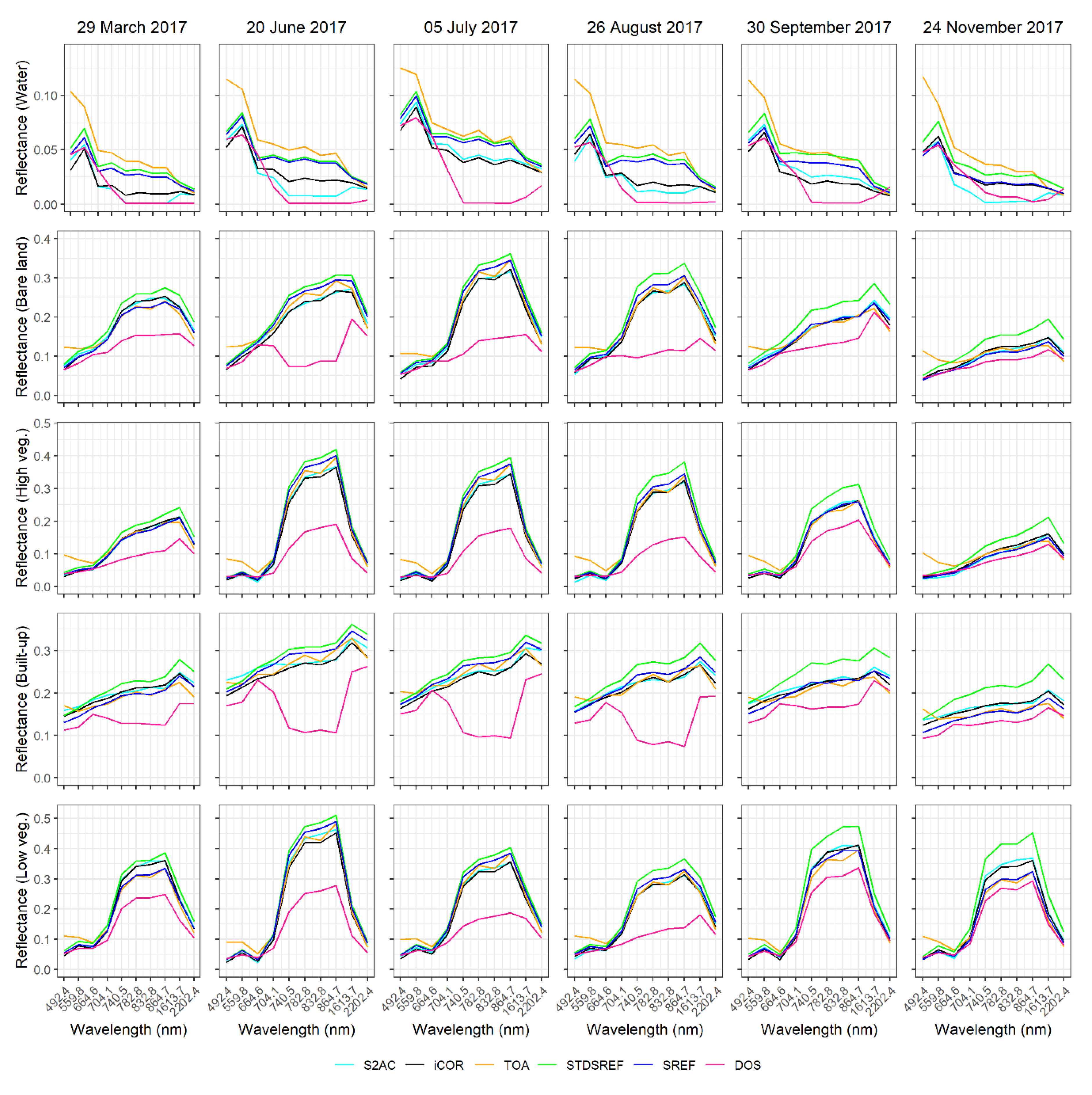
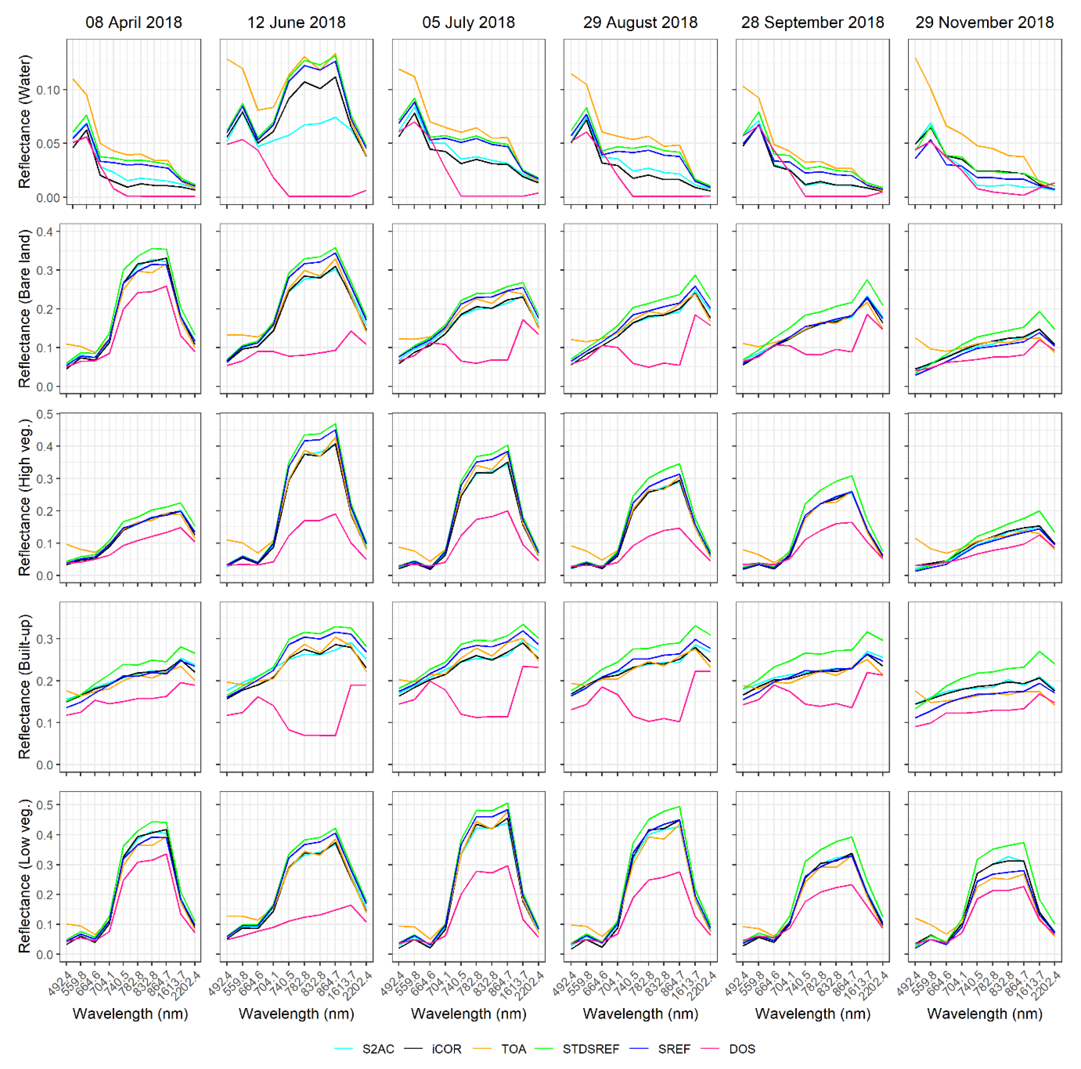
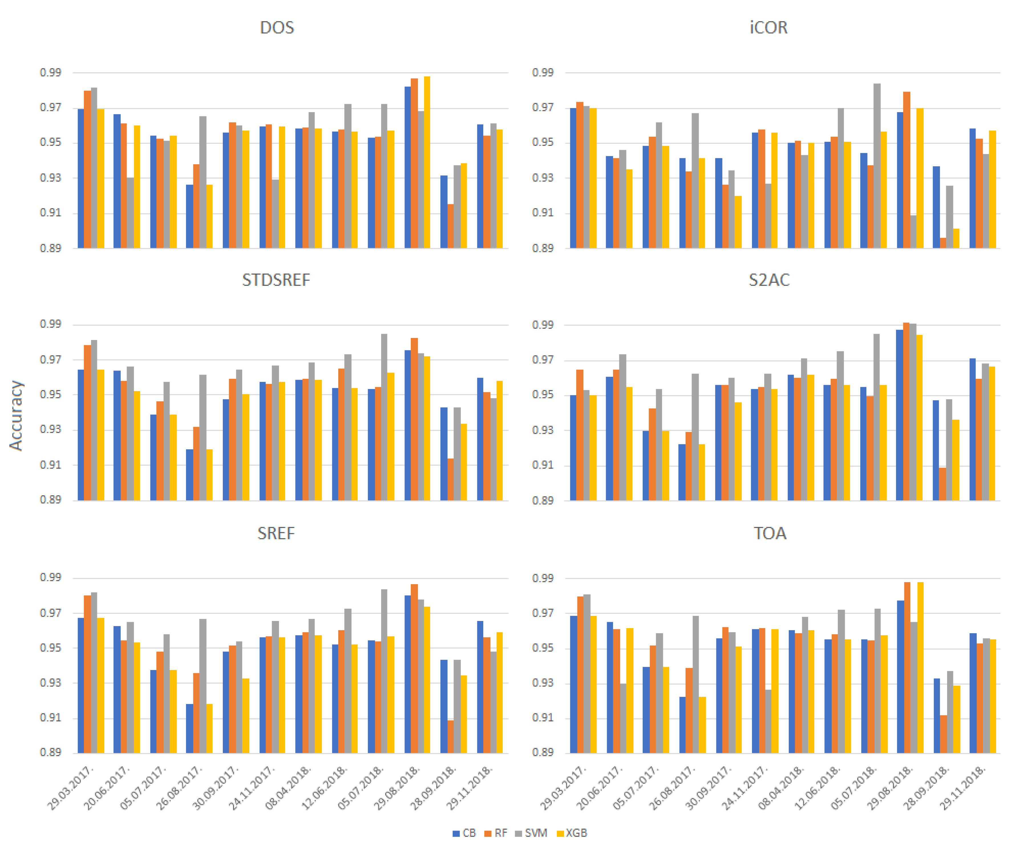
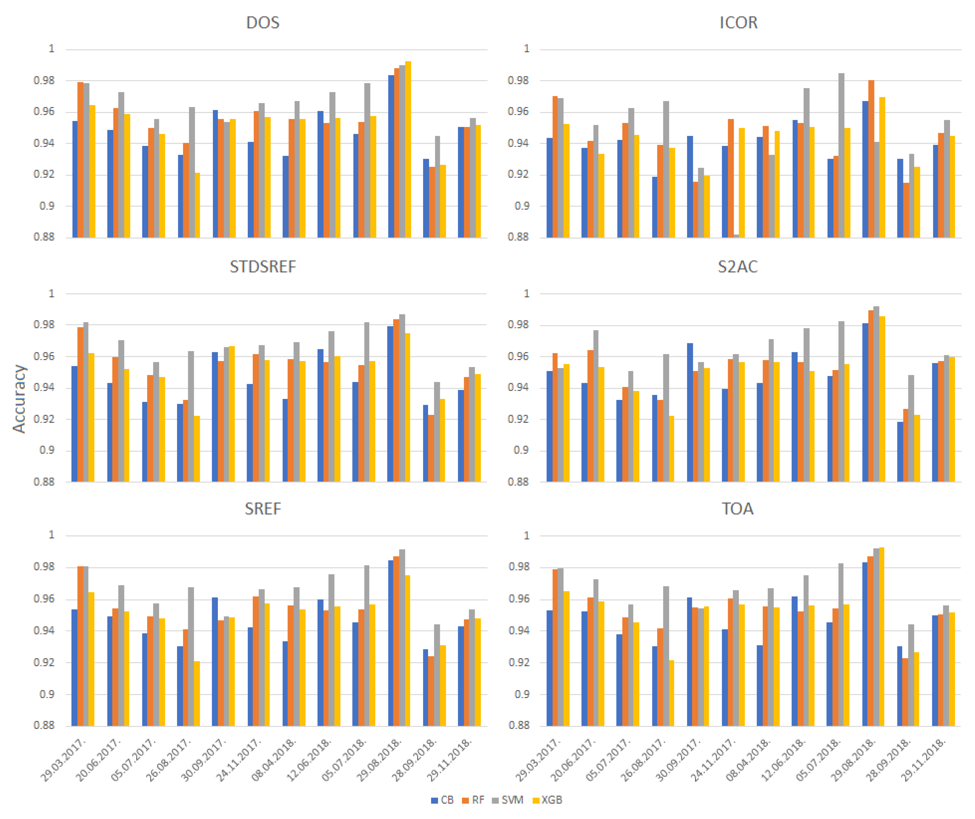
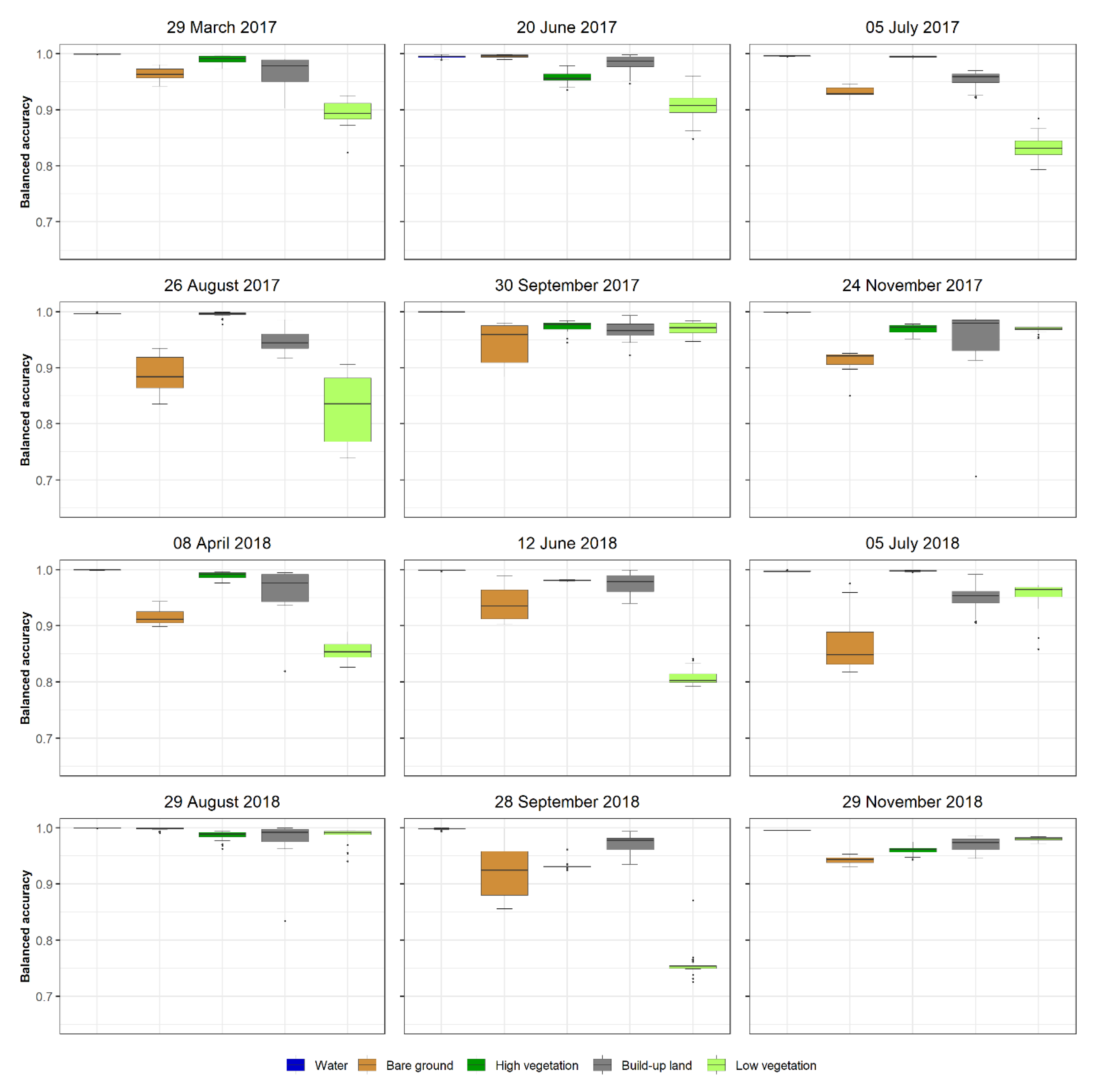
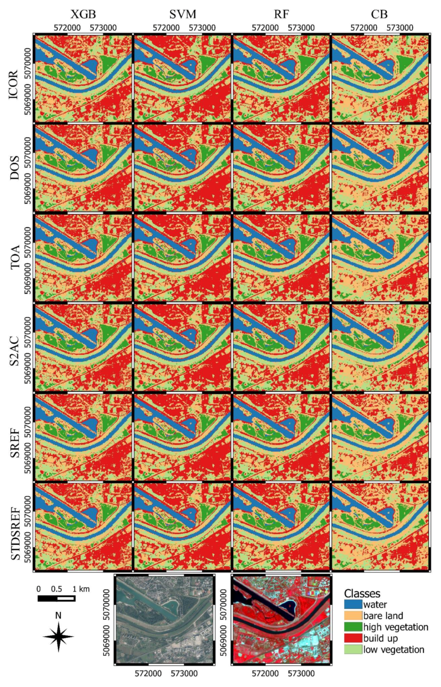
Accuracy assessment was based on the validation dataset, which was not included in the training. Each calculated image was analyzed based on the validation dataset to gain overall accuracy for each image and balanced accuracy for every land cover class. Overall accuracy is the number of correctly classified pixels divided with the total number of items [52]. On the other hand, balanced accuracy can be defined as average accuracy obtained in either class. If the balanced accuracy performs the same in every class, then it represents conventional overall accuracy [53]. For validation, the same samples per date were used for all four classification methods. Furthermore, accuracy for every class for all dates and corrections was also calculated to determine the influence of calculated correction on specific land cover classification class. Classification accuracy was conducted on data with radiometric indices included and without radiometric indices included. Accuracy assessment was conducted using the R programming language (version 3.6.1).
Afterward, all classification accuracies for the same date (24 accuracies per date) were ranked from the highest accuracy, which was ranked as number one, to lowest accuracy, which was ranked as number 24, accordingly. This procedure was repeated for twelve dates and finally summed for all classification methods and atmospheric correction to obtain the best method with the highest accuracy per atmospheric correction and classification method. The best summed result has the lowest number, while the worst result has the highest number.
The last analysis was computational time analysis. The computational time was determined and observed from the training classification algorithm to the end of prediction with obtained prediction results. The computational time depends on the number of stacked layers, where classification time without radiometric indices (10 layers/bands) included is lower than classification time with radiometric indices included (15 layers/bands).

3. Results

A total of 12 Sentinel-2 images was analyzed. After atmospheric correction 72 images were spectrally analyzed. Figure 3 represents spectral signatures of 6 atmospheric corrections for 6 Sentinel-2 images in 2017. The analysis was conducted on 5 different land cover classes: water, bare ground, high vegetation, built-up land and low vegetation using mean value of all training and validation pixels for each class. This resulted in a mean reflectance value for all classes at a specific wavelength. DOS correction has the lowest values for almost all wavelengths and all dates. On the other hand, TOA has the highest values for water class, while STDSREF has the highest value for the other four classes for all dates in 2017.
Figure 4 represents spectral signatures of 6 atmospheric corrections for 6 Sentinel-2 images in 2018. The analysis was conducted the same as for 2017. DOS correction has the lowest values for almost all wavelengths and all dates. On the other hand, TOA has the highest values for water class for visible (red, green blue) and NIR spectrum, while for other bands STDSREF has the highest values. STDSREF has the highest value for bare land, built-up land, high and low vegetation, for all dates in 2018.
After processing steps shown in Figure 2, a total of 576 classified images was calculated and analyzed. Figure 5 shows overall classification accuracy per atmospheric correction method for all twelve dates and four classification methods when using radiometric indices. Overall accuracy for all dates and the atmospheric correction was higher than 89% for all classification methods. SVM has the highest accuracies for all dates except for August 2018 where it is lower than RF classification by 0.04% and for November 2018 where it is 0.28% lower than CB classification. Smallest difference between classification methods is in June 2018 with 2.44% between the lowest and highest overall accuracy, while the biggest margin is in August 2018 with an 8.24% difference. Regarding atmospheric correction, DOS and TOA have similar values with an average difference of 0.40% for all dates. Surface reflectance and Standardized reflectance also have similar values and distribution of values with differences ranging from 0.05% to 1.06% depending on the observed date. S2AC having a similar distribution of values as Surface reflectance and Standardized surface reflectance for almost all dates with differences from 0.02% to 1.74% and 0.05% to 1.63% respectively. Median value for classification methods for all twelve dates are 95.59% for CB, 95.60% for RF, 95.61% for XGB and 96.51% for SVM.
Figure 6 displays classification accuracy of four different methods for images with only ten bands without radiometric indices for twelve dates corrected with six different atmospheric corrections. All classification accuracies for all methods and atmospheric correction are higher than 91%, except for SVM classification of iCOR atmospheric correction for November 2017. The highest overall accuracy is 99.27% in August 2018 for XGB classification of the image with TOA reflectance and image corrected with DOS correction. The lowest classification accuracy is 88.25% for SVM classification of iCOR atmospheric correction in November 2017. Observing other months, SVM has the highest accuracy for all dates except September 2017 and August 2018, where it has lower accuracy by 0.23% from CB and 0.05% from XGB respectively. Median value for classification methods for all twelve dates are 94.35% for CB, 95.39% for XGB, 95.41% for RF and 96.61% for SVM.
Table 3 presents the ranking of each method with included vegetation indices per date (column) from first place (highest accuracy) to twenty-fourth place (lowest accuracy). The last column of Table 3 represents the sum of all rankings for all twelve dates. Better results have lower values and are shown in a darker green color. From Table 3, the SVM method has the lowest summed value for all atmospheric corrections, which means that it is the most accurate classification method for this period.
Table 4 presents the ranking of each method without radiometric indices, per date (column) from first place (highest accuracy) to twenty-fourth place (lowest accuracy). The last column of Table 4 represents the sum of all rankings for all twelve dates. Better results have lower values and are shown in a darker green color. SVM method has the lowest summed value for all atmospheric corrections. All classification for different atmospheric corrections has similar summed values between 52 and 66 for SVM, 133 and 150 for RF, 185 and 208 for CB and 142 and 180 for XGB, while iCOR correction rank stands out.
Figure 7 presents box plots of classification accuracies for five different land cover classes without using radiometric indices. Results are presented as combined values for all atmospheric corrections for twelve dates. Water class does not have a dispersion of classification accuracy for all dates, as well as high vegetation. More dispersed data shows the difference between the classification accuracy of different atmospheric correction. Most differences are between built-up land, bare ground and low vegetation (the points in Figure 7 represent outliers). For March 2017 and April 2018 low vegetation has lower accuracy and built-up land accuracy is dispersed between atmospheric corrections.
Figure 8 presents box plots of classification accuracies for five different land cover classesusing five radiometric indices. Results show similar trends as without radiometric indices that water and high vegetation have low dispersion for all dates and all atmospheric correction. Additionally, low vegetation and bare ground have low dispersion in July 2017, November 2017 and 2018, August 2017 and 2018, but high dispersion in classification accuracy between atmospheric correction in June 2017 and 2018, July 2018 and September 2017 and 2018.
Visual assessments of land cover classification maps on TOA, five different atmospheric corrections: DOS, STDSREF, SREF, iCOR, S2AC and four classification methods: XGB, RF, CB, SVM was conducted on all 576 classified maps for all dates. Figure 9 represents classification maps for 12 June 2018. Figure 9 presents five different classification classes for four different classification methods and six different atmospheric corrections without radiometric indices. Blue color represents water, red urban area, dark green high vegetation, light green low vegetation and orange bare ground. The reference image for visual assessment is orthophoto of Croatia for the year 2017 and Sentinel-2 false-color composite for June 2018.
There are slight differences between classified images. The biggest difference is for images classified with CB algorithm where the algorithm has problems with built-up land and artificial land. XGB also has slight problems with the same two classification classes but on a much smaller scale. Visually SVM provides the best image with a smoother transition between classes and the best representation of the real world.
The computational time depends on the number of stacked layers, where classification time without radiometric indices included (10 layers) is lower than classification time with radiometric indices included (15 layers). Difference without and with radiometric indices is ranging from 0.53 min for CB classification to 4.71 minutes for SVM classification method. Comparing classification method, CB is the fastest method with 1.69 min for classification with radiometric indices and 1.16 minutes without, followed by XGB with 3.63 and 1.90 minutes respectively, the third method is RF with 8.26 and 7.23 minutes and the slowest method is SVM with 39.34 minutes for classification with radiometric indices and 34.63 minutes without. All computational time includes training and prediction for all classification methods (Figure 10).

4. Discussion

The first step in this research was atmospheric correction using five different algorithms: S2AC, iCOR, DOS, SREF and STDSREF. After atmospheric correction images were resampled to 10 meters resolution. This research did not examined the influence of resampling on classification accuracy, because Hunt et al. [54] concluded that 10 m model has higher accuracy than 20 m model when using Sentinel-2 data and RF regression for yield estimation. Furthermore, we used data standardization because Shanker et al. [55] analyzed three data standardization techniques and their results suggest that standardized data yields better general results but slows down computation in terms of computation time.
The first analysis was the spectral analysis of reflectance values for ten Sentinel-2 bands used in this research. The analysis was conducted on all twelve dates for five land cover classes used for classification. From this analysis, it is clear that DOS correction has the lowest value for almost all the wavelengths and all land cover classes. This is expected because DOS is the image-based method. On the other hand, SREF, STDSREF; TOA, iCOR and S2AC have similar values. In 2017, TOA has the highest value for all dates for all of the wavelengths except for SWIR bands. This is expected because water almost has no reflectance in the SWIR band [56]. STDSREF has the highest reflectance value of bare soil, high vegetation, low vegetation and built-up land for all dates in two NIR, three RE and two SWIR bands, while TOA has highest values for blue, green and at certain dates for red. Spectral plot shows that on March 2017 bare land and low vegetation have similar values, so that is one of the reason for lower balanced accuracy. A similar thing happened in June 2017, where the high and low vegetation have very similar spectral values and classifiers have slightly lower accuracy for those classes. In June 2018 the bare land had similar spectral values as the built-up land, as well as low and high vegetation respectively. This resulted in lower classification accuracy for all classes except water. The spectral signature has high influence on classification accuracy and atmospheric correction have impact on band spectral values
Machine learning classification algorithms are influenced by atmospheric correction because it changes surface reflectance values. The main difference in classification results using a machine learning method is a different algorithm definition. Noi and Kappas [13] researched the influence of imbalanced and balanced training dataset for land cover classification and concluded that SVM has the highest accuracy, while RF often has lower accuracy for imbalanced dataset. They also determined that RF performs differently for different satellite datasets. In this research, we concluded the same as Noi and Kappas [13], that SVM has the highest accuracy and in our case, RF has a slightly lower accuracy than SVM. Bhagwat and Shankar [57] analyzed the XGB performance of multilabel remote sensing data and concluded that XGB performed better than RF on the imbalanced dataset. In our research, RF performed better than XGB. A possible reason for the difference in machine learning algorithms could be the choice of user-defined hyperparameters selection. Hyperparameter optimization for all machine learning methods was based on iterative tuning without empirical examination of optimal values.
This research analyzed the influence of radiometric indices on classification accuracy. Castro Gomez [14] analyzed the influence of NDVI, CIG, NDWI and Enhanced vegetation index 2 on classification accuracy using RF classification and Sentinel-2 image. His result shows that Sentinel-2 results have higher accuracy using vegetation indices than results without them. Our results show that on a single date, RF can have higher accuracy with radiometric indices than without them. But when observing twelve dates, classification accuracy is higher without radiometric indices included. The accuracy obtained in this research has higher accuracy ranging from 88.25% to 99.27% without radiometric indices included and between 89.62% to 99.13% with radiometric indices. Close et al. [15] researched the use of Sentinel-2 and LUCAS dataset for classification accuracy using maximum likelihood, RF, k-nearest neighbor, and minimum distance classifier. They classified five different classes: forest land, cropland, grassland, wetlands and settlements and achieved an overall accuracy of 91.1% using maximum likelihood classifier. Our research achieved an accuracy of 99.27% on water, high and low vegetation, bare land and built-up land classes. This research has a similar conclusion Abdi [12] who performed analysis and performance of three machine learning algorithms: SVM, RF, XGB and deep learning algorithm in complex boreal landscapes. Abdi [12] achieved classification accuracy ranging from 73.3% for deep learning to 75.8% for SVM. Our research also achieved the highest accuracy with the SVM classification algorithm.
Vanonckelen et al. [10] evaluated the effect of coupled correction methods on land use/land cover classification accuracy. They used three atmospheric and five topographic corrections for two Landsat images. They used data without atmospheric correction, DOS object subtraction correction and correction based on transmittance for atmospheric correction and data without topographic correction, band rationing, cosine correction, pixel-based Minnaert and pixel-based C-correction topographic corrections. This resulted in fifteen land cover maps which were statistically evaluated based on two validation sets. They used the maximum likelihood classifier based on Gaussian distribution. Their results indicate that atmospheric correction has a low influence on classification results between two dates, which is expected due to small variation in atmospheric parameters. This conclusion is similar to conclusion obtained in our research that some atmospheric correction has a low influence on classification accuracy, but others, such has iCOR, can provide very different and lower classification accuracy than other methods.
The result for classification with and without radiometric indices indicates that the SVM classification method gives the best overall accuracy for all twelve dates in two years. SVM classification has the best results for all atmospheric corrections for both cases (with and without radiometric indices). Depending on the inclusion or exclusion of radiometric indices, the best result is obtained with STDSREF and S2AC accordingly. This result was expected due to the fact that SVM provided the best result in the research of Noi and Kappas [10]. SVM is designed for finding optimal solutions for classification problems using hyperplane fitting which provides the best separation between two classes in multidimensional feature space, which is one of the main advantages of SVM comparing to other machine learning classification algorithms [49,50]. This advantage was confirmed in our research, with SVM having the highest accuracy and best distinction between land cover/use classes. Analyzing CB, RF and XGB classification with radiometric indices included, it can be seen that CB has the best overall accuracy for iCOR and S2AC atmospheric correction, RF has the best overall accuracy for SREF, STDSREF and TOA corrections, while XGB has the best overall accuracy for DOS atmospheric correction. Classification results without radiometric indices are quite different. RF classification method has the best overall accuracy for all atmospheric corrections when compared to CB and XGB. Furthermore, XGB is second best and CB is the worst for all atmospheric correction on twelve dates. One of the reasons for CB performance is sensitivity to hyperparameters selection, which was not fully analyzed in this research. Further, XGB performs better on a larger dataset, while RF performs better for smaller datasets. This can lead to the conclusion that our dataset was too small for XGB and it needs more data to perform better and achieve better overall accuracy. Another reason can be mathematical structure of the algorithm which leads to RF being more regularized than XGB.
The ranking sum for SVM classification indicates that all values except S2AC are much lower (better) for classification without radiometric indices than those with radiometric indices included. This result is the same as Hunt et al. [54] who analyzed if calculation of separate vegetation indices adds extra value for estimation model and concluded that radiometric indices do not add any extra value to model, but can even lower the accuracy of certain classification techniques. The ranking sum for RF, DOS correction has the same ranking with and without radiometric indices, while iCOR and TOA have a slightly better rank for classification without radiometric indices. The ranking of XGB classifier is better with radiometric indices for TOA, DOS, iCOR and S2AC atmospheric correction and better without radiometric indices for SREF and STDSREF. The ranking of CB classifier on the other hand, has a much better result when using radiometric indices, then without using radiometric indices.
All classification methods have the lowest ranking for iCOR atmospheric correction. One of the reasons is that iCOR has been developed for land and water features correction. One of the algorithm limitations is difficulty in the derivation of reliable aerosol model estimation and the assumption that surface reflectance should be displayed as a linear combination of two pure green vegetation and a bare soil endmember. Another limitation of iCOR is that it does not correct the image for sun glint effects [26]. SREF and STDSREF perform well only with SVM classification with and without radiometric indices and partially for XGB classification with STDSREF atmospheric correction. One of the reasons is that SVM is using hyperplane fitting with the best distinction between classes. CB, RF and XGB achieved best results for images with TOA reflectance and corrected using DOS correction with and without radiometric indices included.
Low vegetation and bare ground are two land cover classes that influence the classification accuracy the most. In spring months March 2017 and April 2018 low vegetation has the lowest balanced accuracy and affects the overall classification accuracy the most. This is expected because high vegetation is still not growing, while water and the built-up area do not change. Low vegetation reflectance is higher because the phenology cycle starts earlier than the high vegetation cycle so the classifiers can mix high and low vegetation. This can lead to the false classification which can lower accuracy. This is the case for classification with radiometric indices and without it. Water, high vegetation and built-up land have similar classification accuracy in July 2017 and 2018. In July 2018 bare ground has lower and more dispersed accuracy and low vegetation has higher accuracy than in July 2017. Those differences are mainly due to different reflectance values because of different weather conditions in 2017 and 2018. In July 2017 it was extremely hot and dry, while in 2018 it was a normal condition for the Zagreb area. Another reason can be a lower number of samples for bare ground in July 2018 which influence classification algorithms which can be seen on the dispersion of results in July 2018. November 2017 and 2018 have very similar balanced accuracy for all classes with a slight difference in low vegetation. In August 2018 differences are in bare land, low vegetation and built-up land classes. All classes had very high accuracy in August 2018. In August 2017 it was extremely hot and dry, while in 2018 it was extremely hot, but with normal rain conditions. In September 2017 and 2018 the difference is in classes bare soil, high and low vegetation. One of the reasons could be different weather which was cold and very rainy in September 2017 and very warm and dry in 2018.
The difference in the accuracy of classes without radiometric indices is in the same months as with radiometric indices included, with one difference in June 2017 and 2018, where there is slightly lower accuracy for built-up land in 2017 and for bare ground in 2018. One of the reasons is similar spectral reflectance values that can occur and confuse the classification algorithm. Radiometric indices have an impact on ranking, and respectively overall accuracy, of classification methods. By observing classification for every date, the biggest difference in ranking between classification, which included radiometric indices and without it, is in November 2017 and 2018.
Ranking by single date shows that radiometric indices or lack of those, influence different dates. For SVM classification of DOS atmospheric correction with radiometric indices there are four dates with ranking lower than 10. Those are 20. June 2017, 24 November 2017 and 29 August 2018. On the other hand, classification without radiometric indices provides only one ranking lower than 10 on 30. September 2017. This shows that algorithm performs differently with or without radiometric indices which confirms previous researches that feature selection is very important [58,59,60] and there should not be redundancy (feature correlation) in different layers [61].
Balanced classification accuracies of land cover classes are similar when classified with radiometric indices and without them. The biggest difference is in April and September 2018. In April built-up land has similar accuracy for all atmospheric correction with radiometric indices, while without radiometric indices results are more dispersed. In September 2018, the difference is in bare ground class, where balanced accuracies are sparse for classifications with radiometric indices included than without them. Those differences are mostly due to, as previously stated, feature selection and feature correlation, which influence classification results.
The area around Jarun lake in Zagreb was chosen for visual assessment because it has a heterogeneous land cover. Orthophoto of Croatia for the year 2017 was used as the reference image. Visually comparing images by atmospheric correction, it can be seen that CB classification classified built-up land and low vegetation as bare land classes. XGB and RF also classified low vegetation and built-up land as bare land but in a much smaller margin. All classifiers have problems with lower vegetation, as part of low vegetation is classified as high vegetation, due to time of the growing season, and part of the vegetation is classified as bare land.
Classification processing time is very different for all classification methods. SVM is the slowest classification method almost 5 times slower than RF. RF is 4 times slower than XGB when radiometric indices are included and 2 times slower without radiometric indices. CB is the fastest algorithm. It is 1.5× faster than XGB without radiometric indices included and 2× faster with radiometric indices included. If comparing accomplished accuracy and time of classification without radiometric indices included, the fastest method has the lowest accuracy, while the slowest method has the highest accuracy. The slowest classification method with radiometric indices is SVM, but it has the highest overall accuracy. RF, as the second slowest method, has the second highest accuracy for TOA and two atmospheric corrections: SREF and STDSREF. CB as the fastest method has the second-best classification accuracy for two atmospheric corrections (S2AC and iCOR) and XGB has the best accuracy for just one atmospheric correction method (DOS).

5. Conclusions

Influence of five atmospheric corrections, namely S2AC, iCOR, DOS, SREF, STDSREF, on five machine learning classification algorithms, SVM, RF, XGB, CB was examined. SVM classification method outperformed all other methods with radiometric indices included, but also without included radiometric indices for all twelve dates. The overall accuracy of SVM was between 90.89% for iCOR correction and 99.09% for S2AC with the median value of 96.51%, depending on a date with radiometric indices included and between 88.25% for iCOR and 99.22% for TOA without radiometric indices included. SVM classification was the best for all atmospheric correction. For classification with radiometric indices included SVM performed the best for S2AC with the median value of 96.54%, while for classification without radiometric indices SVM performed the best for STDSREF with median value of 96.83%. The ranking is better without radiometric indices for SVM and RF but lower for XGB and CB.
This study showed and verified that SVM is the best machine learning classifier for land cover/use classification and outperformed RF, CB and XGB. On the other hand, SVM was the slowest algorithm in means of computational time needed for classification, while RF and XGB were faster and CB the fastest machine learning method. So, when the time is of the essence, this should be considered. This research concluded that the selection of classifiers is the most important, while the selection of atmospheric correction method is, apart from iCOR correction, is of minor importance although they change spectral values of satellite images.
One of the most important aspects of this research is the fact that all the atmospheric correction and machine learning classification methods are freely available, along with the Sentinel-2 dataset.
Our research was conducted on a specific study site of the City of Zagreb in 2017 and 2018, so further work should consider including more atmospheric corrections, new study sites, different years and multitemporal classification with all dates included.

Author Contributions

Conceptualization, Mario Miler and Luka Rumora; methodology, Luka Rumora; software, Luka Rumora; validation, Mario Miler; writing—original draft, Luka Rumora.; writing—review and editing, Mario Miler; visualization, Luka Rumora and Mario Miler; supervision, Damir Medak; funding acquisition, Damir Medak. All authors have read and agreed to the published version of the manuscript.

Funding

This research was supported by the Croatian Science Foundation under the projects HRZZ-IP-2016-06-5621 “Geospatial Monitoring of Green Infrastructure by Means of Terrestrial, Airborne and Satellite Imagery (GEMINI)”.

Conflicts of Interest

The authors declare no conflict of interest.

References

  1. Chrysoulakis, N.; Abrams, M.; Feidas, H.; Arai, K. Comparison of atmospheric correction methods using ASTER data for the area of Crete, Greece. Int. J. Remote Sens. 2010, 31, 6347–6385. [Google Scholar] [CrossRef]
  2. Claverie, M.; Ju, J.; Masek, J.G.; Dungan, J.L.; Vermote, E.F.; Roger, J.C.; Skakun, S.V.; Justice, C. The Harmonized Landsat and Sentinel-2 surface reflectance data set. Remote Sens. Environ. 2018, 219, 145–161. [Google Scholar] [CrossRef]
  3. Lantzanakis, G.; Mitraka, Z.; Chrysoulakis, N. Comparison of physically and image based atmospheric correction methods for Sentinel-2 satellite imagery. In Proceedings of the Fourth International Conference on Remote Sensing and Geoinformation of the Environment (RSCy2016), Paphos, Cyprus, 4–8 April 2016; Volume 9688, p. 96880A. [Google Scholar]
  4. Adam, E.; Mutanga, O.; Odindi, J.; Abdel-Rahman, E.M. Land-use/cover classification in a heterogeneous coastal landscape using RapidEye imagery: evaluating the performance of random forest and support vector machines classifiers. Int. J. Remote Sens. 2014, 35, 3440–3458. [Google Scholar] [CrossRef]
  5. Koc-San, D. Evaluation of different classification techniques for the detection of glass and plastic greenhouses from WorldView-2 satellite imagery. J. Appl. Remote Sens. 2013, 7, 073553. [Google Scholar] [CrossRef]
  6. Sonobe, R.; Yamaya, Y.; Tani, H.; Wang, X.; Kobayashi, N.; Mochizuki, K. ichiro Assessing the suitability of data from Sentinel-1A and 2A for crop classification. GIScience Remote Sens. 2017, 54, 918–938. [Google Scholar] [CrossRef]
  7. Ballanti, L.; Blesius, L.; Hines, E.; Kruse, B. Tree species classification using hyperspectral imagery: A comparison of two classifiers. Remote Sens. 2016, 8, 445. [Google Scholar] [CrossRef] [Green Version]
  8. Liang, S.; Fang, H.; Chen, M. Atmospheric correction of Landsat ETM+ land surface imagery-Part I: Methods. IEEE Trans. Geosci. Remote Sens. 2001, 39, 2490–2498. [Google Scholar] [CrossRef]
  9. Rumora, L.; Miler, M.; Medak, D. Contemporary comparative assessment of atmospheric correction influence on radiometric indices between Sentinel-2A and Landsat 8 imagery. Geocarto Int. 2019, 1–15. [Google Scholar] [CrossRef]
  10. Vanonckelen, S.; Lhermitte, S.; Van Rompaey, A. The effect of atmospheric and topographic correction methods on land cover classification accuracy. Int. J. Appl. Earth Obs. Geoinf. 2013, 24, 9–21. [Google Scholar] [CrossRef] [Green Version]
  11. Lin, C.; Wu, C.C.; Tsogt, K.; Ouyang, Y.C.; Chang, C.I. Effects of atmospheric correction and pansharpening on LULC classification accuracy using WorldView-2 imagery. Inf. Process. Agric. 2015, 2, 25–36. [Google Scholar] [CrossRef] [Green Version]
  12. Abdi, A.M. Land cover and land use classification performance of machine learning algorithms in a boreal landscape using Sentinel-2 data. GIScience Remote Sens. 2020, 57, 1–20. [Google Scholar] [CrossRef] [Green Version]
  13. Noi, P.T.; Kappas, M. Comparison of random forest, k-nearest neighbor, and support vector machine classifiers for land cover classification using sentinel-2 imagery. Sensors (Switzerland) 2017, 18. [Google Scholar]
  14. Castro Gomez, M.G. Joint use of Sentinel-1 and Sentinel-2 for land cover classification: A machine learning approach. Lund Univ. GEM thesis Ser. 2017, NGEM01, 20162. [Google Scholar]
  15. Close, O.; Benjamin, B.; Petit, S.; Fripiat, X.; Hallot, E. Use of Sentinel-2 and LUCAS database for the inventory of land use, land use change, and forestry in Wallonia, Belgium. Land 2018, 7, 154. [Google Scholar] [CrossRef] [Green Version]
  16. Traganos, D.; Poursanidis, D.; Aggarwal, B.; Chrysoulakis, N.; Reinartz, P. Estimating satellite-derived bathymetry (SDB) with the Google Earth Engine and sentinel-2. Remote Sens. 2018, 10, 859. [Google Scholar] [CrossRef] [Green Version]
  17. Sen2Cor Software Release Note. Available online: http://step.esa.int/thirdparties/sen2cor/2.5.5/docs/S2-PDGS-MPC-L2A-SRN-V2.5.5.pdf. (accessed on 9 April 2020).
  18. Bunting, P.; Clewley, D. Atmospheric and Radiometric Correction of Satellite Imagery (ARCSI). Available online: https://www.arcsi.remotesensing.info/. (accessed on 9 April 2020).
  19. ESA SNAP. Available online: https://step.esa.int/main/toolboxes/snap/ (accessed on 9 April 2020).
  20. Richter, R.; Schlapfer, D.; Muller, A. Operational atmospheric correction for imaging spectrometers accounting for the smile effect. IEEE Trans. Geosci. Remote Sens. 2011, 49, 1772–1780. [Google Scholar] [CrossRef]
  21. Emde, C.; Buras-Schnell, R.; Kylling, A.; Mayer, B.; Gasteiger, J.; Hamann, U.; Kylling, J.; Richter, B.; Pause, C.; Dowling, T.; et al. The libRadtran software package for radiative transfer calculations (version 2.0.1). Geosci. Model Dev. 2016, 9, 1647–1672. [Google Scholar] [CrossRef] [Green Version]
  22. Toming, K.; Kutser, T.; Laas, A.; Sepp, M.; Paavel, B.; Nõges, T. First experiences in mapping lakewater quality parameters with sentinel-2 MSI imagery. Remote Sens. 2016, 8, 640. [Google Scholar] [CrossRef] [Green Version]
  23. Guanter, L. New algorithms for atmospheric correction and retrieval of biophysical parameters in Earth Observation; Application to ENVISAT / MERIS data, University of Valencia: Valencia, Spain, 2006. [Google Scholar]
  24. Sterckx, S.; Knaeps, E.; Adriaensen, S.; Reusen, I.; De Keukelaere, L.; Hunter, P. Opera: An Atmospheric Correction for Land and Water. Proc. Sentin. Sci. Work. 2015, 1, 3–6. [Google Scholar]
  25. König, M.; Hieronymi, M.; Oppelt, N. Application of sentinel-2 msi in arctic research: Evaluating the performance of atmospheric correction approaches over arctic sea ice. Front. Earth Sci. 2019, 7, 22. [Google Scholar] [CrossRef] [Green Version]
  26. De Keukelaere, L.; Sterckx, S.; Adriaensen, S.; Knaeps, E.; Reusen, I.; Giardino, C.; Bresciani, M.; Hunter, P.; Neil, C.; Van der Zande, D.; et al. Atmospheric correction of Landsat-8/OLI and Sentinel-2/MSI data using iCOR algorithm: validation for coastal and inland waters. Eur. J. Remote Sens. 2018, 51, 525–542. [Google Scholar] [CrossRef] [Green Version]
  27. Pereira-Sandoval, M.; Ruescas, A.; Urrego, P.; Ruiz-Verdú, A.; Delegido, J.; Tenjo, C.; Soria-Perpinyà, X.; Vicente, E.; Soria, J.; Moreno, J. Evaluation of atmospheric correction algorithms over spanish inland waters for sentinel-2 multi spectral imagery data. Remote Sens. 2019, 11, 1469. [Google Scholar] [CrossRef] [Green Version]
  28. Chavez, P.S. Image-based atmospheric corrections - Revisited and improved. Photogramm. Eng. Remote Sens. 1996, 62, 1025–1036. [Google Scholar]
  29. Vermote, E.F.; Tanré, D.; Deuzé, J.L.; Herman, M.; Morcrette, J.J. Second simulation of the satellite signal in the solar spectrum, 6s: an overview. IEEE Trans. Geosci. Remote Sens. 1997, 35, 675–686. [Google Scholar] [CrossRef] [Green Version]
  30. Bunting, P. Introduction to ARCSI for generating Analysis Ready Data (ARD). Available online: https://www.arcsi.remotesensing.info/tutorials/ARCSI_Intro_Tutorial_compress.pdf (accessed on 9 April 2020).
  31. Shepherd, J.D.; Dymond, J.R. Correcting satellite imagery for the variance of reflectance and illumination with topography. Int. J. Remote Sens. 2003, 24, 3503–3514. [Google Scholar] [CrossRef]
  32. Baret, F.; Guyot, G.; Major, D.J. Crop biomass evaluation using radiometric measurements. Photogrammetria 1989, 43, 241–256. [Google Scholar] [CrossRef]
  33. McFeeters, S.K. The use of the Normalized Difference Water Index (NDWI) in the delineation of open water features. Int. J. Remote Sens. 1996, 17, 1425–1432. [Google Scholar] [CrossRef]
  34. Qi, J.; Chehbouni, A.; Huete, A.R.; Kerr, Y.H.; Sorooshian, S. A modified soil adjusted vegetation index. Remote Sens. Environ. 1994, 48, 119–126. [Google Scholar] [CrossRef]
  35. Godinho, S.; Guiomar, N.; Gil, A. Using a stochastic gradient boosting algorithm to analyse the effectiveness of Landsat 8 data for montado land cover mapping: Application in southern Portugal. Int. J. Appl. Earth Obs. Geoinf. 2016, 49, 151–162. [Google Scholar] [CrossRef]
  36. Lacaux, J.P.; Tourre, Y.M.; Vignolles, C.; Ndione, J.A.; Lafaye, M. Classification of ponds from high-spatial resolution remote sensing: Application to Rift Valley Fever epidemics in Senegal. Remote Sens. Environ. 2007, 106, 66–74. [Google Scholar] [CrossRef]
  37. Belgiu, M.; Csillik, O. Sentinel-2 cropland mapping using pixel-based and object-based time-weighted dynamic time warping analysis. Remote Sens. Environ. 2018, 204, 509–523. [Google Scholar] [CrossRef]
  38. Yang, X.; Zhao, S.; Qin, X.; Zhao, N.; Liang, L. Mapping of urban surface water bodies from sentinel-2 MSI imagery at 10 m resolution via NDWI-based image sharpening. Remote Sens. 2017, 9, 596. [Google Scholar] [CrossRef] [Green Version]
  39. Elhag, M.; Gitas, I.; Othman, A.; Bahrawi, J.; Gikas, P. Assessment of water quality parameters using temporal remote sensing spectral reflectance in arid environments, Saudi Arabia. Water (Switzerland) 2019, 11, 556. [Google Scholar] [CrossRef] [Green Version]
  40. Republic of Croatia, State Geodetic Administration (DGU) Geoportal DGU. Available online: https://geoportal.dgu.hr/ (accessed on 13 January 2020).
  41. Xu, R.; Lin, H.; Lü, Y.; Luo, Y.; Ren, Y.; Comber, A. A modified change vector approach for quantifying land cover change. Remote Sens. 2018, 10, 1578. [Google Scholar] [CrossRef] [Green Version]
  42. Breiman, L. Random forests. Mach. Learn. 2001, 45, 5–32. [Google Scholar] [CrossRef] [Green Version]
  43. Liaw, A.; Wiener, M. Classification and Regression by randomForest. R News 2002, 2, 18–22. [Google Scholar]
  44. Pal, M. Random forest classifier for remote sensing classification. Int. J. Remote Sens. 2005, 26, 217–222. [Google Scholar] [CrossRef]
  45. Gislason, P.O.; Benediktsson, J.A.; Sveinsson, J.R. Random forests for land cover classification. Pattern Recognition Lett. 2006, 27, 294–300. [Google Scholar] [CrossRef]
  46. Chen, T.; Guestrin, C. XGBoost: A scalable tree boosting system. In Proceedings of the Proceedings of the ACM SIGKDD International Conference on Knowledge Discovery and Data Mining, San Francisco, CA, USA, 13–17 August 2016. [Google Scholar]
  47. Daoud, E. Al Comparison between XGBoost, LightGBM and CatBoost Using a Home Credit Dataset. Int. J. Comput. Inf. Eng. 2019, 13, 6–10. [Google Scholar]
  48. Prokhorenkova, L.; Gusev, G.; Vorobev, A.; Dorogush, A.V.; Gulin, A. Catboost: Unbiased boosting with categorical features. In Proceedings of the Advances in Neural Information Processing Systems, Montreal, QC, Canada, 2–8 December 2018. [Google Scholar]
  49. Petropoulos, G.P.; Kalaitzidis, C.; Prasad Vadrevu, K. Support vector machines and object-based classification for obtaining land-use/cover cartography from Hyperion hyperspectral imagery. Comput. Geosci. 2012, 41, 99–107. [Google Scholar] [CrossRef]
  50. Huang, C.; Song, K.; Kim, S.; Townshend, J.R.G.; Davis, P.; Masek, J.G.; Goward, S.N. Use of a dark object concept and support vector machines to automate forest cover change analysis. Remote Sens. Environ. 2008, 112, 970–985. [Google Scholar] [CrossRef]
  51. Knorn, J.; Rabe, A.; Radeloff, V.C.; Kuemmerle, T.; Kozak, J.; Hostert, P. Land cover mapping of large areas using chain classification of neighboring Landsat satellite images. Remote Sens. Environ. 2009, 113, 957–964. [Google Scholar] [CrossRef]
  52. Yingqiu, L.; Wei, L.; Yunchun, L. Network traffic classification using K-means clustering. In Proceedings of the Proceedings - 2nd International Multi-Symposiums on Computer and Computational Sciences, IMSCCS’07, Iowa City, IA, USA, 13–15 August 2007; pp. 360–365. [Google Scholar]
  53. Brodersen, K.H.; Ong, C.S.; Stephan, K.E.; Buhmann, J.M. The balanced accuracy and its posterior distribution. In Proceedings of the Proceedings - International Conference on Pattern Recognition, Istanbul, Turkey, 23–26 August 2010; pp. 3121–3124. [Google Scholar]
  54. Hunt, M.L.; Blackburn, G.A.; Carrasco, L.; Redhead, J.W.; Rowland, C.S. High resolution wheat yield mapping using Sentinel-2. Remote Sens. Environ. 2019, 233, 111410. [Google Scholar] [CrossRef]
  55. Shanker, M.S.; Hu, M.Y.; Hung, M.S. Effect of data standardization on neural network training. Omega 1996, 24, 385–397. [Google Scholar] [CrossRef]
  56. Vanhellemont, Q.; Ruddick, K. Advantages of high quality SWIR bands for ocean colour processing: Examples from Landsat-8. Remote Sens. Environ. 2015, 161, 89–106. [Google Scholar] [CrossRef] [Green Version]
  57. Bhagwat, R.U.; Uma Shankar, B. A novel multilabel classification of remote sensing images using XGBoost. In Proceedings of the 2019 IEEE 5th International Conference for Convergence in Technology (I2CT), Bombay, India, 29–31 March 2019. [Google Scholar]
  58. Pal, M.; Foody, G.M. Feature selection for classification of hyperspectral data by SVM. IEEE Trans. Geosci. Remote Sens. 2010, 48, 2297–2307. [Google Scholar] [CrossRef] [Green Version]
  59. Li, X.; Chen, W.; Cheng, X.; Liao, Y.; Chen, G. Comparison and integration of feature reduction methods for land cover classification with RapidEye imagery. Multimed. Tools Appl. 2017, 76, 23041–23057. [Google Scholar] [CrossRef]
  60. Löw, F.; Michel, U.; Dech, S.; Conrad, C. Impact of feature selection on the accuracy and spatial uncertainty of per-field crop classification using Support Vector Machines. ISPRS J. Photogramm. Remote Sens. 2013, 85, 102–119. [Google Scholar] [CrossRef]
  61. Makrehchi, M.; Kamel, M.S. Aggressive Feature Selection by Feature Ranking. In Computational Methods of Feature Selection; Liu, H., Motoda, H., Eds.; CRC Press: Boca Raton, FL, USA, 2007; pp. 313–335. [Google Scholar]
Figure 1. Study area location.
Ijgi 09 00277 g001
Figure 2. The workflow of processing Sentinel-2.
Ijgi 09 00277 g002
Figure 3. Sentinel-2 spectral signatures of five atmospheric corrections and top of the atmosphere (TOA) on five land cover classes for the year 2017.
Ijgi 09 00277 g003
Figure 4. Sentinel-2 spectral signatures of five atmospheric corrections and TOA on five land cover classes for the year 2018.
Ijgi 09 00277 g004
Figure 5. Classification accuracy based on atmospheric correction and date with radiometric indices.
Ijgi 09 00277 g005
Figure 6. Classification accuracy based on atmospheric correction and date without vegetation indices.
Ijgi 09 00277 g006
Figure 7. Box-plot of balanced classification accuracies of land cover classes without radiometric indices for combined atmospheric corrections for twelve dates.
Ijgi 09 00277 g007
Figure 8. Box-plot of balanced classification accuracies of land cover classes with radiometric indices for combined atmospheric corrections for twelve dates.
Ijgi 09 00277 g008
Figure 9. Classification maps for 12 June 2018 for four classification techniques and six atmospheric corrections.
Ijgi 09 00277 g009
Figure 10. Average processing time for all twelve dates for SVM, RF, XGB and CB classification method with and without vegetation indices included.
Ijgi 09 00277 g010
Table 1. Satellite images used in this study.
Sensing DateImage IDSatellite
29.03.2017N0204_R079_T33TWLSentinel-2A
20.06.2017N0205_R122_T33TWLSentinel-2A
05.07.2017N0205_R122_T33TWLSentinel-2B
26.08.2017N0205_R079_T33TWLSentinel-2A
30.09.2017N0205_R079_T33TWLSentinel-2B
24.11.2017N0206_R079_T33TWLSentinel-2A
08.04.2018N0206_R079_T33TWLSentinel-2B
12.06.2018N0206_R079_T33TWLSentinel-2A
05.07.2018N0206_R122_T33TWLSentinel-2A
29.08.2018N0206_R122_T33TWLSentinel-2B
28.09.2018N0206_R122_T33TWLSentinel-2B
29.11.2018N0207_R079_T33TWLSentinel-2A
Table 2. Number of pixels per band for training and validation for all five land cover classes per date.
Sensing DateTraining and Validation Pixels Per Layer
WaterBare SoilHigh VegetationBuilt-up LandLow Vegetation
29.03.201713413204874740077788843
20.06.2017134131351447400458811251
05.07.201713413186404740077789218
26.08.201713413186404740077789107
30.09.201713413206674740045887891
24.11.2017134131466347400777813530
08.04.201813413204874740077789043
12.06.201813413204874740077788843
05.07.201813413896147400777810089
29.08.2018134131010647400458813207
28.09.2018134131635547400458811719
29.11.2018134132764647400458814998
Table 3. Ranking of method and correction by date with included radiometric indices. Ranking is provided by place rank.
2017 2018
Method Date29
03
20
06
05
07
26
08
30
09
24
11
08
04
12
06
05
07
29
08
28
09
29
11
SUM
Correction
SVMDOS2231145223562185115
iCOR10191221232463241724174
SREF15331325341442380
STDSREF4346112221852270
S2AC221854311121251
TOA3242162433523916119
RFDOS6109103716111871818133
iCOR9217122310212024132420204
SREF516141114131281982115156
STDSREF814151371411715101921154
S2AC19616141119109221228157
TOA7111092415101632019126
CBDOS1325159817122111156134
iCOR11201272017222323221011198
SREF178212317151921171234177
STDSREF207192118111318201667176
S2AC23122319102061414621150
TOA154171712581613151410146
XGBDOS131351588171295713125
iCOR11221272417222311202314206
SREF17172123221519211017129203
STDSREF20181921161113187191312187
S2AC231523191920614129113174
TOA1591717155816841617147
Table 4. Ranking of method and correction by date without radiometric indices. Ranking is provided by place rank.
2017 2018
Method Date29
03
20
06
05
07
26
08
30
09
24
11
08
04
12
06
05
07
29
08
28
09
29
11
SUM
Correction
SVMDOS725515346662566
iCOR101713222422412467141
SREF352218233554860
STDSREF14343122495947
S2AC211768511341159
TOA434114455233452
RFDOS578912811201481714133
iCOR9226102416161923182419206
SREF2129820692115111918150
STDSREF7911139761512142120144
S2AC14618151710713167153141
TOA68107139122213102212144
CBDOS1719201452123101915913185
iCOR242317242123181824231123249
SREF19181916719201221131322199
STDSREF1821241841821722191224208
S2AC232023121221981817236192
TOA201521166202492016915191
XGBDOS1210142210141314711411142
iCOR222415112317172317221821230
SREF13141223191215171020817180
STDSREF15161320211811821716148
S2AC16132219161310241112202178
TOA1110162111141415911610148

