Affective Communication of Map Symbols: A Semantic Differential Analysis


Department of Geodesy and Geoinformation, Research Division Cartography, TU Wien—Vienna University of Technology, 1040 Vienna, Austria
ISPRS Int. J. Geo-Inf. 2020, 9(5), 289; https://0-doi-org.brum.beds.ac.uk/10.3390/ijgi9050289
Submission received: 20 March 2020
/
Revised: 19 April 2020
/
Accepted: 22 April 2020
/
Published: 1 May 2020
(This article belongs to the Special Issue Geovisualization and Map Design)
Abstract
:Maps enable us to relate to spatial phenomena and events from viewpoints far beyond direct experience. By employing signs and symbols, maps communicate about near as well as distant geospatial phenomena, events, objects, or ideas. Besides acting as identifiers, map signs and symbols may, however, not only denote but also connote. While most cartographic research has focused on the denoting character of visual variables, research from related disciplines stresses the importance of connotative qualities on affect, cognition, and behavior. Hence, this research focused on the connotative character of map symbols by empirically assessing the affective qualities of shape stimuli. In three stimulus conditions of cartographic and non-cartographic contexts, affective responses towards a set of eight shape stimuli were assessed by employing a semantic differential technique. Overall findings showed that shape symbols lead to, at times, highly distinctive affective responses. Findings further suggest two particular stimulus clusters of affective qualities that prevailed over all stimulus conditions, i.e., a cluster of asymmetric stimuli and a cluster of symmetric stimuli. Between the intersection of psychology, cartography, and semiotics, this paper outlines theoretical perspectives on cartographic semiotics, discusses empirical findings, and addresses implications for future research.
1. Introduction
As visual means of communication, maps allow sharing information, ideas, and thoughts and enable us to relate to spatial phenomena from a viewpoint beyond direct experience. Maps allow us to communicate and think about the near and the distant, about phenomena, events, and objects that “are not tied to the immediate present” [1] (p. 1). Likewise to any other form of communication, maps are representations of such near or distant phenomena but are not the phenomenon itself. As words describe or express, maps depict and express [2]. Both words and maps may refer to a particular idea or phenomenon, yet they are not the idea or phenomenon itself [3].
When we look at maps, “we see symbols spread out on the space of a document, on paper or a computer screen”, and we expect the symbols to be related to geospatial objects or phenomena [4] (p. 21). Maps are a means of conceiving, articulating, and structuring the human world [5]. By applying a mutually shared set of signs and semiotic rules, sheer unlimited, meaningful, novel messages about space and time can be communicated through maps. It is, however, the depicted as much as the un-depicted, the said as much as the un-said, which will influence people’s perception, interpretation, and imagination. The process of map making is based on a variety of such decisions, such as regarding which information to depict as well as how to depict it. "There is nothing natural about a map. It’s a cultural artifact, an accumulation of choices made among choices every one of which reveals a value: not the world, but a slice of a piece of the world; not nature but a slant on it; not innocent, but loaded with intentions and purposes; not directly, but through a glass; not straight, but mediated by words and other signs" [6] (p. 78). Hence, maps are never neutral but based on a myriad of choices of what to communicate and how to communicate.
To this day, the cartographer faces the challenge, as well as the pleasure, of near infinite variations of visual variables to choose from. Yet, which ones are most suitable for a given context, for a given type of spatial information, object, or phenomenon? The variety of methods available to represent information through maps allows for strikingly different results [7], while the choices of how we communicate spatial information will affect how people respond to it. In other words, cartographic design decisions will influence the perception and interpretation of maps [8]. In as far as cartographic semiology provides a theoretical framework in geospatial communication by addressing the denoting qualities of visual variables [9], it does not encompass their connotative effects on human affect, perception, and cognition.
Between the intersection of psychology, cartography, and semiotics, this research drew attention to the connotative, affective qualities of shape symbols in cartographic communication. Shapes are considered as core elements in visual communication over a wide range of disciplines [9,10,11]. In cartography, shape symbols are prevalently used to depict and geo-reference spatiotemporal phenomena, objects, and events. To establish a profound theoretical reference for this research, this paper, first, outlines central semiotic traditions and perspectives on the dimensions and relations of signs (see Section 2). This paper further reports on empirical studies, which were conducted to assess and compare affective qualities of symmetric and asymmetric shape stimuli in cartographic and non-cartographic contexts (see Section 3 and Section 4). Findings and implications for future research are discussed in detail in Section 5 and Section 6.
2. Theoretical Background
Cartography as a science of human communication is concerned with establishing a mutually shared set of cartographic signs and semiotic rules. In the history of semiotics, two traditions have evolved which study communication either as dyadic or triadic processes. Both approaches emphasize that “the sign is more than its constituent sign vehicle” [12] (p. 79). Dyadic semiotic theorists, such as Saussure, consider the sign as a conceptual object, which consists of an expression (i.e., a signifier) and the concept the expression refers to (i.e., the signified) [12] (p. 88 for a synopsis). Triadic models, on the other hand, emphasize that “something is a sign only because it is interpreted as a sign of something by some interpreter” [13] (p. 4). Triadic theorists, such as Plato, Aristotle, or later Morris and Peirce, emphasized three semiotic dimensions, i.e., the sign-vehicle which acts as a physical sign (i.e., expression or carrier of meaning, such as a sound, mark, or movement), the referent (i.e., the phenomenon or object of reference the sign-vehicle refers to), and the interpretant (i.e., the sign’s effect on the interpreter, such as the meaning or concept the sign-vehicle refers to for the interpreter) [12] (p. 90 for a synopsis).
The perspective of semiotics as a two- or three-dimensional process enables theorists to consider communication through signs as a complex, interrelated process. Triadic models, for example, allow us to distinguish between three dyadic semiotic relations, i.e., those of syntactics, which Morris refers to as the rule-based relation between signs; semantics, which refers to the relation between sign-vehicle and referent; and pragmatics, which refers to the relation between sign-vehicle and interpretant or concept [14]. The triadic structure further prompts semioticians and cartographic theorists to consider the model’s triangular relations, such as by considering each of the three sign components as possible mediators of sign communication (see Figure 1) [12,15]. The interpretant as mediator in the semiotic triangle is regarded as a standard approach, stemming from “Aristotle’s definition of words as signs of the soul, and the latter as likenesses of actual things” [12] (p. 89). In this understanding, sign-vehicle and referent are mediated by their interpretant (i.e., sense or meaning), either as a sign-vehicle–interpretant–referent relation or as a referent–interpretant–sign-vehicle relation, in which a thing (i.e., referent) may evoke an idea (i.e., interpretant), which creates a word or symbol (i.e., sign-vehicle) (see Figure 1a). From the perspective of the referent as mediator (see Figure 1b), the referent (e.g., object) “is a phenomenon of secondness, and the interpretant is one of thirdness” [12] (p. 89). The third perspective considers the sign-vehicle as mediator (see Figure 1c), as a “link between thing and meaning” [15] (p. 246), where something becomes a sign-vehicle of a referent when it gives rise to the idea or thought of that referent [16]. Nöth refers to this process as “meaning endowing act”, where sense (i.e., the interpretant) leads to sign production (i.e., sign-vehicle), which refers to an object (i.e., referent) [12] (p. 90).
Cartographic research on semiotics, which focuses on the interpretant as mediator, emphasize the role of a mutually shared set of codes established between the cartographer and the percipient, by which a sign-vehicle is linked to its referent [15], such as by specifying the syntactic relationship between graphic variables and their referents [9]. From the perspective of the referent as a mediator, attention is drawn to the categorizations of referents, which cartographic sign-vehicles refer to [15], such as the differentiation of geographic versus nongeographic information, spatial versus spatiotemporal dimensionalities, discrete versus continuous phenomena. Cartographic research may also refer to the sign-vehicle as mediator, where something which is not the referent becomes a sign-vehicle of that referent (such as map symbols become sign-vehicles), and as such, mediating between referent and its associated concept or meaning [15]. As mediators between things and meaning, sign-vehicles give rise to an idea or thought of a referent. While both sign-vehicle and referent may be of a physical nature, meanings are mental events and difficult to clearly define [12,16]. The measurement of meaning is, therefore, considered a challenging task. Morris, for example, did not include the concept of meaning in his semiotic theory due to its imprecision, proposing “to introduce special terms for the various factors which ‘meaning´ fails to discriminate” [14] (p. 19). Later, theorists have been attempting to decompose the “many meanings of ‘meaning’” [16] (p. 2), often relating their findings to two core dimensions, i.e., the dimension of sense and the dimension of reference [12] (p. 94 for a terminological synopsis). On the dimension of reference, all cartographic sign-vehicles, such as map symbols, can be considered as identifiers which either apprise, inform, state, designate, indicate, or label. Some map signs, however, may also have a stimulating character, may prescribe, express, or connote [15,17]. These qualities refer to the dimension of sense. The two dimensions or functions of sign-vehicles may also be regarded as representational versus expressive [14,17], as apprising versus stimulating [6], as denotative versus connotative [12]. Most cartographic semiotic research on sign-vehicles has focused on the denoting qualities of map signs, attempting to specify explicit properties and attributes to identify optimal characteristics of sign-vehicles (such as symbol size, color hue, etc.) [6,15]. Yet, map signs may not only depict and denote but also express and connote [2]. These connotative qualities can be as powerful as to modulate affective responses and cognitive processes, such as influencing learning, memory, attention, and decision making, as related research shows [18,19,20].
In the 1950s the psychologists Osgood et al. developed the Semantic Differential to measure such connotative qualities [16]. The semantic differential technique is based on the premise that any concept (be it a painting, a person, a word, an abstraction, etc.) can be defined or described by its connotative meaning. The technique combines association and scaling procedures, designed to “give an objective measure of the connotative meaning of concepts” [21] (p. 579). It is based on the attempt to subject meaning to quantitative measurement and allows comparing different stimuli in the same semantic space. Factor analysis usually reveals two or three semantic dimensions of connotative meaning, i.e., valence (evaluation), arousal (activity), and, at times, dominance (potency) [16,18,22,23,24,25]. It is assumed that whenever humans perceive themselves, other persons, events, or any attitude object, the most relevant discriminations are made in terms of these two or three affective dimensions.
As such, affect is considered a psychological primitive [18,26], with some affective response always present within a person [27]. Affect can be neutral, moderate, or extreme [27]. When affect is moderate or extreme, it can be consciously experienced as pleasant or unpleasant and form the basis of an emotional experience [27,28]. When affect is neutral, it influences conscious experience and behavior more mildly and is rather experienced as affective qualities, i.e., as attributes or properties in the surroundings, of stimuli, objects, or events [24,25]. Affective qualities are commonly described by affect-denoting adjectives such as pleasant, unpleasant, exciting, boring, safe, upsetting, soothing, etc. Likewise to human communication, where one cannot communicate without expressing some level of affective state [18], objects and events all imbue affective qualities [27]. Perceiving and evaluating the affective qualities of the human environment and the stimuli therein, can, therefore, be considered a fundamental aspect of human information processing [27] which has “psychological consequences that reach far beyond the boundaries of emotion”, influencing decision making and human behavior [18] (p. 167).
Recent approaches in cartography have started to emphasize the role of affect in respect to maps [29]. While some attempts aim to represent affective responses of people by the means of maps [30], other approaches use maps as a means to collect people’s affective responses in different environments [31]. The third strand of affect research in cartography draws attention to the role of maps as triggers of affective responses. The latter attempt strives to disclose how cartographic design, in other words, the map as sign-vehicle, will influence affective responses and related judgments. Recent research strongly supports this notion. Empirical studies show that a change in aesthetic map style [32,33] or visual rhetoric style [34,35] will influence people’s affective and cognitive judgments, trust, and recall. Research, which systematically studied map symbolization, further suggests that altering particular cartographic variables, such as line symbols or point symbols, will affect map preferences and people’s accuracy of judgments [36] as well as influencing detection speed in visual search tasks [37]. Another crucial factor in visual communication is to accord the map symbol with the information it aims to represent. Research stresses that, besides the variety of means to visualize geospatial information, only a few of those are suitable and effective for a given content and lead to accurate judgments about the depicted phenomenon [38,39,40,41]. Supposedly simple changes in the style of sign-vehicles can lead to substantially different connotations [42].
Empirical research on the connotative meaning of map signs is, yet, still scarce. Semiotic differentiations are often neglected in cartographic research and applications of semiotics. Keates stresses that “despite a large number of papers dealing with communication in cartography, relatively few have pursued in detail the analysis of map symbols, and the relationships between map symbols and semiotic theory” [17] (p. 179). Consequently, “the difference of what a map sign means and what it represents has become blurred” [15] (p. 245). There remains a need for a differentiated understanding of how visual variables can be used to encode information [38]. The present research, therefore, draws attention to the connotative qualities of map signs, and, in particular, to their role as cartographic sign-vehicles as mediators of affective responses.
3. Materials and Methods
3.1. Materials and Study Design
The present study aimed to reveal the connotative, affective qualities of shape stimuli in cartographic and non-cartographic conditions. For this, a set of eight achromatic shape stimuli was created which was composed of six symmetric shapes (i.e., circle, triangle pointing upwards, triangle pointing downwards, square, rhombus, star) and two asymmetric star shapes. Geometric shapes were systematically created by increasing their complexity, i.e., by increasing the number of vertices of an initial point-shape. As such, an approach could result in an infinite number of shape variations and the number of stimuli was limited to a set of six commonly used symmetric shapes [9,43]. Also, two asymmetric star shapes were incorporated in the stimulus set, as related literature indicated particular perceptual qualities of asymmetric shapes [44]. The final set of eight shapes was used in three different stimulus sets (see Figure 2):
- Shape stimulus set: The shape stimulus set comprised the basic eight achromatic shape stimuli. The stimuli were presented in black on a light-grey background at a size of 300 × 300 pixels embedded in an online survey. Each shape was displayed successively, in a randomized order.
- Map stimulus set 1: In map stimulus set 1, the eight basic shape stimuli were set in a cartographic context. Each shape was depicted on a basemap in greyscale. Each map presented one shape-symbol at the exact same location on each map to control for confounding influences. Maps were presented as part of an online survey, at a size of 500 × 377 pixels, displayed successively, and in a randomized order.
- Map stimulus set 2: In map stimulus set 2, the eight basic shape stimuli were again presented on a basemap in greyscale, yet, each map depicted one type of shape-symbol at eight exact positions on each map to control for confounding influences. The maps were, again, embedded in an online survey, and presented successively, in a randomized order, at a size of 500 × 384 pixels.
Affective responses towards the three stimulus sets were collected in two online surveys. Both surveys were carried out in German by using the software LimeSurvey [45]. The first online questionnaire included the shape stimulus set and map stimulus set 1. The follow-up survey assessed the affective qualities of map stimulus set 2. For all three stimulus sets, a between-subjects design was applied, which randomly assigned participants to one of two stimulus groups (see Figure 2). This approach aimed to minimize learning and response transfer across the stimulus conditions.
A semantic differential technique was employed to assess the stimulus materials’ affective qualities in both online surveys. The semantic differential technique uses a dimensional approach to extract the connotative dimensions of simple stimuli to complex concepts. It uses bipolar adjective-pairs (e.g., good, bad; weak, strong; active, passive) and rating scales to reveal the stimuli’s or concepts’ semantic space. The semantic differential items, in this research, comprised six pairs of bipolar adjective items, presented on a 7-point Likert scale, ranging from −3 to +3. Items were selected deductively, with reference to the three possible dimensions of affective experiences suggested by the literature, i.e., valence, dominance, and arousal [11]. For each of the three dimensions, two bipolar items were selected, based on items with high factor loadings, again, as indicated by literature [16,18,46]. The final selection of six bipolar items was translated into German by taking into account the verbatim expressions revealed in a related, qualitative, empirical study on shape qualities [47]. Table 1 shows the final set of bipolar adjective pairs in German as used in the final questionnaires and translated to English.
The questionnaires started by introducing the aims of the study. Participants were instructed to conduct the survey on a device in laptop- or desktop-size. In the next step, participants were randomly assigned to one of the two between-subjects groups and proceeded with the questionnaire’s main task of evaluating each stimulus towards the six bipolar semantic differential items. Each stimulus was presented individually and consecutively, in a randomized order. Sociodemographic data were gathered at the end of the survey, regarding the participants’ affinity for graphic design (self-evaluation on a unipolar 4-point rating scale, from “not at all” to “very affine”, with the additional option for “no answer”), affinity for maps or cartography (unipolar 4-point rating scale, from “not at all” to “very affine”, or “no answer”), age, and gender.
3.2. Participants
Bachelor degree students of Regional Planning were recruited from a course on “Thematic Cartography in Regional Planning” held in winter term 2019–2020 at TU Wien—Vienna University of Technology, Austria. Students participated voluntarily and received course credits in the form of bonus points, which counted towards their final grades. The first questionnaire was sent to students in December 2019, which collected participants’ affective responses towards the set of eight shape stimuli and map stimulus set 1. The follow-up survey was sent to the same pool of students in January 2020, to follow-up with assessing the affective qualities of map stimulus set 2.
In total, 100 bachelor degree students completed the first online survey. Since the study was optimized for larger screen devices, such as desktop PCs, laptops, or tablets, one participant who had used a smartphone device was excluded from the final sample. Hence, responses from 99 participants were used for further data analysis (41 males, 57 females, one person of diverse gender). Ninety-four participants indicated their age (mean age = 22.00 years, SD = 3.24, Min = 18, Max = 35). Participants used primarily laptops (85.9%) to complete the questionnaire, followed by desktop PCs (10.1%), and tablets (4.0%). The majority of participants stated their affinity for graphic design to be moderate to high (somewhat affine = 41.1%, quite affine = 31.6%, very affine = 26.3%), while one person reported to have no interest in graphic design. The participants’ affinity for cartographic design, showed to be moderate in most of the cases (somewhat affine = 32.6%, quite affine = 56.8%) and high in 10.5% of the cases. In the survey, participants were randomly assigned to one of two stimulus groups, resulting in 56 participants who were assigned to stimulus group A and 43 individuals who were assigned to stimulus group B.
The follow-up survey was completed by 77 students of Regional Planning. Three students used smartphones for completing the questionnaire and were, therefore, not included for analysis. Hence, affective responses from 74 participants were taken into account, who primarily used laptops (78.4%), followed by desktop PCs (14.9%), and tablets (6.8%). Age was reported by 65 individuals (mean age = 22.43 years, SD = 3.46, Min = 19, Max = 35). Gender was indicated by 71 participants (33 males, 37 females, one person of diverse gender). The majority of participants stated their affinity for graphic design to be moderate to high (somewhat affine = 36.5%, quite affine = 45.9%, very affine = 16.2%), while one person reported to have no interest in graphic design. The participants’ affinity for cartographic design, showed to be moderate to high (somewhat affine = 40.5%, quite affine = 48.6%, very affine = 10.8%). Again, a between-subjects design was applied, which randomly assigned 36 participants to stimulus group A and 38 individuals to stimulus group B.
4. Results
Affective responses towards three stimulus sets were collected by the means of semantic differential scales, resulting in affect ratings from −3 to +3 for each stimulus. Based on these affect ratings, statistical analyses were performed within each stimulus set and between the three stimulus sets, using the statistical software package SPSS [48] and XLStat add-on for Microsoft Excel [49].
4.1. Semantic Differential: Factor Analysis
To first assess the latent, underlying dimensions tested by the semantic differential items employed, a principal component analysis (PCA) with orthogonal rotation (Varimax) was conducted. The Kaiser–Meyer–Olkin (KMO) measure verified the sampling adequacy for the analysis, KMO = 0.69, and all KMO values for individual items > 0.62, which was well above the limit of 0.5 as recommended by Field [50]. Bartlett’s test of sphericity, χ² (15) = 2786.85, p < 0.001, indicated that correlations between items were sufficiently large for PCA. An initial analysis was run to obtain eigenvalues for each component in the data. Two components showed eigenvalues over Kaiser’s criterion of 1 and together explain 74.72% of the variance (see Supplementary Materials Tables S1 and S2, and Figure S1 for details). As suggested by the results of PCA, the six bipolar semantic differential items referred to two independent components:
- (1)
- Component 1 loaded high on the following bipolar items: Harmonic, disharmonic; appealing, unappealing; and calm, agitated. Component 1 will, therefore, be labeled as the affective dimension of valence.
- (2)
- Component 2 loaded high on the items: Weak, strong; unobtrusive, dominant; and passive, dynamic. Component 1 will be labeled as the affective dimension of dominance.
Based on the result of PCA, the ratings of the six bipolar items were assigned and aggregated according to the two affective dimensions of valence and dominance, and those two dimensions were used as the basis for further analyses.
4.2. Affective Differentiation: Within-Group Analysis
To reveal the stimuli’s underlying affective qualities, ratings on the two dimensions of valence and dominance were compared for each stimulus. First, descriptive statistics were computed for each stimulus set (see Supplementary Materials Tables S3–S5). Next, for each of the three stimulus sets, a frequency table was generated, in which each cell represents the counts of the participants’ ratings from −3 to +3 for each stimulus (see Supplementary Materials Tables S6–S8). Figure 3 visualizes those rating frequencies by the percentage of ratings from −3 to +3 according to valence and dominance for each stimulus and stimulus set. In general, stimuli rated negatively on the dimension of valence (i.e., ratings of −3, −2, −1) suggest qualities of dislike, disharmony, and agitation, with −3 indicating high levels of negative valence. Positive valence (i.e., ratings of +3, +2, +1), on the other hand, indicated qualities of appeal, harmony, and calmness, with +3 indicating high levels of positive valence. Stimuli rated negatively on the dimension of dominance (i.e., ratings of −3, −2, −1) implied qualities of unobtrusiveness, weakness, passiveness, with −3 again referring to high levels of negative valence. Positive dominance (i.e., ratings of +3, +2, +1) comprised the qualities of dominance, strength, and dynamics, with +3 indicating high levels of these qualities.
To statistically test for differences between the stimuli, multiple pairwise comparisons were performed for each stimulus set. First, valence and dominance ratings of each stimulus set were subjected to a Durbin and Skillings–Mack procedure for nonparametric data. The Durbin and Skillings–Mack test can be considered as an extension of the Friedman test, which applies a block design and allows us to compare paired samples of unequal size [51]. Next, to test for significant differences in greater detail, the data were subjected to a Conover–Iman procedure, which performs multiple pairwise comparisons [52]. Results are reported for each stimulus set in the following sections.
4.2.1. Shape Stimulus Set
Within the shape stimulus set, Durbin and Skillings–Mack revealed high significant differences between the eight shape stimuli on both affective dimensions of valence (Q(7) = 444.90, p < 0.001) and dominance (Q(7) = 100.98, p < 0.001) at a significance level α = 0.05. A Conover–Iman test was applied to follow up on this finding. A Bonferroni correction set the significance level at α = 0.0018 and significant differences of pairwise comparisons were interpreted accordingly (for detailed statistics see Supplementary Material Table S9).
As a result, the Conover–Iman test suggested five groups of different valence qualities within the shape stimulus set (see Table 2). Among those five groups, the circular shape (group A) and the two asymmetric stars (group E) appeared to form two distinct groups. This result was supported by Figure 3, which illustrates a high number of high positive valence ratings for the circular shape stimulus and a high number of high negative valence ratings for both asymmetric star stimuli. Three additional valence groups were identified, which comprised symmetric polygonal shapes (groups B, C, and D). Table 2 further reveals several overlaps between these three groups, suggesting groups B, C, and D to form a cluster-group of similar valence qualities.
For the affective dimension of dominance, Conover–Iman’s multiple pairwise comparisons revealed four groups (see Table 2). The two asymmetric star stimuli ranked highest in terms of positive dominance (i.e., rated as the most dominant, strong, and dynamic). Yet, none of the four groups show distinct enough dominance qualities to be considered as an independent group (see also Figure 3).
4.2.2. Map Stimulus Set 1
For map stimulus set 1, Durbin and Skillings–Mack showed high significant differences between the eight stimuli on both affective dimensions (valence: Q(7) = 235.73, p < 0.001; dominance: Q(7) = 111.66, p < 0.001) at α = 0.05. A Conover–Iman test was applied again to follow up on this finding. A Bonferroni correction set the significance level at α = 0.0018 (for detailed statistics see Supplementary Material Table S10).
Results suggested three groups of significant different valence qualities (see Table 3). Group A referred to the map stimulus depicting a circle, with the highest positive valence ratings of all maps in this stimulus set. Group B comprised symmetric polygons with moderate valence ratings. Group C referred to the two asymmetric stars, characterized by the highest number of negative valence ratings (i.e., unappealing, disharmonic, agitated) (see also Figure 3).
For the affective dimension of dominance, Conover–Iman suggested four groups, yet of overlapping qualities. While the two maps depicted asymmetric stimuli ranked highest in terms of positive dominance, none of the four groups revealed distinct enough qualities to be considered a unique affect group (see Table 3 and Figure 3).
4.2.3. Map Stimulus Set 2
Also for map stimulus set 2, Durbin and Skillings–Mack revealed high significant differences between the eight map stimuli on both dimensions of valence (Q(7) = 98.64, p < 0.001) and dominance (Q(7) = 45.64, p < 0.001). A Conover–Iman test was, therefore, again applied to analyze the finding in more detail. A Bonferroni correction set the significance level at α = 0.0018 and pairwise comparisons were interpreted accordingly (for detailed statistics see Supplementary Material Table S11).
For the affect dimension of valence, Conover–Iman revealed three groups within map stimulus set 2 (see Table 4). Among these groups, however, only group C, which comprised the two maps depicting asymmetric stars, suggested forming a distinct affect group, characterized by negative valence (i.e., unappealing, disharmonic, agitated). Both other groups, A and B, however, showed overlaps and could, therefore, be considered to form a group-cluster of overlapping valence quality (see also Figure 3).
Also, for the affective dimension of dominance, Conover–Iman revealed three groups. Again, the two maps depicting asymmetric stars ranked highest in terms of positive dominance (i.e., rated as the most dominant, strong, and dynamic) among the stimulus set. Yet, the two other groups, B and C, largely overlapped with respect to their dominance ratings and were, therefore, considered a group-cluster (see also Figure 3).
4.3. Affective Differentiation: Between-Group Analysis
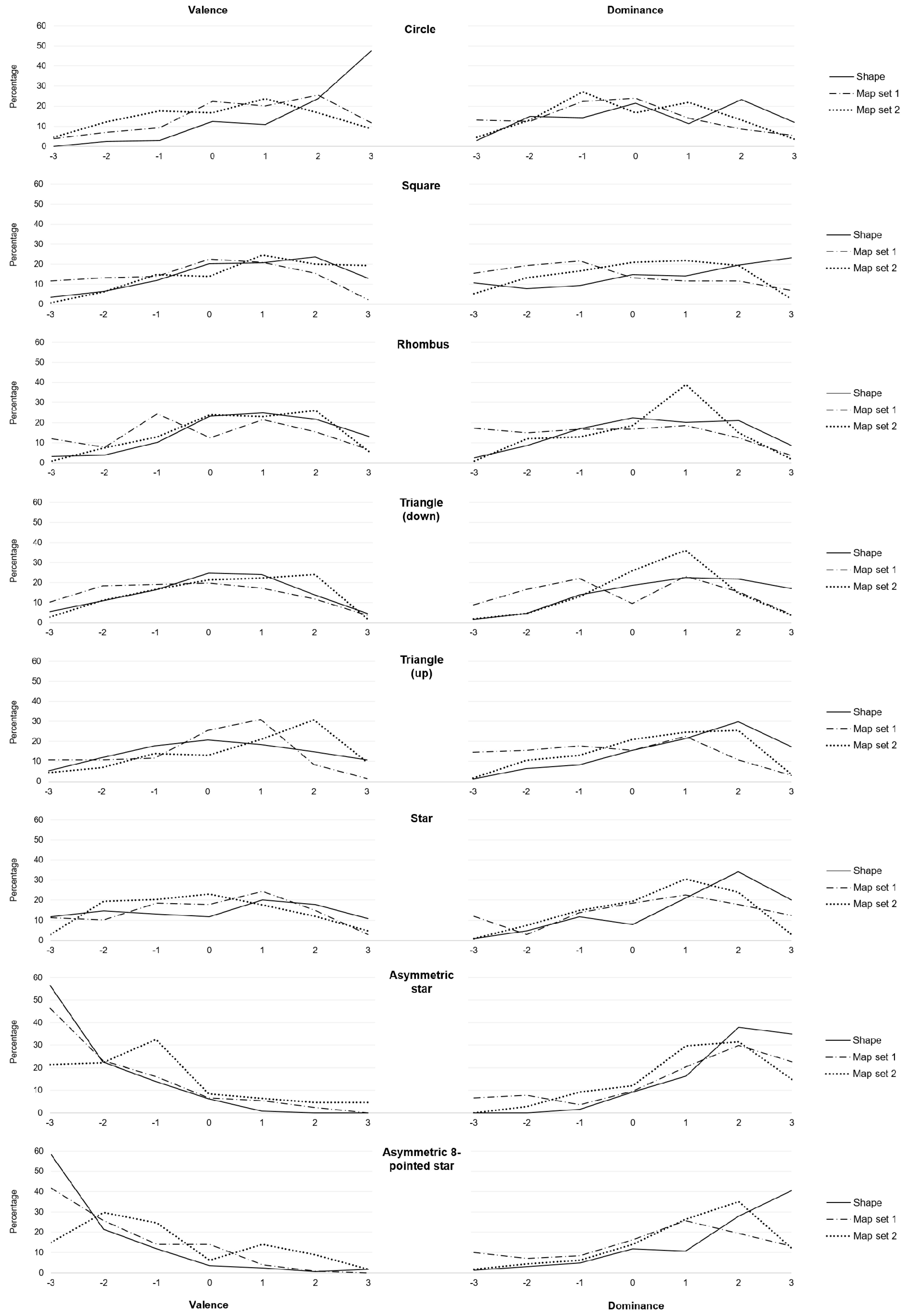
To further explore whether affective shape qualities persisted over the three different stimulus conditions (i.e., with and without cartographic context), the ratings of stimulus-triplets were compared. Stimulus-triplets, here, refer to those three stimuli which depicted the same shape type across the three stimulus conditions. Figure A1 (see Appendix A) contrasts the stimuli’s affective profiles of each stimulus-triplets graphically, concerning their qualities of valence and dominance.
To compare for differences between the stimuli of each triplet, distance scores (D scores) were computed, as suggested by Osgood et al. [16]. Each stimulus-triplet was pairwise compared. A distance measure of D = was applied as proposed by Heise [53], where refers to the mean score of stimulus 1 and to the mean score of stimulus 2 of each stimulus pairing within each triplet. Pairwise comparing the stimuli of each triplet resulted in three D scores for each stimulus-triplet (see Table 5). D scores were computed separately for the two affect dimensions of valence and dominance. Results are summarized in Table 5, revealing detailed distances for each pair in each stimulus-triplet, where higher scores indicate greater dissimilarity and lower scores greater similarities between the stimuli’s affective qualities.
Results show that the star-triplet, in particular, led to the lowest D scores, thus, to highly similar affective ratings on the dimension of valence, in all three stimulus conditions. This finding was also supported by Kruskal–Wallis test for nonparametric data, which found no significant difference between the star stimuli in the three conditions (H(2) = 1.653, p = 0.44). In all other cases, Kruskal–Wallis indicated a statistical significance of p < 0.002 or lower on both affective dimensions of valence and dominance (see Table 5 for detailed distance scores for each stimulus-triplet).
4.4. Multidimensional Scaling
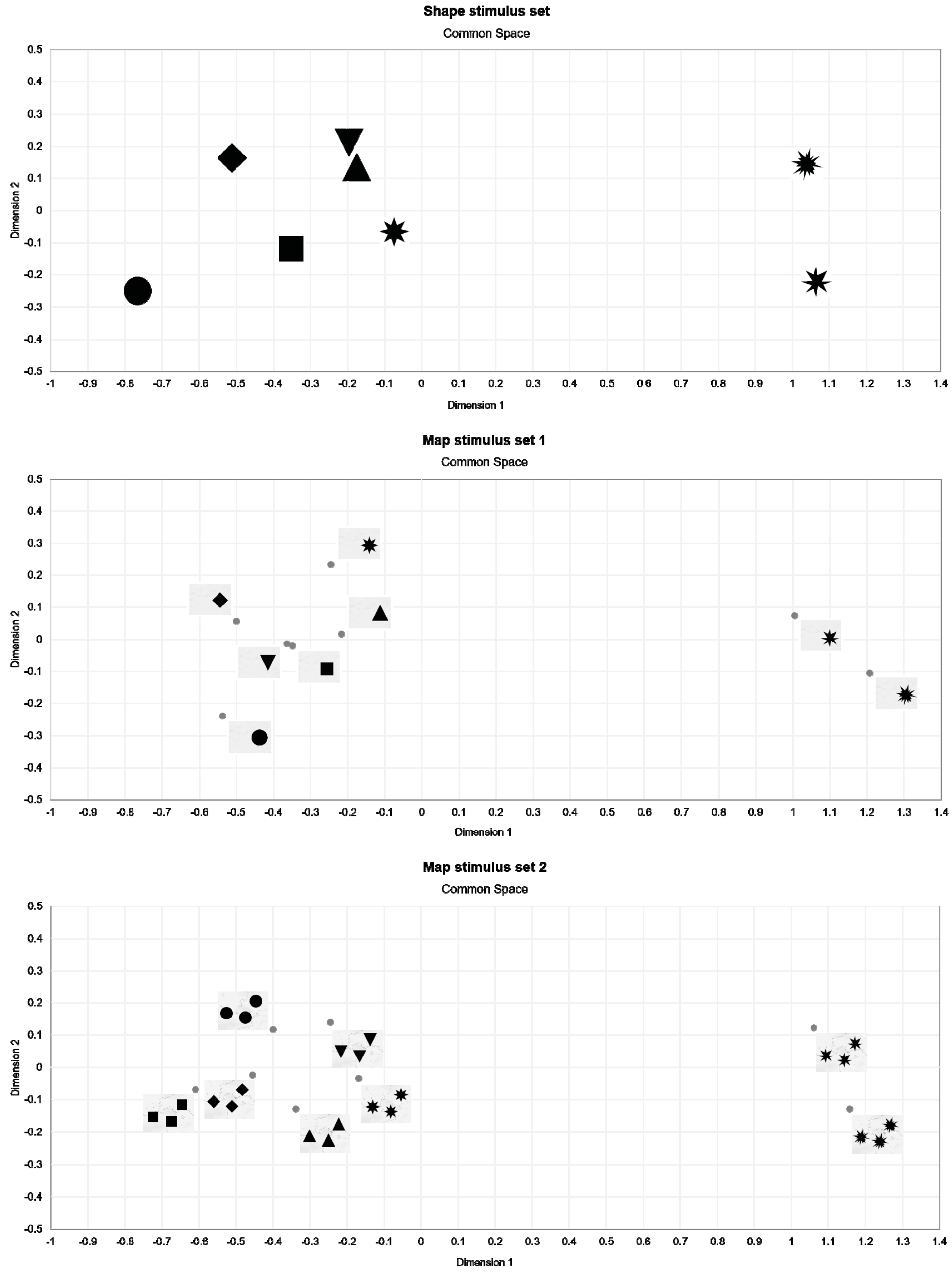
In the final step of the analysis, multidimensional scaling (MDS) was applied to reduce the complexity of the data sets and to permit a visual appreciation of the stimuli’s overall underlying relational structures and proximities. By quantifying distances between stimuli, MDS reveals a dimensional space, wherein similar stimuli are located proximal to each other, and dissimilar ones proportionately farther apart [54]. Thus, for each of the three stimulus conditions, proximities between the individual stimuli were calculated based on the frequency tables composed previously. The frequency tables were subjected to a PROXSCAL scaling algorithm which performs multidimensional scaling of proximity data to find a least-squares representation of objects in a low-dimensional Euclidean space.
Figure 4 visualizes the result, illustrating the relational structure of each stimulus within its stimulus set (see Supplementary Material Table S12 for the coordinates of each stimulus by stimulus set). In the two-dimensional space, revealed similar stimuli were located proximal and dissimilar ones located distant to one another. Between all three stimulus conditions, MDS suggested two distinct stimulus clusters, i.e., one cluster of symmetric stimuli and one cluster of those stimuli depicting asymmetric star shapes. Hence, despite different cartographic and non-cartographic contexts, the overall relational structure between symmetric and asymmetric stimuli was found to prevail.
5. Discussion
As visual means of communication, maps enable us to relate to geospatial phenomena and events from a viewpoint beyond direct experience. As such, maps support us to communicate, to think about, and to imagine the near and the distant. As representations, maps depict and express spatial phenomena but are not the phenomenon itself. Likewise, the visual variables employed in maps, such as map signs and symbols, are abstractions and generalizations, which give rise to an idea or thought of their referents.
While map signs can be considered as identifiers which aim to denote and inform about spatial phenomena, objects, and ideas, related research stresses that signs and symbols imbue connotative qualities which modulate cognitive processes, such as learning, memory, and attention [19,20,28]. Semiotic research in cartography has largely been concerned with the denoting qualities of map signs, by taking into account human perception and cognition to specify characteristics and attributes of visual variables (such as symbols’ size, color hue, etc.). The present research, however, focused on the connotative character of map symbols, by assessing affective qualities of shapes. Eight shape stimuli were presented in three stimulus conditions, i.e., one stimulus set presenting shape stimuli without further context, one stimulus set displaying shapes singularly on a cartographic background, and one stimulus set displaying shapes of the same type on multiple positions on a map. With a semantic differential technique, the affective qualities of the three stimulus sets were assessed and compared within as well as between the three stimulus conditions.
The present study used a deductive approach to decide for the number of affective dimensions and items to employ in a Semantic Differential. Literature indicates two to three affective dimensions, i.e., valence, arousal, and, at times, dominance [16,18,22,23,24,25]. Hence, two bipolar items for each of the three affective dimensions were selected. Based on these questionnaire items, a principal component analysis was conducted to confirm, and respectively reveal, the number of underlying dimensions tested by the Semantic Differential. The principal component analysis extracted two factors. Such a two-factor solution corresponds with the latest affect research, which emphasizes a two-dimensionality of affect [18,28]. In the present study, factor 1 comprised the bipolar items (harmonic, disharmonic; appealing, unappealing; calm, agitated) and factor 2 was composed of the item-pairs (weak, strong; unobtrusive, dominant; passive, dynamic). Hence, based on the bipolar items of each factor, factor 1 was labeled as valence and factor 2 was labeled as dominance. While the extraction of two factors corresponds to the latest theories and findings in affect and emotion research, literature moreover suggests the dimensions of valence and arousal as the two core components of affect. Valence usually refers to evaluative qualities, such as positive, negative, pleasant, unpleasant, appealing, unappealing, etc. Arousal refers to qualities of activation or, respectively, stillness. In the present study, however, the bipolar item calm–agitated loaded high on the dimension of valence, together with the item-pairs harmonic–disharmonic and appealing–unappealing. Given that the present empirical study was conducted in German language, this unexpected item-loading may indicate cross-cultural and linguistic differences. In the German questionnaire, the item-pair calm–agitated translated to “ruhend”– unruhig”. The German term “ruhend” refers to qualities such as dormant, static, and stationary, while the term “unruhig” refers to qualities such as restless, restive, unquiet, and agitated. The findings suggest that the item-pair “ruhend”–“unruhig” may imbue more evaluative valence qualities in German language than their English compounds. This finding, together with results from related affect and emotion research [19,55], may imply the need for more language-sensitive and culture-sensitive approaches in affect research also in the field of cartography.
Based on the two factors extracted, statistical analyses within and between the three stimulus sets were performed. The overall findings strongly suggested two distinct stimuli clusters of particular affective qualities that prevailed over different stimulus conditions, i.e., a cluster of asymmetric stimuli and a cluster of symmetric, geometric stimuli. In each of the three stimulus conditions, those stimuli, which depicted asymmetric stars, scored highly negative on valence (i.e., unappealing, disharmonic, agitated) and highly positive on dominance (i.e., strong, dominant, dynamic). Stimulus material depicting symmetric shapes, on the other hand, overall, scored moderately positive on valence (i.e., appealing, harmonic, calm) and moderately negative in terms of dominance (i.e., weak, unobtrusive, passive). Among the symmetric stimuli, the circular shape, when presented singularly, was further revealed to lead to unique affective responses of high positive valence. Yet, when increasing visual complexity, such as when presenting more than one circular shape on a cartographic background, its distinct positive quality of valence decreased steadily. Such a decrease of affect intensity was also found for most of the stimuli when embedded in visually more complex, cartographic contexts. Only the star stimulus prevailed its affective valence qualities across all three stimulus conditions. In all other cases, the intensity of affect responses decreased on both affective dimensions of valence and dominance when increasing visual complexity, such as when adding a cartographic context or by increasing the number of shape stimuli on a map. This finding strongly implies that cartographic context and visual complexity will influence the degree of affective responses. At this point, it has to be stressed that the cartographic scenarios used in this research referred to simple basemaps in greyscale, yet, free from any further cartographic context, content, or task. Maps can, however, vary greatly in terms of their complexities, due to their sheer unlimited variety of information to depict, visual variables to employ, and contexts in which maps are used. It is, therefore, expected that affective responses will vary in different cartographic settings and scenarios.
Yet, despite the decrease of affect intensity due to context, the affective differentiation between symmetric and asymmetric stimuli appeared to be distinct and to prevail also in the more complex map scenarios of this research study. Empirical research from related fields further supports this notion, suggesting significant preferences for symmetry, even when symmetric shapes are of higher complexity than asymmetric ones [56] or even when shapes are only partially symmetric [57]. Research also shows detection time to be significantly higher in visual search tasks for asymmetric shapes (e.g., elliptic versus circular visual stimuli) [44], again suggesting their unique visual qualities. The present empirical results add to these findings by uncovering particular affective responses towards symmetric and asymmetric shape stimuli which persist in different visual, cartographic contexts.
The overall findings led to the conclusion that shapes imbue qualities which can lead to, at times, highly distinctive affective responses. The asymmetric star stimuli, studied in this research, involved strong and most distinct affective responses, which persisted over different stimulus conditions. Hence, for cartographic communication, the findings strongly imply that asymmetric star shapes may be considered to not only denote but also to connote through qualities of negative valence and positive dominance. Map signs and symbols which are of such qualities can be considered to be more than sheer identifiers. In maps, such shape symbols may, therefore, be employed with particular care, since stimuli with strong expressive, connotative qualities may influence affective responses as well as cognitive processes and related judgments [19,20,28]. Findings from this research further suggest that symmetric shapes, on the other hand, were found to be rather unobtrusive, evoking overall mild affective responses. In a cartographic context, symmetric shape symbols may, therefore, be considered as identifiers to be utilized to depict and denote.
At this point, the findings indicate that relatively simple maps can lead to distinct affective responses. As simple maps have become increasingly prevalent in our daily lives, the results indicate several practical implications. Regularly we encounter web maps in daily routines, such as when reading online news or when orienting or navigating in unfamiliar environments. The web as a new medium constrains the design of maps to the, at times very small, physical display sizes. Well-designed web maps, therefore, require extra attention and are considered as “relatively empty” [58](p. 79). Yet, it remains an open question of how much a simple and relatively empty map can affect how we think about the information depicted, how we imagine a distant event, or how we judge a spatiotemporal phenomenon. How will expressive versus depicting map symbols influence cognitive responses, judgments, memory, and attention in more applied and in different scenarios? Which shape symbols of denoting and expressive character are most suitable for encoding which type of information? Will shape stimuli that are affectively congruent with the information or phenomenon they cartographically depict, amplify judgments of map affect, such as research showed for color congruency [59]? And how do affective responses towards maps and map signs differ by culture, age, and user group? While the present research strongly suggests an influence of map symbols on human affect, future research is needed to tackle these open research questions and to continue exploring the possible impact of putative empty maps and innocent map symbols.
6. Conclusions
Visual communication requires deliberate decisions to share and express information successfully. The choice of the sign-vehicle used to communicate information will affect people’s responses towards the information. While cartographic semiology provides a theoretical framework to communicate geospatial information by addressing the denoting qualities of cartographic visual variables, it does not encompass the connotative qualities of map symbols and their impact on human affect, perception, and cognition. Research from related fields, however, stresses the role of affect as psychologically primitive and as a highly influencing factor on people’s perception, cognition, and behaviors. This research, therefore, aimed to unravel some of the subtle communication effects of shape symbols, by studying the concept of affect in map symbolization.
The present empirical study used a semantic differential technique to assess the affective qualities of shape stimuli in three stimulus conditions of cartographic and non-cartographic context. This research revealed detailed affective profiles for the stimuli studied for both affect dimensions of valence and dominance. The study further identified clusters of stimuli with particular and unique affective qualities. Findings suggest symmetry and asymmetry as crucial factors in how shapes and maps are affectively experienced. Asymmetric stimuli, studied in this research, involved the strongest affective responses, which persisted over both non-cartographic and cartographic stimulus conditions. For cartographic communication, the overall findings led to the conclusion that some shape symbols imbue qualities which can lead to highly distinctive affective responses, and may, therefore, not be considered to be neutral identifiers.
Yet, current findings aim to be expanded upon. Future research is needed to explore the connotative impact of sign-vehicles on more heterogeneous user groups and in different cultures. Research is also needed to further test how the present findings translate to more diverse and applied cartographic contexts, such as when depicting different types of geospatial information or when increasing the level of visual complexity. With a profound understanding of the subtle communication qualities of cartographic sign-vehicles and their effects on human responses, graphic variables can be more accurately discriminated, leading to more informed decisions in the process of cartographic communication.
Supplementary Materials
The following are available online at https://0-www-mdpi-com.brum.beds.ac.uk/2220-9964/9/5/289/s1. Table S1. PCA: Total variance explained. Table S2. PCA: Rotated component matrix. Figure S1. PCA: Component plot. Table S3. Shape stimulus set: Descriptive statistics. Table S4. Map stimulus set 1: Descriptive statistics. Table S5. Map stimulus set 2: Descriptive statistics. Table S6. Shape stimulus set: Frequencies of affective shape ratings. Table S7. Map stimulus set 1: Frequencies of affective shape ratings. Table S8. Map stimulus set 2: Frequencies of affective shape ratings. Table S9. Shape stimulus set: Conover–Iman pairwise stimulus comparisons. Table S10. Map stimulus set 1: Conover–Iman pairwise stimulus comparisons. Table S11. Map stimulus set 2: Conover–Iman pairwise stimulus comparisons. Table S12. MDS-based coordinates by shape and stimulus set.
Funding
This research received no external funding.
Acknowledgments
The author thanks Georg Gartner for his valuable feedback and support in this research. The author thanks the three anonymous reviewers for their comments and suggestions. The author further thanks the academic editors of this journal for the opportunity to share this research. The author acknowledges TU Wien University Library for financial support through its Open Access Funding Program.
Conflicts of Interest
The author declares no conflict of interest.
Appendix A
Figure A1.
Affective responses towards eight shape stimuli compared between the three stimulus conditions by valence (left) and dominance (right).
Figure A1.
Affective responses towards eight shape stimuli compared between the three stimulus conditions by valence (left) and dominance (right).
References
- Krauss, R.M. The Psychology of Verbal Communication. In International Encyclopedia of the Social and Behavioral Sciences; Smelser, N.J., Baltes, P., Eds.; Elsevier: Amsterdam, The Netherlands, 2002. [Google Scholar]
- Howard, V.A. Theory of representation: Three questions. In Processing of Visible Language; Springer US: Boston, MA, USA, 1980; pp. 501–515. [Google Scholar]
- Petchenik, B. Cognition in Cartography. Cartogr. Int. J. Geogr. Inf. Geovisualization 1977, 14, 117–128. [Google Scholar] [CrossRef] [Green Version]
- Eide, Ø. Media Boundaries and Conceptual Modelling: Between Texts and Maps; Palgrave Macmillan: London, UK, 2016; ISBN 978-1349566235. [Google Scholar]
- Harley, J.B. Maps, knowledge, and power. In Geographic Thought: A Praxis Perspective; Henderson, G., Waterstone, M., Eds.; Routledge: Abingdon-on-Thames, UK, 2009. [Google Scholar]
- Wood, D. Rethinking the Power of Maps; The Guilford Press: New York, NY, USA, 2010. [Google Scholar]
- Thompson, M.A.; Lindsay, J.M.; Gaillard, J. The influence of Probabilistic Volcanic Hazard map Properties on Hazard Communication. J. Appl. Volcanol. 2011, 4, 6. [Google Scholar] [CrossRef] [Green Version]
- Monmonier, M. How to Lie with Maps; The University of Chicago Press: Chicago, IL, USA, 1996. [Google Scholar]
- Bertin, J. Graphische Semiologie: Diagramme, Netze, Karten; Walter de Gruyter: Berlin, Germany, 1974. [Google Scholar]
- Klee, P. Schöpferische Konfession: Paul Klee. In Tribüne der Kunst und Zeit—Eine Schriftensammlung, Band XIII; Edschmid, K., Ed.; Erich Reiß Verlag: Berlin, Germany, 1920; pp. 28–40. [Google Scholar]
- Arnheim, R. Art and Visual Perception: A Psychology of the Creative Eye; University of California Press: Berkeley, CA, USA, 1974; ISBN 0520243838. [Google Scholar]
- Nöth, W. Handbook of Semiotics; Indiana University Press: Blomington, IN, USA, 1995; ISBN 978-0-253-20959-7. [Google Scholar]
- Morris, C.W. Foundations of the Theory of Signs; The University of Chicago Press: Chicago, IL, USA, 1938; pp. 1–59. [Google Scholar]
- Morris, C.W. Signs, Language And Behavior, 1st ed.; George Braziller, Inc.: New York, NY, USA, 1946. [Google Scholar]
- MacEachren, A.M. How Maps Work: Representation, Visualization, and Design; The Guilford Press: New York, NY, USA, 1995; ISBN 0-89862-589-0. [Google Scholar]
- Osgood, C.E.; Suci, G.J.; Tannenbaum, P.H. The Measurement of Meaning; University of Illinois Press: Urbana, IL, USA, 1967. [Google Scholar]
- Keates, J.S. Understanding Maps, 2nd ed.; Addison Wesley Longman Limited: New York, NY, USA, 1996. [Google Scholar]
- Barrett, L.F.; Bliss-Moreau, E. Affect as a Psychological Primitive. Adv. Exp. Soc. Psychol. 2009, 41, 167–218. [Google Scholar]
- Sianipar, A.; Van Groenestijn, P.; Dijkstra, T. Affective Meaning, Concreteness, and Subjective Frequency Norms for Indonesian Words. Front. Psychol. 2016, 7, 1907. [Google Scholar] [CrossRef] [Green Version]
- Loftus, E.F.; Palmer, J.C. Reconstruction of Automobile Deconstruction: An Example of the Interaction Between Language and Memory. J. Verbal Learn. Verbal Behav. 1974, 13, 585–589. [Google Scholar] [CrossRef]
- Osgood, C.E.; Luria, Z. A blind analysis of a case of multiple personality using the Semantic Differnetial. J. Abnorm. Soc. Psychol. 1954, 49, 579–591. [Google Scholar] [CrossRef]
- Mehrabian, A.; Russell, J.A. An Approach to Environmental Psychology; The Massachusetts Institute of Technology: Cambridge, MA, USA, 1974. [Google Scholar]
- Espe, H. A cross-cultural investigation of the graphic differential. J. Psycholinguist. Res. 1985, 14, 97–111. [Google Scholar] [CrossRef]
- Bakker, I.; Van Der Voordt, T.; Vink, P.; De Boon, J. Pleasure, arousal, dominance: Mehrabian and Russell revisited. Curr. Psychol. 2014, 33, 405–421. [Google Scholar] [CrossRef]
- Russell, J.A. A Circumplex Model of Affect. J. Pers. Soc. Psychol. 1980, 39, 1161–1178. [Google Scholar] [CrossRef]
- Wunth, W. Grundriss der Psychologie, 5th ed.; Wilhelm Engelmann: Leipzig, Germany, 1902. [Google Scholar]
- Russell, J.A. Core Affect and the Psychological Construction of Emotion. Psychol. Rev. 2003, 110, 145–172. [Google Scholar] [CrossRef]
- Feldman Barrett, L.; Mesquita, B.; Ochsner, K.N.; Gross, J.J. The Experience of Emotion. Annu. Rev. Psychol. 2007, 58, 373–403. [Google Scholar] [CrossRef] [Green Version]
- Griffin, A.L.; McQuoid, J. At the Intersection of Maps and Emotion: The Challenge of Spatially Representing Experience. Kartogr. Nachr. 2012, 6, 291–299. [Google Scholar]
- Nold, C. Emotional Cartography: Technologies of the Self; Space Studios: London, UK, 2009. [Google Scholar]
- Klettner, S.; Huang, H.; Schmidt, M.; Gartner, G. Crowdsourcing affective responses to space. J. Cartogr. Geogr. Inf. 2013, 2, 66–72. [Google Scholar]
- Fabrikant, S.I.; Christophe, S.; Papastefanou, G.; Maggi, S. Emotional Response to Map Design Aesthetics. In Proceedings of the 7th International Conference on Geographical Information Science, Columbus, OH, USA, 18–21 September 2012. [Google Scholar]
- Christophe, S.; Hoarau, C. Expressive Map Design Based on Pop Art: Revisit of Semiology of Graphics? Cartogr. Perspect. 2013, 61–74. [Google Scholar] [CrossRef] [Green Version]
- Muehlenhaus, I. If Looks Could Kill: The Impact of Different Rhetorical Styles on Persuasive Geocommunication. Cartogr. J. 2012, 49, 361–375. [Google Scholar] [CrossRef]
- Muehlenhaus, I. The Design and Composition of Persuasive Maps. Cartogr. Geogr. Inf. Sci. 2013, 40, 404–414. [Google Scholar] [CrossRef]
- Jenny, B.; Stephen, D.M.; Muehlenhaus, I.; Marston, B.E.; Sharma, R.; Zhang, E.; Jenny, H. Design Principles for Origin-destination Flow Maps. Cartogr. Geogr. Inf. Sci. 2018, 45, 62–75. [Google Scholar] [CrossRef]
- Stachoň, Z.; Šašinka, Č.; Čeněk, J.; Angsüsser, S.; Kubíček, P.; Štěrba, Z.; Bilíková, M. Effect of Size, Shape and Map Background in Cartographic Visualization: Experimental Study on Czech and Chinese Populations. ISPRS Int. J. Geo-Inf. 2018, 7, 427. [Google Scholar] [CrossRef] [Green Version]
- MacEachren, A.M.; Roth, R.E.; O’Brien, J.; Li, B.; Swingley, D.; Gahegan, M. Visual Semiotics and Uncertainty Visualization: An Empirical Study. IEEE Trans. Vis. Comput. Graph. 2012, 18, 2496–2505. [Google Scholar] [CrossRef]
- Padilla, L.M.; Ruginski, I.T.; Creem-Regehr, S.H. Effects of ensemble and summary displays on interpretations of geospatial uncertainty data. Cogn. Res. Princ. Implic. 2017, 2, 40. [Google Scholar] [CrossRef] [Green Version]
- Kinkeldey, C.; MacEachren, A.M.; Schiewe, J. How to Assess Visual Communication of Uncertainty? A Systematic Review of Geospatial Uncertainty Visualisation User Studies. Cartogr. J. 2014, 51, 372–386. [Google Scholar] [CrossRef]
- Cheong, L.; Bleisch, S.; Kealy, A.; Tolhurst, K.; Wilkening, T.; Duckham, M. Evaluating the impact of visualization of wildfire hazard upon decision-making under uncertainty. Int. J. Geogr. Inf. Sci. 2016, 30, 1377–1404. [Google Scholar] [CrossRef] [Green Version]
- Chandler, D. Semiotics: The Basics; Routledge: Abingdon-on-Thames, UK, 2007. [Google Scholar]
- Arnheim, R. Kunst Und Sehen: Eine Psychologie des Schöpferischen Auges; Walter de Gruyter: Berlin, Germany, 1978; ISBN 3110066823. [Google Scholar]
- Treisman, A.; Gormican, S. Feature Analysis in Early Vision: Evidence From Search Asymmetries. Psychol. Rev. 1988, 95, 15. [Google Scholar] [CrossRef]
- Limesurvey GmbH. LimeSurvey: An Open Source Survey Tool; LimeSurvey GmbH: Hamburg, Germany, 2019. [Google Scholar]
- Russell, J.A.; Pratt, G. A Description of the Affective Quality Attributed to Environments. J. Pers. Soc. Psychol. 1980, 38, 311–322. [Google Scholar] [CrossRef]
- Klettner, S. Why Shape Matters—On the Inherent Qualities of Geometric Shapes for Cartographic Representations. ISPRS Int. J. Geo-Inf. 2019, 8, 217. [Google Scholar] [CrossRef] [Green Version]
- IBM Corp. IBM SPSS Statistics for Windows; Version 25.0; IBM Corp: Armonk, NY, USA, 2017. [Google Scholar]
- Addinsoft XLSTAT 2020; Addinsoft: New York, NY, USA, 2020.
- Field, A. Discovering Statistics Using IBM SPSS Statistics, 3rd ed.; SAGE Publications Ltd: Thousand Oaks, CA, USA, 2009. [Google Scholar]
- Chatfield, M.; Mander, A. The Skillings-Mack test (Friedman test when there are missing data). Stata J. 2009, 9, 299–305. [Google Scholar] [CrossRef] [PubMed]
- Conover, W.J.; Iman, R.L. On Multiple-Comparisons Procedures; Los Alamos National Lab: Los Alamos, NM, USA, 1979. [Google Scholar]
- Heise, D.R. The Semantic Differential and Attitude Research. Attitude Meas. 1970, 4, 235–253. [Google Scholar]
- Hout, M.C.; Papesh, M.H.; Goldinger, S.D. Multidimensional Scaling. Wiley Interdiscip. Rev. Cogn. Sci. 2013, 4, 93–103. [Google Scholar] [CrossRef]
- Russell, J.A.; Lewicka, M.; Niit, T. A Cross-Cultural Study of a Circumplex Model of Affect. J. Pers. Soc. Psychol. 1989, 57, 848–856. [Google Scholar] [CrossRef]
- Eisenman, R.; Rappaport, J. Complexity preference and semantic differential ratings of complexity-simplicity and symmetry-asymmetry. Psychon. Sci. 1967, 7, 147–148. [Google Scholar] [CrossRef]
- Friedenberg, J.; Bertamini, M. Aesthetic Preference for Polygon Shape Contour Variation and Perceived Beauty of Polygon Shape Polygons and Art. Empir. Stud. Arts 2015, 33, 144–160. [Google Scholar] [CrossRef]
- Kraak, M.J.; Ormeling, F. Cartography: Visualization of Spatial Data; Guilford Press: New York, NY, USA, 2011; ISBN 9781609181932. [Google Scholar]
- Anderson, C. The Influence of Affectively Congruent Color Assignment in Categorical Map; Penn State University: State College, PA, USA, 2018. [Google Scholar]
Figure 1.
Illustration of the triadic sign relation, known as the semiotic triangle, considering (a) the interpretant as mediator, (b) the referent as mediator, and (c) the sign-vehicle as mediator [12,15].
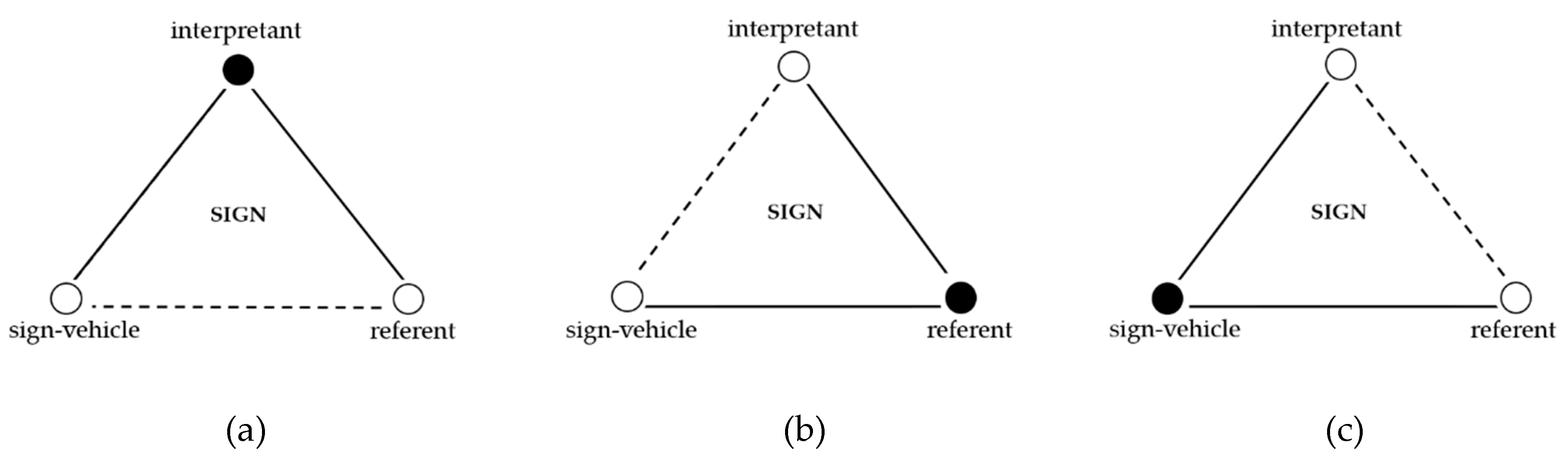
Figure 2.
Between-subjects design applied for three stimulus sets. Screenshots of the survey are shown to the left, illustrating the stimulus materials as used in the surveys. Shape and map stimuli used in the study are illustrated to the right, according to the two between-subjects stimulus groups (A and B). Note that map symbols depicted to the right are highly enlarged to enhance legibility.
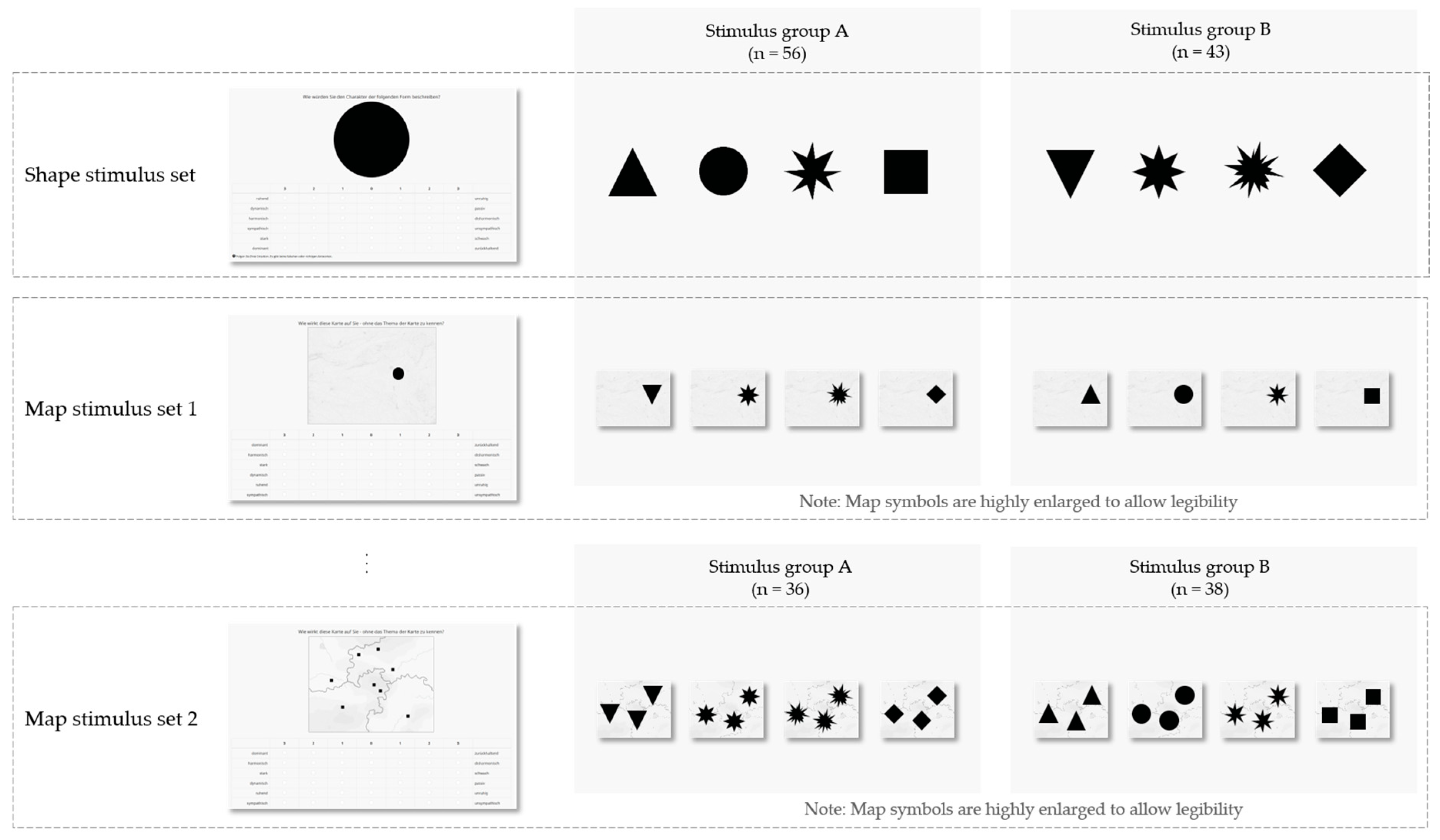
Figure 3.
Affective quality ratings of valence (left) and dominance (right) of eight stimuli in three stimulus conditions.
Figure 3.
Affective quality ratings of valence (left) and dominance (right) of eight stimuli in three stimulus conditions.
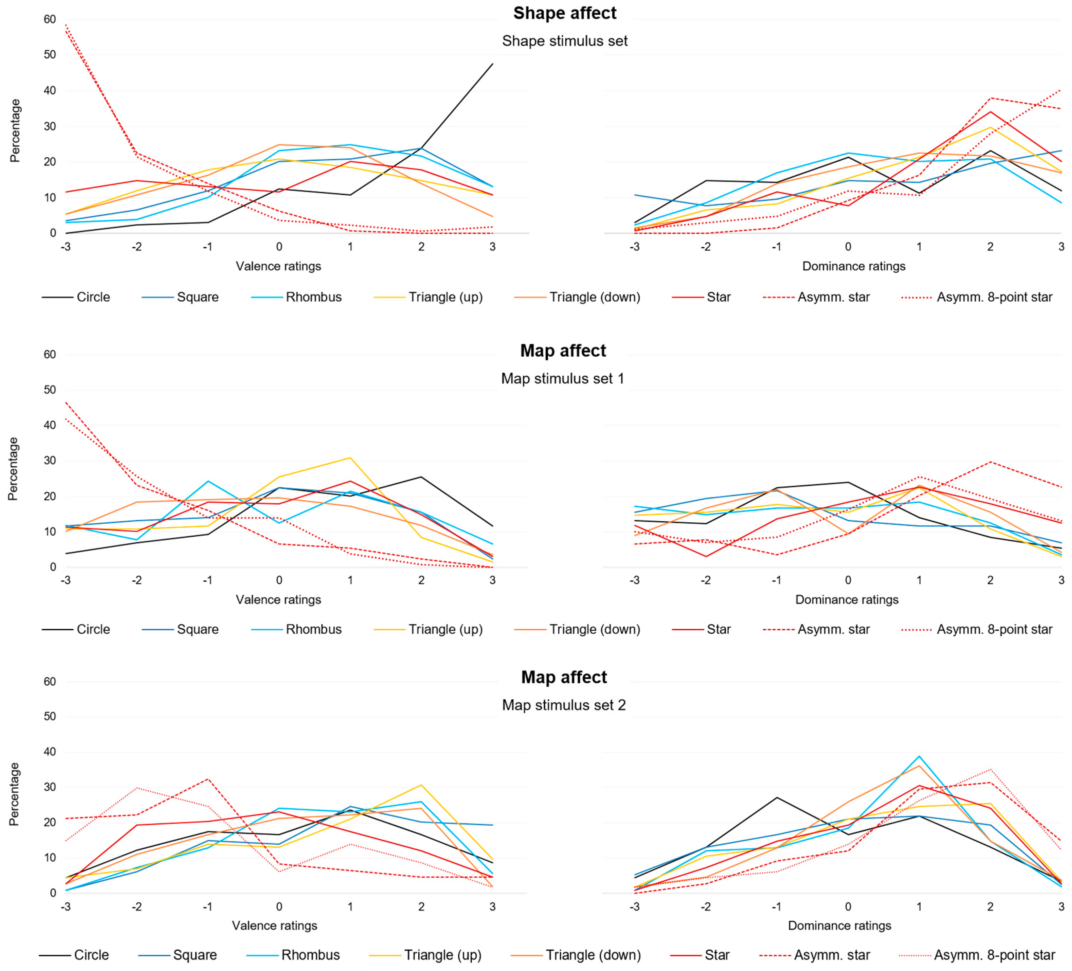
Figure 4.
Two-dimensional configuration based on multidimensional scaling, indicating the proximities between the eight stimuli within each stimulus set.
Figure 4.
Two-dimensional configuration based on multidimensional scaling, indicating the proximities between the eight stimuli within each stimulus set.


Table 1.
Semantic differential items used in the present study in German and translated into English.
Table 1.
Semantic differential items used in the present study in German and translated into English.
| Bipolar Items | Bipolar Items in German (Original) |
|---|---|
| unappealing – appealing | unsympatisch – sympathisch |
| disharmonic – harmonic | disharmonisch – harmonisch |
| unobtrusive – dominant | zurückhaltend – dominant |
| weak – strong | schwach – stark |
| calm – agitated | ruhend – unruhig |
| passive – dynamic | passiv – dynamisch |
Table 2.
Results of multiple pairwise comparisons of shape stimuli indicating groups of similar valence and dominance.
Table 2.
Results of multiple pairwise comparisons of shape stimuli indicating groups of similar valence and dominance.
| Stimulus | Frequency | Sum of ranks | Mean of ranks | Groups (Valence) | ||||
| Circle | 168 | 155604.50 | 926.22 |  A A | ||||
| Rhombus | 129 | 94532.50 | 732.81 |  B B | ||||
| Square | 168 | 120860.00 | 719.40 |  B B | C | |||
| Triangle (up) | 168 | 106916.00 | 636.40 |  C C | D | |||
| Star | 129 | 79942.50 | 619.71 |  D D | ||||
| Triangle (down) | 129 | 79567.50 | 616.80 |  D D | ||||
| Asymm. 8-point star | 168 | 39855.50 | 237.24 |  E E | ||||
| Asymm. star | 129 | 28987.50 | 224.71 |  E E | ||||
| Stimulus | Frequency | Sum of ranks | Mean of ranks | Groups (Dominance) | ||||
| Asymm. 8-point star | 129 | 100290.00 | 777.44 | A | ||||
| Asymm. star | 168 | 125539.00 | 747.26 | A | B | |||
| Star | 129 | 81415.50 | 631.13 | B | C | |||
| Triangle (up) | 168 | 99149.50 | 590.18 | C | ||||
| Triangle (down) | 129 | 70898.50 | 549.60 | C | D | |||
| Square | 168 | 90942.00 | 541.32 | C | D | |||
| Circle | 168 | 78421.50 | 466.79 | D | ||||
| Rhombus | 129 | 59610.00 | 462.09 | D | ||||
Table 3.
Results of multiple pairwise comparisons of map stimulus set 1 indicating groups of similar valence and dominance.
Table 3.
Results of multiple pairwise comparisons of map stimulus set 1 indicating groups of similar valence and dominance.
| Stimulus | Frequency | Sum of ranks | Mean of ranks | Groups (Valence) | |||
| Circle | 129 | 105739.00 | 819.68 |  A A | |||
| Rhombus | 168 | 114192.50 | 679.72 |  B B | |||
| Star | 168 | 113034.00 | 672.82 |  B B | |||
| Triangle (up) | 129 | 86270.50 | 668.76 |  B B | |||
| Square | 129 | 85176.50 | 660.28 |  B B | |||
| Triangle (down) | 168 | 104689.00 | 623.15 |  B B | |||
| Asymm. 8-point star | 129 | 43106.50 | 334.16 |  C C | |||
| Asymm. star | 168 | 54058.00 | 321.77 |  C C | |||
| Stimulus | Frequency | Sum of ranks | Mean of ranks | Groups (Dominance) | |||
| Asymm. star | 168 | 133241.50 | 793.10 | A | |||
| Asymm. 8-point star | 129 | 88048.50 | 682.55 | A | B | ||
| Star | 168 | 111135.50 | 661.52 | B | C | ||
| Triangle (down) | 168 | 93561.50 | 556.91 | C | D | ||
| Triangle (up) | 129 | 66187.50 | 513.08 | D | |||
| Circle | 129 | 65608.50 | 508.59 | D | |||
| Rhombus | 168 | 85052.00 | 506.26 | D | |||
| Square | 129 | 63431.00 | 491.71 | D | |||
Note: Map symbols are depicted highly enlarged to allow legibility.
Table 4.
Results of multiple pairwise comparisons of map stimulus set 2 indicating groups of similar valence and dominance.
Table 4.
Results of multiple pairwise comparisons of map stimulus set 2 indicating groups of similar valence and dominance.
| Stimulus | Frequency | Sum of ranks | Mean of ranks | Groups (Valence) | ||
| Square | 114 | 64620.50 | 566.85 |  A A | ||
| Triangle (up) | 114 | 61362.00 | 538.26 |  A A | ||
| Rhombus | 108 | 56467.00 | 522.84 |  A A | ||
| Triangle (down) | 108 | 51321.00 | 475.19 |  A A | B | |
| Circle | 114 | 53840.50 | 472.29 |  A A | B | |
| Star | 108 | 44328.00 | 410.44 |  B B | ||
| Asymm. 8-point star | 114 | 33732.00 | 295.89 |  C C | ||
| Asymm. star | 108 | 29045.00 | 268.94 |  C C | ||
| Stimulus | Frequency | Sum of ranks | Mean of ranks | Groups (Dominance) | ||
| Asymm. star | 108 | 61100.50 | 565.75 | A | ||
| Asymm. 8-point star | 114 | 63355.00 | 555.75 | A | ||
| Star | 108 | 48153.00 | 445.86 | B | ||
| Triangle (up) | 114 | 49661.00 | 435.62 | B | C | |
| Triangle (down) | 108 | 46351.00 | 429.18 | B | C | |
| Rhombus | 108 | 44182.50 | 409.10 | B | C | |
| Square | 114 | 42927.00 | 376.55 | B | C | |
| Circle | 114 | 38986.00 | 341.98 | C | ||
Note: Map symbols are depicted highly enlarged to allow legibility.
Table 5.
Distance scores of each stimulus-triplet pairwise compared. Lower scores indicate lower distance, i.e., greater similarity (see lighter cell colors). Higher scores indicate greater dissimilarity (see darker cell colors).
Table 5.
Distance scores of each stimulus-triplet pairwise compared. Lower scores indicate lower distance, i.e., greater similarity (see lighter cell colors). Higher scores indicate greater dissimilarity (see darker cell colors).
| Triangle (up) | Triangle (down) | Circle | Star | Square | Rhomb | Asymm. star | Asymm. 8-pt star | |
|---|---|---|---|---|---|---|---|---|
| Valence: | ||||||||
| Shape – Map ss | 0.36 | 0.46 | 1.22 | 0.20 | 0.88 | 0.84 | 0.36 | 0.36 |
| Map ss – Map ms | 0.83 | 0.63 | 0.43 | 0.03 | 1.09 | 0.65 | 0.81 | 0.93 |
| Map ms – Shape | 0.48 | 0.17 | 1.65 | 0.23 | 0.21 | 0.20 | 1.17 | 1.29 |
| Dominance: | ||||||||
| Shape – Map ss | 1.47 | 1.05 | 0.80 | 0.86 | 1.17 | 0.91 | 0.86 | 1.23 |
| Map ss – Map ms | 0.86 | 0.65 | 0.32 | 0.14 | 0.61 | 0.78 | 0.13 | 0.62 |
| Map ms – Shape | 0.61 | 0.40 | 0.48 | 0.72 | 0.56 | 0.12 | 0.73 | 0.61 |
Note: “Shape” refers to stimuli from the shape stimulus set, “Maps ss” refers to stimuli from map stimulus set 1 (i.e., maps depicting a single shape), and “Maps ms” refers to stimuli from map stimulus set 2 (i.e., maps depicting multiple shapes).
© 2020 by the author. Licensee MDPI, Basel, Switzerland. This article is an open access article distributed under the terms and conditions of the Creative Commons Attribution (CC BY) license (http://creativecommons.org/licenses/by/4.0/).
Share and Cite
MDPI and ACS Style
Klettner, S. Affective Communication of Map Symbols: A Semantic Differential Analysis. ISPRS Int. J. Geo-Inf. 2020, 9, 289. https://0-doi-org.brum.beds.ac.uk/10.3390/ijgi9050289
AMA Style
Klettner S. Affective Communication of Map Symbols: A Semantic Differential Analysis. ISPRS International Journal of Geo-Information. 2020; 9(5):289. https://0-doi-org.brum.beds.ac.uk/10.3390/ijgi9050289
Chicago/Turabian StyleKlettner, Silvia. 2020. "Affective Communication of Map Symbols: A Semantic Differential Analysis" ISPRS International Journal of Geo-Information 9, no. 5: 289. https://0-doi-org.brum.beds.ac.uk/10.3390/ijgi9050289
Note that from the first issue of 2016, this journal uses article numbers instead of page numbers. See further details here.