Towards Automatic Points of Interest Matching


Department of Computer Science, AGH University of Science and Technology, al. Mickiewicza 30, 30-059 Krakow, Poland
*
Author to whom correspondence should be addressed.
ISPRS Int. J. Geo-Inf. 2020, 9(5), 291; https://0-doi-org.brum.beds.ac.uk/10.3390/ijgi9050291
Submission received: 31 March 2020
/
Revised: 16 April 2020
/
Accepted: 22 April 2020
/
Published: 1 May 2020
Abstract
:Complementing information about particular points, places, or institutions, i.e., so-called Points of Interest (POIs) can be achieved by matching data from the growing number of geospatial databases; these include Foursquare, OpenStreetMap, Yelp, and Facebook Places. Doing this potentially allows for the acquisition of more accurate and more complete information about POIs than would be possible by merely extracting the information from each of the systems alone. Problem: The task of Points of Interest matching, and the development of an algorithm to perform this automatically, are quite challenging problems due to the prevalence of different data structures, data incompleteness, conflicting information, naming differences, data inaccuracy, and cultural and language differences; in short, the difficulties experienced in the process of obtaining (complementary) information about the POI from different sources are due, in part, to the lack of standardization among Points of Interest descriptions; a further difficulty stems from the vast and rapidly growing amount of data to be assessed on each occasion. Research design and contributions: To propose an efficient algorithm for automatic Points of Interest matching, we: (1) analyzed available data sources—their structures, models, attributes, number of objects, the quality of data (number of missing attributes), etc.—and defined a unified POI model; (2) prepared a fairly large experimental dataset consisting of 50,000 matching and 50,000 non-matching points, taken from different geographical, cultural, and language areas; (3) comprehensively reviewed metrics that can be used for assessing the similarity between Points of Interest; (4) proposed and verified different strategies for dealing with missing or incomplete attributes; (5) reviewed and analyzed six different classifiers for Points of Interest matching, conducting experiments and follow-up comparisons to determine the most effective combination of similarity metric, strategy for dealing with missing data, and POIs matching classifier; and (6) presented an algorithm for automatic Points of Interest matching, detailing its accuracy and carrying out a complexity analysis. Results and conclusions: The main results of the research are: (1) comprehensive experimental verification and numerical comparisons of the crucial Points of Interest matching components (similarity metrics, approaches for dealing with missing data, and classifiers), indicating that the best Points of Interest matching classifier is a combination of random forest algorithm coupled with marking of missing data and mixing different similarity metrics for different POI attributes; and (2) an efficient greedy algorithm for automatic POI matching. At a cost of just 3.5% in terms of accuracy, it allows for reducing POI matching time complexity by two orders of magnitude in comparison to the exact algorithm.
1. Introduction
The rising popularity and accessibility of devices with a GPS receiver has had an impact on the growth of geospatial databases. Spatial data are utilized in many mobile and web applications, such as augmented reality games, e.g., Pokémon GO (https://www.pokemongo.com/) or Geocaching (https://www.geocaching.com/); social media applications, which allow for the exchange of the current locations of the users by “checking in” to places where they spend time; social utility applications, such as FixMyStreet (www.fixmystreet.com) and The Water Project (https://thewaterproject.org/), which allow a user to submit data regarding places that require the attention of a local authority or a charity; and genuine databases such as OpenStreetMap (https://www.openstreetmap.org/) or DBpedia (https://wiki.dbpedia.org/) created to collect various pieces of information about many geographical objects. Unfortunately, the fact that there is a growing number of diverse (geospatial) databases, powered by data from thousands of users, does not necessarily mean that we can automatically and easily compare and combine data concerning the interesting points or places, so-called Points of Interest (POIs), in order to obtain a complete set of information about the given POI. The reasons for this include, among others: different data structures in particular databases, data incompleteness, conflicting information, naming differences, data inaccuracy, and cultural and language differences. In other words, we are confronted by a lack of standardization with regards to the Points of Interest descriptions. The problem is further compounded by the huge, and fast-growing, amount of data to be assessed every time (complementary) information is sought about a POI via these diverse sources.
Figure 1 shows data models used to store information about POIs by four popular data sources. It gives a general overview of the issues involved when combining information about the same Point of Interest from different databases. Due to the limited space available, the figure presents only fragments of data models. Nevertheless, even for the few popular attributes presented, one may see how significant the differences between them all are. For instance, the attribute name is a top-level attribute in Foursquare, Yelp, and Facebook Places models, but, in the OpenStreetMap model, it is one of the (optional) tags. The geographical location attribute is sometimes a “location” complex attribute with nested “lat” and “lng” (sub)attributes as in the Foursquare model, while, other times, it is a “coordinates” complex attribute with nested “latitude” and “longitude” (sub)attributes; on yet other occasions, location is represented as a top-level “lat” and “lon” pair of attributes as in the OpenStreetMap model. Similar differences can be seen, for instance, for information representing phone number, category, website, etc. The second serious problem is the incompleteness of the information, not to mention the discrepancies, errors, and ambiguities in the data itself. Examples of these problems are:
- The manner in which numbers are presented, e.g., Restaurant Paracas II in OpenStreetMap versus Paracas 2 in Yelp;
- Attribute value incompleteness, e.g., Daddy’s in Foursquare versus Daddy’s Pizza& Billiard in Yelp;
- Language differences, e.g., Doutor Coffee Shop in Foursquare versus ドトールコーヒーショップ in Yelp;
- Text formatting differences (blank spaces, word order, etc.), e.g., Caleta Rosa in Foursquare versus RosaCaleta in Yelp;
- Phone number formatting differences, e.g., 2129976801 in Foursquare versus +12129976801 in OpenStreetMap;
- URL format differences, e.g., http://www.juicepress.com in Foursquare versus https://juicepress.com in OpenStreetMap;
- Category distinctions: for instance, in OpenStreetMap an in-depth analysis of the object’s attributes is required to find and anticipate which attributes might point to the category (e.g., amenity, tourism, keys with a value of “yes” etc.);
- Differences in geographical coordinates (as outlined in Section 4.1.1), which are so significant that the search radius, within which matching points in other data sources might be obtained, should be as long as 300 m to have sufficient confidence of finding a matching POI, if there is one;
- Data incompleteness, i.e., a significant proportion of attributes for a given Point of Interest have empty values. Moreover, one part of data may be completed for a given point in one source and another part in another source. Naturally, it would be advantageous to simply assemble data which are “scattered” across various sources in the hope that we acquire a range of diverse (complementary) data points. Given this aim, in a certain sense, it is extremely helpful that there are different pieces of data arising from these various sources. However, when we wish to determine whether the analyzed POI refers to the same real place, then suddenly the task becomes rather problematic. The reason for this is that there is a scarcity of “common data” on the basis of which the POIs can be identified and classified as matching. For instance, one very distinctive attribute, namely the www address, cannot be used as a basis for identifying matching points since in Yelp the value for this attribute has been provided for 0% of Points of Interest. A broader and more detailed analysis of this problem for our 100,000-point training set, broken down into individual data sources and attributes, is given in Section 3.2.
Therefore, the problem of pinpointing entries referring to the same real-world entities in the geospatial databases is an important and challenging area of research. Despite the fact that the issue is preliminarily addressed in the literature, it is still difficult to deduce which approach is the most appropriate. One reason for this, is that in the published research (described in Section 2), experiments have been carried out on very small datasets. In addition, there is no comprehensive analysis of the different similarity metrics, classification algorithms, and approaches to incomplete data with regards to POI matching. Furthermore, the partial research that has been done so far was carried out on disjunctive sets of data, making it difficult to draw any clear comparisons and conclusions.
In this paper, to address the problems identified and conclude with an automatic algorithm for POIs matching, a two-stage research procedure is reported.
The first stage is focused on a comprehensive survey of the crucial aspects of the Points of Interest matching process and elements, namely:
- the size and diversity of the datasets and the data sources;
- the metrics used to assess the similarity of the Points of Interest;
- the missing values of attributes employed by the matching algorithms; and
- the classification algorithms used to match the objects.
This survey and in-depth analysis allowed us to put forward, in the second stage, an algorithm for the automatic matching of spatial objects sourced from different databases.
The remainder of the paper is organized as follows:
- In Section 2, the work related to POIs matching done thus far is briefly reviewed.
- In Section 3, the data sources, the unification of Points of Interest models and the preparation of experimental datasets are discussed.
- In Section 4, three crucial elements of Points of Interest matching classifiers, namely similarity metrics (see Section 4.1), strategies for dealing with missing data (see Section 4.2), and classification algorithms (see Section 4.3), are discussed.
- In Section 5, the results of experiments are provided, which compare the efficiency of various POI-matching approaches in terms of their similarity metrics (see Section 5.1) and the classification algorithms used (see Section 5.2) while also addressing the missing-data handling strategies, and the sensitivity of classifiers to the geographical, cultural or language zones from which the data come.
- In Section 6, the algorithm for automatic Points of Interest matching along with its quality, accuracy and complexity is presented and analyzed.
- In Section 7, we draw conclusions and outline future work.
2. Related Work
Among the existing algorithms for Point of Interest objects matching, two fundamental groups can be distinguished. The first one is a group of algorithms based on Natural Language Processing (NLP) techniques. The algorithms in this group differ mainly in terms of the mechanisms used for string comparisons and similarity estimations. The second group of solutions consists of algorithms employing various machine learning techniques.
In [1], the authors proposed a solution for integrating Points of Interest (and their associated data) from three sources: OpenStreetMap, Yelp/Qype, and Facebook Places. The proposed solution is based on building a similarity measure, taking into account both the geographical distance and the (dictionary) Levenshtein distance [2] between selected pieces of metadata describing the points being analyzed. The authors compared the proposed approach with two other solutions: Nearest Point of Interest and Longest Common Substring. This notable paper is one of the first related to the integration of POI data from various sources. Unfortunately, the practical value of both the work itself and the proposed approach is very limited. This is because of two reasons. The first is the very small size of the test set on which the experiments were carried out (50 Points of Interest). The second is the low efficiency of the algorithm. Even for such a small, specially crafted test set, the validity of the algorithm was about 75–80%.
In [3], the authors attempted to integrate data from Foursquare and Yelp. The approach taken consisted of a weight regression model composed of the following metrics: Levenshtein distance between names, phonetic similarity, categories, and geographical distance. In the experimental studies presented in the paper, the efficiency was at a level of 97%, but the experiment was run on a very small test set (100 POIs).
In [4], a graph-based approach was proposed in which the vertices represent Points of interest, and the edges possible matches. This approach allows for the dynamic creation of a “merging graph” based on the accepted similarity metrics. It addresses the problem of the lack of corresponding POIs in the analyzed datasets, and the detection of multiple Points of Interest with the same location. Experimental research was conducted for datasets from the OpenStreetMap and Foursquare services covering the city of London. The authors reported the effectiveness of the proposed method at 91%, which exceeded the effectiveness of the reference method by more than 10%.
In [5], the authors applied the Isolation Forest algorithm (one of the weakly supervised machine learning methods) [6]. The tagging of the training set uses the Factual Crosswalk API [7]. During the experiments, different measures of string similarity were used (e.g., the previously mentioned Levenshtein distance, different variations of Partial Ratio, and the Jaro–Winkler [8] measure). In the study, the authors used data from Facebook Places and Foursquare for New York City, United States as the training set, and tested it on the city of Porto, Portugal, attaining a 95% performance level.
In [9], the authors developed an algorithm for finding matching Points of Interest in Chinese. In the paper, the application of a transcription-based procedure to improve the matching of the names, as well as an entropy-based weight estimation was proposed. The authors experimented with 300 Points of Interest taken from the Baidu and Sina social sites and achieved approximately 85% score for matching the POIs.
In [10], the authors addressed the more sophisticated problem of finding a Point of Interest based on its description in natural language. The example is a conversation between a person needing help and an emergency service operator. The authors combined the string-similarity, linguistic-similarity, and spatial-similarity metrics during the construction of a graph representation of the geospatial environment described in the text (unlike in [4], where the edges represent the possible matches). Next, the graph is used to improve the matching performance by employing graph-related algorithms, taking into account the similarity of nodes and their spatial relations encoded in the edges of the graph. The authors conducted one case study of the algorithm by applying it to the environment of university campuses in Australia. They carried out a manual analysis of various combinations of the parameters and achieved 82% precision and 63% recall.
In [11], the authors proposed a new approach for combining data between geospatial datasets linking a Dempster–Shafer evidence theory and a multi-attribute matching strategy. During data merging, they calculated the similarity of POI coordinates, name, address, and categories. The metrics chosen were: the Euclidean distance, the Levenshtein distance, the cosine similarity (developed for Chinese), and the distance in the constructed tree of categories, based on two datasets: Gaode Map and Baidu Map. As part of the experiment, they conducted tests on nearly 400 randomly selected objects from each database, which they manually joined together. Unfortunately, the solution suffers from two main disadvantages if applied more generally. The first is that it requires the creation of a proper categories hierarchy, which is in practice infeasible in the case of objects with OpenStreetMap, for example. The second is the use of the address comparison metric, which was only built for the Chinese alphabet.
As one may see, the problem of matching POI objects arising from various sources and combining their associated information is discussed in the literature. However, thus far, no study has applied the constructed algorithm to a large dataset. Moreover, most authors have sought to obtain the optimal values for the variously employed similarity-measures manually. In contrast, our study investigated a number of machine learning algorithms to resolve this issue and the soundness of the solution was verified on a diverse set of locations around the globe.
Since we are dealing with user-created geospatial data sources such as OpenStreetMap, the relevant research also includes studies related to the quality of the data provided. One of the first studies related to this is in [12], which compares OpenStreetMap with Ordnance Survey (OS), a professional GIS service run by the British government. The author assessed the accuracy and completeness of OpenStreetMap and found that the average accuracy is pretty high, with a 6-m mean difference between OpenStreetMap and Ordnance Survey entries. On the other hand, it is reported that the completeness of the data in OpenStreetMap is worse than in OS. For instance, the A-roads are 88% covered on average, while B-road coverage is at 77%; the rural areas of the UK are mostly uncovered. However, the author was impressed by the pace at which the database was constructed.
The research reported in [13] is a more recent and more comprehensive study of the quality and the contents of the following services dealing with geospatial data: Facebook, Foursquare, Google, Instagram, OpenStreetMap, Twitter, and Yelp. The authors found that the social media platforms such as Facebook, Instagram, and Foursquare have many low-quality Points of Interest. These are either unimportant user entries, such as “my bed”, or entries with invalid coordinates—for instance, some of the POIs (e.g., a barber) were placed on a river. These mistakes are less apparent in services such as Google Places and OpenStreetMap. The second problem observed was that there are clusters of Points of Interest with the exact same coordinates (as in the case of companies located in one building), probably due to the use of a common hot-spot used to enter the geodata.
3. Data Sources, Unified Data Model and Experimental Datasets
Geospatial services providing information about Points of Interest can be divided into two groups. The first of them are services with a fixed structure for the points provided—Foursquare, Yelp, Facebook Places and Google Places being some examples. Most of them provide a similar set of attributes, as well as some extensions such as the number of visits, opening hours, or a description of the object. When conducting a POI comparison, however, we are mostly interested in common attributes, such as geographical coordinates, name, address, web page, phone number, and category.
The second group of services are those with open and dynamic structures. Some selected examples are OpenStreetMaps or the spatial dataset in DBPedia [14]. The services mentioned always provide information about coordinates, while the other attributes differ in terms of their occurrence and sometimes even in the keys between each other. In our analysis, we only focused on OpenStreetMap from this group because it has the largest number of points—over 6 billion (as of August 2019).
3.1. Unified Data Model
Figure 1 presents models of Points of Interest supported by the services we focus on (i.e., Foursquare (Figure 1a), Yelp (Figure 1b), Facebook Places (Figure 1c), and OpenStreetMap (Figure 1d). For clarity, the models in Figure 1 are reduced to present only their general structure and the most relevant attributes for the purpose of POI-matching. As discussed in Section 1, both the structure and the individual attributes differ between the services. To make it possible to compare and merge the data arising from these sources, a unified model of Points of Interest was developed, as illustrated in Figure 2. The unified model captures the most common attributes used to describe Points of Interest, and provides them with a universal naming convention. Mappers were also? developed for translating POIs, represented by source-specific models (as presented in Figure 1), into our unified model. For those sources with a rigid scheme, the translation procedure was quite straightforward. When it comes to OpenStreetMap, however, it was much more challenging, since, for example, a phone number may be referred to as phoneNumber, phone_number, number:phone, etc.
To resolve the ambiguity of attributes during the extraction of data from OpenStreetMap, additional tag analysis was required. In this context, two additional services were used. The first one was TagInfo [15], which provided information about the most common keys and values in tags appearing in OpenStreetMap. The second was the OpenStreetMap Wiki [16]. During the analysis, we sifted through the most popular tags in order to identify those that may correspond to the attributes from our unified model. It turned out that some of the attributes can easily be mapped, for instance:
- each Point of Interest stored in OpenStreetMap has information about its geographic coordinates, which is referred to using the same pair of keys;
- most Points of Interest stored in OpenStreetMap have a tag with a name key containing the POI name;
- the address can be extracted by analyzing a key that starts with addr (https://wiki.openstreetmap.org/wiki/Key:addr); and
- contact information is usually stored in the phone and website keys.
The most difficult problem, when it comes to OpenStreetMap, is the extraction of the object category. The reason is that, in this data source, there is no single tag representing the semantic Point of Interest qualification. During the analysis, it was found that the category can be extracted from tags, such as amenity (an indicator of bars and restaurants), shop, tourism (an indicator of hotels), and cuisine (another indicator of restaurants). By consulting both TagInfo and OpenStreetMap Wiki, approximately 750 keys were identified which potentially indicate the category of the point. Following this, in the course of the translation to our model, the presence of a given key in the description of the point was treated as belonging to the category corresponding with that key.
3.2. Experimental Dataset
For our experiments, we prepared a dataset containing 100,000 pairs of objects represented in a standardized form, i.e., modeled as presented in the previous subsection. The set was composed of the objects taken from the aforementioned services (Foursquare, Yelp, Facebook Places, and OpenStreetMap) and contains an equal number of matching and non-matching pairs of POIs.
The dataset was created in a two-stage process. In the first stage, using the exact attribute comparison and the Factual Crosswalk API, we prepared a set of candidates. Factual Crosswalk API is a platform providing places with references to various APIs and websites. Its main advantage is that it stores about 130 million places from 52 countries all around the world (as of 1 September, 2019), and indicates for popular datasets, such as Facebook Places or Foursquare, among others. Having an object ID from one database, we can obtain the object ID in other available databases. Unfortunately, OpenStreetMap—which is the largest known Points of Interest database—is not available there. In the second stage, we verified these objects using annotators and selected a proportion of those from this set of candidates for the final dataset. The cities we chose data from for the training dataset are (indicated with red markers in Figure 3): London, Warsaw, Polish Tricity, Moscow, Wroclaw, Berlin, Paris, Madrid, New York, Istanbul, and Budapest. In addition, verification data containing 4000 Points of Interest from five cities (indicated with green markers in Figure 3) were prepared:
- Krakow, 1000 pairs of objects;
- San Francisco, 500 pairs of objects;
- Naples, 500 pairs of objects;
- Liverpool, 1000 pairs of objects; and
- Beijing, 1000 pairs of objects.
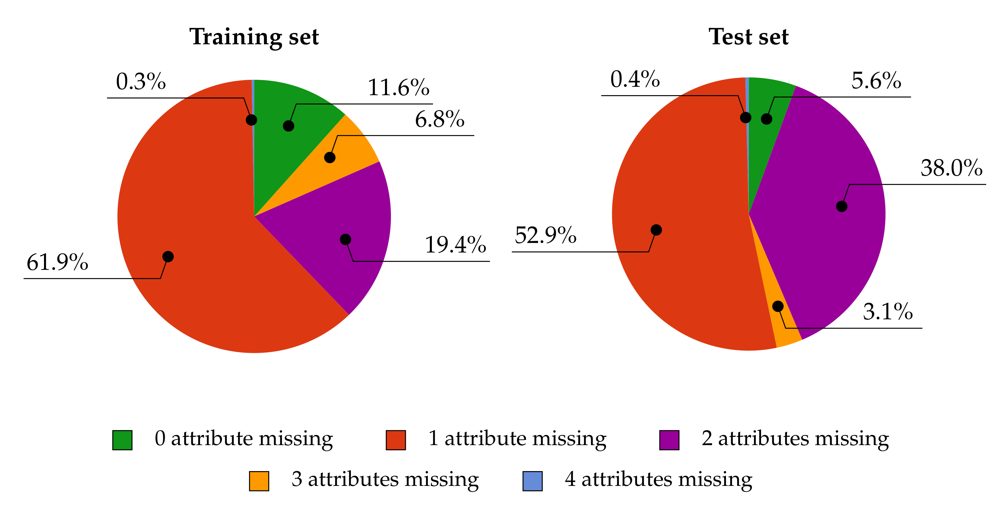
Since further analysis covers the number of missing values for individual attributes in the dataset, and its impact on the behavior of particular classification algorithms, the percentage share of POIs (along with the number of missing attributes in the training and test set) are presented in Figure 4.
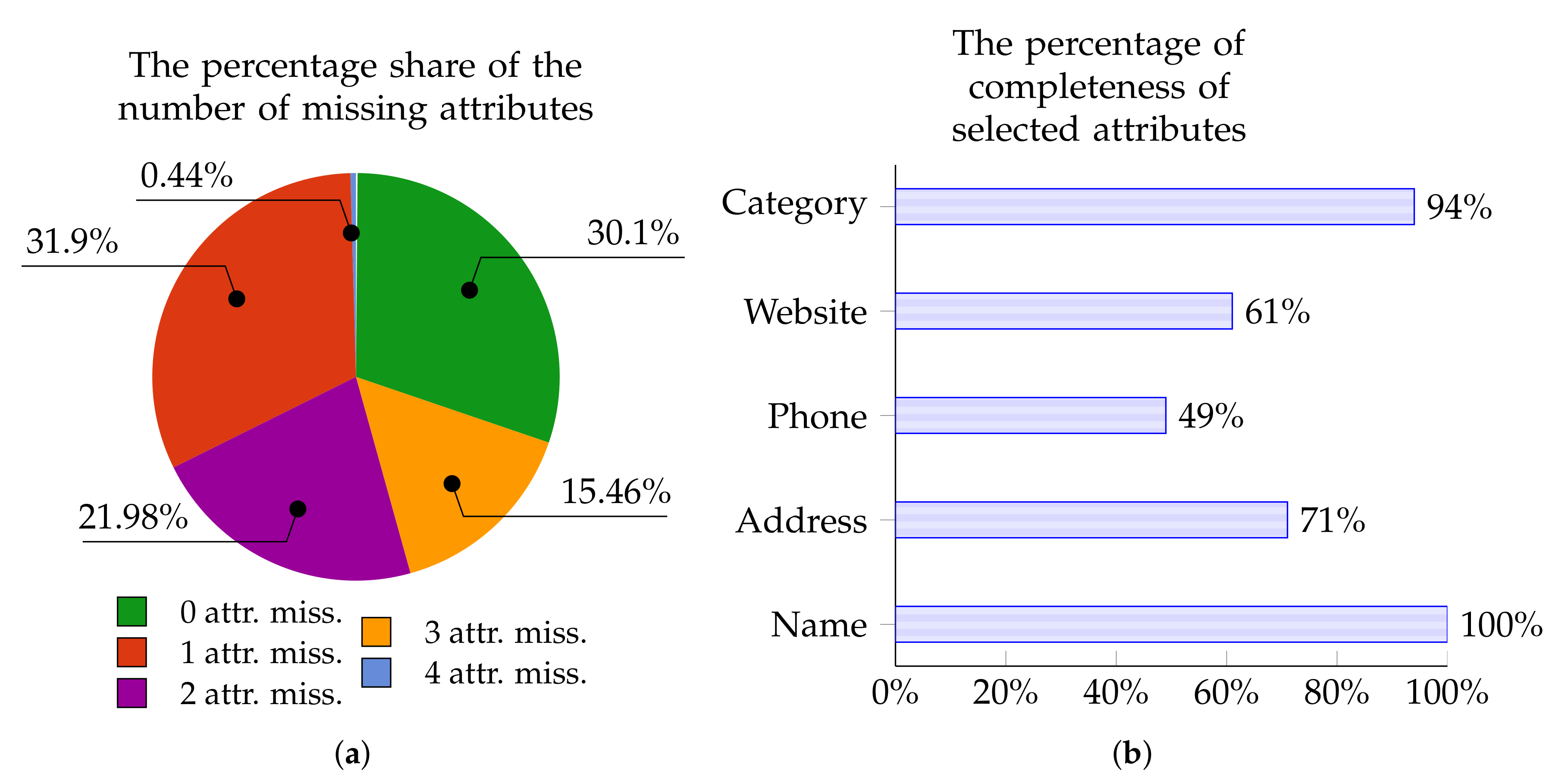
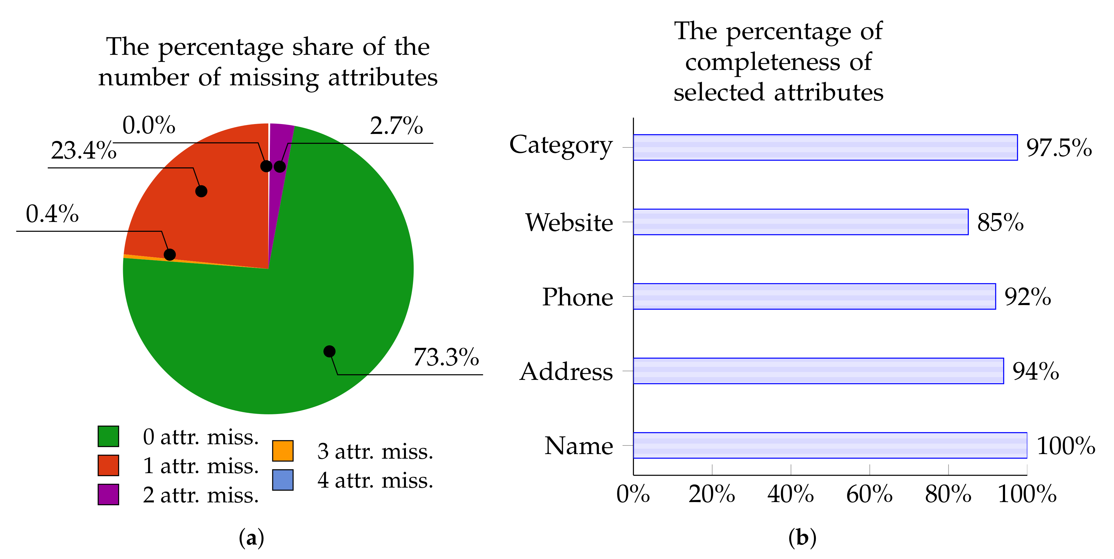
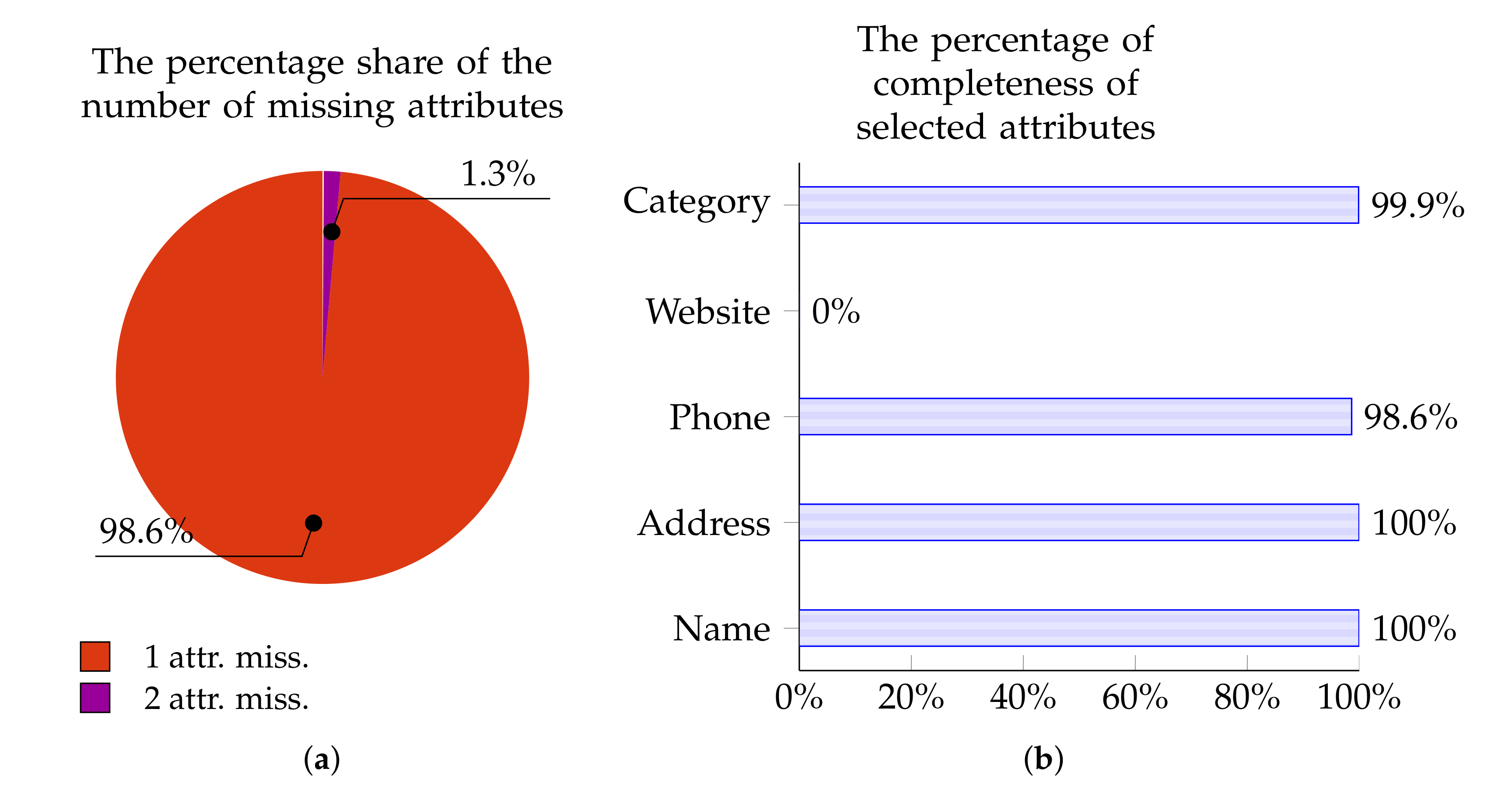
The charts below present the percentage of Points of Interest from individual data sources with zero, one, two, three, or four missing attributes. These charts—in Figure 5a, Figure 6a, Figure 7a, and Figure 8a—are for OpenStreetMap, Foursquare, Facebook Places, and Yelp, respectively.
Similarly, Figure 5b, Figure 6b, Figure 7b, and Figure 8b show the percentage of completeness for the five attributes of most interest: Name, Address, Phone Number, Website, and Category. Figure 5b describes the data from OpenStreetMap, Figure 6b characterizes the data from Foursquare, Figure 7b outlines the data derived from Facebook Places, and Figure 8b describes data for Yelp.
4. Crucial Elements of Points of Interest Matching Classifiers: Similarity Metrics, Handling Strategies for Missing Data and Classification Algorithms
The most important elements of Points of Interest matching classifiers are:
- the metrics for measuring the similarity of POIs;
- handling strategies for missing data; and
- algorithms for classifying Points of Interest as either matching or non-matching.
All these elements used in our research are discussed briefly in the following subsections.
4.1. Similarity Metrics
4.1.1. Distance Metrics
The most obvious approach to Points of Interest matching is to compare the (physical) distance between them. Knowing the geographical coordinates for the POIs being compared, and assuming that the points being compared are located a short distance apart, we can calculate the geographical distance in degrees () between them using the following formulas:
where
Now, having obtained the distance in degrees, we can calculate the distance in meters according to the following formula:
We intentionally avoided the use of a more accurate great circle distance and opted to use a simpler formula that ignores the curvature of the Earth. The reason is the fact that we are calculating the distance for relatively closely located objects (closer than 300 m). In that case, the curvature of the Earth can easily be omitted for our purposes. For example, sample distance values for two points located about 225 m from each other are 225.42 m when we use a great circle distance and 225.67 m with our formula. Simultaneously, the distance of 1 m represents a 0.003 difference in the value of our matching metric. Thus, since the difference is negligible, we decided to use this simpler, faster, and more efficient (i.e., less computationally complex) formula.
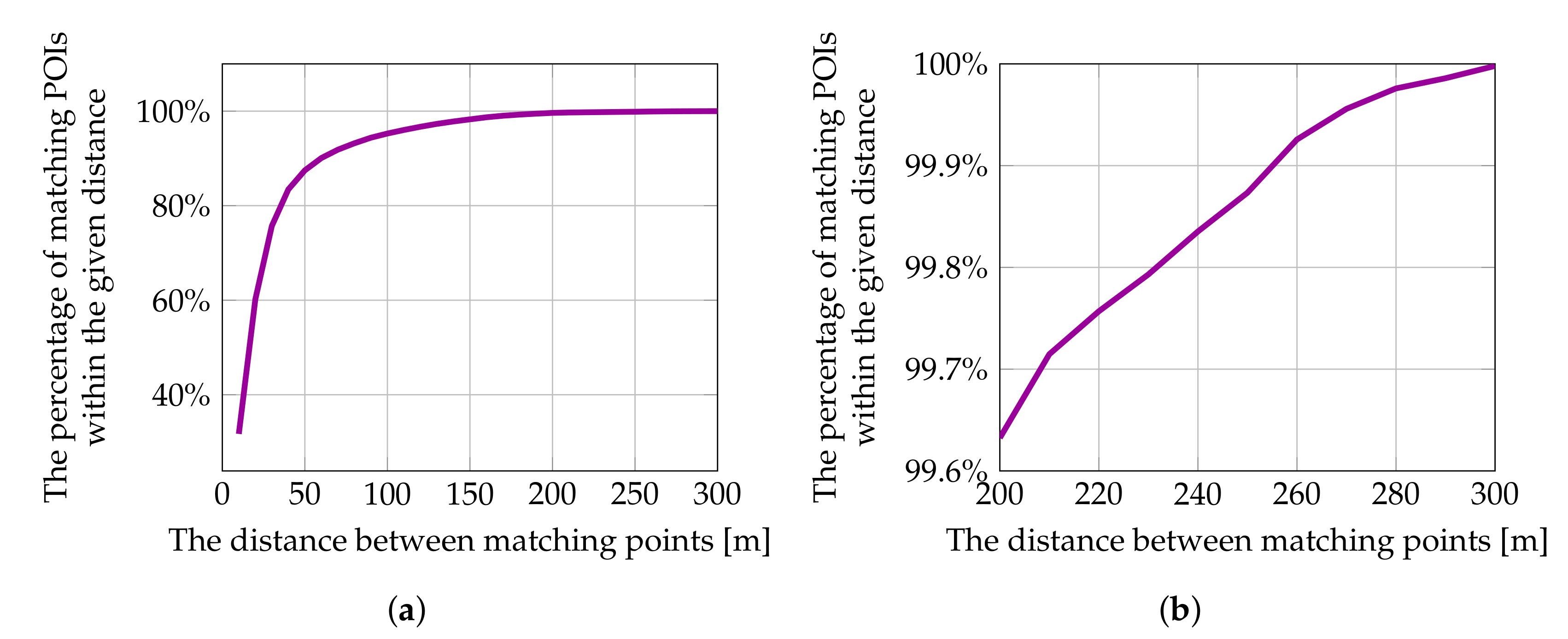
The range of 300 m in which we seek possible “matches” is an arbitrary choice, but one for which there is strong justification in the analysis we performed. Figure 9a presents the percentage of matching Points of Interest located within the range of 0–300 m. As can be seen, almost 100% of matching POIs are located no further than 300 m from each other. It would seem that the border distance could be set even closer (to 200 m), but since there are also some matching Points of Interest located within the range between 200 and 300 m (detailed in Figure 9b), in further analysis, we took the range of 300 m as the border distance in the search for matching Points of Interest. Thus, for further calculations and analyses, we took a normalized distance measure calculated according to the equation:
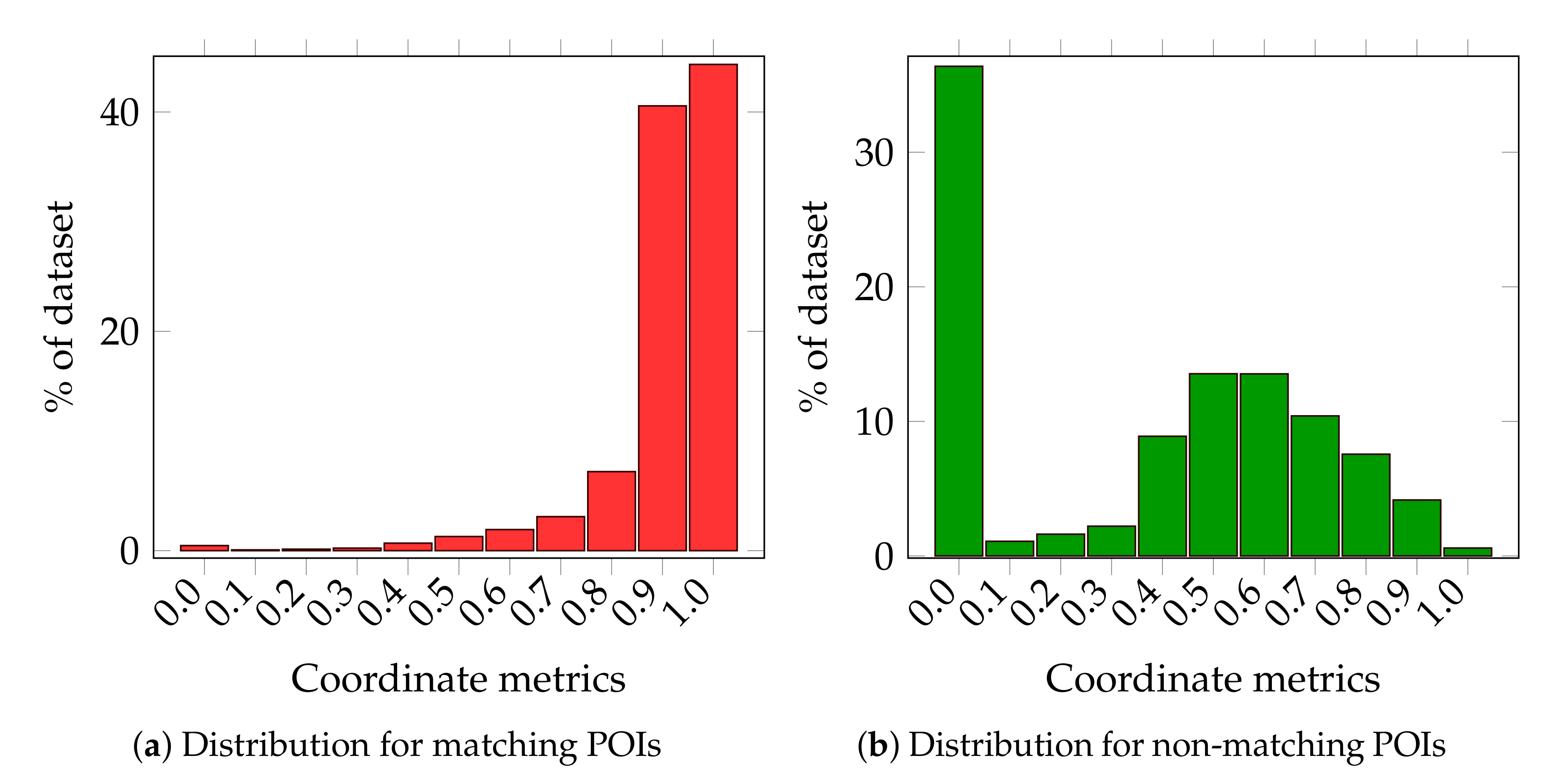
The distribution of in the training set for matched and mismatched Points of Interest are shown in Figure 10.
As we can see, this metric indicates the matching and non-matching Points of Interest very well. In the analyzed set, over 80% of matching objects display the value of this metric ranging from 0.9 to 1. At the same time, in a subset of mismatched points, over 35% of objects have the value of this metric equal to 0.
4.1.2. String Distance Metrics
The second approach to combining Points of Interest is to match their descriptive attributes (such as the name, address, phone number, etc.). To make this possible, it is necessary to determine the similarity between strings for specific attributes. There are many algorithms for string comparison. In our research, we used Levenshtein [2] and Jaro–Winkler [17] distances, as well as algorithms provided by the FuzzyWuzzy library [18], i.e., Ratio, Partial Ratio (PR), Token Sort Ratio (TSoR), and Token Set Ratio (TSeR). In addition, as in [5], we used a combination of the average value of Partial Ratio algorithm with Token Sort Ratio (ATSoR) and Partial Ratio with Token Set Ratio (ATSeR).
The Levenshtein distance is defined as the minimal number of operations that must be performed to transform one string into another [2]. The set of permissible operations includes:
- inserting a new character into the string;
- removing a character from the string; and
- replacing a character inside the string with another character.
To facilitate the analysis of string similarity as measured by the Levenshtein metric, the value of the metric determined for two non-empty strings should be normalized in the range from 0 to 1 and applied to the equation:
The Jaro–Winkler metric [17] determines the distance between two strings according to the equation:
where m is the number of matching characters, and t is half of the number of so-called transpositions (matching characters but occurring at different positions in the inscriptions being compared).
In other words, the Jaro–Winkler distance is the average of:
- the number of matching characters in both strings in relation to the length of the first string;
- the number of matching characters in both strings in relation to the length of the second string; and
- the number of matching characters that do not require transposition.
The algorithms implemented in the FuzzyWuzzy library provided by the Seatgeek group (https://chairnerd.seatgeek.com/fuzzywuzzy-fuzzy-string-matching-in-python/) are based on the Levenshtein metric, differing in their variants in the way they select string elements for comparison. All values representing the similarity of the strings are returned in the range [0,100], thus their normalization is achieved by dividing by 100. The FuzzyWuzzy strings similarity measures are as follows:
- The Ratio () is a normalized similarity between the strings calculated as the Levenshtein distance divided by the length of the longer string.
- The Partial Ratio () is an improved version of the previous one. It is the ratio of the shorter string and the most similar substring (in terms of the Levenshtein distance) of the longer string.
- The Token Sort Partial Ratio () sorts the tokens in the string and then measures the Partial Ratio on the string with the sorted tokens.
- The Token Set Partial Ratio () creates three sets of tokens:
- -
- , the common, sorted tokens from two strings;
- -
- , the common, sorted tokens from two strings along with sorted remaining tokens from the first string; and
- -
- , the common, sorted tokens from two inscriptions along with sorted remaining tokens from the second string.
Then, strings as a combination of tokens in the set are created and the maximum Partial Ratio is computed according to the equation: - The Average Ratio () is the metric we proposed, calculated as the average value of the Partial Ratio (PR) and the Token Set Ratio (TSeR):
Table 1 compares the values of these metrics obtained for the sample strings. The following notations for individual metrics are adopted in the table:
- is the Levenshtein measure.
- is the Jaro–Winkler measure.
- is the Ratio measure.
- is the Partial-Ratio measure.
- is the Partial Token Sort Ratio measure.
- is the Partial Token Set Ratio measure.
- is the Average Ratio measure.
4.1.3. Category Distance Metrics
Choosing the right metrics when comparing categories is more complex than in the case of (simple) attributes such as the Name. This is because their comparison should be based on semantic rather than textual similarity. This is evident when we take, for example, Hostel and Bed and Breakfast categories. Semantically, they are very close while their string similarity is close to zero.
In this context, we analyzed several semantic comparison techniques including the Sorensen algorithm proposed in [5] and semantic similarity metric based on the Wordnet dictionary (https://wordnet.princeton.edu/) with the implementation provided by NLTK library (https://www.nltk.org/) [19]. For further experiments and analysis, we selected Wu–Palmer, Lin, and Path metrics. Additionally, we conducted some experiments using two- and three-element combinations of these metrics. Since the category is a multi-valued attribute (e.g., “Food”, “Restaurant”, and “Polish”), we decided to select and compare the last two values for each category. Next, we created a Cartesian product from these two last categories for the POIs being compared, and used the value of the most similar pair. Formally,
where is the set of categories for the point and is the similarity of the categories and .
4.2. Strategies for Dealing with Missing Data
In the experiments, we assessed four strategies for handling the problem of missing and/or incomplete data:
- is a strategy in which only objects with all attributes are taken for testing and analysis. This is not an approach that can be used in practice, but it was carried out merely to obtain a reference result.
- is a strategy where, in the training set, we only include objects that have all the attributes, and, in the test set, we fill in the missing values with a marker value: −1.
- is a strategy where, in both sets, we fill in the missing values with the marker value: −1.
- is a strategy in which missing values are supplemented with the median value of the attributes in the given set.
4.3. The Classifiers for Points of Interest Matching
The selected classifiers for Points of Interest matching used in our research are briefly enumerated below:
- The k-Nearest Neighbor algorithm [20] is one of the most popular algorithms for pattern determination and classification. The classifier based on this algorithm allows one to assign an object to a given class using a similarity measure. In the case of the Points of Interest matching problem, based on the given values of the metrics, the algorithm looks for similar examples encountered during the learning process. After that, it endeavors to qualify them into one of two groups—matching or mismatching objects. In our analysis, we used the implementation provided by the Scikit Learn Framework [21]. We used the default parameters configuration (https://scikit-learn.org/stable/modules/generated/sklearn.neighbors.KNeighborsClassifier.html), changing only the parameter value, which indicates the number of neighbors sought; we changed it from 5 to 100, due to the large dataset.
- The Decision Tree classification method [22] is a supervised method, and, on the basis of the datasets provided, it separates objects into two groups. The separation process is based on a chain of conditionals, which form a graphical tree. One of the disadvantages of this algorithm is that the decision tree is very susceptible to the prepared learning model. This is due to overfitting, and the lack of a mechanism to prevent the dominance of one resultant class. Therefore, we had to ensure that the training set was well balanced. In our analysis, we again used the implementation provided by the Scikit Learn Framework [21]. We used the default parameters configuration ( https://scikit-learn.org/stable/modules/generated/sklearn.tree.DecisionTreeClassifier.html). In our model, we had six input features (metrics values for two Points of Interest being compared), and two output classes (objects matched or not).
- The Random Forest classifier [23] is based on the same assumptions as those of the decision trees. However, unlike a single decision tree, it does not follow the greedy strategy when creating the conditionals. In addition, the sets provided for training individual trees are different. As a consequence, the algorithm is more resistant to overfitting phenomena and is well-suited to missing data. In our analysis, we once again used the implementation provided by the Scikit Learn Framework [21]. We used the default parameters configuration ( https://scikit-learn.org/stable/modules/generated/sklearn.ensemble.RandomForestClassifier.html), changing only the number of trees in the forest ( parameter) to 100.
- Isolation Forest is the method of matching objects studied in [5,6]. It is based on the outlier detection approach. This classifier, unlike those previously presented, is a weakly supervised machine learning method where, in the training process, only the positive examples are required. Next, during the classification process, the classifier decides whether the given set of attributes is similar to those that it has learned in the learning process or not. The algorithm is very sensitive to the data used and requires appropriate techniques in the case of missing attributes. In our analysis, we again used the implementation supplied by the Scikit Learn Framework [21]. We used the default parameters configuration (https://scikit-learn.org/stable/modules/generated/sklearn.ensemble.IsolationForest.html), setting the number of samples used for training (i.e., the parameter) to 1000.
- Neural Network: We prepared two classifiers based on a Neural Networks [24]. The simpler one, termed a Perceptron, directly receives the values of the metrics, and the two output neurons are the resultant classes—the decision about any similarity or lack thereof. A more complicated one, based on deep networks, is the Feed Forward model, which in addition to the input and output layers, has six additional, arbitrarily set layers, with 128, 64, 32, 16, 16, and 16 neurons, respectively. In our analysis, we used the implementation provided by the Tensorflow [25] and Keras [26] frameworks. We trained each of the networks for 50 eras, with the batch size set to 5.
As the input to all classifiers, we provided the vector of six metrics values, normalized into the range of [0,1] and representing, in turn, geographical proximity, and then the name, addresses, phone numbers, websites, and categories similarity.
5. Experiments
To compare the selected classifiers with different metrics and strategies for dealing with missing data, we performed a series of experiments on the experimental dataset. The question is how to determine which classifier is better than the others. One of the most popular classification quality indicators is the Receiver Operating Characteristic curve (ROC) [27] along with the Area Under the ROC field (AUC). An AUC value of 1 means it is an ideal classifier. An AUC equal to 0 is characteristic of an inverse classifier. An AUC value of 0.5 indicates that we are dealing with a random classifier. The values of ROC and AUC are presented in later analyses.
5.1. The Analysis of Different Similarity Metrics
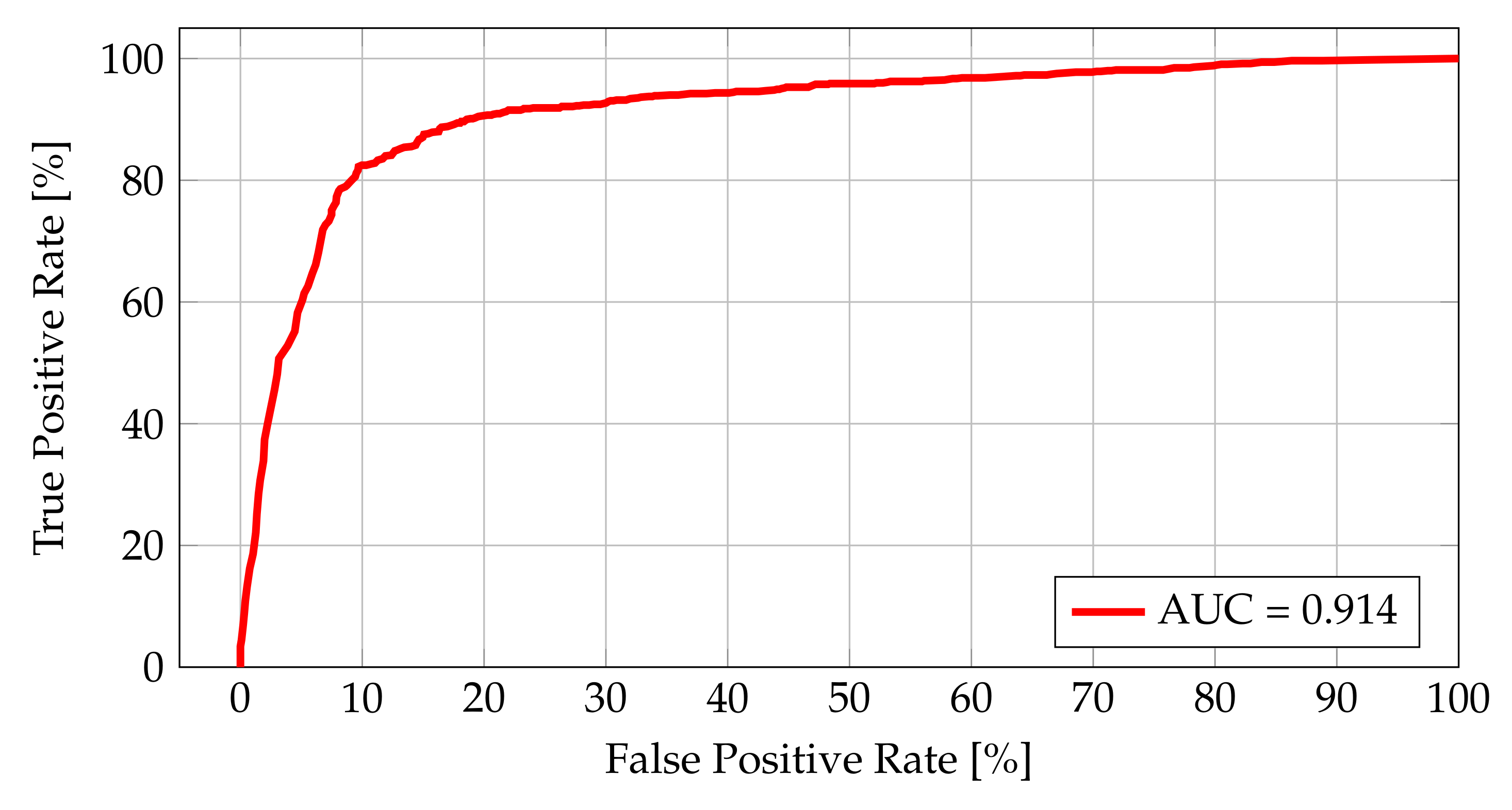
The ROC curve along with the AUC value for the geographical closeness estimation metric are shown in Figure 11. The obtained value of AUC (0.914) shows that the metric proposed is accurate and can be used for the POI matching classification. The assumed range of 300 m is adequate to make a fair classification for two objects being compared and reduces the impact of any GPS inaccuracy [28].
5.1.1. The Analysis of String Similarity Metrics
The results obtained for different string similarity metrics calculated for different attributes are presented in the following subsections. In the interests of space and brevity, the reader may refer to Appendix A to find the detailed characteristics of the ROC curves and the AUC values. Below, we provide a summary of the results.
The Analysis for the Attribute Name
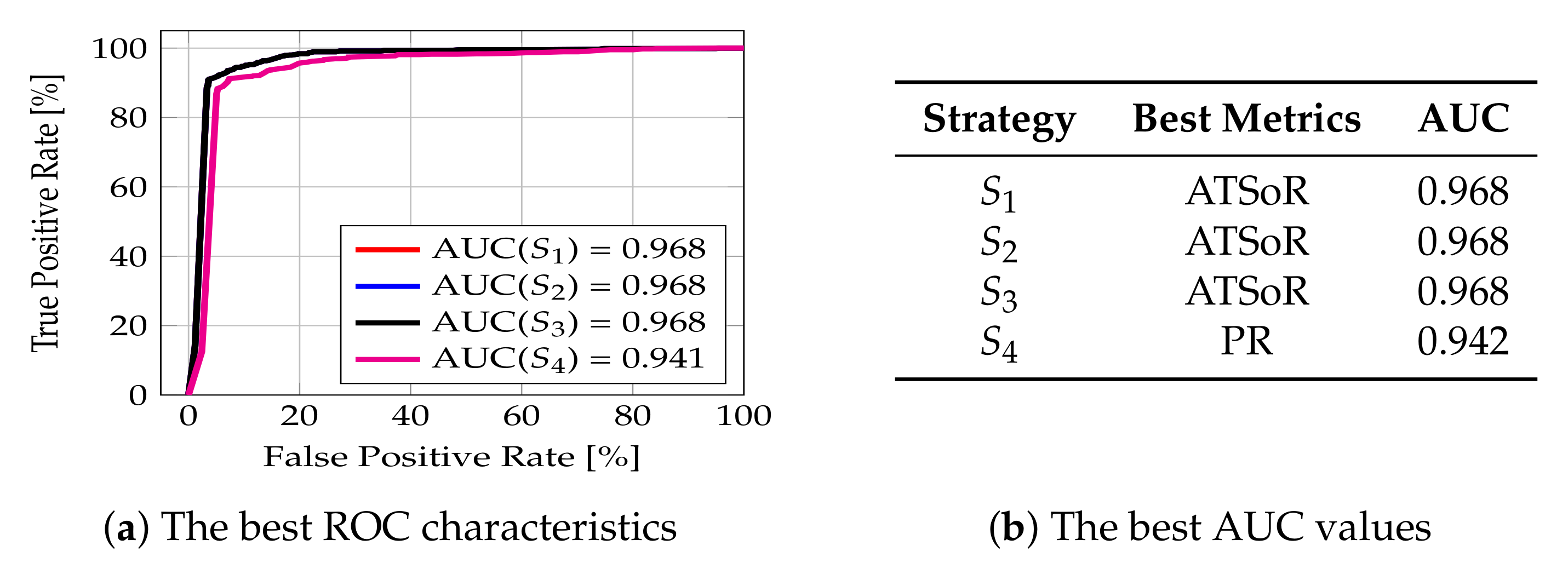
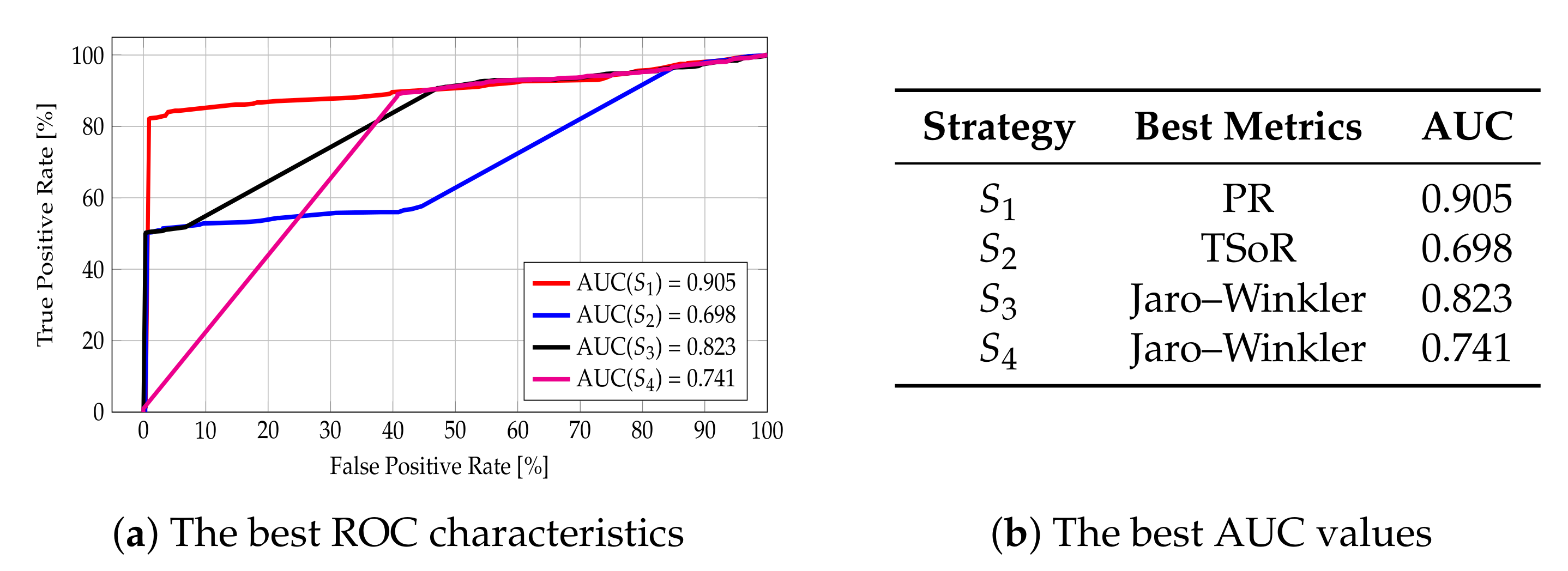
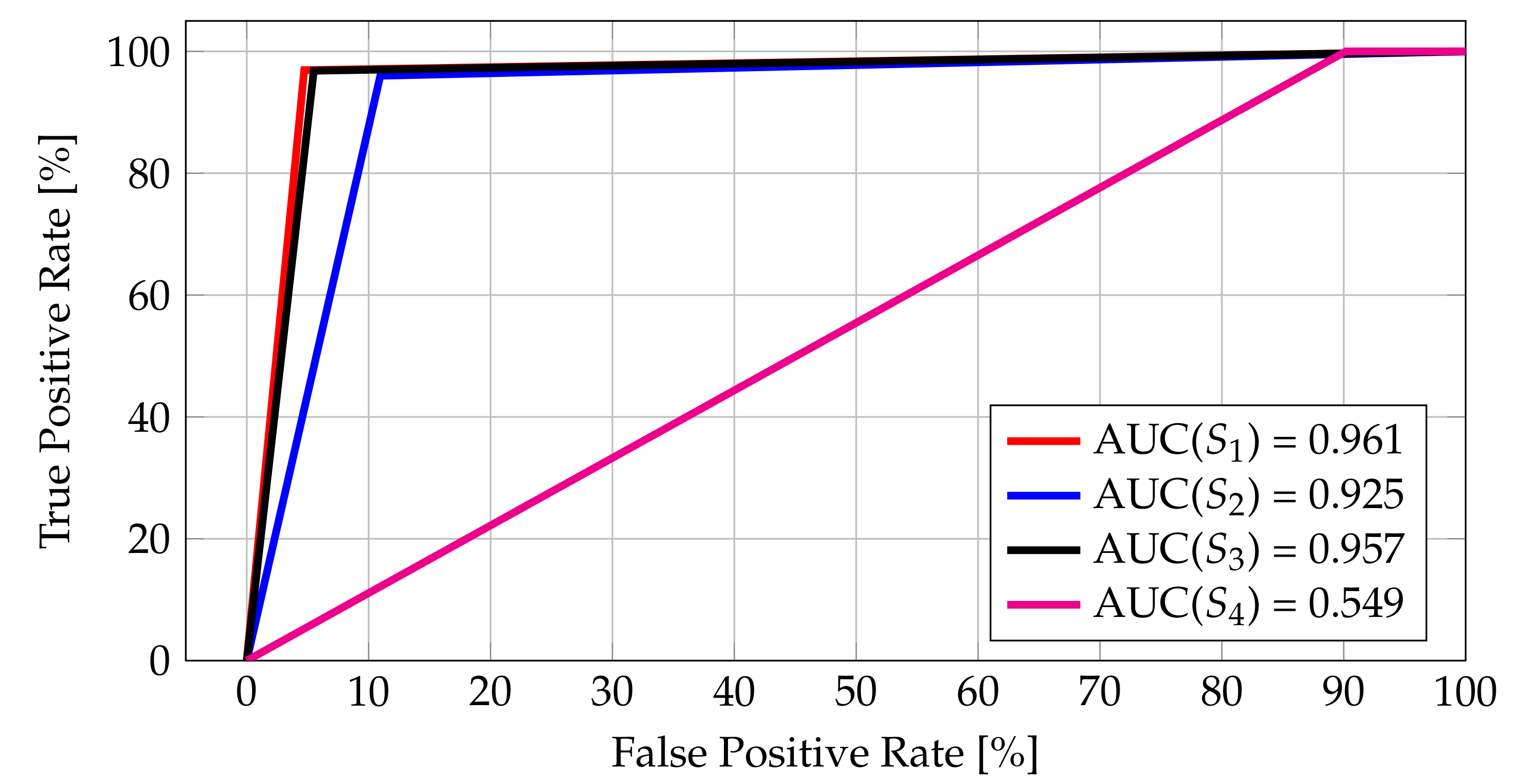
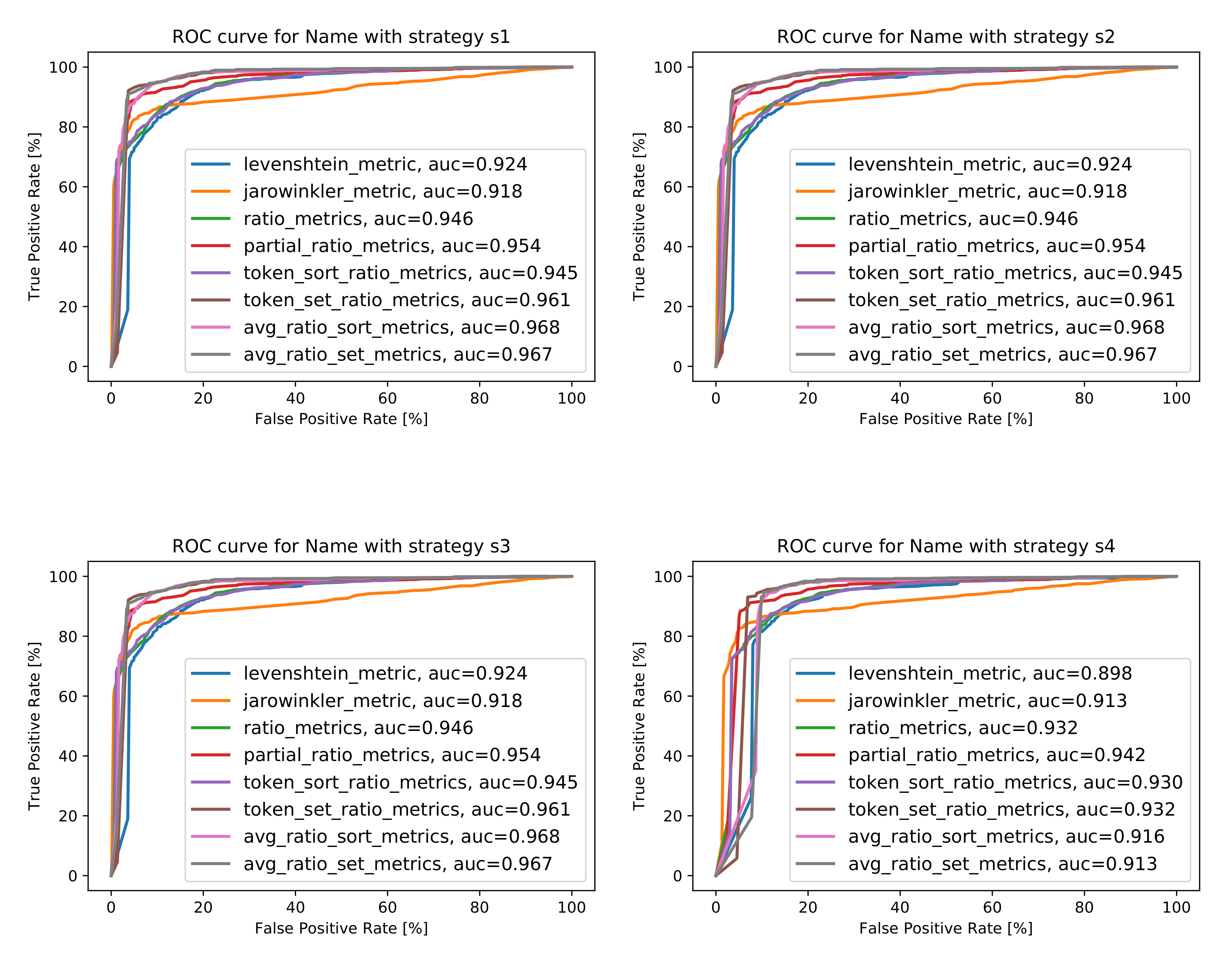
When it comes to the Name attribute, the best area under the curve value for strategy was obtained with the Average Token Sort Ratio metric (ATSoR) and is equal to 0.968. The same can be observed for strategies and , whereas, for strategy , the best AUC value, equal to 0.942, was obtained with the Partial Ratio metric. The reason for that is that the Name attribute often appears in reverse order, for example “Hotel X” and “X Hotel”; thus, it is to be expected that the best value was obtained with the use of the sorting metric. The same applies when it comes to Partial Ratio metrics, comparing the similarity of words based on the length of individual tokens. The values obtained are high, which indicates that the selected metrics are able to classify the strings correctly. For clarity and ease, the best AUC values obtained, along with the information concerning the metrics for which these values were obtained, are collected in Figure 12b, while the ROC curves for best cases are presented in Figure 12a. More detailed characteristics can be found in Figure A1 in Appendix A.
The Analysis for the Attribute Address
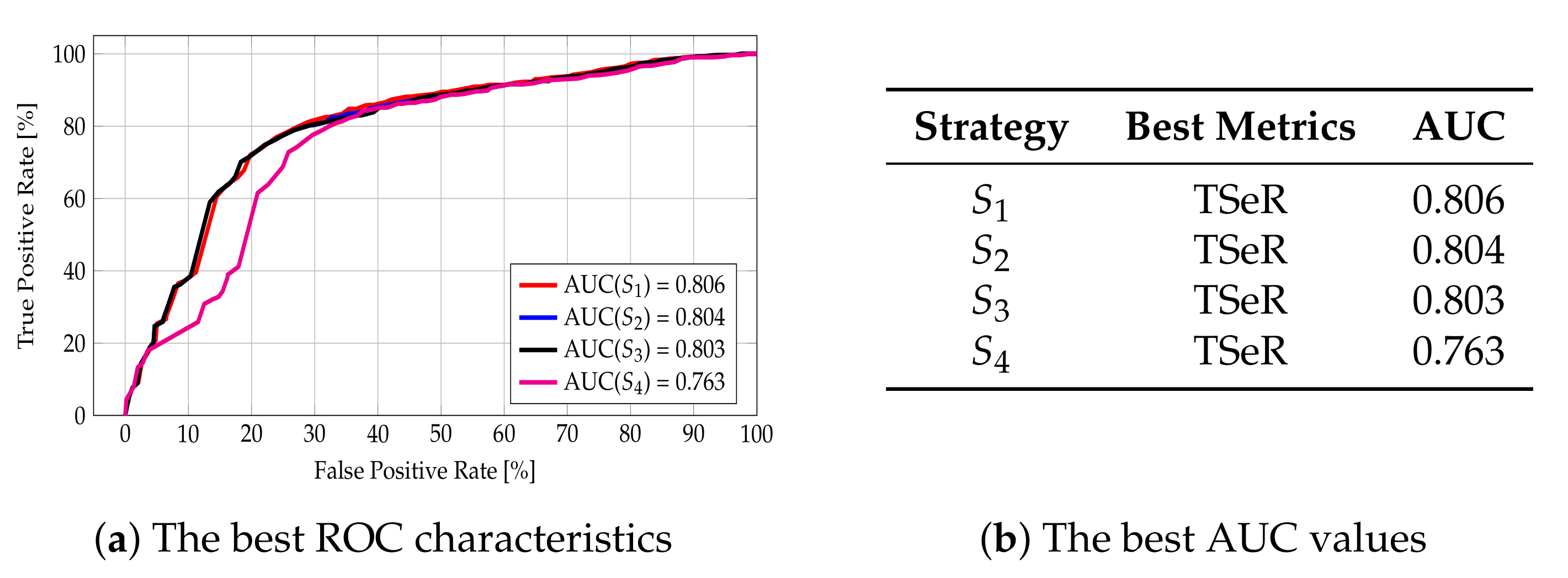
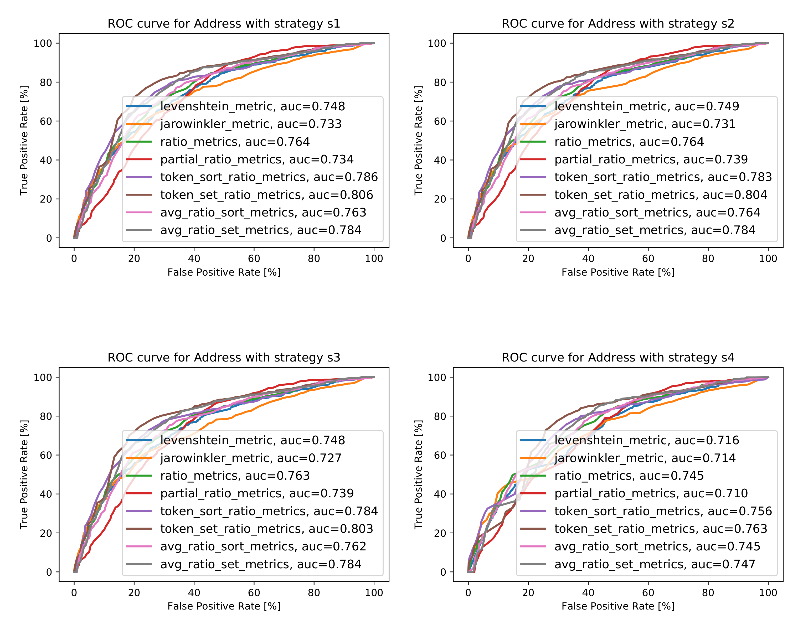
In the case of the Address attribute, the best area under the curve value for strategy was obtained with the Token Set Ratio (TSeR) and equals 0.806. The same metric also yielded the best AUC values for strategies , , and ; it was equal to 0.804 for strategy , 0.803 for strategy , and 0.763 for strategy . These results stem from the fact that the address is given in a standardized format: Street, House Number, ZIP code, City, Country. Therefore, the tokens are already sorted, and the comparison of strings comes down to the comparison of particular tokens. The values obtained are fairly high, but this metric does not separate objects as well as in the case of the name attribute because neighboring places located on the same street may differ only in House Number token, although they are completely different POIs. The best AUC values gained, along with the information about the metrics for which these values were obtained, are collected in Figure 13b, and the ROC curves for best cases are depicted in Figure 13a. Further details are given in Figure A2 in Appendix A.
The Analysis for the Attribute Phone Number
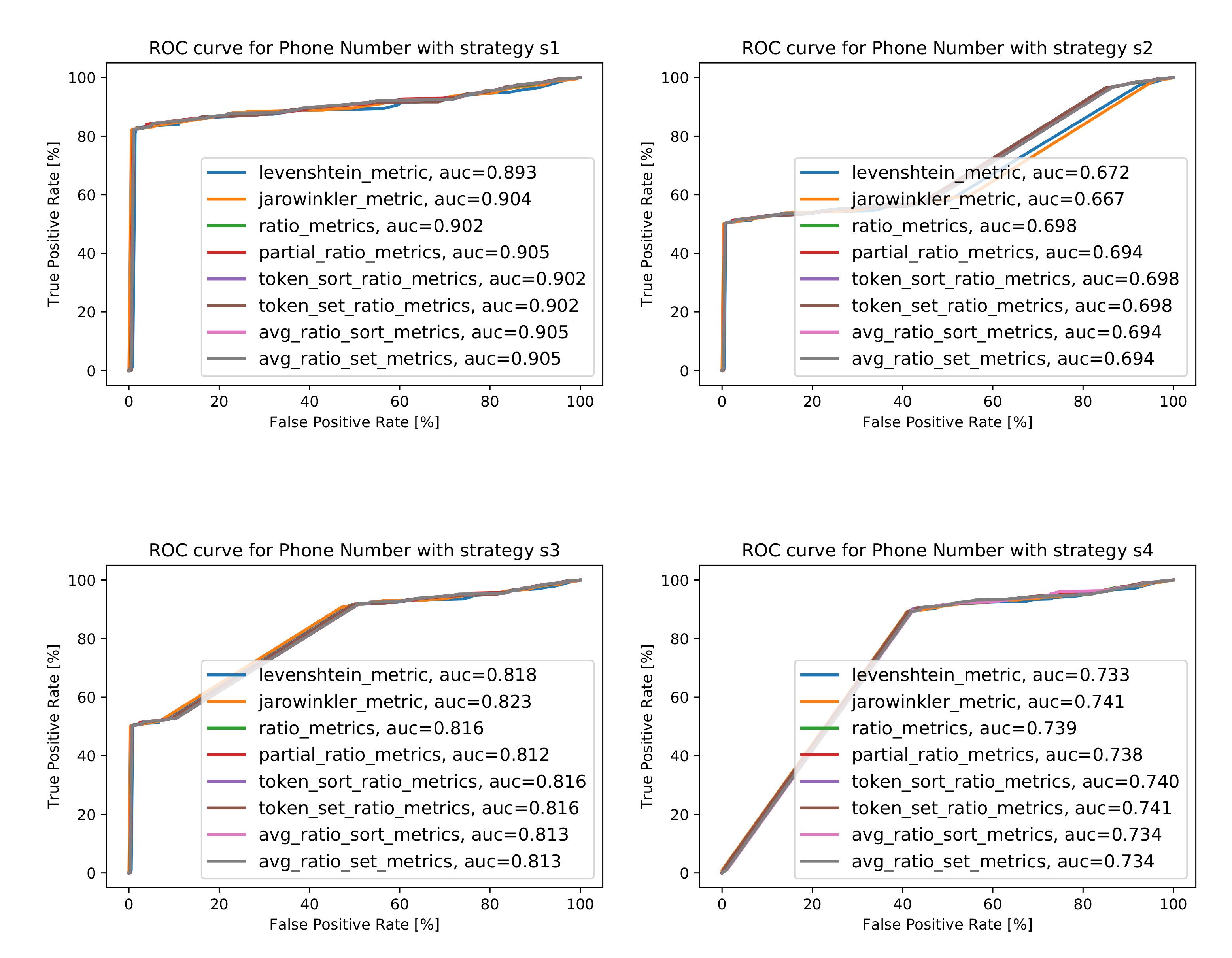
The comparison and matching of the Phone Number attribute is a greater problem than for Name or Address—as can be seen in the varying results of the metrics and the AUC values. In the case of strategy (an ideal dataset where all pairs have a phone number), it can be seen that the simple metric does well—reaching an AUC value above 0.9. The best results (apart from the ideal dataset) were obtained for the strategy along with the Jaro–Winkler metric—which is based on the number of modifications of one string as compared to another. This makes sense because a phone number is already a standardized string of characters without taking the prefixes into account.
The best AUC values obtained, along with the information concerning the metrics for which this value was obtained, are collected in Figure 14b, and the ROC curves for best cases are presented in Figure 14a. Detailed characteristics are shown in Figure A3 in Appendix A.
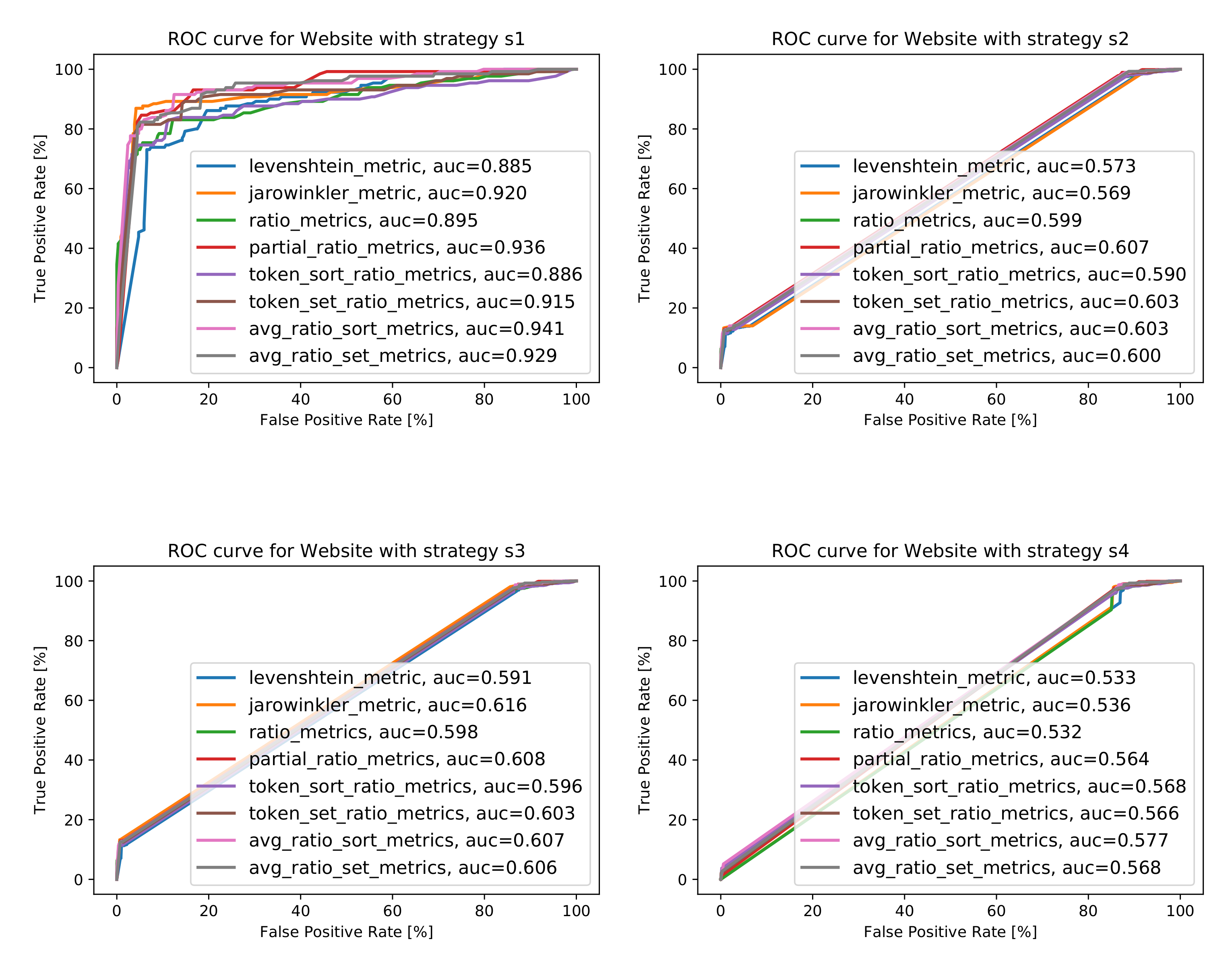
The Analysis for the Attribute WWW
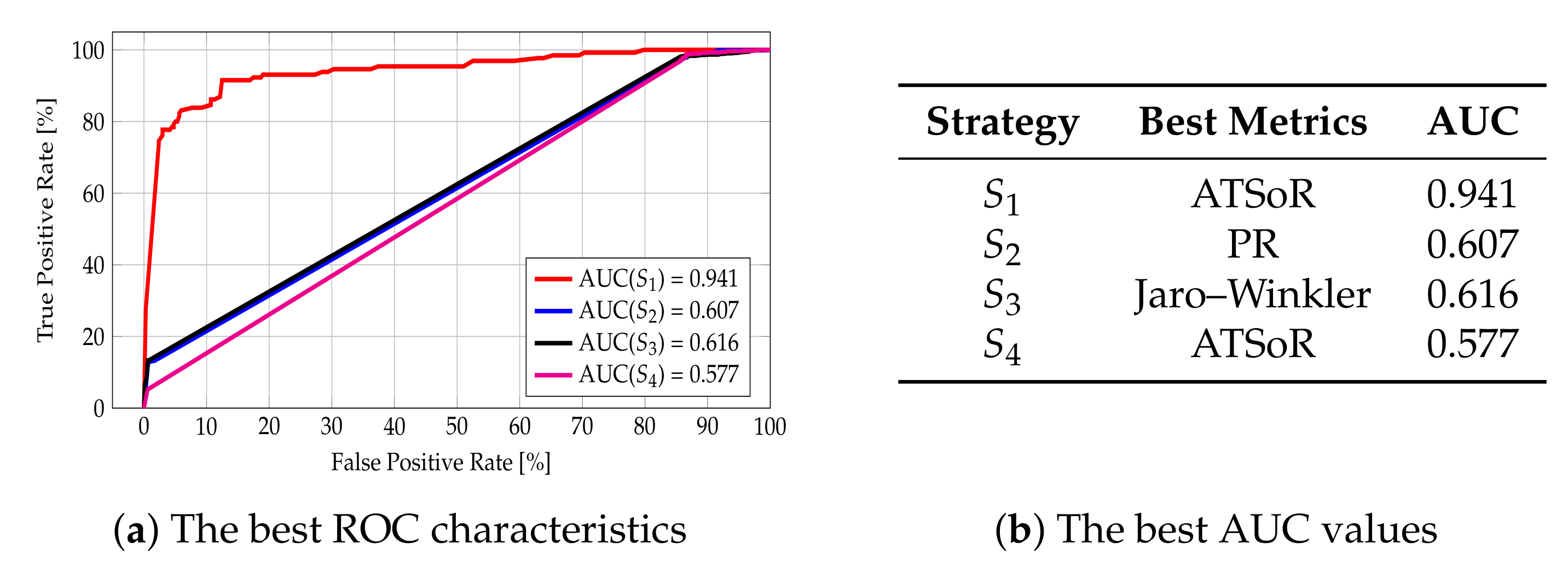
The worst particular metrics values (compared to those attributes discussed thus far) were obtained. While, for the ideal dataset (strategy ), the results are high (AUC = 0.941 for ATSoR metrics), for the other strategies, the values are close to being random classifiers. This stems from the fact that only about 30% of objects in the experimental set have a value for this attribute. Nevertheless, this attribute is still worth taking into account when creating the Points of Interest matching classifier because, if the object already has the value of this attribute, the relevance of matching is reasonably high. The best AUC values obtained, along with the information about the metrics for which these values were acquired, are collected in Figure 15b, while the ROC curves for best cases are presented in Figure 15a. Greater detail can be found in Figure A4 in Appendix A.
The Analysis for the Combination of Attributes
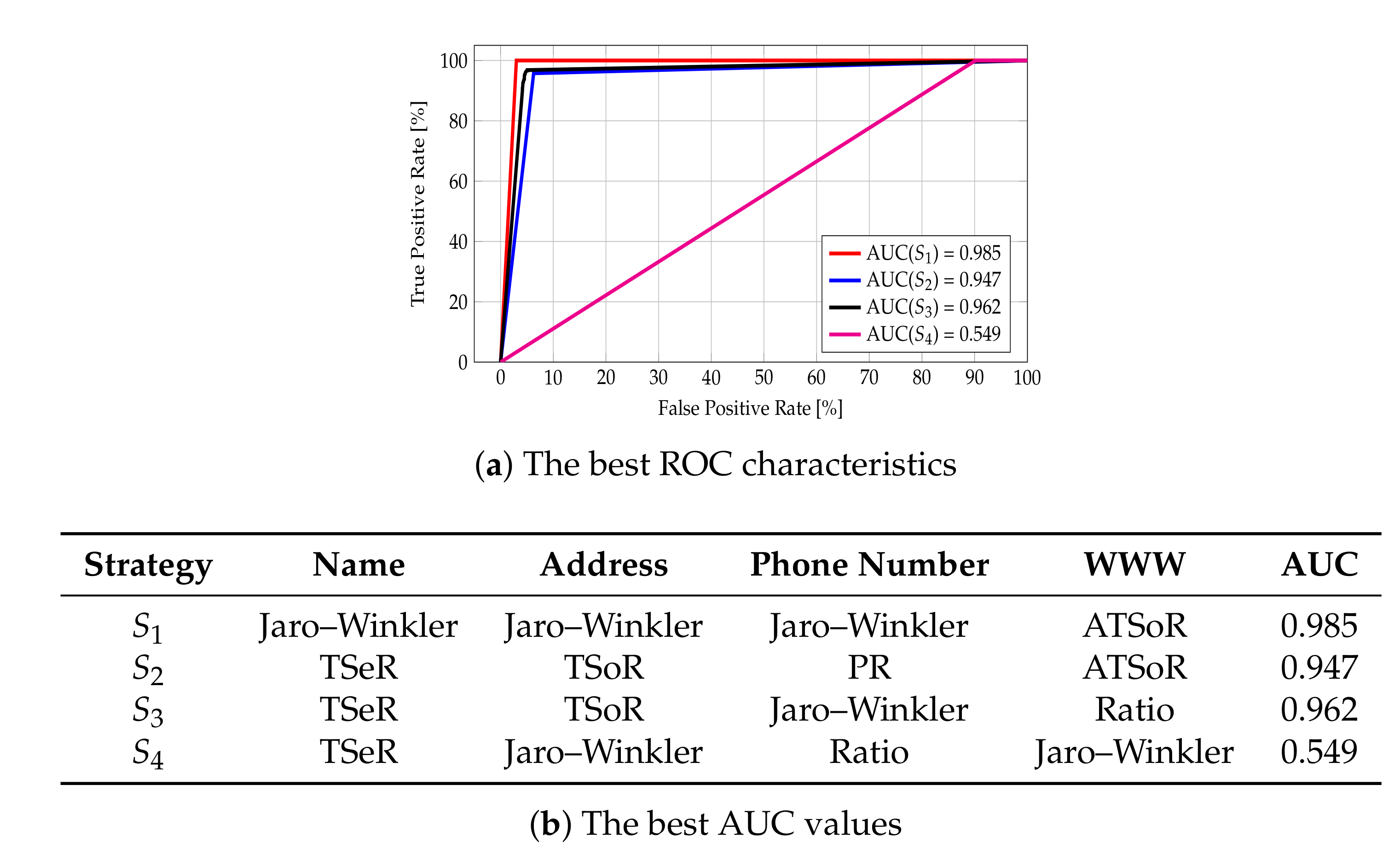
Finally, we checked whether the results for individual attributes are reflected in the classifier using the combination of attributes. The best AUC values obtained, along with the information about the metrics for which the values have been obtained, are collected in Figure 16b, and the ROC curves for the best cases are presented in Figure 16a. Analyzing the results, it can be seen that the best results for individual strategies and attributes do not translate directly into a “mixed” model.
5.1.2. The Analysis for Category Distance Metrics
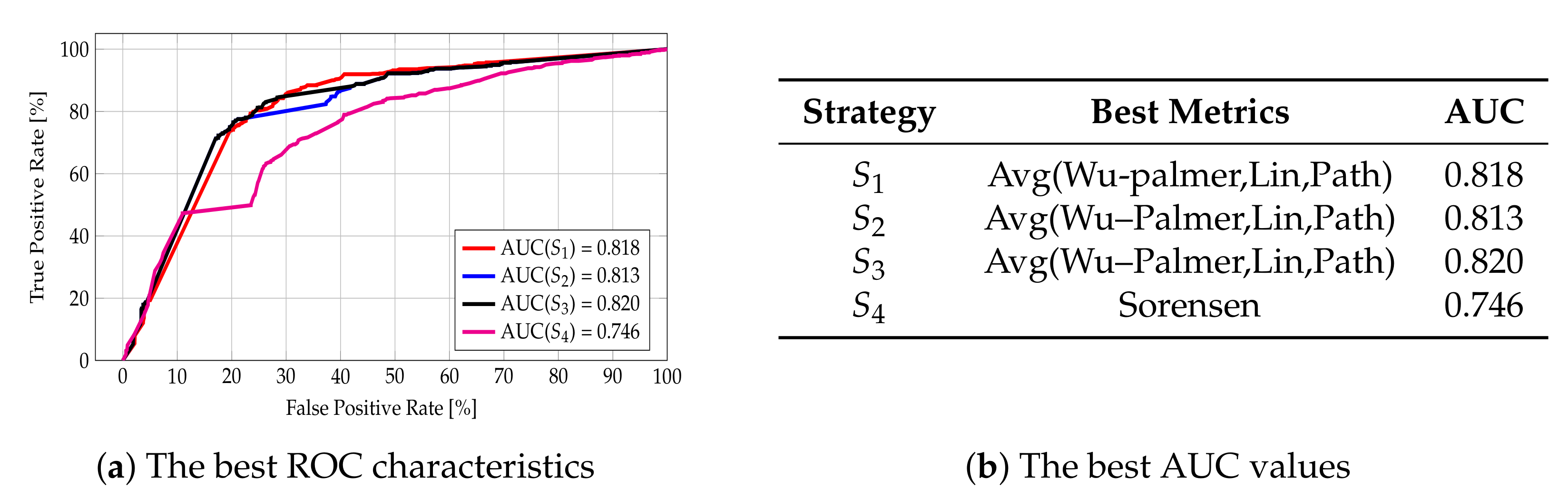
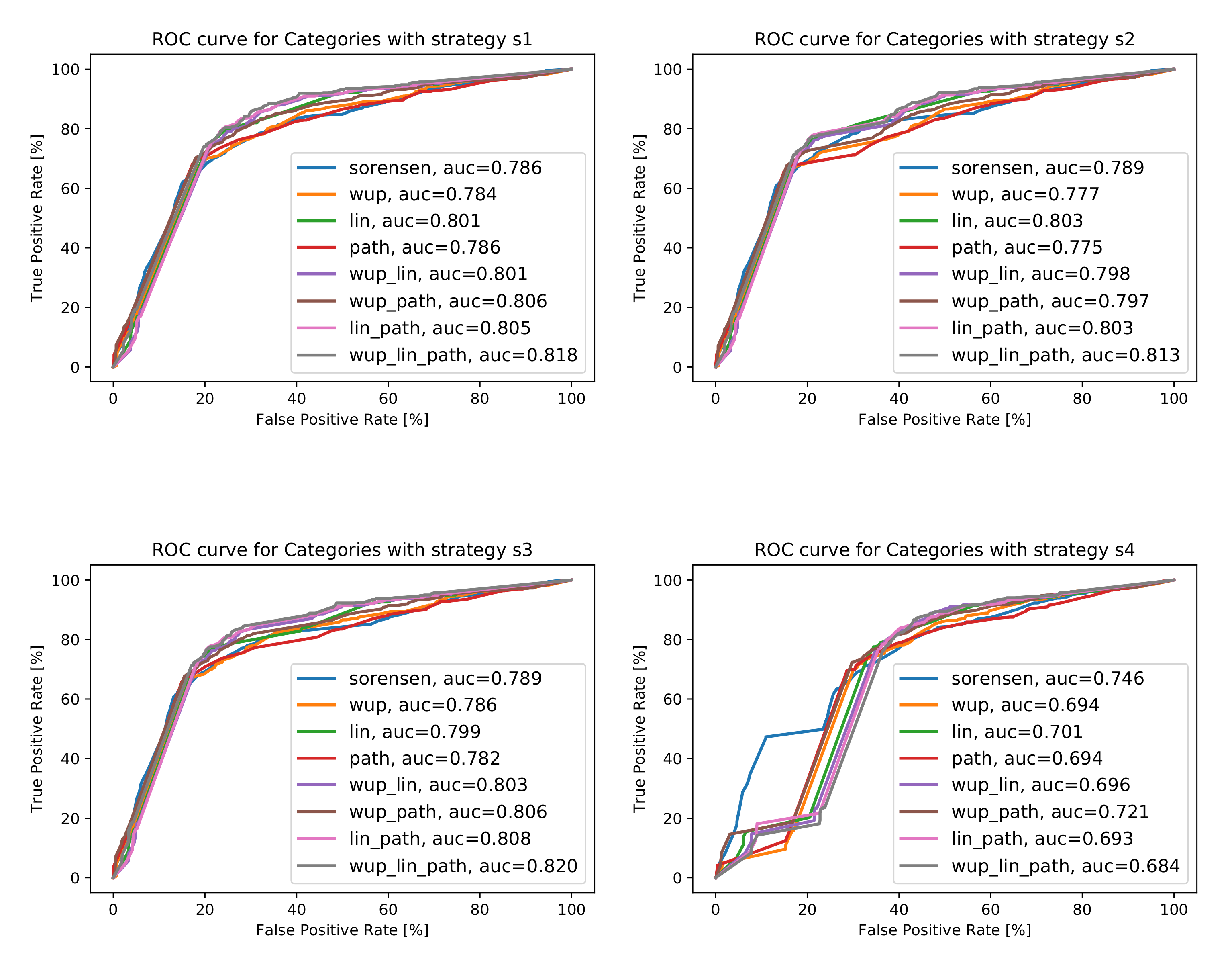
Category metrics were tested for various strategies for dealing with missing data, and a summary of the results is presented in Figure 17. For strategies , , and , the best AUC values were obtained with the average of Wu–Palmer, Lin, and Path metrics; these were 0.818 for strategy , 0.813 for strategy , and 0.820 for strategy . For strategy , the best AUC value, equal to 0.746, was attained with the Sorensen metric.
The best AUC values gained, together with the information about the metrics for which these values were obtained, are collected in Figure 17b, and the ROC curves for best cases in Figure 17a. More detailed information is in Figure A5 in Appendix A.
5.1.3. The Analysis for Combined Metrics
The last analysis of the metrics focused on checking the quality of the classifier based on the combination of three kinds of metrics, i.e., metrics for measuring the geographical closeness, string similarity, and category similarity. In this step, we took the most effective metrics from all three categories and built a classifier using all three at once. The basic conclusions we can draw based on the results obtained (see Figure 18) is that, in the case of the strategy, we are close to having a random classifier, whereas strategy gives results very close to the results for the “ideal” set (strategy ).
5.2. Comparison of Different Points of Interest Matching Classifiers
With a set of metrics for each strategy for handling incomplete data in hand, we proceeded to the next stage of our research, which was to compare various approaches of machine learning classifiers to Points of Interest matching. We selected six different machine learning classifiers and tested them on prepared datasets, applying selected metrics and strategies for dealing with incomplete data. The performance results for each classifier are collected in Table 2.
The analysis of the results showed that, for the ideal dataset (where all attributes are available), i.e., for strategy , the deep feed-forward neural net works best. The difference and advantage over the other classifiers is not large, however, since the lowest achieved efficiency is as high as 93.2%. The approach of and , which supplement the missing values with the −1 marker, shows that the results are not much worse than in the case of strategy —especially with regards to “tree-based” classification algorithms.
Neural nets achieve worse results with and than in the case of strategy because they are sensitive to the quality of the data provided. The other interesting result, confirming the findings presented in [5], is that obtained by the isolation forest algorithm for strategy . Being the only one capable of dealing with data with missing values, in this case, it achieved a superior result when compared to strategies and .
In addition, in Table 3, we present the results for individual cities in the best combination achieved, i.e., random forest with strategy . It is worth noting that high results are achieved in most cities, but there is an anomalous result for Liverpool. This means that selecting the best classification algorithm and the best metrics also depends on the region of the world (e.g., how the address attribute is provided, how “dense” the area is, etc.). It also leaves space for continuing research, which will take into account the use of various metrics and classifiers depending on the specificity of the data.
6. The Algorithm for Automatic Points of Interest Matching
The final stage of our research involved the preparation of an algorithm proposal that could be used to match geospatial databases automatically. The algorithm devised consists of several steps, the first being the selection of candidates that may potentially be a matching Point of Interest for a particular POI currently under analysis. Based on the results presented in Section 4.1.1, with an accuracy of 99.9%, we can assume that a possible ”match” for a given point is located within 300 m. Thus, for candidates selected from the integrated database within a range of 300 m, we calculate the metrics and pass them on to a trained machine learning classifier. Then, we choose Points of Interest that have been classified as matching and sort them in descending order by the average value of the calculated similarity metrics. Finally, as the matching Point of Interest, we take the first one from the sorted list. If the list is empty, the Point of Interest is marked as “new” (devoid of matching duplicates), otherwise we merge data for matched POIs. Since the aim of the research reported was seeking matching Points of Interest, we did not focus on merging data for matched POIs and, at this stage, when we hit the merging step in the matching algorithm, we applied a few simple rules to produce an integrated Point of Interest. Thus, assuming that the is the POI we seek the matches for, and the is the matching POI found, the rules are as follows:
- If the attribute exists in , we use it as the value for merged POI.
- If the attribute is missing in and exists in , we use the value from for merged POI.
- The value for category attribute for merged POI is the sum of and categories.
The improvement of the merge technique (e.g., how to merge address when, for instance, in we have a street and in we have a house number) was not considered in this research and is one of the future work directions.
The algorithm presented in Algorithm 1 is accurate—it checks all the possibilities and searches for the best possible solution. This leads to high computational complexity and a long operation time because metrics and classification are calculated and performed for each pair of POIs, which can be especially problematic in densely built-up areas. For this reason, we deployed the greedy version of this algorithm, in which we take advantage of a database engine, namely the full-text search mechanism, to sort candidate ”matches” using the previously indexed Name. The pseudo-code of this modified version is presented in Algorithm 2.
For both versions of the POI matching algorithm, the worst-case complexity is: where N is the number of Points of Interest for which we wish to find matching points, is the ith Point of Interest from the list of POIs for which we wish to find matching points, and is the -th candidate POI found within 300 m from POI .
Both versions of the algorithm were confronted with a validation set consisting of 4000 manually annotated points. It gives an overview of the quality of the proposed approach, as well as shows the impact of the modifications proposed in the greedy version. The Accuracy achieved (in the sense of the previously defined metric), the percentage of matches not found (even though they existed), and the percentage of incorrectly made matches by both versions of the algorithm are collected in Table 4.
| Algorithm 1: Automatic Points of Interest matching—precise version. |
 |
| Algorithm 2: Automatic Points of Interest matching—greedy version. |
 |
The greedy algorithm achieves a lower value on the Accuracy metric (although this is only a slight decrease—3.5%). However, it reduces, almost by half, the percentage of wrong matches (by reducing, among other items, the number of “false candidates” and unnecessary comparisons). The disadvantage of the greedy version is certainly seen in the significant increase in the number of “matches not found”, even though they existed in the validation set. This is due to the limitations of the full-text search engine used, which in no way had been optimized for the problem being solved, and, for instance, supported only one alphabet (the Latin one). Research related to improving the quality of this aspect (optimization of the full-text search engine for the problem being solved) is one of the directions of future work.
The modifications in the greedy version slightly affected the quality of the algorithm, as mentioned above. However, the main purpose for implementing this version of the algorithm was to reduce its computational complexity and the number of operations performed (including quite complex classifications). As a consequence, this speeded up the process and reduced the time needed to complete the matching process. In the rest of this section, we look at several selected characteristics describing the reduction in the algorithm’s complexity.
In Table 5, we can see the number of operations (understood as evaluating the metrics and running the classification procedure) for 20,000 matching and non-matching cases, and the same for just the subset of 7000 matching cases. As shown, for the subset of matching Points of Interest, the greedy algorithm achieved a 62% reduction in operations ( 24,000 in the greedy version versus 64,000 in the precise version). Similarly, for all 20,000 Points of Interest, there is a 57% reduction in operations (30,000 in the greedy version versus 70,000 in the precise version).
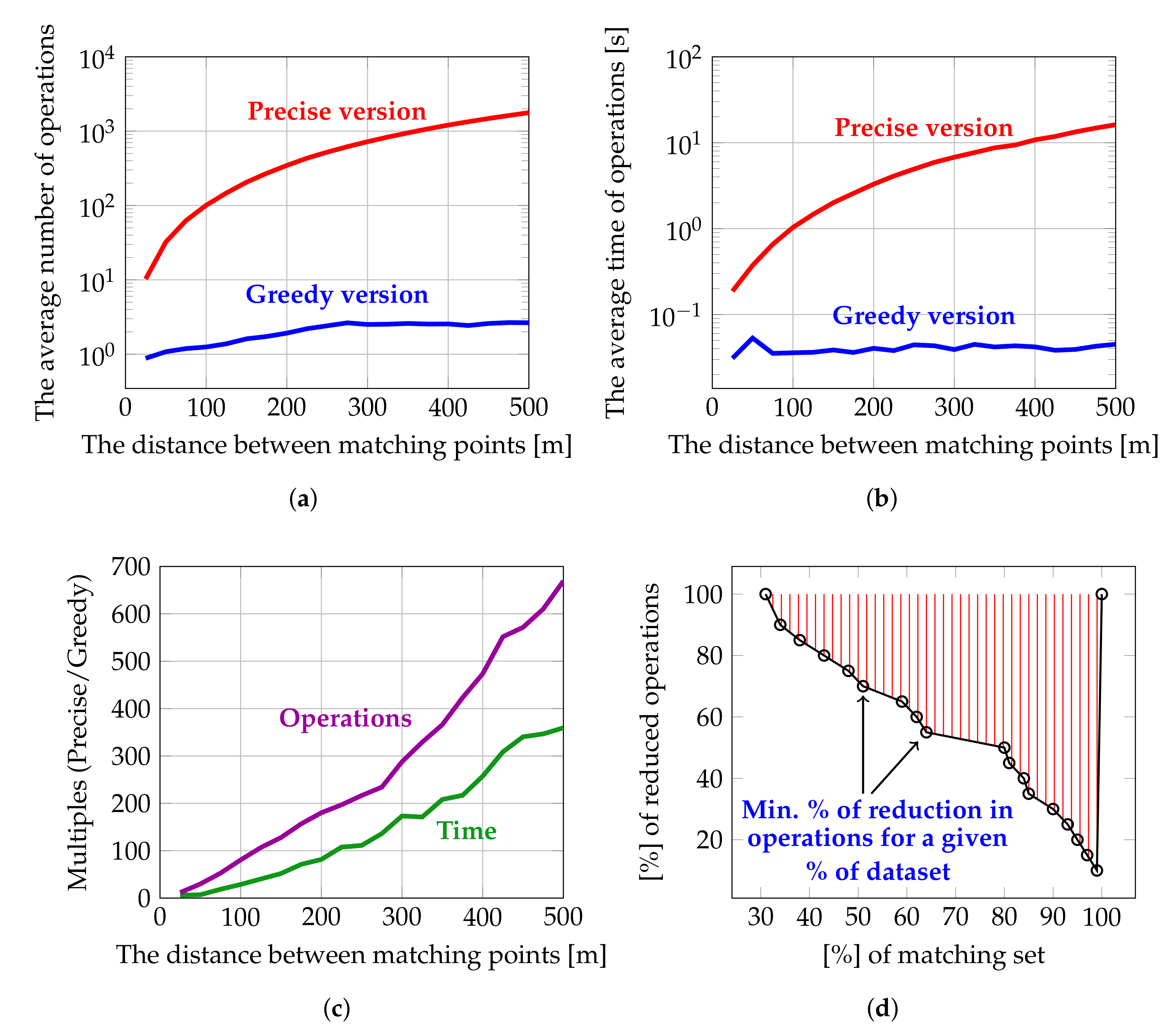
One of the differences between the precise and the greedy versions of the proposed algorithm is that, in the greedy version, the set of candidate Points of Interest does not include all those located within the given radius (in our case, 300 m). Instead, it includes only those POIs located in the given range whose Name is similar to the Name of the Point of Interest we are seeking matches for. Hence, the number of candidates is reduced in comparison to the precise version, and thus the number of potential operations (i.e., metrics calculations and classifications) is also reduced. Note that we used the term ’potential operations’ here, since, in the greedy version, candidates are sorted in descending order by Name similarity. Therefore, the chances are that the actual number of operations will be much lower, since the matching Point of Interest is often one of the first candidates from the sorted list. Figure 19a presents the average number of such potential operations as a function of matching point distance. Clearly, there is a great reduction in potential operations in favor of the greedy algorithm (from one order of magnitude for POIs with a distance close to 0, up to three orders of magnitude for POIs with distances between 400 and 500 m). One more important observation emerging from this chart is that, for the precise algorithm, the average number of potential operations noticeably increases as the distance between the matching points grows. In contrast, in the greedy version, this value is almost constant. In Figure 19b, we present the average time expended by both algorithm versions until the matching point was found. It shows that, in terms of computation time, on the ordinary PC employed in the tests with a 3.2 GHz quad-core Intel i5-4460 processor, 16 GB of RAM and 256 GB of solid-state storage, an advantage of two orders of magnitude can be observed for the greedy version. To make this contrast in results even more stark, the ratio between the number of potential operations to be performed by the precise and greedy versions for candidate Points of Interest located in the range of 0–500 m was calculated. The results are presented in Figure 19c (the violet line). Similarly, the ratio between the average time spent by the precise and greedy algorithms to find the matching point (for all considered distance ranges of 0–500 m) was calculated. The results are presented in Figure 19c (the green line). Finally, in Figure 19d, the correlation between the percentage of reduced operations and the number of matched pairs (i.e., how many pairs have reduced operations of at least X percent) is presented. It shows that, after sorting candidate POIs in descending order by Name similarity, for almost 31% of Points of Interest no additional operations were required. This is because the matching point was the first result from the sorted list, and for 80% of pairs, the number of operations was reduced by at least half.
The results confirm that modifications introduced into the greedy version are justified since, at a cost of just 3.5% in terms of accuracy, the time spent by the algorithm on Points of Interest matching was reduced by two orders of magnitude.
7. Conclusions and Future Work
The problem of matching POI objects arising from various sources is an emerging area of research. Although it is partially addressed in the literature, no comprehensive survey exists as yet. Moreover, the research that has been done thus far, was conducted on relatively small and disjunctive sets of data, making it difficult to draw comparisons and conclusions. In this paper, a comprehensive analysis is reported and an algorithm for automatic Points of Interest matching is proposed. For this purpose:
- We analyzed a selection of the most popular data sources—their structures, models, attributes, number of objects, the quality of data (number of missing attributes), etc. (see Section 3 for details).
- We defined the unified Point of Interest model and then implemented mappers for downloading data from different services and storing them in one, single, common model (see the first part of Section 3).
- We prepared a fairly large experimental dataset consisting of 50,000 matching and 50,000 non-matching points, taken from such diverse geographical, cultural and language areas as Liverpool, Beijing, and Ankara (see Section 3.2).
- We reviewed metrics that can be used for calculating the similarity between Points of Interest. For this, we analyzed three groups i.e., geographical distance, string similarity distance and semantic distance metrics (see Section 4.1).
- We verified four different strategies for dealing with missing attributes (see Section 4.2 for details).
- We reviewed and analyzed six different machine learning classifiers (k-Nearest neighbor, decision tree, random forest, isolation forest, and two neural net classifiers) for Points of Interest matching.
- We performed experiments and made comparisons taking into account different similarity metrics and different strategies for dealing with missing data (see Section 5.1 and Section 5.2 and Appendix A).
The combination of random forest algorithm with the marking of missing data and the mixing of different similarity metrics for different POI description attributes seems to be the best, and thus recommended, classifier for Points of Interest matching. Simultaneously, the best combination of POI attributes similarity metrics is using Token Set Ratio for POI Name, Token Sort Ratio for Address, Jaro–Winkler for Phone number, Ratio for WWW, and average of Wu–Palmer, Lin, and Path for POI category. With such a combination of classification algorithm, strategy for dealing with incomplete data and similarity metrics, the highest efficiency (95.2%) on a 100,000-POIs experimental dataset was achieved. This result is better than one of the best-known results as reported in [5], where the authors tested an Isolation Forest classifier coupled with the strategy.
Next, based on the results obtained in the analytical part of the research, an algorithm for automatic Points of Interest matching was proposed. First, we proposed an exact algorithm (see Algorithm 1) which works competently, but involves high computational complexity (for both the worst- and the average-case). Next, we proposed a slightly modified version (see Algorithm 2), characterized by the same worst-case complexity, but allowing for significant average complexity reduction (by as much as two orders of magnitude). Importantly, it achieved almost the same matching results (the value of the Accuracy metric deteriorated only by 3.5% in comparison to the precise version).
The next step in our work will be research into a hybrid classifier, which will apply the appropriate matching methods depending on the quality of the data provided. Subsequent work will also address the problem of applying the appropriate metrics depending on the geographical, cultural or language area the data come from (this particular problem was apparent in the results for Liverpool). We also intend to work on Full-Text Search instrumentation to address the problem reported at the end of Section 6. Solving these issues should bring us very close to a universal algorithm for automatic Points of Interest matching, one which will be completely independent of where the data are sourced from.
Author Contributions
Conceptualization, Mateusz Piech, Aleksander Smywinski-Pohl, Robert Marcjan, and Leszek Siwik; methodology, Mateusz Piech, Aleksander Smywinski-Pohl, Robert Marcjan, and Leszek Siwik; software, Mateusz Piech and Aleksander Smywinski-Pohl; validation, Aleksander Smywinski-Pohl, Robert Marcjan, and Leszek Siwik; formal analysis, Robert Marcjan and Aleksander Smywinski-Pohl; data preparation, Aleksander Smywinski-Pohl and Robert Marcjan; writing—original draft preparation, Mateusz Piech and Leszek Siwik; writing—review and editing, Leszek Siwik and Mateusz Piech; visualization, Leszek Siwik and Mateusz Piech; and supervision, Leszek Siwik and Robert Marcjan. All authors have read and agreed to the published version of the manuscript.
Funding
The research presented in this paper was supported by the funds of the Polish Ministry of Science and Higher Education assigned to AGH University of Science and Technology.
Conflicts of Interest
The authors declare no conflicts of interest.
Appendix A
Figure A1–Figure A5 show receiver operating characteristic curves, along with AUC values, obtained for the training set (100,000 POIs), for all considered distance metrics for all four considered strategies for handling missing data () for attributes Name, Address, Phone number, WWW, and Category.
Figure A1.
A receiver operating characteristics for all considered string similarity metrics for all four strategies for dealing with missing data for attribute Name.
Figure A1.
A receiver operating characteristics for all considered string similarity metrics for all four strategies for dealing with missing data for attribute Name.

Figure A2.
A receiver operating characteristics for all considered string similarity metrics for all four strategies for dealing with missing data for attribute Address.
Figure A2.
A receiver operating characteristics for all considered string similarity metrics for all four strategies for dealing with missing data for attribute Address.

Figure A3.
A receiver operating characteristics for all considered string similarity metrics for all four strategies for dealing with missing data for attribute Phone Number.
Figure A3.
A receiver operating characteristics for all considered string similarity metrics for all four strategies for dealing with missing data for attribute Phone Number.

Figure A4.
A receiver operating characteristics for all considered string similarity metrics for all four strategies for dealing with missing data for attribute Website.
Figure A4.
A receiver operating characteristics for all considered string similarity metrics for all four strategies for dealing with missing data for attribute Website.

Figure A5.
A receiver operating characteristics for all considered category similarity metrics for all four strategies for dealing with missing data for attribute Category.
Figure A5.
A receiver operating characteristics for all considered category similarity metrics for all four strategies for dealing with missing data for attribute Category.

References
- Scheffler, T.; Schirru, R.; Lehmann, P. Matching Points of Interest from Different Social Networking Sites. In Lecture Notes in Computer Science; Springer: Berlin/Heidelberg, Germany, 2012; pp. 245–248. [Google Scholar] [CrossRef]
- Yujian, L.; Bo, L. A Normalized Levenshtein Distance Metric. IEEE Trans. Pattern Anal. Mach. Intell. 2007, 29, 1091–1095. [Google Scholar] [CrossRef] [PubMed]
- McKenzie, G.; Janowicz, K.; Adams, B. A weighted multi-attribute method for matching user-generated Points of Interest. Cartogr. Geogr. Inf. Sci. 2014, 41, 125–137. [Google Scholar] [CrossRef]
- Novack, T.; Peters, R.; Zipf, A. Graph-Based Matching of Points-of-Interest from Collaborative Geo-Datasets. ISPRS Int. J. -Geo-Inf. 2018, 7, 117. [Google Scholar] [CrossRef] [Green Version]
- Almeida, A.; Alves, A.; Gomes, R. Automatic POI Matching Using an Outlier Detection Based Approach. In Advances in Intelligent Data Analysis XVII; Springer International Publishing: Berlin/Heidelberg, Germany, 2018; pp. 40–51. [Google Scholar] [CrossRef]
- Liu, F.T.; Ting, K.M.; Zhou, Z.H. Isolation Forest. In Proceedings of the 2008 Eighth IEEE International Conference on Data Mining, Pisa, Italy, 15–19 December 2008. [Google Scholar] [CrossRef]
- Factual Crosswalk API. Available online: https://www.factual.com/blog/crosswalk-api/ (accessed on 1 September 2019).
- Herzog, T.H.; Scheuren, F.; Winkler, W.E. Record linkage. WIREs Comput. Stat. 2010, 2, 535–543. [Google Scholar] [CrossRef]
- Li, L.; Xing, X.; Xia, H.; Huang, X. Entropy-weighted instance matching between different sourcing points of interest. Entropy 2016, 18, 45. [Google Scholar] [CrossRef] [Green Version]
- Kim, J.; Vasardani, M.; Winter, S. Similarity matching for integrating spatial information extracted from place descriptions. Int. J. Geogr. Inf. Sci. 2017, 31, 56–80. [Google Scholar] [CrossRef]
- Deng, Y.; Luo, A.; Liu, J.; Wang, Y. Point of Interest Matching between Different Geospatial Datasets. ISPRS Int. J. Geo-Inf. 2019, 8, 435. [Google Scholar] [CrossRef] [Green Version]
- Haklay, M. How good is volunteered geographical information? A comparative study of OpenStreetMap and Ordnance Survey datasets. Environ. Plan. B Plan. Des. 2010, 37, 682–703. [Google Scholar] [CrossRef] [Green Version]
- Hochmair, H.H.; Juhász, L.; Cvetojevic, S. Data quality of points of interest in selected mapping and social media platforms. In Proceedings of the LBS 2018: 14th International Conference on Location Based Services, Zurich, Switzerland, 15–17 January 2018; pp. 293–313. [Google Scholar]
- Auer, S.; Bizer, C.; Kobilarov, G.; Lehmann, J.; Cyganiak, R.; Ives, Z. Dbpedia: A nucleus for a web of open data. In The Semantic Web; Springer: Berlin/Heidelberg, Germany, 2007; pp. 722–735. [Google Scholar]
- OpenStreetMap TagInfo. Available online: https://taginfo.openstreetmap.org/ (accessed on 1 September 2019).
- OpenStreetMap Wiki. Available online: https://wiki.openstreetmap.org/ (accessed on 1 September 2019).
- Cohen, W.W.; Ravikumar, P.; Fienberg, S.E. A Comparison of String Metrics for Matching Names and Records. In Proceedings of the KDD Workshop On Data Cleaning and Object Consolidation, Washington, DC, USA, 24–27 August 2003. [Google Scholar]
- FuzzyWuzzy: Fuzzy String Matching in Python. Available online: https://chairnerd.seatgeek.com/fuzzywuzzy-fuzzy-string-matching-in-python/ (accessed on 1 September 2019).
- Blanchard, E.; Harzallah, M.; Briand, H.; Kuntz, P. A Typology of Ontology-Based Semantic Measures. In Proceedings of the EMOI-INTEROP 2005, Porto, Portugal, 13–14 June 2005; Volume 160. [Google Scholar]
- Fix, E.; Hodges, J.L., Jr. Discriminatory Analysis-Nonparametric Discrimination: Consistency Properties; Technical Report; University of California: Berkeley, CA, USA, 1951. [Google Scholar]
- Pedregosa, F.; Varoquaux, G.; Gramfort, A.; Michel, V.; Thirion, B.; Grisel, O.; Blondel, M.; Prettenhofer, P.; Weiss, R.; Dubourg, V.; et al. Scikit-learn: Machine learning in Python. J. Mach. Learn. Res. 2011, 12, 2825–2830. [Google Scholar]
- Quinlan, J.R. Induction of decision trees. Mach. Learn. 1986, 1, 81–106. [Google Scholar] [CrossRef] [Green Version]
- Breiman, L. Random forests. Mach. Learn. 2001, 45, 5–32. [Google Scholar] [CrossRef] [Green Version]
- Zhang, G.P. Neural networks for classification: A survey. IEEE Trans. Syst. Man Cybern. Part C Appl. Rev. 2000, 30, 451–462. [Google Scholar] [CrossRef] [Green Version]
- Abadi, M.; Barham, P.; Chen, J.; Chen, Z.; Davis, A.; Dean, J.; Devin, M.; Ghemawat, S.; Irving, G.; Isard, M.; et al. Tensorflow: A system for large-scale machine learning. In Proceedings of the 12th {USENIX} Symposium on Operating Systems Design and Implementation ({OSDI} 16), Savannah, GA, USA, 2–4 November 2016; pp. 265–283. [Google Scholar]
- Keras: The Python Deep Learning library. Available online: https://keras.io/ (accessed on 1 September 2019).
- Fawcett, T. An introduction to ROC analysis. Pattern Recognit. Lett. 2006, 27, 861–874. [Google Scholar] [CrossRef]
- August, P.; Michaud, J.; Labash, C.; Smith, C. GPS for environmental applications: Accuracy and precision of locational data. Photogramm. Eng. Remote Sens. 1994, 60, 41–45. [Google Scholar]
Figure 1.
The JSON-structured (parts of) Point of Interest models of: FourSquare (a); Yelp (b); Facebook Places (c); and OpenStreetMap (d).
Figure 1.
The JSON-structured (parts of) Point of Interest models of: FourSquare (a); Yelp (b); Facebook Places (c); and OpenStreetMap (d).
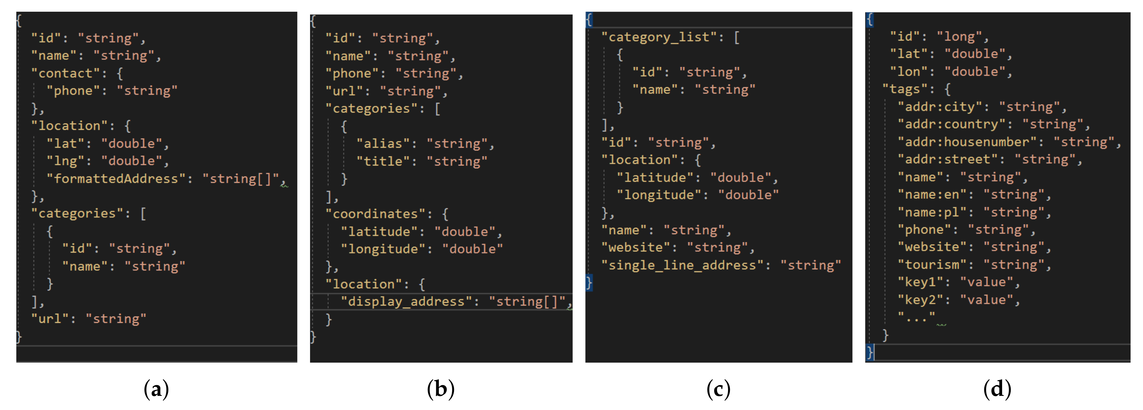
Figure 2.
Unified Point of Interest model presented as a UML diagram.
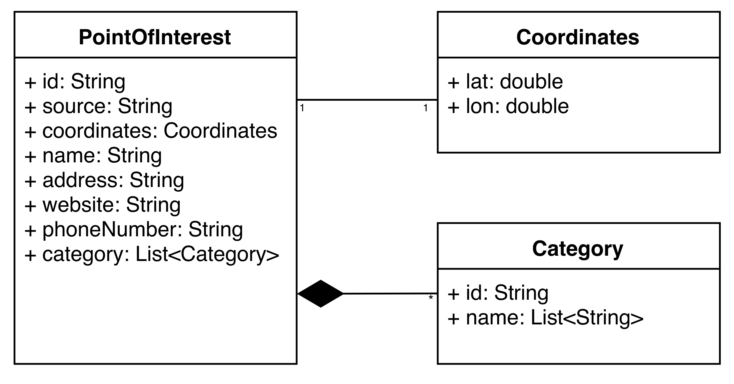
Figure 3.
Cities used for training (red markers) and verifying (green markers) datasets.

Figure 4.
The percentage of missing attributes in training and test sets.

Figure 5.
OpenStreetMap: The percentage of POIs with 0–4 missing attributes (a); and the percentage of completeness of selected attributes (b).
Figure 5.
OpenStreetMap: The percentage of POIs with 0–4 missing attributes (a); and the percentage of completeness of selected attributes (b).

Figure 6.
Foursquare: The percentage of POIs with 0–4 missing attributes (a); and the percentage of completeness of selected attributes (b).
Figure 6.
Foursquare: The percentage of POIs with 0–4 missing attributes (a); and the percentage of completeness of selected attributes (b).
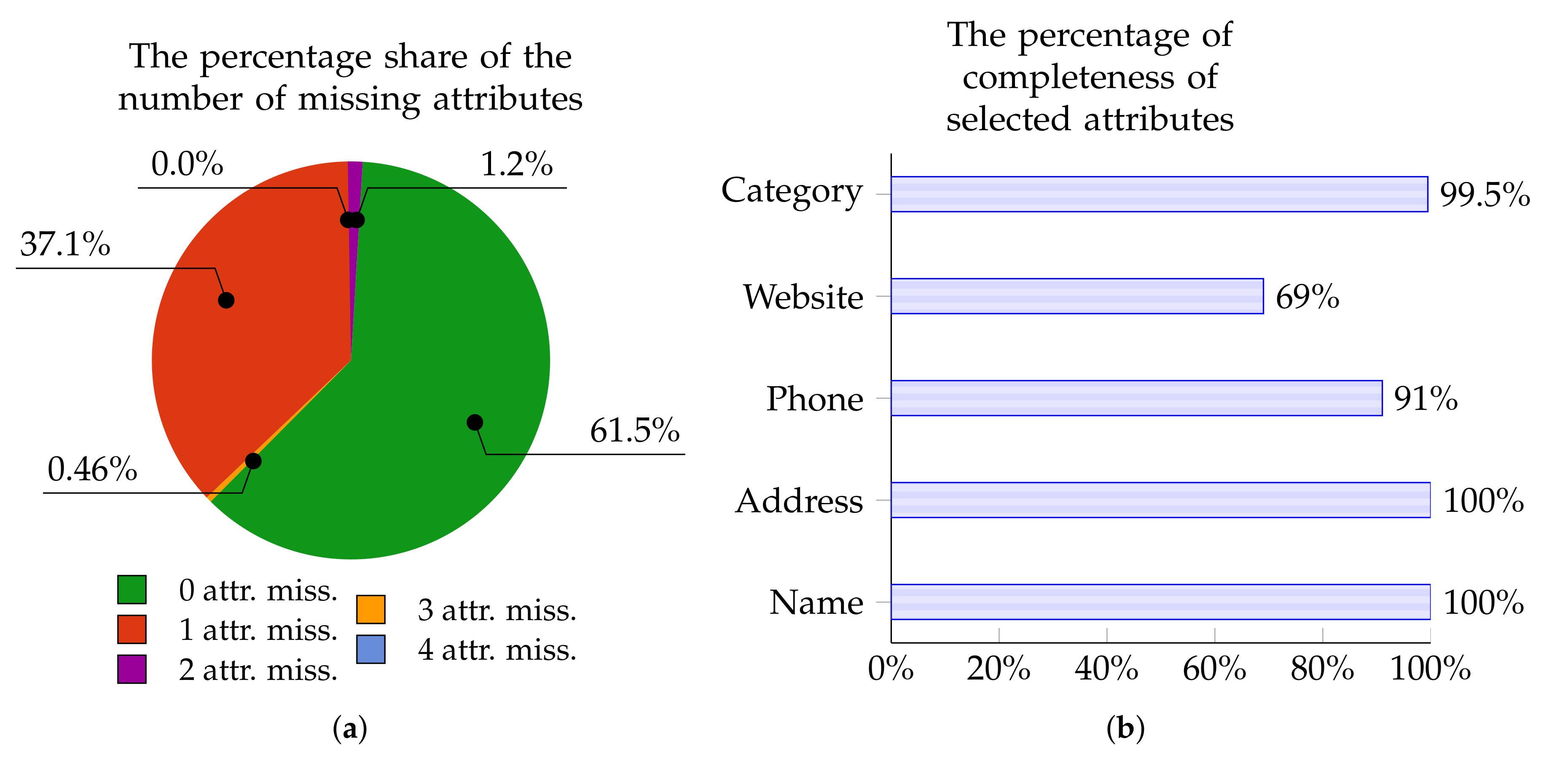
Figure 7.
Facebook Places: The percentage of POIs with 0–4 missing attributes (a); and the percentage of completeness of selected attributes (b).
Figure 7.
Facebook Places: The percentage of POIs with 0–4 missing attributes (a); and the percentage of completeness of selected attributes (b).

Figure 8.
Yelp: The percentage of POIs with 0–4 missing attributes (a); and the percentage of completeness of selected attributes (b).
Figure 8.
Yelp: The percentage of POIs with 0–4 missing attributes (a); and the percentage of completeness of selected attributes (b).

Figure 9.
The percentage of matching POIs within the range of 0–300 m (a); and for the sub-range of 200–300 m (b).
Figure 9.
The percentage of matching POIs within the range of 0–300 m (a); and for the sub-range of 200–300 m (b).

Figure 10.
The distribution of in the training set for matched and mismatched POIs.

Figure 11.
Receiver operating characteristics for coordinates.

Figure 12.
The best AUC values (b) and best ROC curves characteristics (a) for attribute Name.

Figure 13.
The best AUC values (b) and best ROC curves characteristics (a) for attribute Address.

Figure 14.
The best AUC values (b) and best ROC curves characteristics (a) for attribute Phone Number.
Figure 14.
The best AUC values (b) and best ROC curves characteristics (a) for attribute Phone Number.

Figure 15.
The best: AUC values (b) and ROC curves characteristics (a) for attribute WWW.

Figure 16.
The best AUC values (b) and best ROC curves characteristics (a) for combination of attributes.
Figure 16.
The best AUC values (b) and best ROC curves characteristics (a) for combination of attributes.

Figure 17.
The best AUC values (b) and best ROC curves characteristics (a) for attribute Category.

Figure 18.
Receiver operating characteristics for all attributes.

Figure 19.
The average number of operations to be performed by the precise and greedy algorithm versions as a function of matching point distance (a); the average time of operations performed by the precise and greedy algorithm versions as a function of matching point distance (b); the ratios of the number of operations and time (c); and the minimum percentage of reduced operations for the given percentage of POIs in the validation set (d).


Table 1.
Comparison of the values of the analyzed metrics for sample strings.
| Henryka Kamienskiego 11 Krakow Polska | Generala Henryka Kamienskiego 30-644 Krakow | 0.49 | 0.70 | 0.70 | 0.79 | 0.83 | 1.0 | 0.81 |
| Pokoju 44, 31-564 Krakow | Zakopianska 62 Krakow Polska | 0.25 | 0.51 | 0.42 | 0.46 | 0.55 | 1.0 | 0.51 |
| Cinema City Poland | Cinema City | 0.61 | 0.92 | 0.76 | 1.0 | 1.0 | 1.0 | 1.0 |
| 786934146 | 48786934146 | 0.75 | 0.81 | 0.86 | 1.0 | 1.0 | 1.0 | 1.0 |
| http://bestwestern\krakow.pl/en/ | http://bestwestern\krakow.pl/ | 0.88 | 0.98 | 0.93 | 1.0 | 0.90 | 1.0 | 0.95 |
Table 2.
The best accuracy values for different classification algorithms.
| Strategy | K-Neigh | Dec Tree | Rnd Forest | Isol Forest | Perceptron | FF Net |
|---|---|---|---|---|---|---|
| 97.6% | 95.9% | 97.6% | 95.3% | 93.2% | 98.2% | |
| 92.8% | 91.7% | 95.1% | 74.5% | 76.5% | 87.4% | |
| 92.0% | 95.1% | 95.2% | 91.6% | 89.7% | 91.2% | |
| 54.1% | 35.8% | 33.2% | 93.4% | 56.7% | 60.0% |
Table 3.
The best AUC and score values for selected cities.
| City | AUC | Score |
|---|---|---|
| Krakow | 99.5% | 99.4% |
| San Francisco | 92.4% | 92.2% |
| Naples | 93.8% | 92.8% |
| Liverpool | 84.0% | 83.5% |
| Beijing | 98.1% | 91.3% |
Table 4.
A comparison of the precise and greedy versions of the algorithm for automatic Points of Interest matching run on the validation set.
Table 4.
A comparison of the precise and greedy versions of the algorithm for automatic Points of Interest matching run on the validation set.
| Precise Algorithm | Greedy Algorithm | |
|---|---|---|
| Accuracy | 84.73% | 81.23% |
| Matches not found | 0% | 11.52% |
| Invalid matches | 15.27% | 7.25% |
Table 5.
The number of operations performed by the precise and greedy versions of the automatic POIs matching algorithm.
Table 5.
The number of operations performed by the precise and greedy versions of the automatic POIs matching algorithm.
| Precise Algorithm | Greedy Algorithm | % of Reduced Classifications | |
|---|---|---|---|
| Number of classifications required for 20,000 matching and non-matching cases | 69,783 | 29,979 | 57% |
| Number of classifications required for 7000 matching cases | 63,928 | 24,124 | 62% |
© 2020 by the authors. Licensee MDPI, Basel, Switzerland. This article is an open access article distributed under the terms and conditions of the Creative Commons Attribution (CC BY) license (http://creativecommons.org/licenses/by/4.0/).
Share and Cite
MDPI and ACS Style
Piech, M.; Smywinski-Pohl, A.; Marcjan, R.; Siwik, L. Towards Automatic Points of Interest Matching. ISPRS Int. J. Geo-Inf. 2020, 9, 291. https://0-doi-org.brum.beds.ac.uk/10.3390/ijgi9050291
AMA Style
Piech M, Smywinski-Pohl A, Marcjan R, Siwik L. Towards Automatic Points of Interest Matching. ISPRS International Journal of Geo-Information. 2020; 9(5):291. https://0-doi-org.brum.beds.ac.uk/10.3390/ijgi9050291
Chicago/Turabian StylePiech, Mateusz, Aleksander Smywinski-Pohl, Robert Marcjan, and Leszek Siwik. 2020. "Towards Automatic Points of Interest Matching" ISPRS International Journal of Geo-Information 9, no. 5: 291. https://0-doi-org.brum.beds.ac.uk/10.3390/ijgi9050291
Note that from the first issue of 2016, this journal uses article numbers instead of page numbers. See further details here.