A Neural Networks Approach to Detecting Lost Heritage in Historical Video

Abstract

Documenting Cultural Heritage through the extraction of 3D measures with photogrammetry is fundamental for the conservation of the memory of the past. However, when the heritage has been lost the only way to recover this information is the use of historical images from archives. The aim of this study is to experiment with new ways to search for architectural heritage in video material and to save the effort of the operator in the archive in terms of efficiency and time. A workflow is proposed to automatically detect lost heritage in film footage using Deep Learning to find suitable images to process with photogrammetry for its 3D virtual reconstruction. The performance of the network was tested on two case studies considering different architectural scenarios, the Tour Saint Jacques which still exists for the tuning of the networks, and Les Halles to test the algorithms on a real case of an architecture which has been destroyed. Despite the poor quantity and low quality of the historical images available for the training of the network, it has been demonstrated that, with few frames, it was possible to reach the same results in terms of performance of a network trained on a large dataset. Moreover, with the introduction of new metrics based on time intervals the measure of the real time saving in terms of human effort was achieved. These findings represent an important innovation in the documentation of destroyed monuments and open new ways to recover information about the past.

1. Introduction

The documentation of Cultural Heritage plays a critical role in the conservation of memory and knowledge of the past, and both are necessary to make the best decisions for its protection. An important aspect of the documentation process concerns the collection of data and information about heritage. For this reason, recent research in this field has seen the rapid development of technologies to support the management and analysis of historical data regarding heritage. With Machine Learning (ML), tasks like the processing of these great amounts of data and the reduction of human effort can be made automatic and therefore more efficient. If Artificial Intelligence (AI) is combined with techniques widely used in the heritage field such as photogrammetry, the documentation process can really be improved, as demonstrated in this paper.

This research focuses on the examination of historical archive data, considering historical film footage in particular. The importance of these multimedia materials lies in the fact that heritage monuments and parts of a city that are no longer existing appear in them. For this reason, when there are no other ways to document the lost heritage, these data become sources of key importance, from a cultural and architectural point of view. However, an important issue regarding historical images concerns their availability and accessibility in archives, often made difficult by the lack of an appropriate organization of these data. From a photogrammetric point of view, it is very difficult to process historical material, because even if it was not acquired for this purpose, it has properties that make it difficult to use in conventional photogrammetric workflows, such as poor image quality, complete lack of camera parameters, the presence of distortion and damage due to poor storage. The main disadvantage of historical film footage is that it was not shot for use in 3D reconstruction. Information on camera type, camera movement and film used is not always available.

This study intends to determine how to improve ways to search for architectural heritage in video material and to reduce the effort of the operator in the archive in terms of efficiency and time. In order to achieve this goal, a workflow is proposed to automatically detect lost heritage in film footage and its three-dimensional virtual reconstruction. Starting from the standard photogrammetric pipeline, two new steps were added by the authors. The first one concerned the retrieval of suitable images to process with photogrammetry using Deep Learning (DL) for the automatic recognition of heritage in the film footage. The second one was the validation of photogrammetric reconstruction through the metric quality assessment of the model obtained.

This paper is divided into four parts. In the first part the state of the art of DL applied to Cultural Heritage is presented and the open issues in collecting historical material are identified. The second part describes the methodology used for testing the workflow and the metrics used to evaluate it, both standard and new. Two parallel case studies are presented in the third part, focusing on the collection and preparation of the datasets. Finally, the fourth part analyses the performance of the networks implemented and discusses the results on real cases, highlighting the efficiency of the experimented workflow to test for the time and effort saved in the work of the final user.

2. State of the Art: Artificial Intelligence for Cultural Heritage

In recent years, there has been an increasing interest in the digitalization of Cultural Heritage collections. Thanks to the launch of large campaigns of digitization by several institutional and private entities, billions of documents are now available through online tools. Creating new tools for the final user of these data is an appealing research topic especially in the AI domain. In fact, the volume, the size and the variety of historical data lead to some critical factors. The most important is concerned the manpower needed to organize and search the documents. To solve this problem the application of Machine Learning gives opportunities to enhance historical archives and retrieval of heritage information.

Machine Learning technique has become fundamental not only in the field of computer science research, but also in everyday life, finding applications for example in web search engines, fraud detection systems, spam filters, automatic text analysis systems, and medical diagnostic systems. One of the reasons for this growing importance is the successful application of DL methods in areas such as image classification [1,2,3], in which convolutional neural networks (CNNs) exceed the human level in object recognition and image search [4,5]. However only a few studies in Cultural Heritage have developed in this area. So far, thanks to this approach, researchers have been able to classify interesting objects in images of buildings of architectural value [6]; identify different monuments based on the feature of the images of monuments [7]; automatically annotate the cultural assets based on their visual feature and the available metadata [8]; recognize a character in images of artworks and their contexts [9]; interpret deep features learned by Convolutional Neural Networks for city recognition [10].

Besides the improvements of Machine Learning techniques, hardware development, in particular the use of Graphical Processing Units (GPUs), has given a boost to the computational efficiency of such algorithms.

Existing research recognizes the important role played by historical data in archives and the potentialities of ML and proposed different methods: to automatically index and label the documents and search through the collections [11]; to retrieve images and information on heritage [12] and iconographic contents representing landscapes of the French territory [13]. However, the majority of these works that consider the analysis of paintings, drawings, images, and film footage have been hardly explored with these techniques. Only an example of Deep Learning application to extract semantic features to analyze the role of intertitles in early cinema was conducted [14].

The reason is that, among the historical material, the collection of film footage is linked by some specific critical factors. One limitation is represented by the difficulty of finding the material which often requires physical access to the archives, which in many cases allow on-site consultation but not data sharing. In this regard, the development of international projects (such as iMediaCities [15]) aimed at limiting the barriers to access to data in video archives deserves special attention. Another problem is the need to identify the object of interest within the amount of material that potentially contains it. The indexing of metadata for historical archival material is often incomplete or inaccurate, and the corresponding search engines are therefore not very efficient. The human effort to find the data of interest represents a significant percentage of the final user work.

These problems were initially addressed in [16] in which the first experiments on the use of Neural Networks for the recognition of architectures in films were carried out. In this paper the application of the workflow was extended in many respects, i.e., considering new experiments on real cases of Cultural Heritage that no longer exist, investigating the quality and quantity of training datasets, and proposing new metrics more oriented to the final user gain.

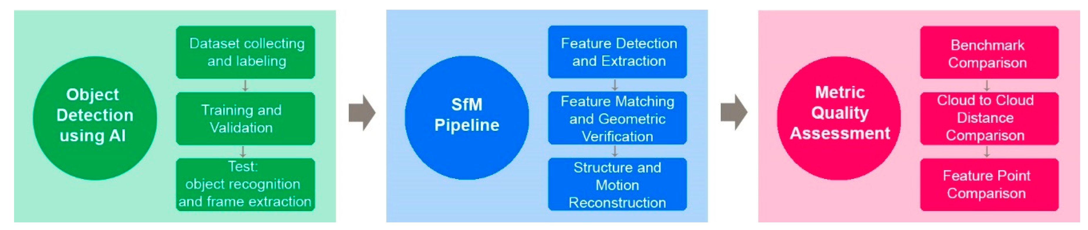
3. Proposed Workflow

In the workflow proposed in this paper a combination of DL techniques with photogrammetry is presented. DL is used for the retrieval of primary data used as input material in the standard Structure-from-Motion (SfM) pipeline.

In order to allow a better assessment of the validity of the pipeline, an additional validation step of metric quality evaluation of the point cloud obtained concludes the workflow.

COLMAP [17] open-source Structure-from-Motion and Multi-View Stereo (MVS) algorithm implementation, developed by ETH of Zurich [18], is the pipeline chosen as the reference in this work.

This software is designed to create a versatile incremental SfM system for the reconstruction of collections of unordered photographs. The use of open-source algorithms allows the control of the quality of the results at each stage of the photogrammetric pipeline and avoids the blind automatisms of commercial software packages. The current state-of-the-art SfM algorithms fail to capture images with low overlap, poor resolution and missing metadata, and deliver fully satisfactory results in terms of completeness and robustness. The advantage of COLMAP is that the accuracy of the results is significantly improved while increasing efficiency at every stage of incremental reconstruction. Moreover, it allows the setting of a suitable scenario for video sequences.

Figure 1 shows the workflow in which the standard photogrammetric process is modified with the object detection phase in the first part and the metric quality assessment in the last part.

3.1. Object Detection Using Neural Networks

The first part of the workflow is concerning the use of Neural Networks (NN) intending to detect the object of interest in the film footage. Among the different types available, Neural Networks that support the Object detection algorithm were chosen. This solution was indeed effective for the experimented pipeline since it allows image classification even in complex images and with the extraction of bounding boxes of the object recognized.

The usability of the workflow from the operator in the archive is an important aspect to consider. For this reason, the Luminoth software [19] based on TensorFlow [20] was selected because it implements an object detection algorithm through state-of-the-art networks. In particular, in this work the following networks were used:

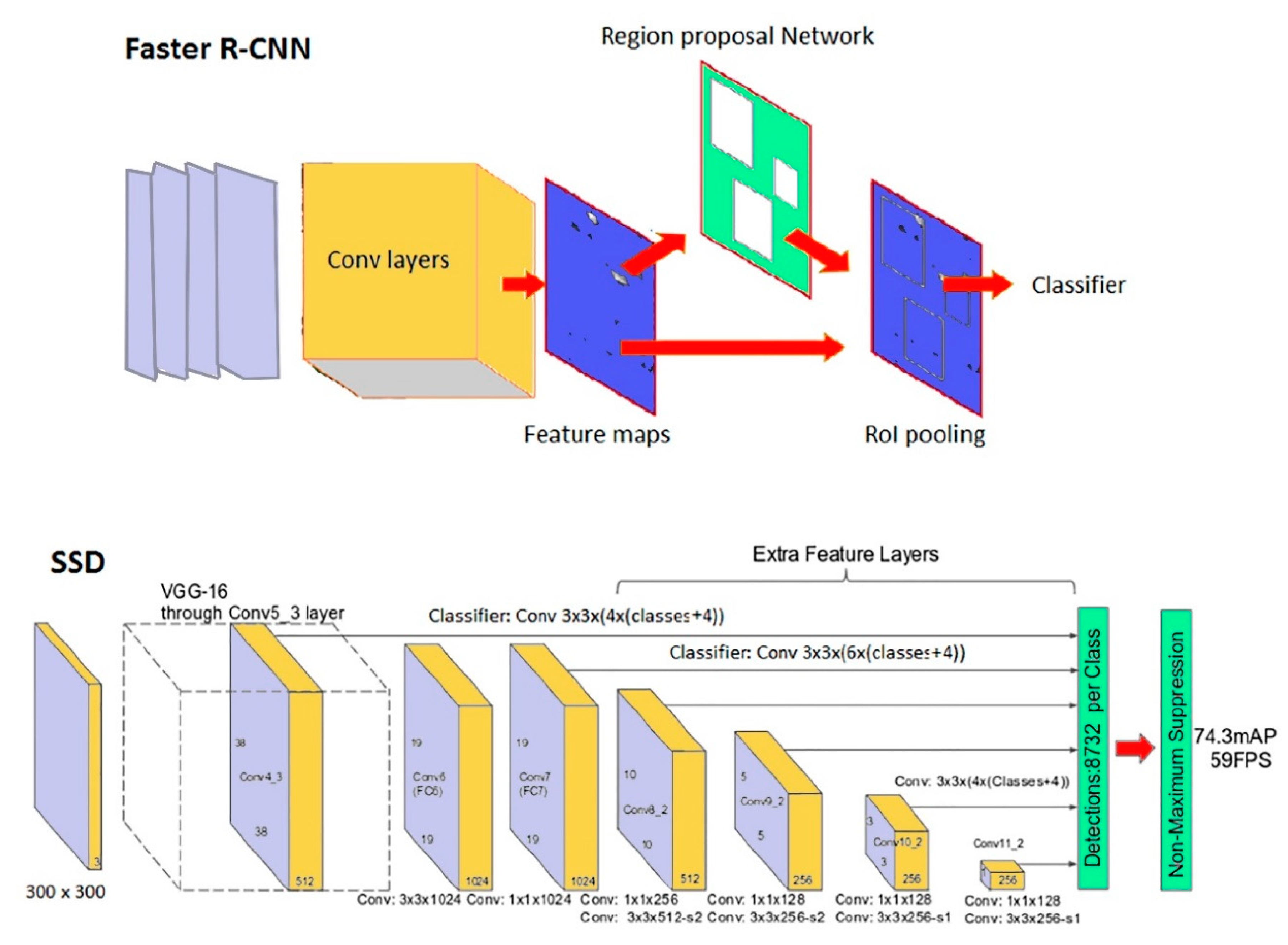
• Faster R-CNN [21]: stands for Faster Region-based Convolutional Neural Network and it is the evolution of an R-CNN network [22] whose purpose is to reduce the object detection problem to a classification problem made on limited regions of an image. The idea behind this type of network is very simple: sub-portions of an image (regions) are selected and these regions are used as the input of a classifier that uses convolution networks to determine the class of the extracted object. From the computational point of view, it would not be possible to apply the classifier to every possible sub-image of the starting image; for this reason R-CNN was designed to reduce the number of possible regions to be used by the classifier. The R-CNN network uses an algorithm for selecting possible regions (region-proposal) which reduces, around 2000 times, the number of images fed to the classifier. For each proposed region, the classifier that determines the class of the region is applied; and possibly a regression over a set of bounding boxes is applied to determine the optimal bounding box of the region containing the object. For the selection of the region module, a variety of methods for generating category-independent region proposals exist. The main aspect of the Faster R-CNN network is the replacement of the region selection algorithm (a computationally expensive part) with a convolutional network called the Region Proposal Network. The result is a network hundreds of times faster than the I R-CNN but with a comparable accuracy. A simplified sketch of the Faster R-CNN network is provided in Figure 2.
• SSD [23]: stands for Single Shot Detector and it is oriented to reduced computational demand while keeping an adequate accuracy. The SSD model is simpler if compared to methods that require object proposals because it completely eliminates proposal generation and subsequent pixel or feature resampling stage and encapsulates all computation in a single network. The network allows to discretize the output space of bounding boxes into a set of default boxes over different aspect ratios and scales per feature map location. At prediction time, the network generates scores for the presence of each object category in each default box and produces adjustments to the box to better match the object shape. A simplified sketch of the SSD network is provided in Figure 2. As a general rule, SSD networks are usually expected to be faster but less accurate than Faster R-CNN networks. This behavior, however, depends on the sizes of the considered objects and other factors, and it will be discussed in Section 5 of this paper in the context of investigated Cultural Heritage cases.

The described networks are provided already pre-trained by Luminoth. However, it is possible to add a new element to detect with a further training phase. This point is particularly important for the Cultural Heritage field because specific training is a necessary step.

From a user perspective, data preparation can also be a critical issue. The tool VGG Image Annotator (VIA) has been used for the annotation of the bounding box of the architectural heritage. VIA is a simple and standalone manual annotation tool for images, audio and video that allows the description of spatial regions in images or video frames. These manual annotations can be exported to plain text data formats such as JSON and CSV and therefore are ready for further processing by other software tools [24].

The file with the bounding box coordinates was used to prepare the dataset according to the requirements of Luminoth. After that, a configuration file has to be created specifying some necessary information, such as a run name, the location of the dataset and the model to use to train the network.

Luminoth also allows users to select the hyperparameters of the training, i.e., the parameters whose values are used to control the learning process. The selection is performed by manually customizing the training configuration file. Tuning the hyperparameters can be crucial to optimally solve the machine learning problem, e.g., in terms of convergence, stability and performance of training and inference phases. All in all, the default values provided by Luminoth mostly demonstrated to be effective in terms of all of the objectives. In particular, the momentum optimizer [25] was adequate to reach convergence. As for the learning rate tuning, the default values were usually adequate but for some SSD-based training runs, some convergence issues arose, and these problems were addressed by modifying the learning rate value from the default (0.0003) to lower values (e.g., 0.00006). Luminoth also integrates an automatic data augmentation mechanism and it was helpful to increase the entropy of data used in the training. As concerns the number of epochs to be used during the training, it was manually selected to ensure a complete training convergence. An early stopping mechanism might be possible but it was not attempted so far to always get the best results for the considered test cases. Finally, in the Section 5 of this work, an analysis of computing time performances comparing different generations of hardware is provided to complete the picture also from that point of view.

Evaluation Metrics of Neural Networks

As introduced, the NNs potentially improve the efficiency of the first part of the photogrammetric workflow. However, it is necessary to evaluate this performance more objectively, directly addressing also the efficiency and reliability of the algorithm in reducing the effort of the final user activity. According to these considerations, two different types of metrics evaluation of the network are considered in this paper. In the first type, the efficiency of the performance of NN is evaluated using standard metrics based on images or frames evaluated separately, while in the second type of evaluation the metrics are more closely related to the final tasks of the network, i.e., discovering the time intervals where a selected object appears in a video minimizing the human time required to manually analyze the movies. According to the frame-based approach, standard conventions can be followed: given a dataset of images, it is first defined P (N) as the number of images in which the object is present (not present), respectively. During the real-world inference phase, these values are not known, and the network output is P’ (N’) that represents the images in which the network has found (not found) the object. When performing the object detection inference, a probability of the presence of the object is typically returned. Therefore, in order to get the P’ and N’ values, it is necessary to define a probability threshold which is the minimum probability to be returned to consider the object as found. In order to validate the network performances, a test phase in which P and N are known is taken in consideration so that it is possible to categorize the images according to four statuses: True Positive (TP, image in both P a‘d P ’), True Negative (TN, image both in N and ‘n N ’), False Positive (FP, image’in P’ but not in P) and False Negative (FN, image ‘n N ’but not in N). Obviously, T=TP+FN and N=TN+FP. Such quantities can be combined to define meaningful parameters. In particular, a typical indicator is the accuracy, calculated as:

$$\mathrm{AC}=\frac{\mathrm{TP}+\mathrm{T}}{\mathrm{TP}+\mathrm{TN}+\mathrm{FP}+\mathrm{FN}}$$

(1)

Two other typical indicators are:

• Sensitivity (SN): defined as the number of correct positive predictions divided by the total number of positives:

  $$\mathrm{SN}=\frac{\mathrm{TP}}{\mathrm{TP}+\mathrm{FN}}$$

  (2)
• Specificity (SP): defined as the number of correct negative predictions divided by the total number of negatives:

  $$\mathrm{SP}=\frac{\mathrm{TN}}{\mathrm{TN}+\mathrm{FP}}$$

  (3)

Considering a set of test images composed only of positive (negative) images, it is clear that TN = FP = 0 (TP = FN = 0) and the accuracy exactly corresponds to the sensitivity (specificity). As detailed in the next section, considering positive-only (or negative-only) sets is very useful during the network training and validation phase to evaluate different capabilities of the network.

The indicators above are useful because they can work with both images and video frames, allowing fine-grained comparisons, and are especially useful to assess the quality of the network during the training phase. However, considering the usage of the network in a real-world context, where a certain object has to be detected from a large number of video archives, the authors believe that a set of metrics based on the time intervals is more suitable to summarize the advantages of using NNs in preference to the manual alternative. Referring these measures to the intervals is more natural if we consider that once a time interval with the searched object is found also with a single-frame, it is easy to identify the correct time set in which the monument appeared simply by going back or forward in the video. The proposed metrics are, therefore:

● Discovery Rate (DR): calculated as the number of the intervals correctly predicted by the network divided by the total number of the true intervals:

$$\mathrm{DR}=\frac{\mathrm{TP}\left(\mathrm{n}.\mathrm{correctly}\mathrm{predicted}\mathrm{intervals}\right)}{\mathrm{P}\left(\mathrm{n}.\mathrm{correctly}\mathrm{true}\mathrm{intervals}\right)}$$

(4)

A time interval in which the searched object appears is considered “correctly predicted” if there is a predicted interval that overlaps with the true interval for at least 1 s of video. This discovery rate is somehow related to the sensitivity; indeed, it indicates a measure of the correct positive predictions over the total number of positive cases. This metric describes an issue that is very important for the user, i.e., the capacity of the network to detect monuments avoiding loss of information.

● Time save Rate (TSR): calculated as the total time length of the video divided by the sum of the times of the measured intervals:

$$\mathrm{TSR}=\frac{\mathrm{Total}\mathrm{video}\mathrm{length}}{\mathrm{Sum}.\mathrm{times}\mathrm{of}\mathrm{predicted}\mathrm{intervals}}$$

(5)

This parameter is somehow related to the specificity and indicates how much time the operator would save in his manual work of watching videos if the automatism of the network is used. This parameter clearly depends also on the type of videos used for testing. The vast majority of the results presented in this paper are based on videos which contain at least one occurrence of the searched object, such a circumstance artificially limits the measured time save rate. To circumvent the dependency on the archive source, another time save related parameter is defined.

● Time save Efficiency (TSE): as said, the time save rate indicates the quantitative advantage for the end-user who adopts NN. It would be interesting to compare the time save rate with the ideal time save rate, which is the minimum time save rate knowing in advance the true intervals to watch. The ratio between the measured time save and the ideal time save rate is the time save efficiency:

$$\begin{array}{ll}\mathrm{TSE}& =\frac{\mathrm{TSR}\mathrm{measured}}{\mathrm{TSR}\mathrm{ideal}}=\frac{\raisebox{1ex}{$\mathrm{Total}\mathrm{video}\mathrm{length}$}\!\left/ \!\raisebox{-1ex}{$\mathrm{Sum}.\mathrm{times}\mathrm{of}\mathrm{predicted}\mathrm{intervals}$}\right.}{\raisebox{1ex}{$\mathrm{Total}\mathrm{video}\mathrm{length}$}\!\left/ \!\raisebox{-1ex}{$\mathrm{Sum}.\mathrm{times}\mathrm{of}\mathrm{true}\mathrm{intervals}$}\right.}\\ & =\frac{\mathrm{Sum}.\mathrm{times}\mathrm{of}\mathrm{true}\mathrm{intervals}}{\mathrm{Sum}.\mathrm{times}}\end{array}$$

(6)

The time save efficiency is less prone to bias due to the type of archive source. The value of this efficiency is typically reduced when dealing with false positives, i.e., when some measured intervals do not correspond to true intervals. However, it is worth noting that this efficiency can also reach values greater than 1 and this can happen when not all the true intervals are correctly found by the measured intervals. In this scenario, despite the false-positive intervals, it is possible that the total time of the measured intervals becomes shorter than the time of true intervals. However, this is a clear symptom of a poor discovery rate.

In general, discovery-rate, time save rate, and time save efficiency should all be maximized to improve training but, when it is not possible, the choice of one metric or another is a matter of usage context. Because of the type of use of the network within the photogrammetric pipeline, two extreme cases of use are considered:

• In the first situation in which the videos selected by the ML are then manually watched to decide which are the most suitable for photogrammetry, it is ideal to maximize the discovery rate to avoid losing useful information.
• In the second situation in which the pipeline is managed more automatically, it is instead preferable to maximize the time save parameters to prevent incorrect images from entering the subsequent processing.

3.2. SfM Pipeline Using COLMAP

In the second part of the workflow, the photogrammetric processing was implemented according to the standard principal steps. The first one is the detection and extraction of the feature in the frame extracted from the video that contains the heritage. During this phase, a camera model suitable to control the distortion effects was chosen, due to the lack of knowledge of the intrinsic parameter. The model considered five parameters, f for the focal length, cx and cy for the two coordinates of the principal point and k1 and k2 as the two radial distortion parameters. The second step is the feature matching of sequential images such as those obtained from a video and during this phase consecutive frames with visual overlap were matched. The last step of the reconstruction of the 3D model allowed the achievement of the final point cloud.

The last part of the workflow consisted of the evaluation of the metric quality of this model. In order to analyze the precision of the point cloud, the values of the average of the reprojection residuals overall image observations, expressed in pixel, from the bundle adjustment report of the SfM process were examined. These values were compared with a benchmark of the maximum metric quality that can be reached by implementing photogrammetry on videos, according to specific camera motion and a taking distance [26]. Finally, the comparison between the sparse point cloud resulted from the processing and a dense point cloud or a mesh conclude the metric assessment.

4. Case Studies and Datasets

Two case studies were selected in Paris in order to evaluate the proposed method. The first one was adopted to determine the best performance between two different kinds of Neural Networks implemented and to test different training scenarios. For this reason, an existing monument was chosen, the Tour Saint Jacques, in order to use a great number of images as well as contemporary pictures of the monument for both the training and the validation phases. The second part of this exploratory study was conducted considering both the tower and the second monument selected, Les Halles, which no longer exists. This second part was experimented with by applying the results obtained during the first part to a real case such as the recognition of a lost monument in film footage. To allow a deeper insight into the minimum number of images necessary to train a network, both case studies were analyzed in parallel. Cultural Heritage can be found not only in architecture which still exists. It is still present even where the building or monument has been destroyed. For this reason, the choice of these particular case studies was a conscious decision.

4.1. Case Studies

4.1.1. Tour Saint Jacques

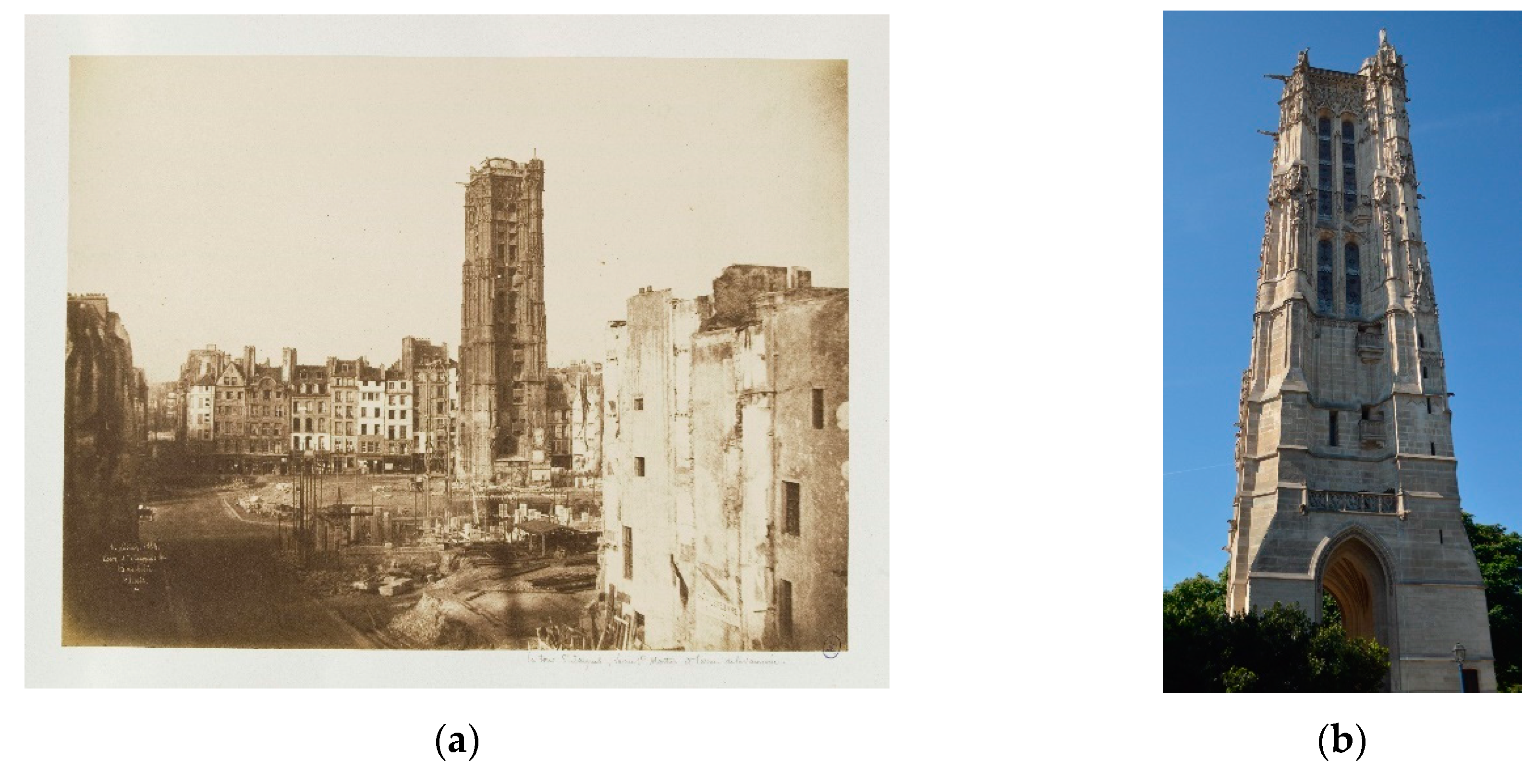
The first case study chosen is the Tour Saint Jacques (Figure 3) that is located in Rue Rivoli in Paris’s 4th arrondissement. This bell tower is in flamboyant gothic style and it has been inscribed in the UNESCO Heritage List since 1998 for its historical importance. The building, in fact, is the only evidence of the lost Saint-Jacques-de-la-Boucherie church, a Carolingian chapel destroyed in 1797 after civil unrest. The tower was saved from destruction because of its high architectonic value and after restoration, it was moved from its location and elevated on a decorative stone podium [27,28].

4.1.2. Les Halles

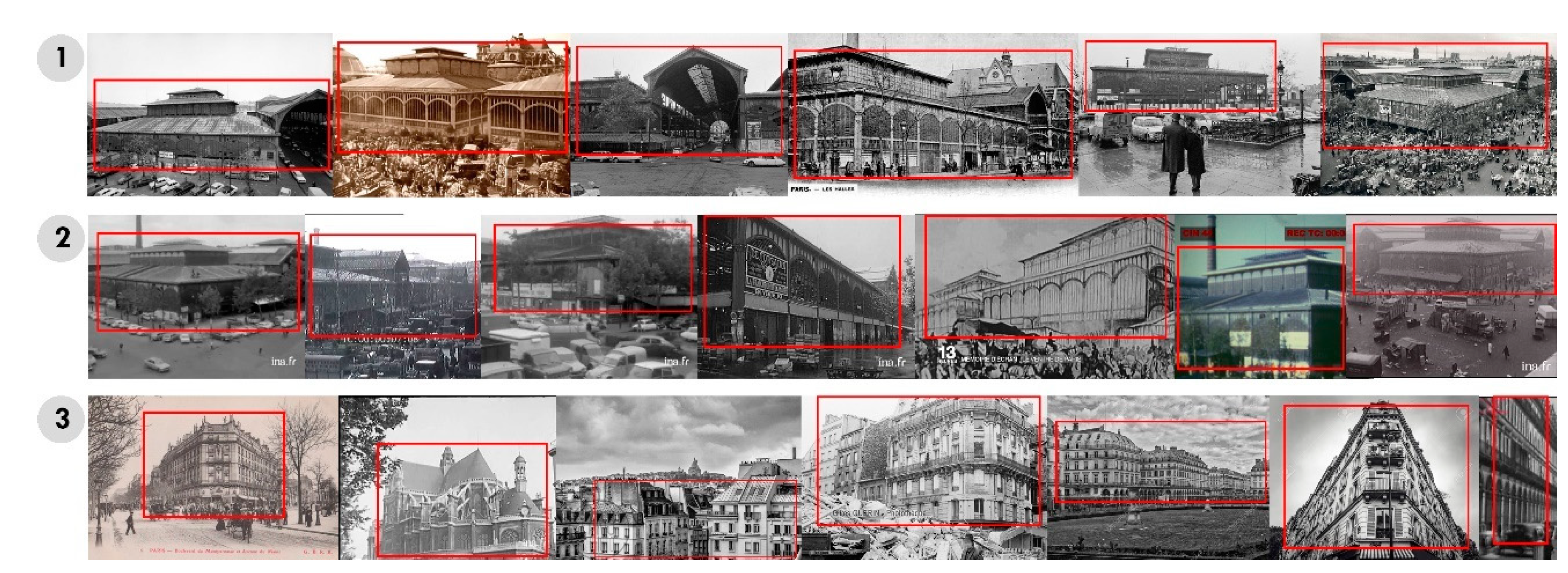
The pavilions of the ancient market of Les Halles (Figure 4) were built in Paris in 1852 by the architect Baltard. Les Halles constituted a nerve center in the city of Paris and became the object of numerous political and social debates [29,30]. Les Halles was destroyed in 1971 and now only two pavilions still exist: one is in Nogent-sur-Marne, Île-de-France, and one is in Yokohama, Japan.

One case study is of a place that still exists; the other no longer exists. This choice was made in order to represent two different aspects of architectural heritage. In fact, although the tower still exists, it is not in the original position, while Les Halles has been demolished, therefore they currently do not exist but were present until the 60s. However, both architectures appear in historical film footage from the 1910s until the 1970s. A lot of video materials, both documentary and fictional, which were set in the market and near the tower, were examined in several video archives in Paris (Lobster, Ina.fr CNC, Forum des Images, Gaumont Pathé Archives, Les Documents Cinematographique). Moreover, historical photographs, drawings and design projects were collected together with the films and a 3D model, obtained from a recent photogrammetric survey of the existing tower using UAV, made by Iconem in 2015. Therefore, they represent good case studies to test the proposed algorithm.

4.2. Dataset

Although much data was available on the tower and Les Halles, no suitable datasets existed. In order to implement the Neural Network, it was necessary to create new specific datasets.

The quality of primary data used in the implementation of the NN plays a crucial role in the achievement of good results. This strongly influences the training and a significant level of data entropy is necessary for the machine to learn the features of the object. It was easier to use the tower for this because, in addition to historical images retrieved for both case studies, it was also possible to collect hundreds of contemporary images with different backgrounds, lighting conditions and points of view. The methods used for the collection were the following: (1) web crawling; (2) ad hoc photographic survey in the new location of the tower; (3) historical archives consultation in Paris.

The experimentation was conducted in two different steps and on three different datasets, described in the following paragraphs.

4.2.1. Dataset 1: Reference Case—Tour Saint Jacques

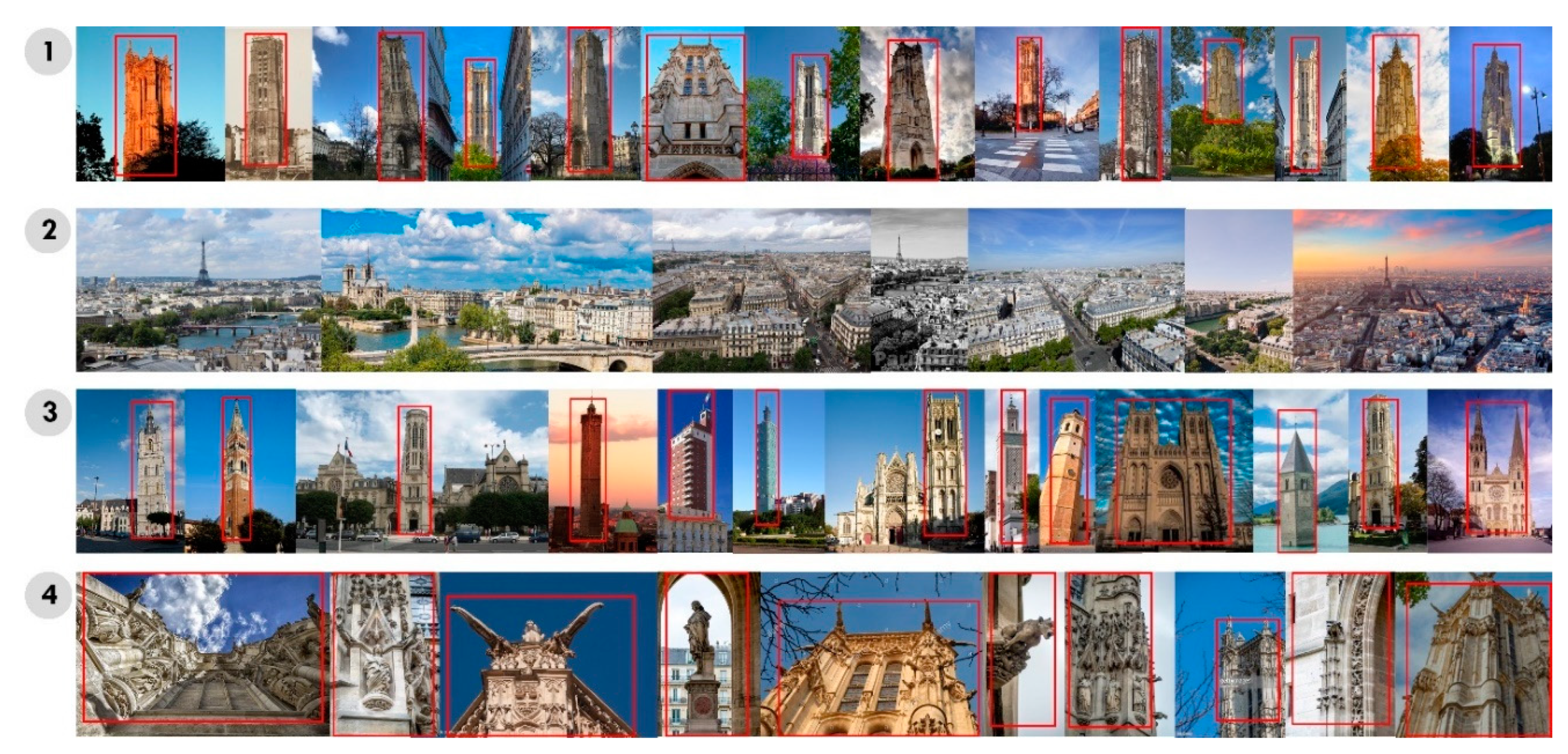
The first dataset was created with the aim to analyze two different Neural Networks on the best possible scenario of an existing heritage such as the Tour Saint Jacques case study. The collected images of the tower (Figure 5) were firstly divided into four categories based on the following criteria:

• Images of the entire tower both contemporary and historical;
• Views with the skyline of Paris because they appear in the film footage;
• Images that show monuments or architectures similar to the Saint Jacques tower for shape (for example other towers) or style (for example gothic architecture). These last images act as “negative matching” and can lower the incidence of the false-positive ratio in Machine Learning classification problems [31,32];
• Images representing only details or parts of the tower, since it is a typical situation when dealing with film footage that the camera moves shooting only parts of an object.

During the training phase different combinations in the number and type of images were extracted to improve the performance of the network, as shown in

Table 1. Description of the training and validation dataset 1 on the reference case of the Tour Saint Jacques.

Description	From Web	From Survey	From Historical Photographs	Number in Training			Number in Validation
				RUN A	RUN B	RUN C
Tour Saint Jacques	x	x	x	400	400	400	80
Landscape	x						80
Negative matching	x		x		200	200	80
Tour Saint Jacques Parts	x	x		80	80	80	80

and explained in the next section. Moreover, during validation, 80 images from each group of the dataset, named respectively as valid1, valid2, valid3 and valid4, were used to assess the quality of results from different perspectives (Table 1).

4.2.2. Dataset 2: Video

The second dataset was created to test the performance of the algorithm in a realistic case. For both case studies historical videos from archives in Paris have been collected. Despite the criticalities in retrieving these materials (see Section 2), a significant set of footage was collected, and their characteristics are described in

Table 2. Description of the video dataset of the Tour Saint Jacques.

Dataset	Duration	Year	Director	Type	Film	Colour	Archive
La tour Saint Jacques	9 min 47s	1967	J. Sanger	documentary		B&W	Ina.fr
Études sur Paris	76 min	1928	A. Sauvage	documentary	16 mm	B&W	CNC and VOD
Paris, Roman d’une Ville	49 min	1991	S. Neumann	documentary	16 mm	B&W	Forum des Images
Paris 2ème partie	4 min 44 s	1935	G. Auger	documentary	16 mm	B&W	Forum des Images
Passant par Paris	13 min 39 s	1955	P. Perrier	fiction	8 mm	B&W	Forum des Images
Vue Panoramique sur Paris	2 min	1954	A. Lartigue	documentary	16 mm	B&W	Forum des Images
Un film sur Paris	45 min	1926	C. Lambert, J. Levesque	documentary		B&W	Lobster
La nouvelle babylone	24 s	1929	L. Trauberg, G. Kozintsev	historical		B&W	Lobster
Paris, 1946	13 min	1946	J.C. Bernard	documentary		Colour	Lobster
La grande roue	4 min 20 s	1913		documentary		B&W	Lobster
Paris et ses monuments	7 s	1912	Pathe	documentary		B&W	Lobster

and

Table 3. Description of the video dataset of Les Halles.

Dataset	Duration	Year	Director	Type	Film	Colour	Archive
Crainquebille	1 min 32 s	1922	J. Feyder	drama	35 mm	B&W	Lobster
Les Halles 1960	35 min 15 s	1960		amateur		Colour	Lobster
Paris Mémoire d’écran	21 s			documentary		B&W	Gaumont Pathé Archives
Le ventre de Paris	5 min 55 s			documentary		B&W	Ina.fr
Le ventre de paris	3 min 11 s	2008	JP. Beaurenaut	documentary		Colour	Ina.fr
Les halles centrales	12 min 29 s	1969	J. Sanger	documentary		B&W	Ina.fr
La Destruction des Halles de Paris	3 min 28 s	1971	H. Corbin, J. Humbert	documentary	35 mm	B&W	Les Documents Cinemato-graphiques
Le dernier marché aux Halles de Paris	2 min 28 s	1969	G. Chouchan	documentary		B&W	Ina.fr
Les Halles: histoire d’un marché incontournable à Paris	2 min 5 s			documentary		B&W	Ina.fr
Les Halles de Paris en 1971	1 min 2 s	1971		documentary		B&W	Ina.fr
Les Halles	2 min 37 s			documentary		B&W	Ina.fr

.

4.2.3. Dataset 3: Real Case—Tour Saint Jacques and Les Halles

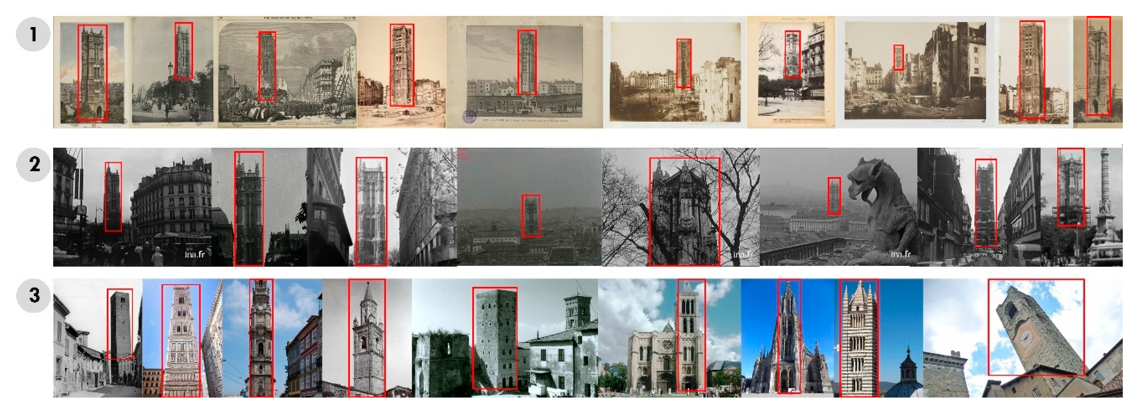
Evaluating the implementation of the NN on film footage in which a lost monument appears means that it is not possible to use a dataset that contains contemporary images of the building since it no longer exists. For this reason, the third dataset (Figure 6 and Figure 7) was created to test the algorithm to this real case on both case studies. With this aim, the categories of images were categorized in three different groups:

• Historical photographs of the monument.
• Historical images, both photographs and frames extracted from the video dataset in which the searched monument appears.
• Negative matching, for the tower this coincides with the third group of the first dataset; for Les Halles are the images with buildings of Paris that appear in the film footage.

Moreover, for the tower some images were collected in a new validation group called valid5 and added to the previous dataset 1 to test the algorithm on this reference case. For Les Halles the validation group on which the algorithm was tested is called valid1. The number of images used during the training and the validation and the combinations for the different runs are shown in

Table 4. Description of the training and validation dataset 3 on the real case of the Tour Saint Jacques.

Dataset	Number in Training RUN												Number in Validation
	T1A	T1B	T1C	T1D	T1E	T1F	T2A	T2B	T2C	T2D	T2E	T2F	VALID5
1. Tour Saint Jacques—Historical Photographs	50	42	35	25	15	5	25	20	10	5	7	2	0
2. Tour Saint Jacques—Frame	0	0	0	0	0	0	25	22	25	20	8	3	29
3. Negative matching	50	42	35	25	15	5	50	42	35	25	15	5	0

and

Table 5. Description of the training and validation dataset 3 on the real case of Les Halles.

Dataset	Number in Training RUN												Number in Validation
	T1A	T1B	T1C	T1D	T1E	T1F	T2A	T2B	T2C	T2D	T2E	T2F	VALID1
1. Halles Historical Photographs	50	42	35	25	15	5	25	17	23	16	6	0	32
2. Halles Frame	0	0	0	0	0	0	25	25	12	9	9	5	46
3. Negative matching	50	42	35	25	15	5	50	42	35	25	15	5	0

and will be further explained in the next section.

5. Results and Discussion

In this section, the Neural Network results are discussed. In the first subsection, the training stage is detailed and the network model choice is discussed alongside the type of training dataset and the probability threshold selection. In the second subsection, the influence of the training dataset size and source is discussed. In the third subsection, the network is evaluated in a realistic scenario underlining the behaviors of the metrics more closely related to the end-user activity. In the fourth subsection, a brief discussion of the computational power required to utilize neural networks is presented. Finally, in the fifth subsection, the Neural Network results are discussed with respect to the final step of the pipeline, i.e., the photogrammetric reconstruction.

5.1. Network Model Selection and Tuning

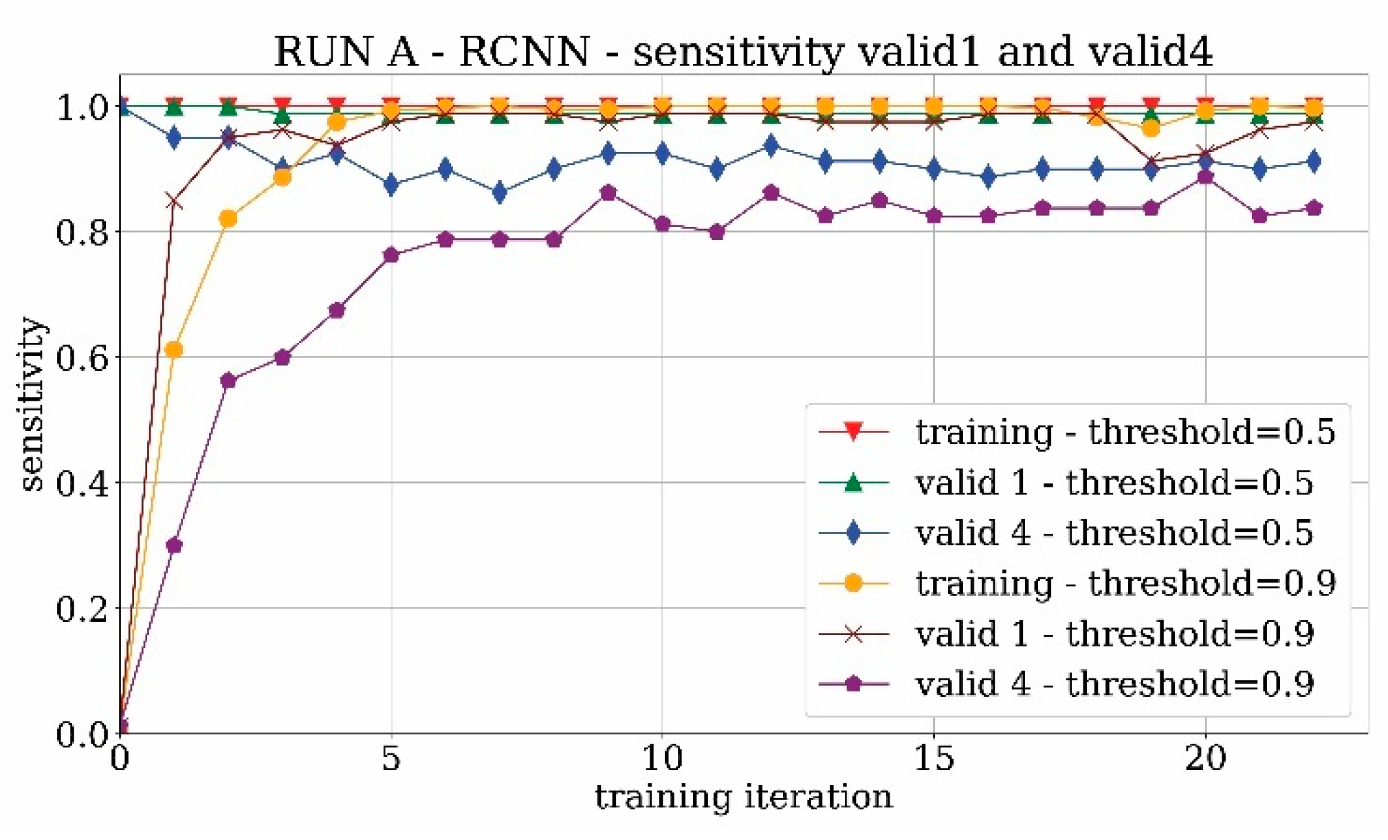
The first part of training experimentations is based on the Tour Saint-Jacques case due to the high availability of past and modern pictures in addition to some sets of historical videos. The experimentation started with the adoption of the RCNN network, also called “accurate network” in the Luminoth reference. In the first training—labelled as RUN A—only positive matches, represented by images of St. Jacques tower with complete or partial views (datasets 1 and 4) were used. 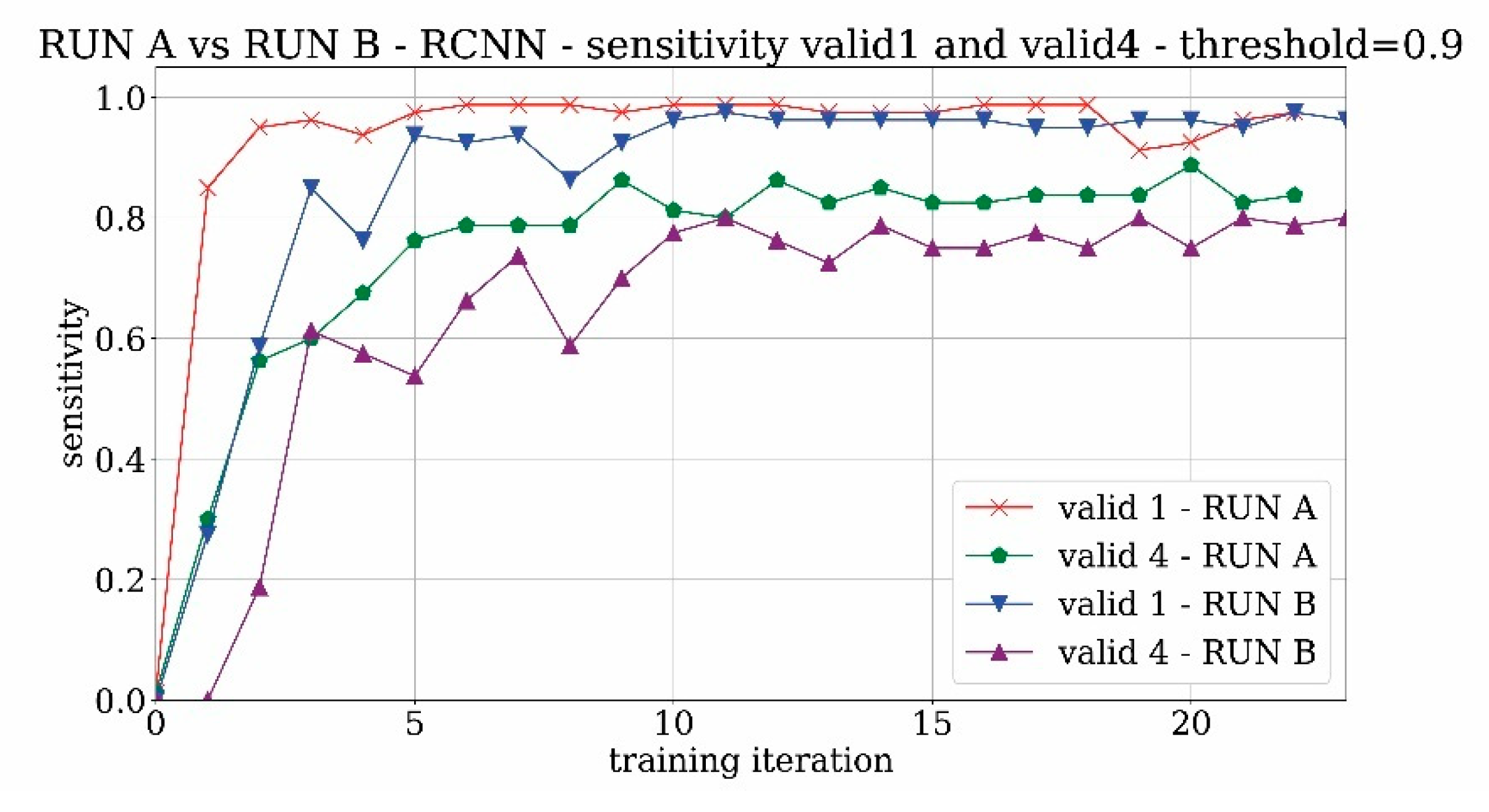The results of the sensitivity analysis conducted on the training and validation sets containing the tower (respectively valid1 and valid4) are shown in Figure 8 considering two reference probability acceptance thresholds equal to 0.5 and 0.9, respectively.

What can be clearly seen in the graph is that the network rapidly converges and reaches a very high value of training accuracy (i.e., sensitivity), as well as very high values of validation accuracy for the valid1 set which includes only images of the entire tower. The accuracy is more limited (around 0.8) for valid4 because partial views of the tower are not always detected. Furthermore, as expected, the network becomes more selective by increasing the probability threshold, and the sensitivity tends to significantly decrease, especially for valid4.

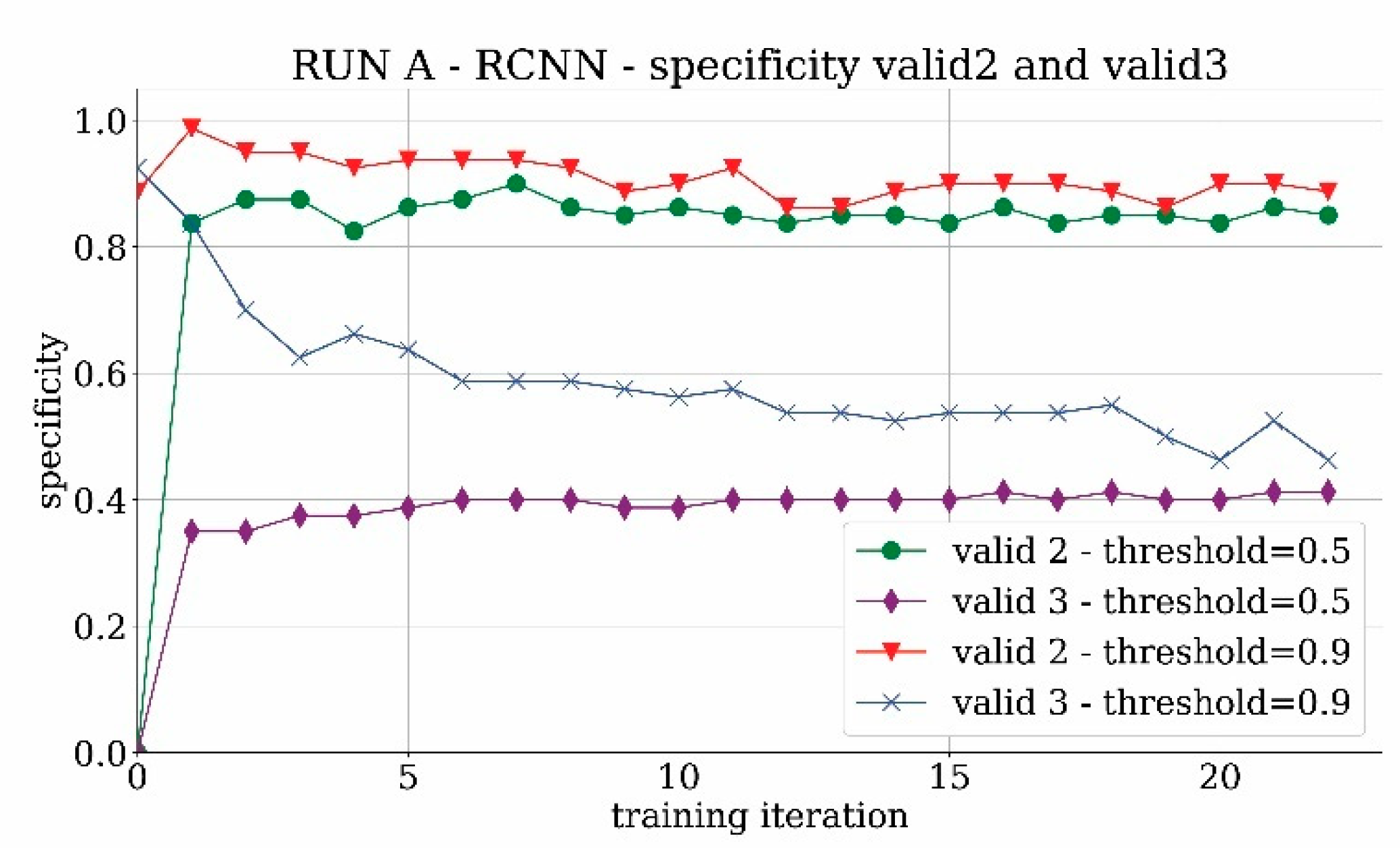
The validation behavior of the validation sets that contain the images without the tower is shown in Figure 9 for both valid2 and valid3 sets. For the valid2 dataset which contains images with the landscape around the location of the tower, the trend is quite good and reaches a specificity value of 90%. For the valid3 set, the presence of non-Saint-Jacques towers creates confusion in the network learning and leads to poor results close to 50% of specificity. It means that the network is not able to distinguish the real tower from other similar towers with high accuracy. By increasing the threshold, the network becomes more selective and the problem of false positives is therefore at least partially alleviated.

The difference between the specificity results of valid2 and valid3 sets is not surprising. Since the training runs start from pre-trained networks, it is expected that common categories are already stored—in the neural network sense—in the initial weights of the network. Indeed, from the validation results represented in Figure 9, it can be ascertained that only a few false positives correspond to landscapes whereas a significant amount of shapes similar to the tower are misinterpreted by the network as the Tour-Saint Jacques tower. In this scenario, to address the most frequent false positive type, the valid3 image set, containing shapes similar to the searched Tour Saint Jacques, was used as a negative matching set in the subsequent runs.

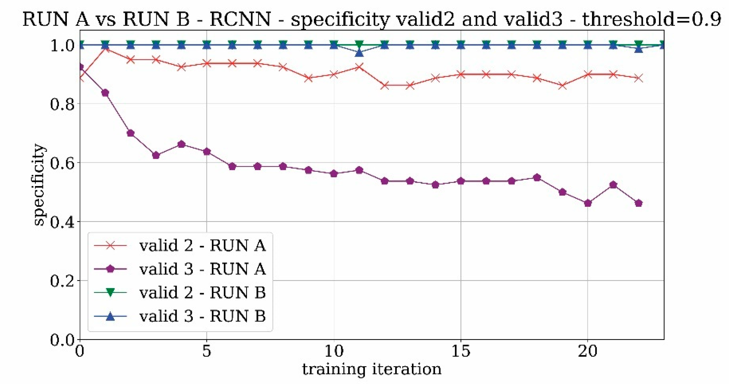
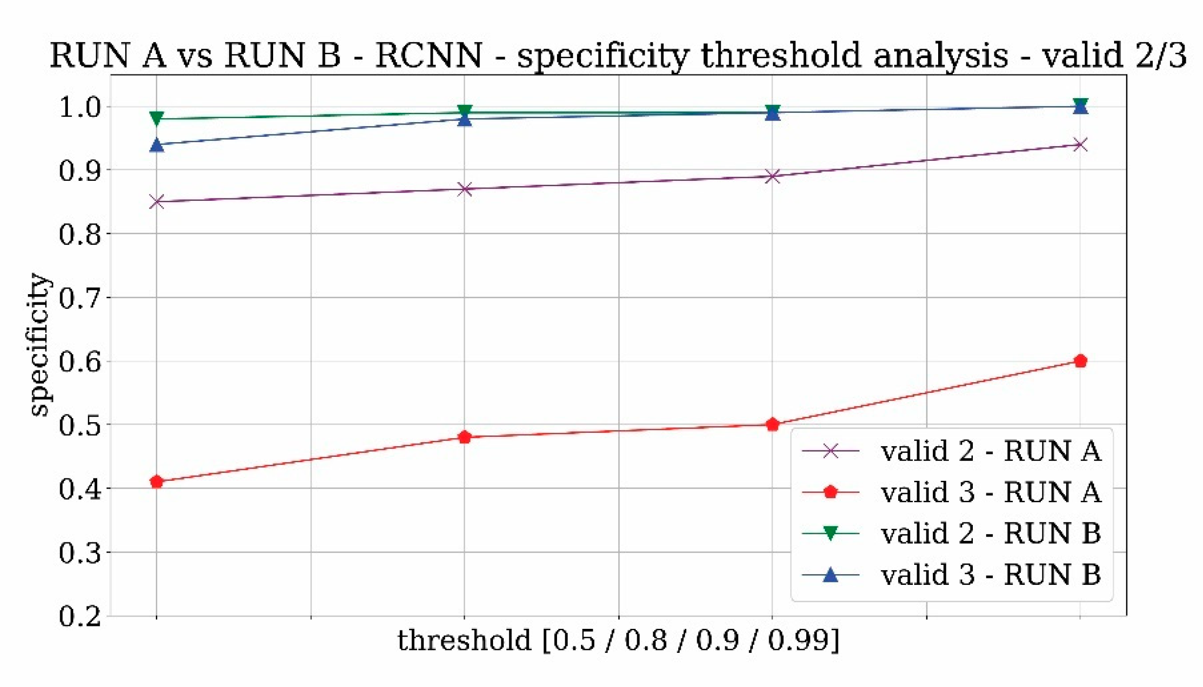
The second training RUN B was still based on the Faster-RCNN network but it was performed including the negative matching set of images with the aim of improving the performance of the network minimizing the false positive results. In Figure 10 the sensitivity analysis of the RUN B network is shown. As expected, in comparison with the previous training scenario, the network becomes more selective. The graphs reveal a slight degradation of the recognition of the true positives compared to RUN A where negative matching images are not used in training. However, in terms of specificity—as shown in Figure 11—the problem of false-positive results seems to be mostly solved. The significant specificity improvement of RUN B compared to RUN A demonstrates that using valid3 as the “negative matching” set was an effective choice. Overall, the advantages of RUN B training outweigh the disadvantages. However, according to the use of the algorithm, it could be decided to always prefer sensitivity, so RUN A would be slightly better.

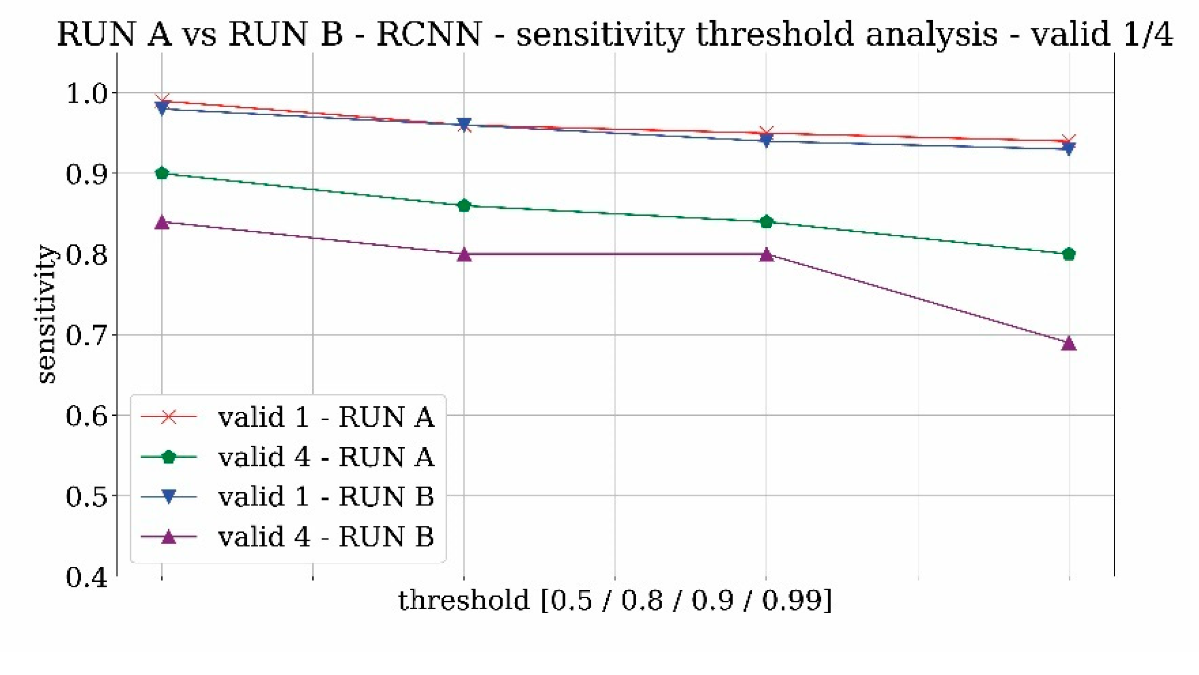
Figure 12 and Figure 13 reveal the analysis of sensitivity and specificity trends for the two trainings RUN A and RUN B in order to evaluate the influence of the probability threshold on the results. The value of sensitivity is likely to decrease with the threshold whereas the specificity is expected to increase. From both figures, it results that 0.9 can be a good compromise on the threshold selection.

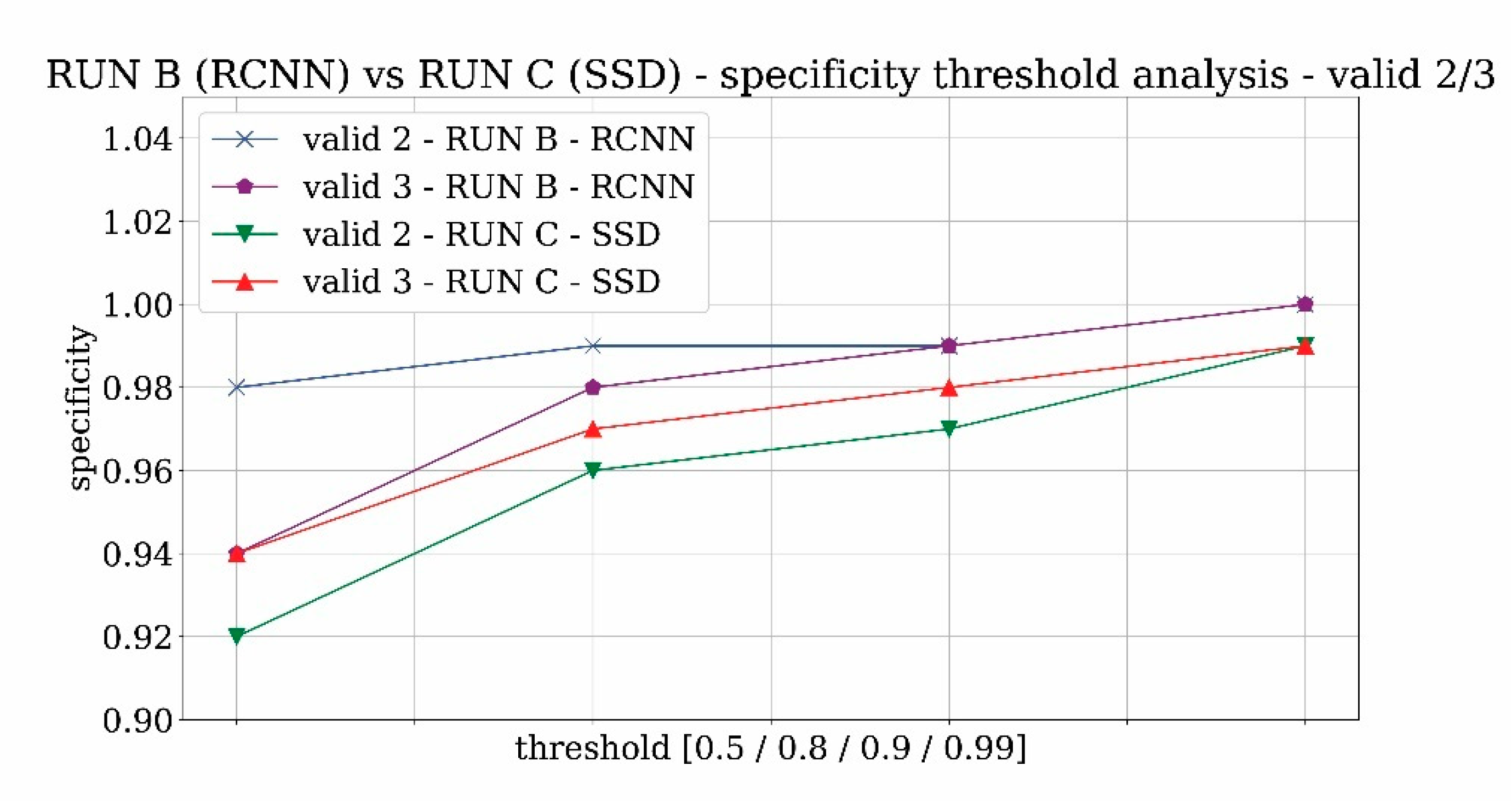
The third training RUN C which was attempted is based on the SSD network, while keeping fixed the training dataset (including negative matches). The results of the comparison between the RCNN network and the SSD network are shown in Figure 14 and Figure 15. What can be seen is that in positive cases the SSD network provides better values of sensitivity at least for the valid 4 set (Figure 13). However, from a visual inspection, it turns out that the images which are detected only by the SSD network are usually very poor-quality images or even drawings and therefore not suitable for the photogrammetric extraction. In terms of specificity, from Figure 15 it turns out that the values for both networks are high. Especially for the RUN B the values are very close to the ideal value of the unit. On the other hand, from Figure 15 it results that there is a specificity degradation for the SSD network. Even though, the specificity degradation seems small—around 2%—it is worth noting that in realistic scenarios the amount of negative images is huge and having 2% of false positives may be incredibly costly for the end-user activity.

Summarizing, the SSD network is lighter in terms of computation than the Faster-RCNN and can detect more (usually poor quality) true positives, but at the same time it detects a too high number of false positives. The consequence is a greater number of videos to watch for the user. For these reasons, the threshold value of 0.9 together with the Faster-CNN were identified as the most reliable feature of the network to use in the next experimentations.

5.2. Assessment of the Training Dataset

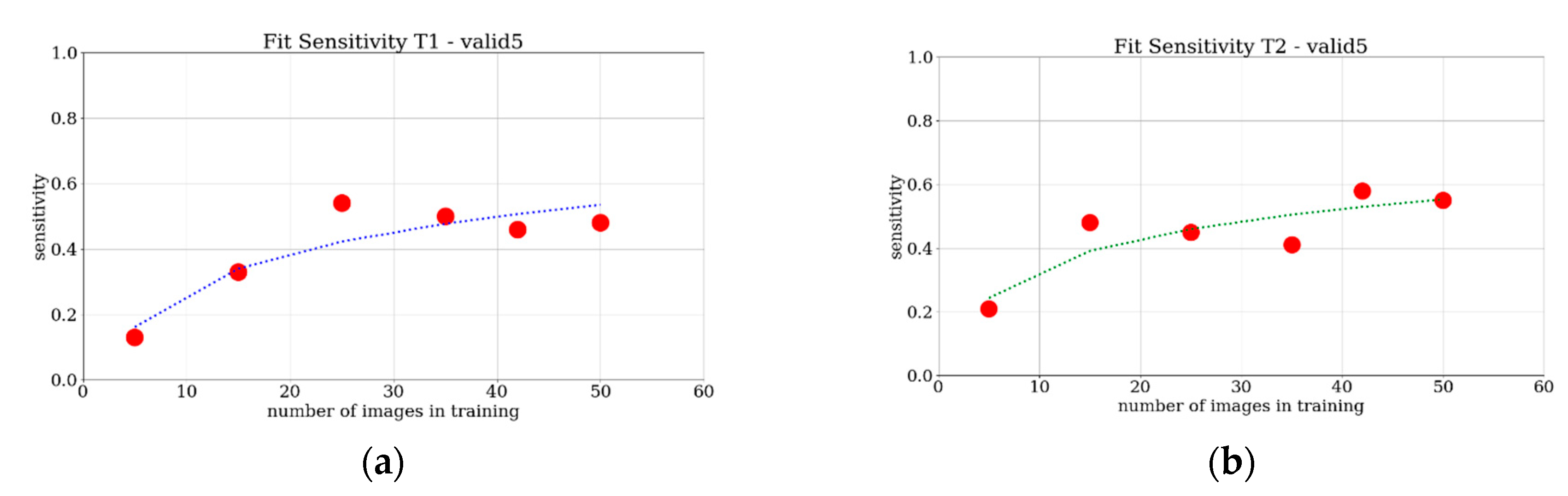
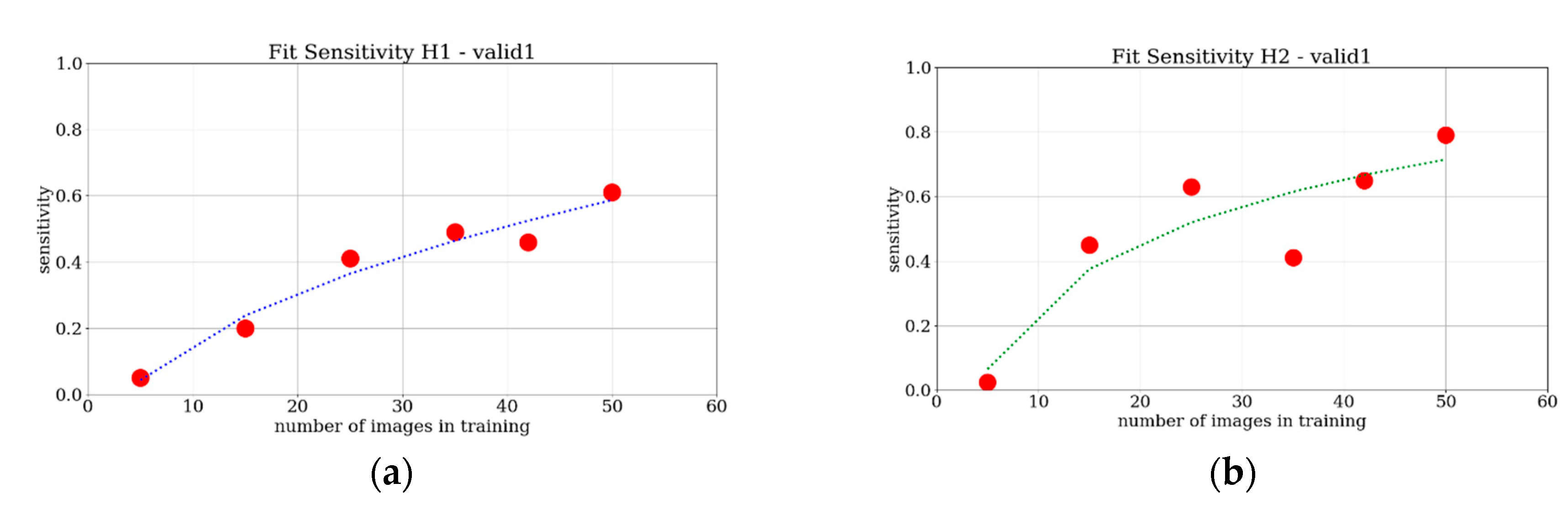
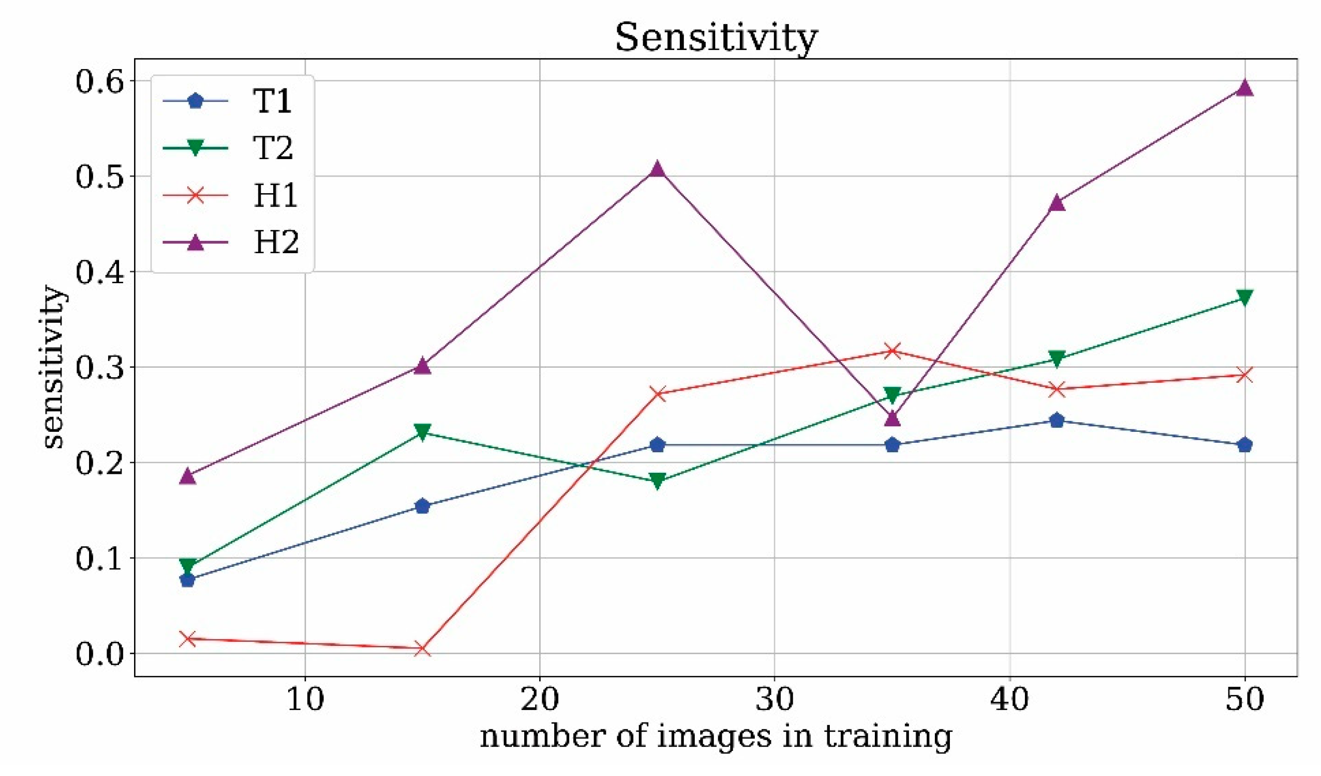
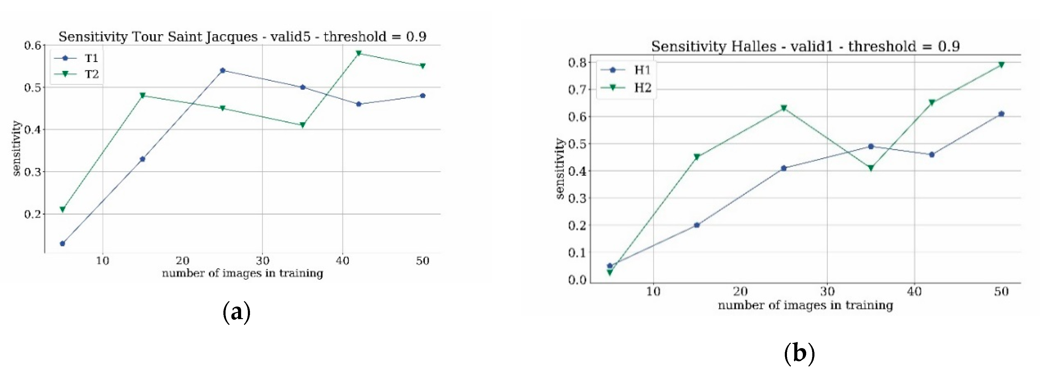
The previous investigation identified Faster-CNN as a suitable model of the network to utilize. It also highlighted the advantage of inserting negative matching in the training datasets. Finally, the selection of 0.9 as the object detection threshold proved to be a good compromise. The following part of this paper moves on to examine the application of these assumptions to a real case. When architectural heritage is lost, only historical archival material is available. For this reason, in the following analyses only historical images, both photographs and frames from videos, were used in the training phase. Considering the difficulty of finding the first monument images needed for training, considerations need to be given to both the source of suitable images of the monument and the number of images required for a good quality training phase. In order to investigate these issues in this study, several training phases were performed. First, two different kinds of runs were chosen. In the first one, the training was performed using only historical photographs, in the second one also the frames extracted from historical videos were added to the dataset. To enhance generality, both the case studies of the tower and of the pavilions were tested: the terms T1 and H1 refer to the runs with the training datasets that contain only historical photographs, respectively, for the tour Saint Jacques and Les Halles. The terms T2 and H2 refer to the runs that also employ the frames extracted from videos. Furthermore, with the aim of calculating the minimum number of images required to achieve acceptable training results of the network, six different runs were processed with a decreasing number of elements in the dataset: these runs are labeled as A-B-C-D-E-F. For example, T1A stands for the run trained using 50 true images and 50 negative matchings, considering only historical photographs. On the other hand, T2A stands for the run trained using 50 true images and 50 negative matchings, considering 25 historical photographs and 25 video frames containing the monument. The other letters are related to the number of training images as follows: B = 42, C = 35, D = 25, E = 15, F = 5. A comparison among each case study was performed by validating the network against datasets that contained only historical images, called valid5 (valid1) for the tower (Les Halles) test cases. The evaluation was achieved considering single frames of the videos.

The results are provided in Figure 16, Figure 17 and Figure 18, where the sensitivity is plotted against the number of training images for each test case and each source of training images (only historical photo or combination of historical photo and video frames). Since the involved test datasets always contain the searched monument, the sensitivity equals the accuracy.

The provided results show a monotonically increasing trend of the sensitivity when the number of images increases, for all of the four considered evaluations. Furthermore, a saturation trend for all of the cases can be ascertained. To achieve reasonably saturated results, around 25 images were required for the tower case, whereas 35 images were needed for the Les Halles case. What is interesting in these charts is that there is no great difference between the trend of the four curves, when compared to the curve fittings based on the simple power-law f(x) = a + b∙x^c. This is represented in Figure 16 and Figure 17. Even though this analysis is limited to two test cases, a first brief indication is that with a minimum of 30 images it is possible to train the network adequately to find the requested object. For low numbers of images, in particular the T2 and H2 cases present a measurable advantage in terms of sensitivity performances compared to the T1 and H1 counterparts. For a higher number of training images, the advantage is smaller and more difficult to detect. All in all, at least for these two test cases, the source and the type of the images do not significantly influence the performance of the learning process of the network. Instead, the number of training images is crucial to achieving good quality training.

5.3. Network Evaluation in a Realistic Scenario

5.3.1. Frame-Based Metrics

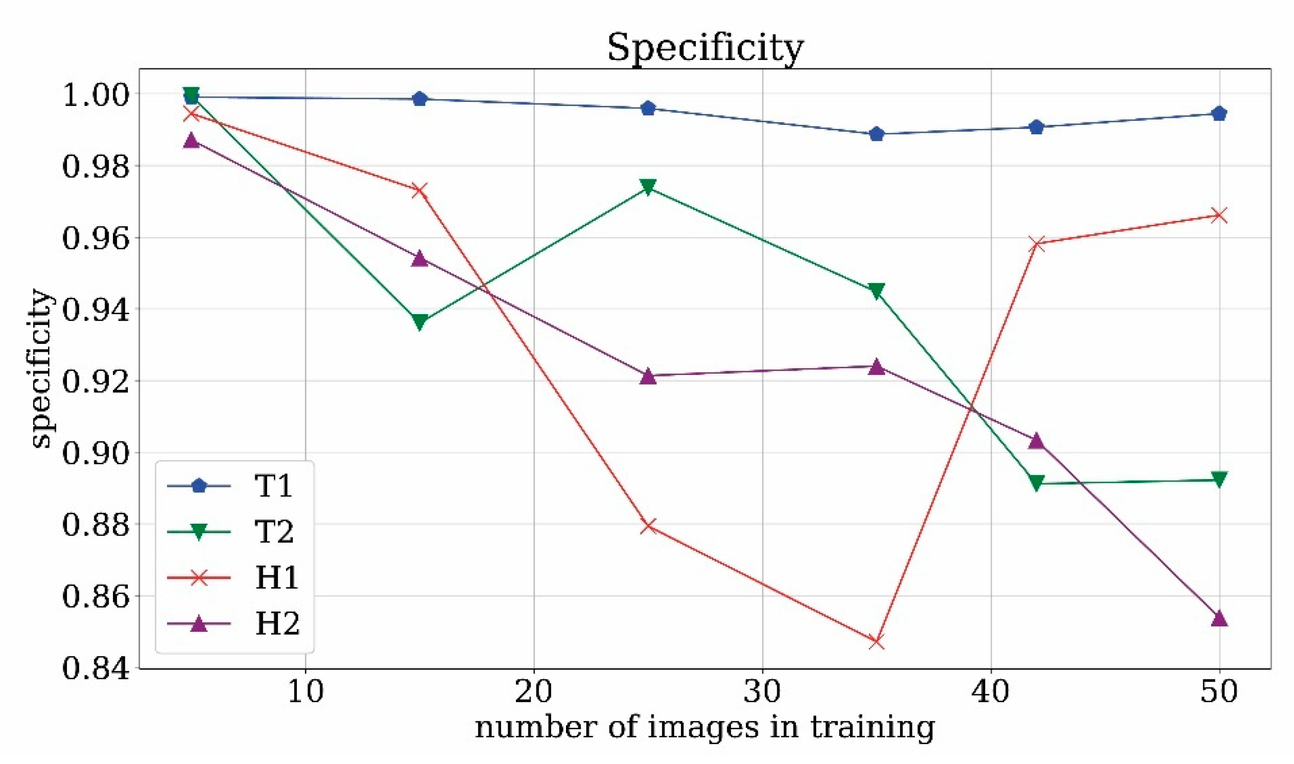
In the previous section, a detailed investigation of sensitivity performances when varying the number and source of training images was provided. The sensitivity basically summarizes the capability of the network to detect the searched monument but does not provide information about the time save achievable using Neural Networks in comparison to manual procedures. In order to discuss the latter point, the first quantity to be evaluated is the specificity. In order to evaluate meaningful specificity values, a realistic test dataset is recommended. Indeed, in a realistic scenario where the amount of positive and negative is as balanced as expected in a real archive, it is possible to evaluate the best compromise between the metrics to be maximized. For this reason, the same analysis varying the number of training images is repeated considering the videos as the test dataset (as usual, the video frames used during the training are not used in the test dataset). Starting with the use of the standard metrics applied to video frames, the resulting charts are provided in Figure 19 and Figure 20 for both sensitivity and specificity parameters. As regards the sensitivity, the trends against the number of training images are similar to the previous sensitivity analyses, but the absolute values are slightly smaller, as expected considering that the average quality of video frames is lower than the historical photos used in the previous test datasets. All in all, the analysis shows that the monuments correctly detected as positive are less than half of the total positive ones, therefore some information is lost. As regards the specificity, the trends are not monotonous; the ability to recognize true negatives fluctuates but does not show a definite trend in all four cases. The specificity values are always greater than 84%. This percentage is related to the time-saving advantage for the end-user, but a direct interpretation of the value in this sense is not obvious. Moreover, it is worth noting that the specificity value is limited by the fact that the test videos were manually selected to contain at least one occurrence of the searched object, such a circumstance does not correspond to a realistic archive analysis.

5.3.2. Time Interval-Based Metrics

As discussed in Section 3, the evaluation of metrics based on time-intervals may be more suitable to realistically analyze the quality of trained networks concerning the end-user activity.

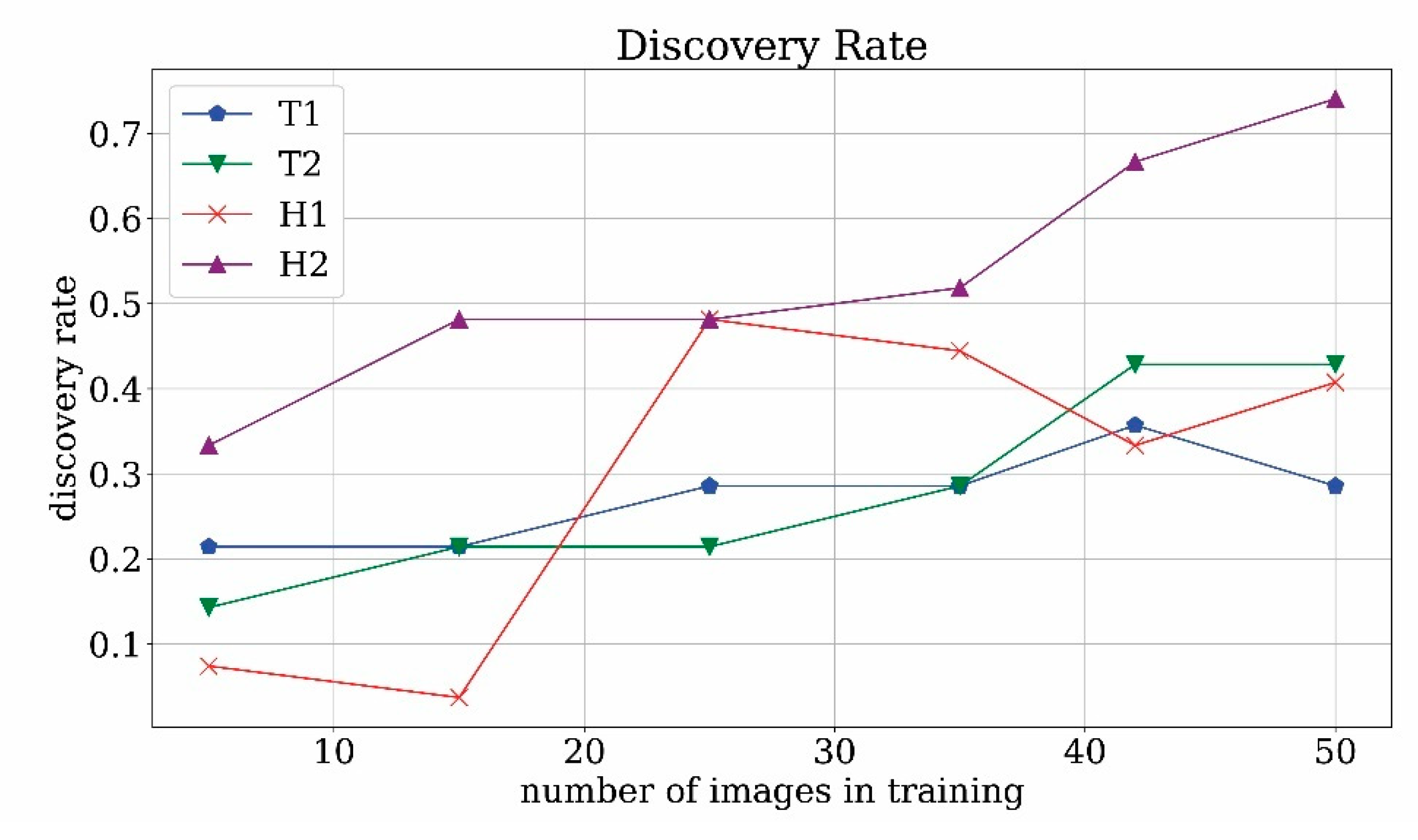
In Figure 21 the time interval discovery-rate is plotted against the number of training images for T1, H1, T2, H2 cases. The percentage of correctly predicted intervals in which the monument appears found by the runs T2 and H2 of the network, in which both historical photographs and frames were used, reached a higher number than the T1 and H1 since the value of probability to detect the correct object is around 75% against 50%. As previously explained, the evaluation of the discovery rate is somehow related to the frame-by-frame sensitivity, even if calculated on intervals. Comparing the results of discovery-rate and standard sensitivity, it is evident that using a metric based on time intervals leads to an evaluation less strict than the counterpart based on the frame, but the time interval perspective is more significant from the point of view of the final user.

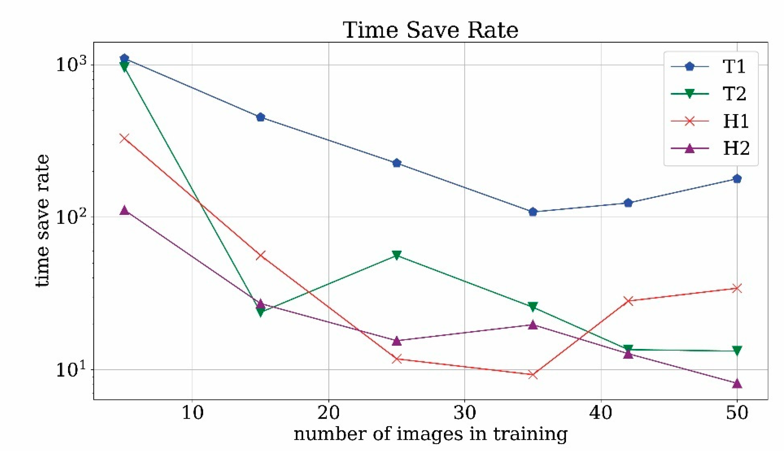
In Figure 22, the time save parameter is plotted against the number of training images. It turns out that for T2 and H2 runs with a low number of images the time save is around 1000. However, in this range the discovery rate is very poor. With the increase in the number of images the value decreases around 10/50 which is still a satisfactory value for the time save. It is expected that the value increases, even more, when generic video archives are taken into consideration.

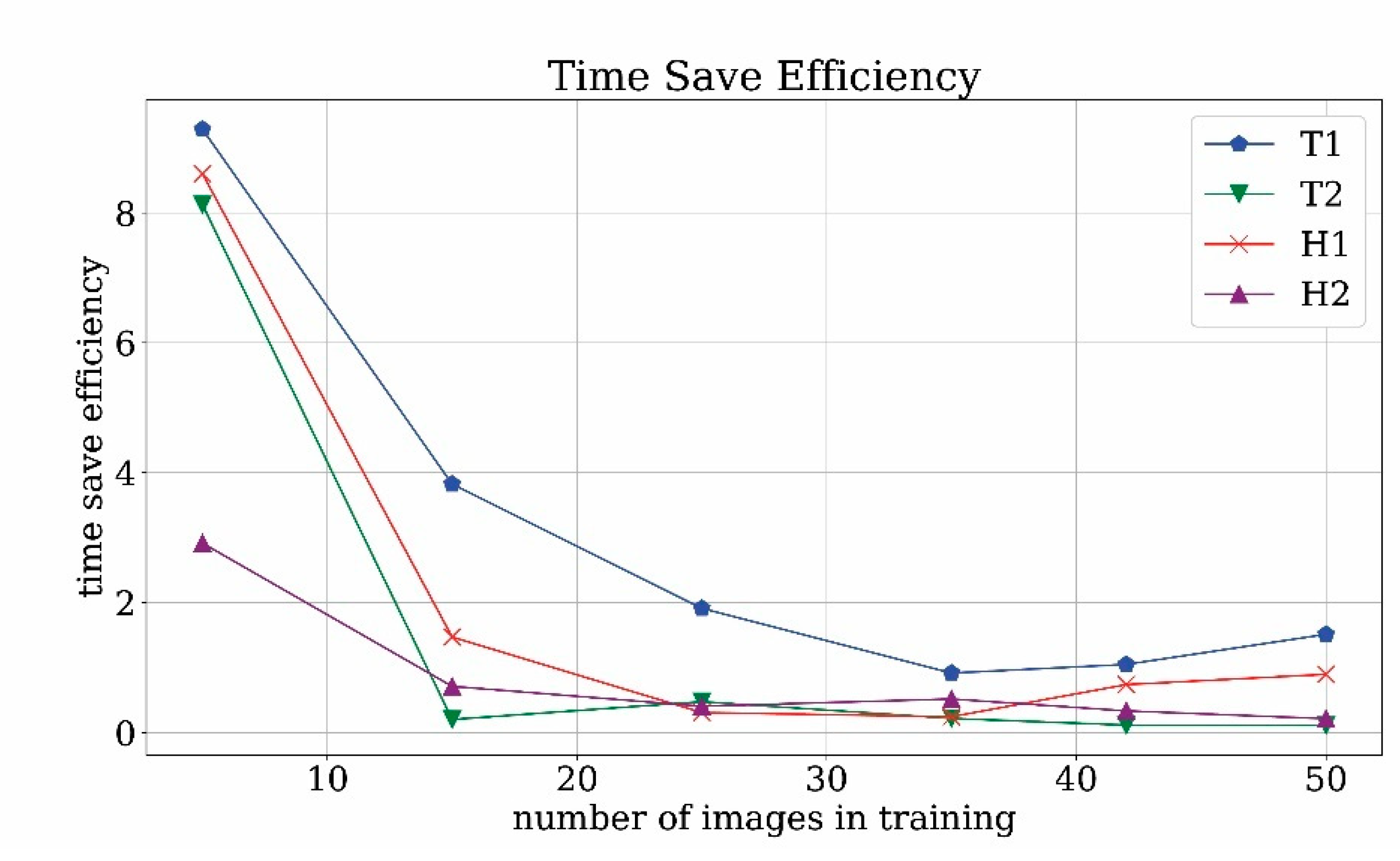
In order to get rid of the dependency on the type of considered videos, it is possible to compare the time save rate with the ideal time save rate, thus defining the time-saving efficiency. Time save efficiency results are plotted in Figure 23. For a low number of training images, the time save efficiency is higher than unity and this is due to poorly trained network, which is not capable of detecting both true and false positives. For mid-range and high-range numbers of training images, the efficiency is order 1 which means that the operator time save is close to the ideal time save. Obviously, this is possible because not all of the objects are correctly found. However, the found images are usually the best quality ones and therefore are more usable for the next steps of our pipeline. In this scenario, the time save rate efficiency close to unity can be considered an optimal result.

5.4. Hardware Analysis: High-Performance Computing vs. General Purpose

The use of GPUs (Graphical Processing Units) has emerged as a cutting-edge technology in the context of Machine Learning due to the high computing power achievable and the relatively low amount of energy consumption. Modern frameworks for neural networks support GPU computing. GPUs are available in common home computers or small work-stations, but GPUs are nowadays also protagonists as accelerators of High-Performance Computing (HPC) clusters. In

Table 6. Hardware comparison.

NVIDIA 630M	NVIDIA K40	NVIDIA P100	NVIDIA V100	NVIDIA 1650
2012	2014	2016	2018	2019
Low-range Laptop	HPC	HPC	HPC	Mid-range Laptop
30 s/image	1 s/image	0.5 s/image	0.3 s/image	9 s/image

, we report the time required to process an image during the training stage.

To follow the evolution trend of the GPUs, results based on low/mid-range GPUs were reported up to results from top GPUs used in HPC centers. The order follows the release date of the devices. The type of GPU is also described as distinguishing HPC GPUs from consumer GPUs. It turns out that the improvement over the years is important, with a speed-up around 3 years after 5 years. Another very important point is the advantage of using HPC-oriented GPUs compared to normal laptop GPUs. The difference in timing is very marked. For complete training, the elapsed time may pass from several tens of days to less than 24h. In the massive inference phase, the use of HPC platforms can become a fundamental requirement.

5.5. Photogrammetry: Processing and Evaluation

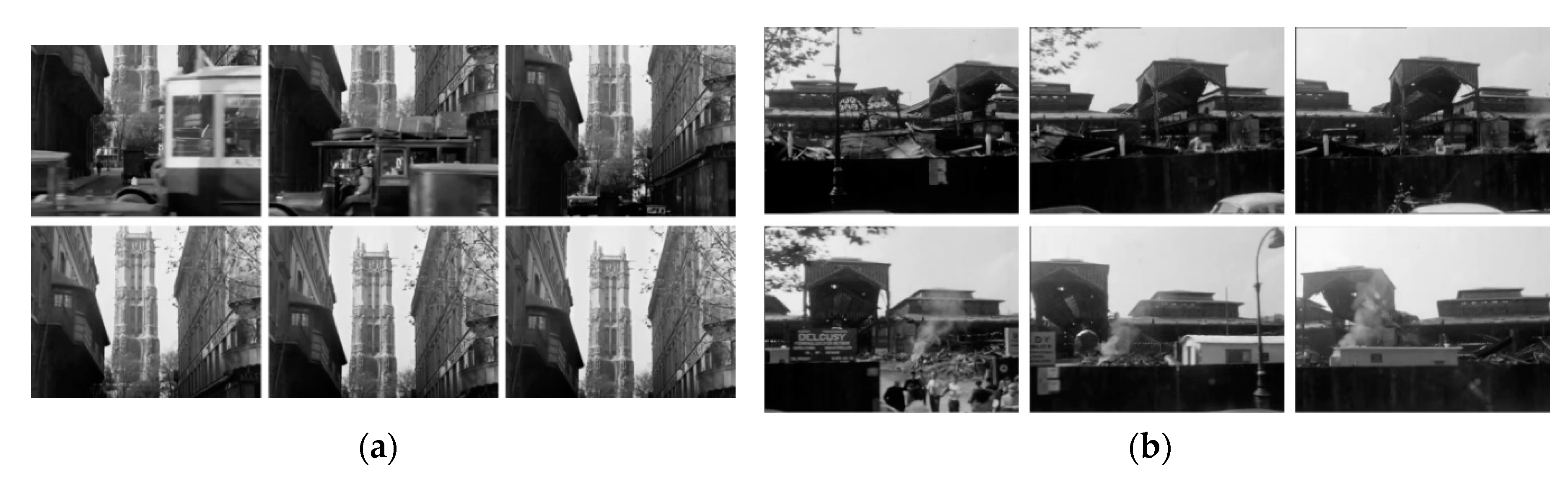
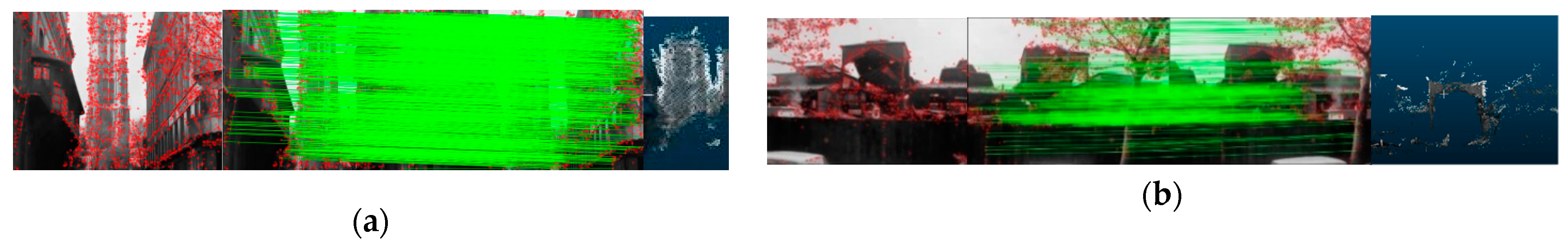
The frames that contained the architectural heritage detected were automatically extracted from the film footage and used during the photogrammetric process. Two different films to be processed were chosen among the footage correctly detected by the Neural Network. The first one is “Études sur Paris” from the CNC-VOD archive (Figure 24a) and contains sequences of images of the Tour Saint Jacques, taken with tilting camera motion. The second video, with images of pavilions, is “La Destruction des Halles de Paris” found in Les Documents Cinematographiques archive (Figure 24b). The type of camera motion in which the video was shot is the trucking. The two films present the characteristics shown in

Table 7. Technical features of the films used during the photogrammetric processing.

Film	Gauge	Focal Length	Digital Format Resolution	N° Frame	Camera Motion
Études sur Paris	16 mm	25 mm	480 × 360 pixels	16	Tilting
La Destruction des Halles de Paris	35 mm	35 mm	492 × 360 pixels	49	Trucking

:

Figure 25 shows the results of the SfM pipeline applied to the two case studies.

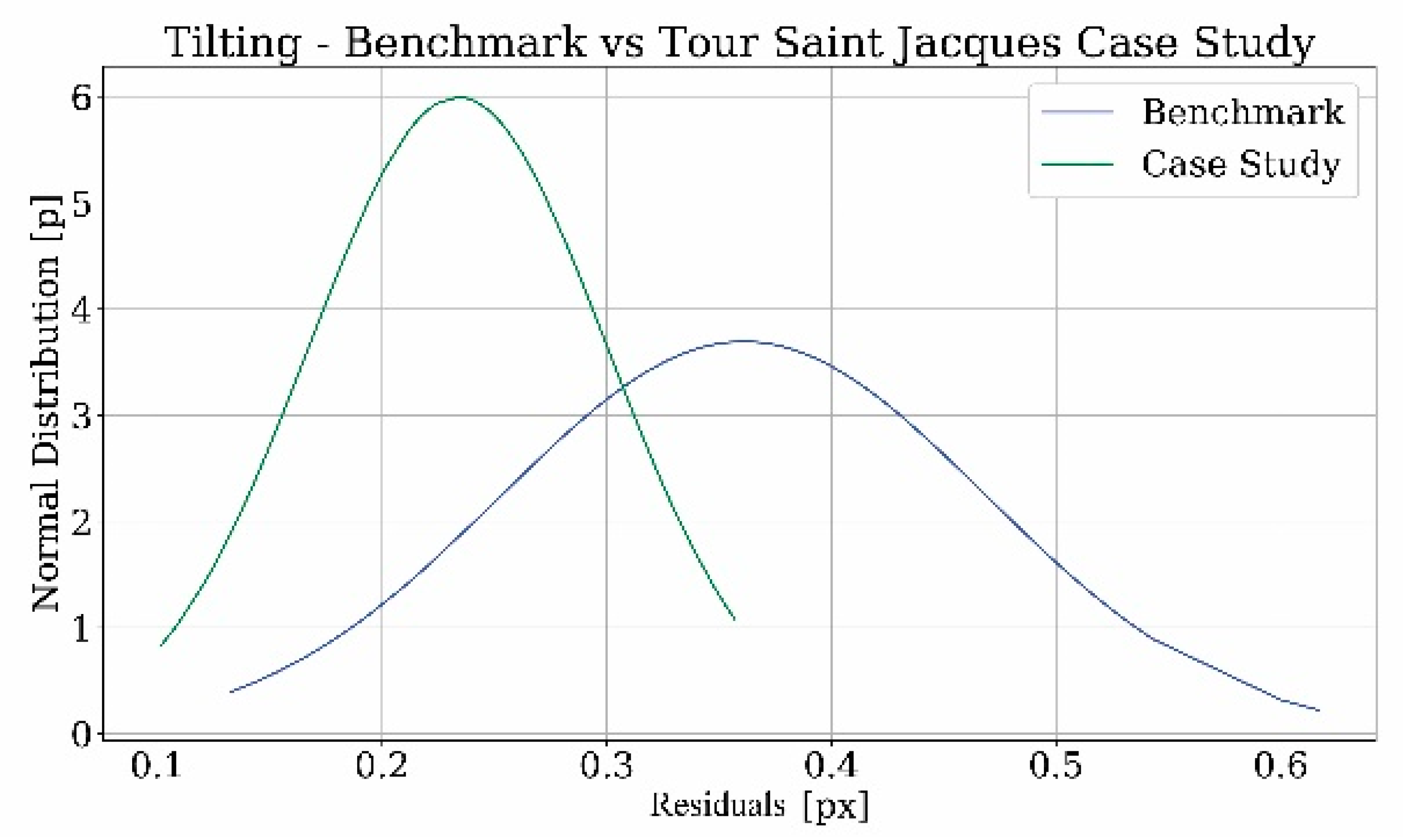
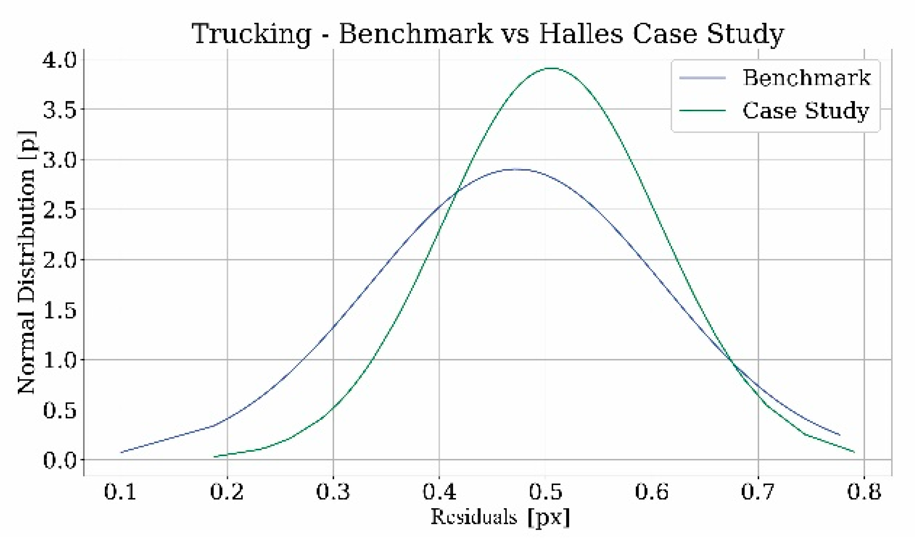
In order to assess the quality of the point clouds obtained from the photogrammetric process, the values of the residuals were used for the calculation of the mean and standard deviation. The following graphs analyze the trend of the data and the comparison with the benchmark (Figure 26 and Figure 27).

In addition, the minimum and maximum values were converted to centimeters with the calculation of the Ground Sample Distance (GSD). The results are reported in

Table 8. Mean, standard deviation, Min and Max values of residuals.

TOUR SAINT JACQUES
Case	Mean		St Dev		Min Residual		Max Residual
	px	cm	px	cm	px	cm	px	cm
Benchmark	0.36	0.10	0.10	0.80	0.13	0.10	0.60	0.80
Case study	0.23	0.33	0.06	0.08	0.10	0.14	0.35	0.50

; for the tower a distance of 15 m was considered (GSD benchmark = 1.2 [cm/px], GSD tower = 1.43), and in

Table 9. Mean, standard deviation, Min and Max values of residuals.

LES HALLES
Case	Mean		St Dev		Min Residual		Max Residual
	px	cm	px	cm	px	cm	px	cm
Benchmark	0.47	5.20	0.13	1.40	0.10	1.10	0.77	8.70
Case study	0.50	11.80	0.10	2.30	0.18	4.20	0.79	18.60

for the pavilions, a distance of 120 m was considered (GSD benchmark = 11.2 [cm/px], GSD Les Halles = 23.6 [cm/px]).

The graphs show that the curves in both the case studies follow the Gaussian distribution as in the case of the benchmark. What it is noted from the tables is that when comparing the two results, the differences between the values of the case study related to the tower and the benchmark are not significant. Instead, concerning Les Halles, the values in pixels are almost the same, but, after the transformation in centimeters through the GSD calculation, the values of the case study are higher than those of the benchmark. These disparities could derive from the approximation about the focal length of the camera used to shoot the film footage and the taking distance. For this reason, a margin of error has to be considered in this evaluation.

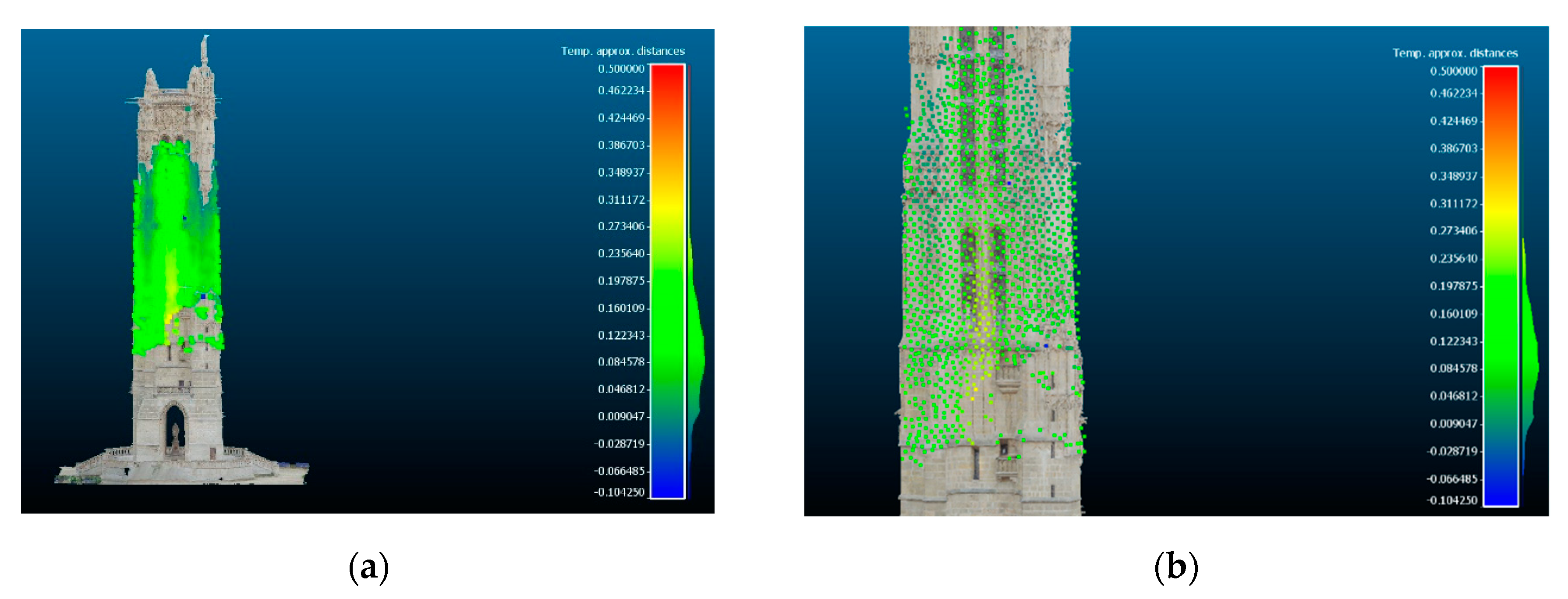
Finally, the point cloud of the tower obtained by the process, although of low density, was compared with the 3D model of Iconem. The comparison (Figure 28) showed that the calculated distances between the model mesh and the resulting point cloud were less than 0.5 pixels.

Despite some limitations derived from the lack of certain information about the technical features of the camera and the film used to shoot the videos and the unavailability of a precise 3D model for the case study of Les Halles, since it no longer exists, these findings are very encouraging for the metric certification of the models obtained. This represents a fundamental aspect of the scientific documentation of heritage sites.

6. Conclusions

This study sets out to recognize (in an automatic way) lost architectural heritage in film footage in order to create a 3D model that can be metrically certified. The experiment focused on the reduction of human effort in the detection of the searched object and increased efficiency in the work of the operator in the archive. In order to achieve this aim, Machine Learning algorithms were identified as potential solutions to reduce the time needed to search for monuments in video documents in historical archives. The originality of the proposed workflow lies in the boosting of the photogrammetric pipeline with the use of Deep Learning algorithms. In fact, the detection of the monument in the video was inserted as the first step of the photogrammetric reconstruction. The research has also shown how to effectively train state-of-the-art Neural Networks to search for lost historical monuments. In particular, two different architectures were chosen as case studies, the Tour Saint Jacques for the tuning of the networks in the best situation of a heritage that still exists, and Les Halles to test the algorithms on a real case of an architecture which has been destroyed. The performance of the network was evaluated using different datasets, according to the different conditions that could be found in historical material. According to the appropriate metrics of the cases in question, the quality of the results is encouraging both in terms of saving human time and in terms of results achieved. The metric quality of the 3D models obtained from the historical videos were also evaluated according to a previously defined and useful benchmark.

This study makes an original contribution to the field of Cultural heritage providing a new tool for the research of historical material in archives. This approach will prove useful in expanding the understanding of how the use of ML could really improve and boost well-known methods for the documentation of lost heritage. Nowadays, a large amount of multimedia content is produced. Therefore, the findings of this research will be of interest to create more efficient and accurate systems to manage and organize these materials that will become a memory for the future. In this direction, further research in this field would be of great help in simplifying the use of ML in view of a possible non-expert user. For example, the development of an intuitive interface could allow the automation of the entire workflow.

References

- Krizhevsky, A.; Sutskever, I.; Hinton, G. Imagenet classification with deep convolutional neural networks. NIPS 2012, 1, 1097–1105. [Google Scholar] [CrossRef]
- Szegedy, C.; Liu, X.; Jia, Y.; Sermanet, P.; Reed, S.; Anguelov, D.; Erhan, D.; Vanhoucke, V.; Rabinovich, A. Going deeper with convolutions. arXiv 2015, arXiv:1409.4842. [Google Scholar]
- Simonyan, K.; Zisserman, A. Very deep convolutional networks for large-scale image recognition. arXiv 2015, arXiv:1409.1556. [Google Scholar]
- Radenović, F.; Tolias, G.; Chum, O. CNN image retrieval learns from BoW: Unsupervised fine-tuning with hard examples. Eur. Conf. Comput. Vis. ECCV 2016, 1–17. [Google Scholar] [CrossRef] [Green Version]
- Tolias, G.; Sicre, R.; Jégou, H. Particular object retrieval with integral max-pooling of CNN activations. arXiv 2016, arXiv:1511.05879. [Google Scholar]
- Llamas, J.; Lerones, P.M.; Medina, R.; Zalama, E.; Gómez-García-Bermejo, J. Classification of architectural heritage images using deep learning techniques. Appl. Sci. 2017, 7, 992. [Google Scholar] [CrossRef] [Green Version]
- Saini, A.; Gupta, T.; Kumar, G.; Kumar Gupta, A.; Panwar, M.; Mittal, A. Image based indian monument recognition using convoluted neural networks. Int. Conf. Big Data IOT Data Sci. 2017, 1–5. [Google Scholar] [CrossRef]
- Belhi, A.; Bouras, A.; Foufou, S. Leveraging Known data for missing label prediction in cultural heritage context. Appl. Sci. 2018, 8, 1768. [Google Scholar] [CrossRef] [Green Version]
- Montoya Obeso, A.; Benois-Pineau, J.; Saraí García Vázquez, M.; Ramírez Acosta, A.A. organizing cultural heritage with deep features. In Proceedings of the 1st Workshop on Structuring and Understanding of Multimedia heritAge Contents (SUMAC ′19), Nice, France, 21 October 2019; Association for Computing Machinery: New York, NY, USA, 2019; pp. 55–59. [Google Scholar] [CrossRef]
- Shi, X.; Khademi, S.; van Gemert, J. Deep visual city recognition visualization. arXiv 2019, arXiv:1905.01932. [Google Scholar]
- Picard, D.; Gosselin, P.H.; Gaspard, M.C. Challenges in content-based image indexing of cultural heritage collections. IEEE Signal Process. Mag. Inst. Electr. Electron. Eng. 2015, 32, 95. [Google Scholar] [CrossRef]
- Yasser, A.M.; Clawson, K.; Bowerman, C. Saving cultural heritage with digital make-believe: Machine learning and digital techniques to the rescue. In Proceedings of the Electronic Visualisation and the Arts, London, UK, 11–13 July 2017; pp. 1–5. [Google Scholar] [CrossRef]
- Gominski, D.; Poreba, M.; Gouet-Brunet, V.; Chen, L. challenging deep image descriptors for retrieval in heterogeneous iconographic collections. In Proceedings of the 1st Workshop on Structuring and Understanding of Multimedia heritAge Contents (SUMAC ′19), Nice, France, 21 October 2019; Association for Computing Machinery: New York, NY, USA, 2019; pp. 31–38. [Google Scholar] [CrossRef] [Green Version]
- Bhargav, S.; van Noord, N.; Kamps, J. Deep learning as a tool for early cinema analysis. In Proceedings of the 1st Workshop on Structuring and Understanding of Multimedia heritAge Contents (SUMAC ′19), Nice, France, 21 October 2019; Association for Computing Machinery: New York, NY, USA, 2019; pp. 61–68. [Google Scholar] [CrossRef]
- Caraceni, S.; Carpenè, M.; D’Antonio, M.; Fiameni, G.; Guidazzoli, A.; Imboden, S.; Liguori, M.C.; Montanari, M.; Trotta, G.; Scipione, G.; et al. I-media-cities, a searchable platform on moving images with automatic and manual annotations. In Proceedings of the 23rd International Conference on Virtual System & Multimedia, Dublin, Ireland, 31 October–4 November 2017; pp. 1–8. [Google Scholar] [CrossRef]
- Condorelli, F.; Rinaudo, F.; Salvadore, F.; Tagliaventi, S. Architectural heritage recognition in historical film footage using neural ntworks. Int. Arch. Photogramm. Remote Sens. Spat. Inf. Sci. 2019, XLII-2/W15, 343–350. [Google Scholar] [CrossRef] [Green Version]
- Schönberger, J.L.; Frahm, J.M. Structure-from-motion revisited. IEEE Conf. Comput. Vis. Pattern Recognit. 2016, 2016, 4104–4113. [Google Scholar]
- COLMAP -Structure-From-Motion and Multi-View Stereo. Available online: https://github.com/colmap/colmap (accessed on 9 March 2020).
- Luminoth Open Source Computer Vision Toolkit. Available online: https://github.com/tryolabs/luminoth (accessed on 9 March 2020).
- TensorFlow: Large-Scale Machine Learning on Heterogeneous Systems. Available online: http://tensorflow.org (accessed on 9 March 2020).
- Ren, S.; He, K.; Girshick, R.; Sun, J. Faster R-CNN: Towards real-time object detection with region proposal networks. IEEE Trans. Pattern Anal. Mach. Intell. 2016, 39, 1–13. [Google Scholar] [CrossRef] [PubMed] [Green Version]
- Girshick, R.; Donahue, J.; Darrell, T.; Malik, J. Rich feature hierarchies for accurate object detection and semantic segmentation. In Proceedings of the IEEE Conference on Computer Vision and Pattern Recognition, Columbus, OH, USA, 23–28 June 2014; pp. 580–587. [Google Scholar] [CrossRef] [Green Version]
- Liu, W.; Anguelov, D.; Erhan, D.; Szegedy, C.; Reed, S. SSD: Single shot multibox detector. Comput. Vis. Eccv Lect. Notes Comput. Sci. 2016, 9905, 21–37. [Google Scholar] [CrossRef] [Green Version]
- Dutta, A.; Zisserman, A. The via annotation software for images, audio and video. In Proceedings of the 27th ACM International Conference on Multimedia (MM ′19), Nice, France, 21–25 October 2019; ACM: New York, NY, USA, 2019; pp. 276–279. [Google Scholar] [CrossRef] [Green Version]
- Ruder, S. An overview of gradient descent optimization algorithms. arXiv 2017, arXiv:1609.04747v2. [Google Scholar]
- Condorelli, F.; Rinaudo, F. Benchmark of metric quality assessment in photogrammetric reconstruction for historical film footage. Int. Arch. Photogramm. Remote Sens. Spat. Inf. Sci. 2019, XLII-2/W11, 443–448. [Google Scholar] [CrossRef] [Green Version]
- Meurgey, J. Histoire de la paroisse Saint-Jacques de-la-Boucherie; Bibliothèque de l’École des chartes: Paris, France, 1926; p. 347. [Google Scholar]
- O′Connell, L. Afterlives of the tour saint-jacques: Plotting the perceptual history of an urban fragment. J. Soc. Archit. Hist. 2001, 60, 450–473. [Google Scholar] [CrossRef]
- Lemoine, B. Les Halles de Paris: L’Histoire d’un Lieu, les Péripéties d’une Reconstruction, la Succession Des Projets, l’Architecture d’un Monument, l’enjeu d’Une Cité; Equerre, Les Laboratoires de L’imaginaire: Paris, France, 1980. [Google Scholar]
- Tamborrino, R. Il “caso Francia”: Spazio Pubblico e Trasformazioni Urbane Sullo Scorcio Degli Anni Ottanta. La Città che si Rinnova; Franco Angeli: Milan, Italy, 2012. [Google Scholar]
- Hu, B.; Lu, Z.; Li, H.; Chen, Q. Convolutional neural network architectures for matching natural language sentences. Adv. Neural Inf. Process. Syst. Nips 2014, 27, 1–9. [Google Scholar]
- Kalal, Z.; Matas, J.; Mikolajczyk, K. P-n learning: Bootstrapping binary classifiers by structural constraints. In Proceedings of the IEEE Computer Society Conference on Computer Vision and Pattern Recognition, San Francisco, CA, USA, 13–18 June 2010; pp. 1–8. [Google Scholar]
Figure 1.
Flowchart of the proposed workflow.
Figure 2.
Sketch of the Faster Region-based Convolutional Neural Network (Faster R-CNN) and Single Shot Detector (SSD) network.
Figure 3.
The tour Saint Jacques in Paris. (a) The tower in a historical photograph by Melville; and (b) in the contemporary state.
Figure 4.
The pavilions of Les Halles. (a) Les Halles in a historical photograph by Melville; and (b) from a top view.
Figure 5.
A selection of the pictures from the dataset 1: (1) Tour Saint Jacques; (2) landscape; (3) negative matching; (4) tower parts.
Figure 6.
A selection of the pictures from the dataset 3 for the tower: (1) historical photographs; (2) historical images; (3) negative matching.
Figure 7.
A selection of the pictures from the dataset 3 for Les Halles: (1) historical photographs; (2) historical images; (3) negative matching.
Figure 8.
Sensitivity trend of RUN A with valid 1 and 4.
Figure 9.
Specificity trend of RUN A with valid 2 and 3.
Figure 10.
Sensitivity trend of RUN A and RUN B with valid 1 and 4, and threshold 0.9.
Figure 11.
Specificity trend of RUN A and RUN B with valid 2 and 3, and threshold 0.9.
Figure 12.
Sensitivity threshold analysis for RUN A and RUN B with valid 1 and 4.
Figure 13.
Specificity threshold analysis for RUN A and RUN B with valid 2 and 3.
Figure 14.
Sensitivity threshold analysis for RUN B and RUN C with valid 1 and 4.
Figure 15.
Specificity threshold analysis for RUN B and RUN C with valid 2 and 3.
Figure 16.
Real values of sensitivity analysis: (a) for T1 and T2 with valid5 and threshold equal to 0.9; (b) for H1 and H2 with valid1 and threshold equal to 0.9.
Figure 17.
Real values (red dots) and fitting curves (dotted line) of sensitivity analysis: (a) for T1 with valid5 and threshold equal to 0.9; (b) for T2 with valid5 and threshold equal to 0.9.
Figure 18.
Real values (red dots) and fitting curves (dotted line) of sensitivity analysis: (a) for H1 with valid1 and threshold equal to 0.9; (b) for H2 with valid1 and threshold equal to 0.9.
Figure 19.
Sensitivity analysis evaluated on frames.
Figure 20.
Figure 21.
Discovery Rate analysis.
Figure 22.
Time Save Rate analysis.
Figure 23.
Time Save Efficiency analysis.
Figure 24.
A selection of frames from the film footage: (a) “Études sur Paris”; (b) “La Destruction des Halles de Paris”.
Figure 25.
Results from Structure-from-Motion (SfM) pipeline: (a) reconstruction of the Tour Saint Jacques; (b) reconstruction of the Halles.
Figure 26.
Comparison of normal distribution of the residual value between benchmark and case study considering the tilting camera motion for the Tour Saint Jacques.
Figure 27.
Comparison of normal distribution of the residual value between benchmark and case study considering the trucking camera motion for Les Halles.
Figure 28.
Distances comparison between the obtained point cloud and existing 3D model in (a) and a detail in (b).