Boosting Computational Effectiveness in Big Spatial Flow Data Analysis with Intelligent Data Reduction

Abstract

One of the enduring issues of spatial origin-destination (OD) flow data analysis is the computational inefficiency or even the impossibility to handle large datasets. Despite the recent advancements in high performance computing (HPC) and the ready availability of powerful computing infrastructure, we argue that the best solutions are based on a thorough understanding of the fundamental properties of the data. This paper focuses on overcoming the computational challenge through data reduction that intelligently takes advantage of the heavy-tailed distributional property of most flow datasets. We specifically propose the classification technique of head/tail breaks to this end. We test this approach with representative algorithms from three common method families, namely flowAMOEBA from flow clustering, Louvain from network community detection, and PageRank from network centrality algorithms. A variety of flow datasets are adopted for the experiments, including inter-city travel flows, cellphone call flows, and synthetic flows. We propose a standard evaluation framework to evaluate the applicability of not only the selected three algorithms, but any given method in a systematic way. The results prove that head/tail breaks can significantly improve the computational capability and efficiency of flow data analyses while preserving result quality, on condition that the analysis emphasizes the “head” part of the dataset or the flows with high absolute values. We recommend considering this easy-to-implement data reduction technique before analyzing a large flow dataset.

1. Introduction

Spatial flow data are often used to measure one of the most fundamental concepts of geography, namely spatial interaction. Various instantiations of these flows are conceivable, such as human travelers, animals, commodities, capital, energy, and information, which all entail some transfer from certain geographic places to others. The decision process behind flow phenomena and the spatial patterns they form have triggered the research interests of economic geographers, regional scientists, regional planners, climate scientists, physicists, animal ecologists, and environmental researchers for some time [1]. Compared with trajectories endowed with detailed geometries, flows are rather abstract as they do not account for the actual path or intermediate stops or waypoints between endpoints [2]. On the other hand, the dynamics of flows are prominent properties. In urban studies, flows represent processes of dynamic interactions that operate across spatial and temporal scales, e.g., journey to work, which often take place on physical networks [3].

It is common to study flows with methods of network science, by assigning flows to an existing physical network and taking flow values as edge (link) attributes, or alternatively by taking flows directly as the edges (links) to form a new topological network. For example, Gao et al. [4] use the Louvain algorithm [5] to detect communities in cellphone call flows. Furthermore, several studies [6,7] have implemented the weighted PageRank algorithm [8] to measure the attractiveness of locations in spatial interaction contexts involving various spatial flows and the impedance among these locations.

The ready availability of big flow data has not only opened unprecedented opportunities in sensing the world spatiotemporally, but it has also brought huge computational challenges. The widespread adoption of location-aware technologies such as the GPS-enabled smartphones and GPS-instrumented vehicles or other “things” amass flow data at the individual or elemental level, along with fine spatiotemporal granularity and abundant semantic information. For example, the ride hailing service company Uber Technologies Inc. recently published anonymized data aggregated from over ten billion trips to help practices in urban planning and mobility management around the world. On the other hand, the dearth of computationally capable methods has grown as a non-negligible obstacle in flow data analysis. While recent advances in techniques such as high-performance computing (HPC) have accelerated geocomputation in various applications, the technique is bound to the capability of the infrastructure and to access to it, such as clusters of computing cores and storage resources. Furthermore, the acceleration that can be attained rests heavily on the compatibility of the analytical method and parallel computing.

In this paper, we provide a solution to the computational challenge of spatial flow analysis from a different perspective. Given that most real-world spatial flow data follow a heavy-tailed or Paretian distribution [9], we propose to apply a data reduction approach that exploits this distributional property to extract the most valuable part of the data for spatial flow analysis. Specifically, the method of head/tail breaks is advanced for this purpose. This solution strategy has the potential to greatly boost the computational performance of the analysis by drastically curtailing the volume of operations to what is interesting from an information content perspective, while retaining the model fidelity. It can potentially benefit a variety of scientific disciplines that study the spatiotemporal patterns and decision process behind flow phenomena, such as labor migration in economics, daily commuting in urban planning, and interregional travel in epidemiology. Given its foolproof design, the targeted users who are not tech-savvy will find it easy to implement and therefore feel encouraged to integrate it into their existing data analytics.

The rest of this paper is organized as follows. We begin with describing the fundamental characteristics of big flow data, particularly the prevailing property of heavily-tailed distribution. Based on this assessment, we propose to leverage the head/tail breaks as the core feature of our data reduction solution for greater computational efficiency. We introduce an evaluation framework to systematically assess the applicability of our solution to any given flow analytical method. A series of experiments are conducted with three common families of methods, namely flow clustering, community detection, and network centrality. The results are discussed to evaluate the performance as well as to reveal the mechanism of the solution. We conclude with recommendations on when, and how to apply this easy-to-implement technique when analyzing big flow data.

2. The Fundamentals of Flow Data Distribution

Spatial flow data are amassed for a spatial interaction system consisting of georeferenced units that either form a complete and exhaustive partition of a study region—like provinces of a country—or a set of entities with select properties; for instance, cities in a World City Network. In the field of geographic information science, a flow object is often abstracted as a vector line that connects two end points (or polygons). Numeric values are assigned to each flow to represent the volume of the spatial interaction event, such as the number of travelers from one city to another. Flow data distributions exhibit at least two fundamental characteristics: the sparsity of the origin-destination (OD) matrix and the heavy-tailed distribution of flow values. While the OD matrix of a flow dataset can easily reach an enormous size, it is indeed very common to observe a large proportion of the matrix elements as null-value OD dyads. For example, the American Community Survey county-to-county migration flow dataset of the contiguous U.S. from year 2010 to 2014 comprises 9,656,556 OD dyads in total. However, only 264,253 OD dyads, or 2.7 percent, have one or more migrants, while the rest of this huge OD matrix is made of blank elements. The sparsity of the OD matrix has already been widely recognized and integrated in related method designs, such as Tao and Thill [10].

The other fundamental characteristic of flow data is their heavy-tailed distribution. Taking the same migration dataset as example, Figure 1 illustrates the distribution of all 264,253 non-zero flows sorted in descending order of values. The median flow value is 18, and it falls on the long tail of the distribution. The average flow value is 63, and less than 18 percent of all the flows have an above-average value. The bottom-left chart depicts the distribution of all above-average flows, which also has a sharp vertically rising “head” followed by a long “tail”. Zooming onto the top one percent of cases shown in the bottom-right chart, we can still observe a heavy-tailed distribution. It should be noted that these observations would be dramatically exacerbated if zero values had not been removed beforehand.

The heavily-tailed distribution is a universal characteristic that does not only apply to migration cases, but also to most other flow data, or network data if seeing flows as the edges of a spatial network. In this regard, Broido and Clauset [9] tested nearly one thousand social, biological, technological, transportation, and information networks. Most of the tested networks follow one of the generic heavy-tailed distributions, such as log-normal, exponential, and power law distribution, such as the well-known Pareto distribution [11].

The properties of sparsity and heavy-tail distribution of the OD flow matrix can be alleviated by increasing the spatial granularity of the spatial interaction system through spatial aggregation. Although this practice was common earlier on [12], it has fallen out of favor in the era of geospatial big data due to the indiscriminate loss of spatial information. The main purpose of this paper is to leverage this fundamental characteristic of big flow data to intelligently reduce data to improve the computational capability and efficiency of relevant analytical methods.

3. Head/Tail Break as a Method of Data Reduction

Jiang [13,14] introduced the head/tail breaks as a new classification scheme that enhances the visualization of geographic data that follow a heavy-tailed distribution. The principle underlying the head/tail breaks is straightforward: to split the data into a “head” part and a “tail” part, and optionally to repeat this binary classification process to classify the original data into several categories in a recursive manner [15]. The division rule of head/tail breaks can be based on a preset head-to-tail ratio such as 1:9, or to use the arithmetic mean value as the breakpoint.

The rationale behind the head/tail breaks is that the low-frequency events in the “head” usually contain richer information and therefore deserve more attention for visualization or analysis purposes. In addition, head/tail breaks can reveal the embedded hierarchical relationships as they comply with the nonlinear property of the data distribution. Jiang [13] proves that the head/tail breaks can outperform traditional classification methods such as Jenks natural breaks when visualizing cities by population size and street networks by connectivity. A common application of head/tail breaks is to extract natural cities from a variety of data sources, including remote sensing images, road junctions, points of interest (POIs), and geotagged social media posts [16,17,18].

Head/tail breaks can also be applied to flow data visualization. As a pioneer scholar in flow mapping, Tobler [19] suggested that information aggregation and removal is an important part of identifying patterns through visualization. He observed that 75 percent of migration flow connections on the small side contain less than 25 percent of the total flow volume. Therefore, filtering out the small-volume flows and only visualizing the major ones can be an effective solution. In this paper, we shift the focus from flow visualization to flow computation.

Inspired by this earlier research, we propose to extend the application of head/tail breaks to spatial flow data analysis and modeling as a method of data reduction. Data reduction [20] is to extract pertinent information from the data by identifying and discarding irrelevant and redundant information. Ideally, data reduction would lead to a dataset of smaller size and dimension that can be handled more efficiently. Various types of data reduction methods have been developed, which focus on feature extraction, dimensionality reduction, instance selection, noise removal, and outlier detection to reduce, refine and clean spatial big data [20,21,22,23,24]. With the aim of selecting the most important flow instances pertaining to the purpose of analysis, the head/tail break falls among the instance-based approaches. It is conditioned by the assumption that only part of the data instances is relevant to the analysis and that they can be identified by their variable values. Therefore, our hypothesis is that the head/tail breaks can enhance the computation of relevant methods that pivot on the “head” part of a heavily-tailed flow dataset, while receiving little support from the long “tail”. In the following section, we conduct a series of experiments with different flow analytics methods and various flow datasets to substantiate our hypothesis.

4. The Evaluation Framework and Experiments

The experiments of this study are designed as follows. We first introduce a general evaluation framework to systematically evaluate the applicability of head/tail breaks to an arbitrary flow analytics method. Next, we conduct tests with standard algorithms from three representative families of methods for spatial flow analysis, namely flowAMOEBA [10] for flow clustering, Louvain [5] for network community detection, and the weighted PageRank [8] for network centrality measurement. The experiment data include travel flow data, cellphone call flow data, and synthetic flow data. The test environment is a laptop of the following specifications: OS: Windows 10; Model: Surface Book 2; CPU: Intel Core i7-8650U; RAM: 16 GB.

4.1. Evaluation Framework

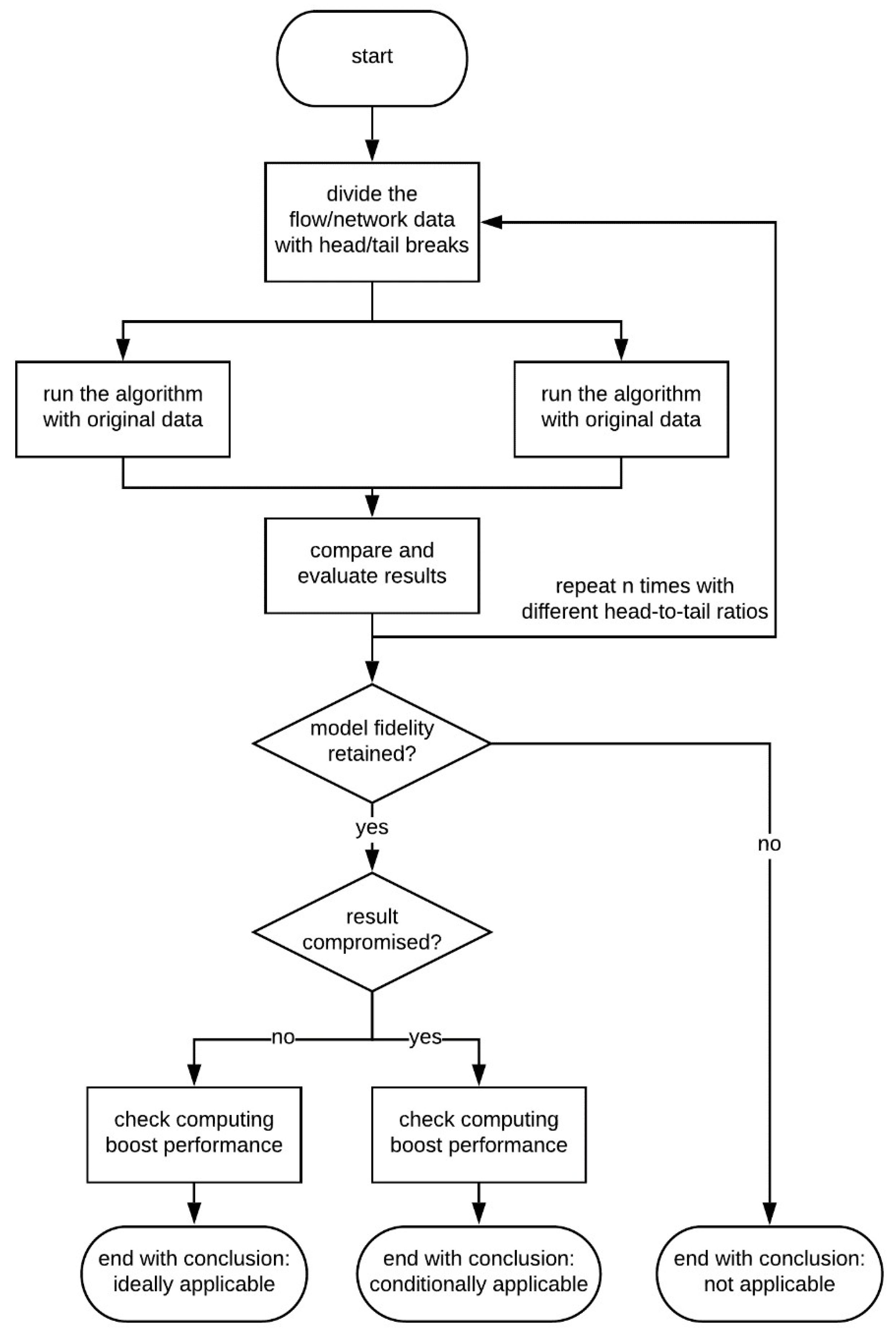
We design an evaluation framework to test the applicability of head/tail breaks to any flow analytics algorithm. As shown in Figure 2, the process begins with splitting the flow data into two parts with head/tail breaks. There are at least two options to set the breakpoint: based on a specific flow value (e.g., mean) or on a preset head-to-tail ratio. The next step is to run the algorithm with the original data and with the “head” part only, respectively. Then we record the computing time and algorithm results of each test and repeat the process with different head-to-tail ratios. Even though the main purpose of head/tail break data reduction is to boost the computational efficiency of the algorithm, the bottom line is that model fidelity has to be maintained, i.e., the algorithm ought to produce results that are fundamentally consistent with results generated on the original data. The actual way to carry out this step varies according to the type of algorithm. For instance, a clustering algorithm should retain a similar number of clusters, while a ranking algorithm should keep most ranks consistent. If it fails, the whole evaluation process ends with the conclusion that head/tail breaks do not apply innocuously to this particular algorithm, and it becomes meaningless to record the computing performance.

Nevertheless, the assessment of model fidelity may indicate the original results are not perfectly preserved. In practice, it is possible that the quality of results is compromised after applying the head/tail breaks, but the loss in quality is still deemed acceptable to retain model fidelity. It is also possible the results are well kept under certain conditions. Therefore, it is necessary to further examine the results to establish the degree to which result quality may be compromised or the ideal computational conditions. We advocate selecting sample results to conduct an in-depth evaluation with means like geovisualization and possibly expert knowledge.

If the model fidelity is maintained, the last step is to check the computing performance boost and find the optimal head-to-tail ratio that balances result quality and speedup. We do not set a fixed threshold on the computing boost because it is subjective to the user whether the speedup is satisfactory.

4.2. Experiment 1. Flow Clustering Method: FlowAMOEBA

We first test with a flow clustering method called flowAMOEBA [10]. It is a data-driven and bottom-up spatial statistic method for identifying spatial flow clusters of extremely high- or low-value, e.g., anomalously large number of travelers between two regions. This method is an ideal choice to test the effectiveness of head/tail breaks. It includes an iterative process to spatially search clusters of extreme value, which takes a long time to compute even for a relatively small dataset. The algorithm of flowAMOEBA is briefly summarized as follows.

(a)

Identify the neighbor flows of each flow based on the contiguity of both endpoints. For example, the state-to-state migration flow from California to North Carolina can be seen as a flow that is neighbor of the migration flow from California to South Carolina, as they share the same origin while their destinations are contiguous.

(b)

Select an arbitrary flow as the seed of a cluster and calculate its $G_i^{\ast }$ statistic [25,26] with Equation (1). The classical $G_i^{\ast }$ statistic is used to measure the concentration of high or low values at a given location i. The $G_i^{\ast }$ value of the seed flow is taken as the starting point of an iterative cluster-expanding process. The spatial weight $w_{ij}$ is set as 1 if flow j neighbors flow i, otherwise 0. N is the total number of flows. $x_j$ is the value of flow j. $\overline{x}$ is the mean value of all flows. 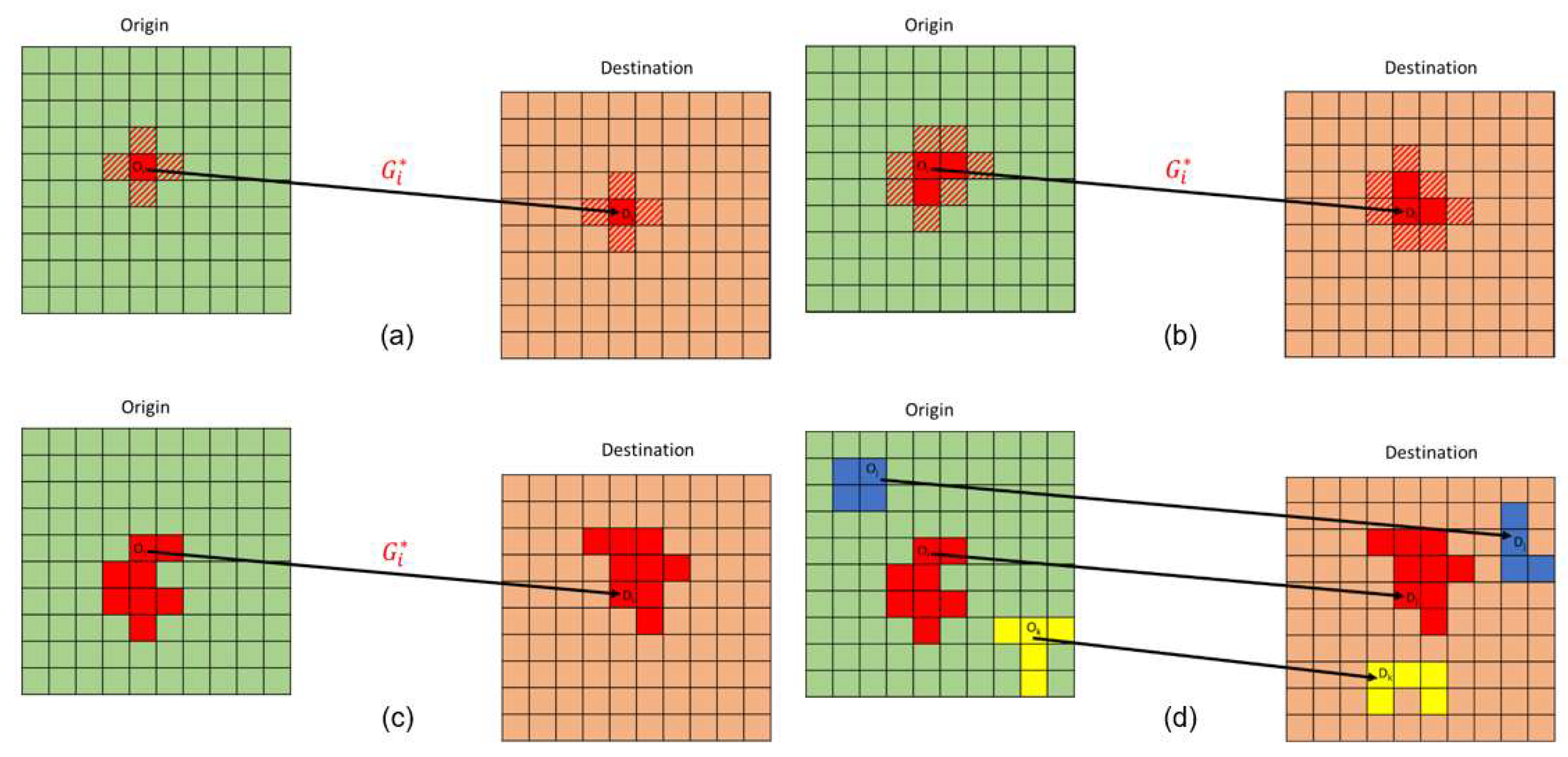Figure 3a shows the selected seed flow and its $G_i^{\ast }$ value, while the grid cells filled with red stripe lines represent the origins and destinations of flow i’s neighbors.

$$\begin{gathered} G_i^{\ast }=({{\displaystyle \sum }}_{j=1}^N{w}_{ij}{x}_j-\overline{x}{{\displaystyle \sum }}_{j1}^N{w}_{ij})/S\sqrt{\frac{N{{\displaystyle \sum }}_{j=1}^N{w}_{ij}{}^2-{{\displaystyle \sum }}_{j1}^N{w}_{ij}{}^2}{N-1}}, \\ \mathrm{where}S=\sqrt{\frac{{{\displaystyle \sum }}_{j=1}^N{x}_j{}^2}{N}-{\overline{x}}^2}. \end{gathered}$$

(1)

(c)

Traverse the neighbor flows of the seed one by one and include the ones that can increase the overall $G_i^{\ast }$ value to the cluster. Figure 3b shows that some of flow i’s neighbors (between solid-filled red grid cells) are selected to merge with the seed as a larger cluster. The algorithm will continue the attempt to absorb more flows through discrimination of the neighbors of the newly joined flows (between the grid cells filled with red stripe lines) with the same criterion.

(d)

Stop the search-and-expand process once the $G_i^{\ast }$ value cannot increase anymore. By then, the flow cluster reaches a stable stage and no more flow neighbors can join. Figure 3c depicts the stable status of the flow cluster regarding seed flow i.

(e)

Repeat the previous three steps and until every flow has served as seed. Collect all flow clusters at their stable stage. Figure 3d illustrates the identified flow clusters originated from different seeds. Conduct a 1000-time Monte-Carlo simulations by randomly permutating the flow values. Preserve the flow clusters that pass the statistical significance level, e.g., 0.01, as the final outcome.

However, the demands of big flow data analysis do not spare the computational capability and efficiency of flowAMOEBA. The most time-consuming part is the iterative search-and-expand process starting from each seed flow. This process is mutually independent from the start at each seed, which means parallel computing techniques can readily be incorporated, similar to how Widener et al. [27] accelerated the original AMOEBA method [28]. Nevertheless, the speedup of flowAMOEBA brought by parallel computing is still underwhelming even with highly capable infrastructure. Here we demonstrate that by applying the head/tail breaks we can achieve a much faster computation without compromising the flow clustering results.

We conduct a test with a flow dataset on inter-city travel in China acquired from Baidu Map Inc. The dataset represents the number of people traveling from one of the 36 cities in Northeast China to one of the 300 cities in the rest of the country at the prefecture-city level on April 1st, 2017. In total, there are 147,416 travelers on that day, encapsulated in 5719 non-zero city-to-city flows. The highest flow value is 4585, which corresponds to the number of travelers from Shenyang (the largest city in Northeast China) to Beijing on that day. The dataset follows a typical heavy-tailed distribution as most flows bear a small value. In total, 96 percent of the flows have a value less than 100, and 80 percent have a value less than 15.

The original computing time is close to 10,419 s or nearly 3 h, of which only 15.8 s were spent on the first step, a task not suitable for multi-core computing. The rest of the steps, including the search-and-expand process from each seed and the 1000-time Monte-Carlo simulations, are ideal for parallel computing. Although we did not conduct this experiment with a highly capable computing infrastructure, the theoretically fastest parallel computing time with 1000 computing cores for the task on hand is about 26.2 s, according to Amdahl’s law [29].

The way we apply head/tail breaks is to preselect some of the highest-value flows, or only the “head” part, as seed flows in the second step. Considering that flowAMOEBA aims at identifying clusters of flows with anomalously high absolute value, it is meaningless to start the computation with those low-value flows which have no chance of being part of a flow cluster. On the other hand, picking a low-value flow as the seed leads to a lengthy expansion process. Since the algorithm keeps searching for relatively higher-value flows to merge with, a humble starting point means more flows would satisfy the criterion, i.e., increasing the overall $G_i^{\ast }$ value. In turn, a large number of flows to join the cluster leads to many more directions for the next search-and-expand step, and so on.

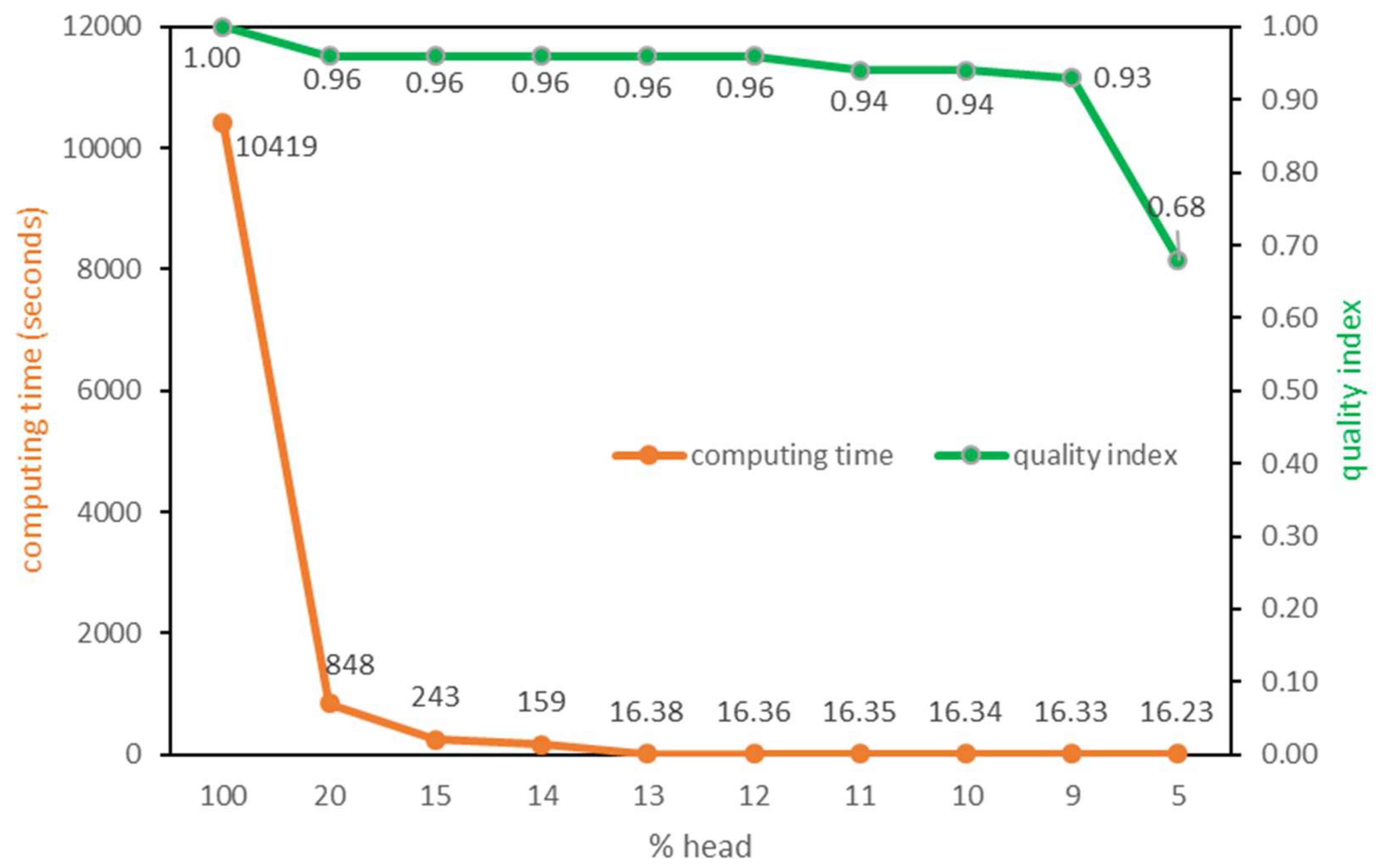
As Figure 4 shows, a series of experiments have been conducted with different breakpoint values. The leftmost starting point denotes the situation when taking the entire dataset into the computing, or without applying head/tail breaks. The computing time decreases dramatically by applying the head/tail breaks to restrict seed flows selection. If selecting the top 20 percent as seeds, the computing time decreases to 848 s. Furthermore, it takes only slightly over four minutes if selecting the top 15 percent as seeds. The computing time keeps diving as the head-to-tail ratio drops. A relatively stable status is reached when the top 13 percent of flows are selected as seeds, since then the computing time stays about 16 s. Considering that 15.8 s are spent on the first step to identify flow neighbors, the actual computing time since the second step has been reduced to less than one second with the help of data reduction by head/tail breaks.

The improvement of the computation is only meaningful with no or very minor compromise of the quality of the results. To evaluate the model fidelity, we design a quality index QI by incorporating the number of detected clusters and the total flow value of the detected clusters, calculated as Equation (2):

$$QI=\frac{N{C}_{ht}\ast V{C}_{ht}}{N{C}_{all}\ast V{C}_{all}}$$

(2)

where NC is the number of detected flow clusters; VC is the total flow value, or the total number of travelers in this example, of the detected clusters. The numerator corresponds to the result by applying head/tail breaks to the seed selection, while the denominator is the result on the whole dataset.

Referring to Figure 4, the quality index remains at a high level in most tests. However, when selecting only the top 5 percent of flows as seeds, the quality index collapses to 0.68. Taking both the computation and the result quality into account, the plausible optimal breakpoint falls at the 13:87 head-to-tail ratio, where the computing time is close to the minimum and the quality index stays above 0.95.

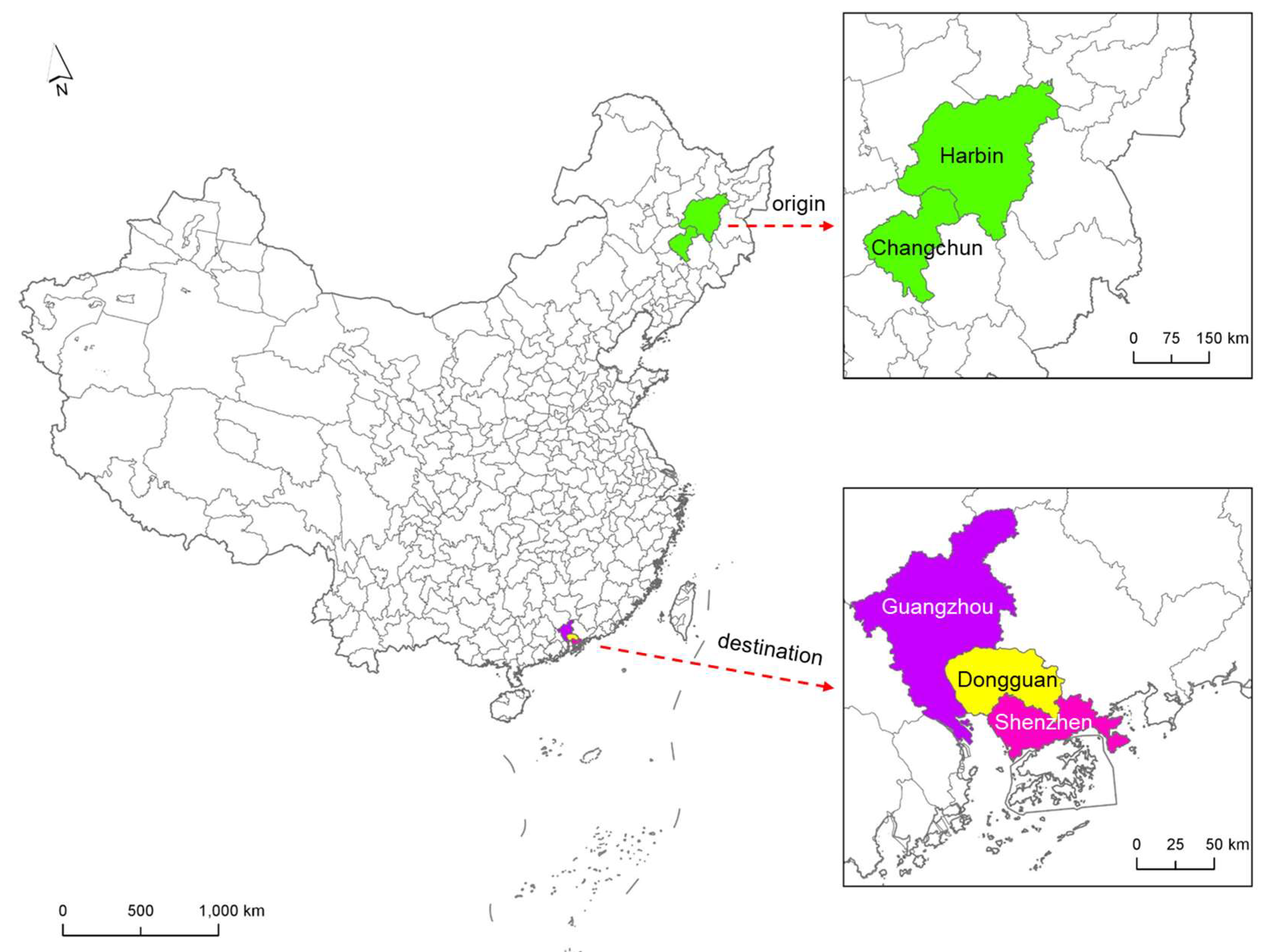
We further examine the differences that head/tail breaks bring to the flowAMOEBA results, which might not be reflected in the quality index. The original result contains 28 flow clusters capturing 81,044 travelers, while the result after applying head/tail breaks at the 13:87 head-to-tail breakpoint contains 27 clusters that capture 81,072 travelers. Through careful comparison of the detail of these two sets of results, we find that the latter includes an additional flow that connects two separate flow clusters in the original result as one bigger cluster. As shown in Figure 5, the original result has two separate clusters between these two regions: Harbin-Changchun to Guangzhou, and Harbin-Changchun to Shenzhen. Instead, the result after applying the head/tail break includes an extra flow from Harbin to Dongguan. Because of the contiguity relationship, this extra flow helps merge the two separate clusters of the original solution as one. Therefore, the number of detected clusters decreases by one, and the total flow value of the clusters increases by 28, which is the value of the additional flow. A possible reason behind this change is that the flow from Harbin to Dongguan barely passes the threshold set by the head/tail breaks to qualify as a seed flow. The search-and-expand process starting from this flow can easily include the nearby flows of higher value and pass the significance test. On the contrary, this same flow is likely to join a cluster through a search-and-expand process that started from a low-value flow, which leaves the cluster a lower chance to pass the significance test.

This further examination of the result differences reveals a fact that a similarity-based quality index cannot convey. The cluster “missing” after applying head/tail breaks is due to the inclusion of an extra flow. This slight difference of the results after applying head/tail breaks to flowAMOEBA falls short of implying the result quality is compromised. On the other hand, the improvement on the computing time is so large that computing time is much less than the theoretically fastest scenario with 1000 computing cores in parallel.

4.3. Experiment 2. Network Community Detection Method: Louvain

As stated earlier, spatial flows can be regarded as the edges of a network. Head/tail breaks and network community detection methods can be a great combination [16]. In the second experiment, we conduct a test with the Louvain method [5], which is a widely-adopted algorithm to extract community structures from large networks. The reasons for selecting Louvain are twofold: the method itself is well-accepted in both industry and academia, and it weighs the weight and direction of edges (flows) to detect communities. The Louvain algorithm is one of the fastest modularity-based algorithms that suit large networks. It is built on the modularity index calculated as Equation (3), which is a scalar value between −1 and 1 that measures the density of edges inside communities as compared to edges between communities [5].

$$Q=\frac{1}{2m}{{\displaystyle \sum }}_{i,j}\left[A_{ij}-\frac{k_i{k}_j}{2m}\right]\delta \left(c_i,c_j\right),$$

(3)

where $A_{ij}$ is the weight of edge (flow) between i and j; $k_i$ is the sum of edge (flow) weights attached to node i, respectively; m is the sum of all edge (flow) weights in the network; $c_i$ is the community that includes node i; $\delta \left(c_i,c_j\right)$ equals 1 if u = v, and 0 otherwise.

The algorithm initializes each node as its own community. In the first step, each node is switched from its current community to one of its neighbors’ community. The switch is confirmed if it helps increase the modularity value. This process is applied repeatedly for all nodes until no further improvement can be achieved, in other words, a local maximum of the modularity is reached. The second step is to define a new coarse-grained network, whose nodes are the communities found in the first step. The edge weights between the new nodes are the sum of the edge weights between the lower-level nodes of each community. These two steps are repeated until no further modularity-increasing reassignments of communities can be found.

We apply head/tail breaks to Louvain to reduce the input data to the “head” part of the distribution only. We test with a large cellphone call flow dataset in the Beijing-Tianjin-Hebei (BTH) urban agglomeration in China in November 2017. Each flow event represents a cellphone call made from one location to another. They are aggregated to the basic spatial units as one-kilometer-by-one-kilometer grid cells. After aggregation, the dataset consists of 45 million flows that connect 177,608 grid cells. The dataset is extremely heavy-tailed: a flow value of 5 or more places a dyad in the top 10.8% of the entire dataset. We test with a series of head/tail breaks to record the computing times while evaluating the results. Because the Louvain algorithm assigns every grid cell to a community, many resulting communities end up with one or just a few cells. To evaluate the result quality, we focus on the meaningful big communities while ignoring the noisy small ones. Since the definition of big communities can be arbitrary, we pick out the 100 largest communities of every test to have consistent cross-comparisons. Specifically, we compare the population sizes of these communities and their spatial patterns through visualization. We adopt the publicly available population data from www.worldpop.org to count the population within the communities, specifically we use the 2015 Asia population dataset in 1 km resolution.

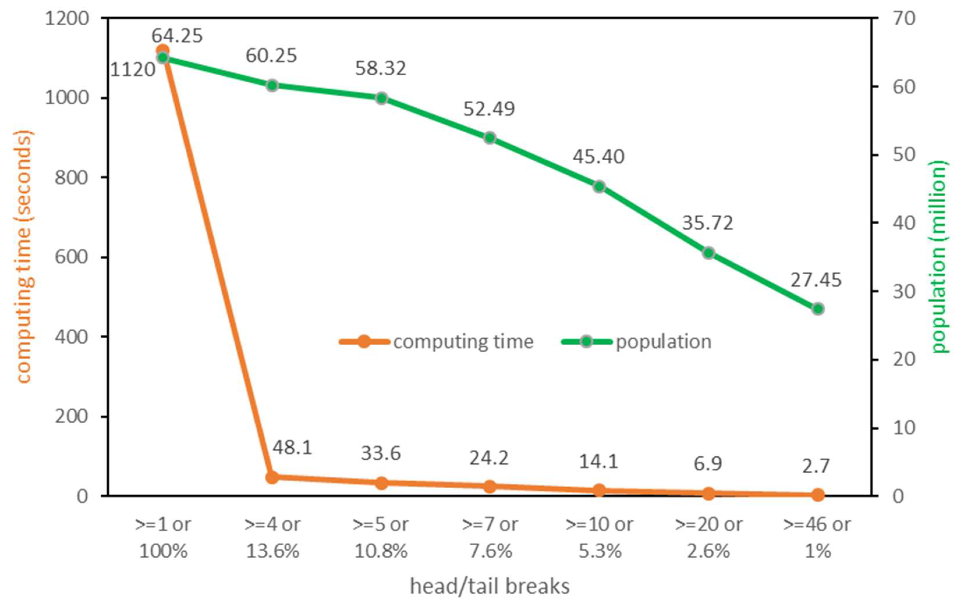
Figure 6 summarizes the test results. The original computing time is 1120 s without applying head/tail breaks. It is decreased to 48.1 s by selecting the flows with value equal or larger than 4, or the top 13.6%, as input data. The computing time can be further shrunk with lower head-to-tail ratio. For instance, it would take less than half a minute to process only the top 1% as the input data.

On the other hand, the total population of the 100 largest communities of each test has decreased to some extent as the head-to-tail ratio lowers. Taking the top 10.8% flows as the input data, the algorithm keeps a population of 58.32 million in the 100 largest generated communities. Although the shrinking of community sizes is expected, the degree of shrinking is conservative as 90.8% of the original population are kept.

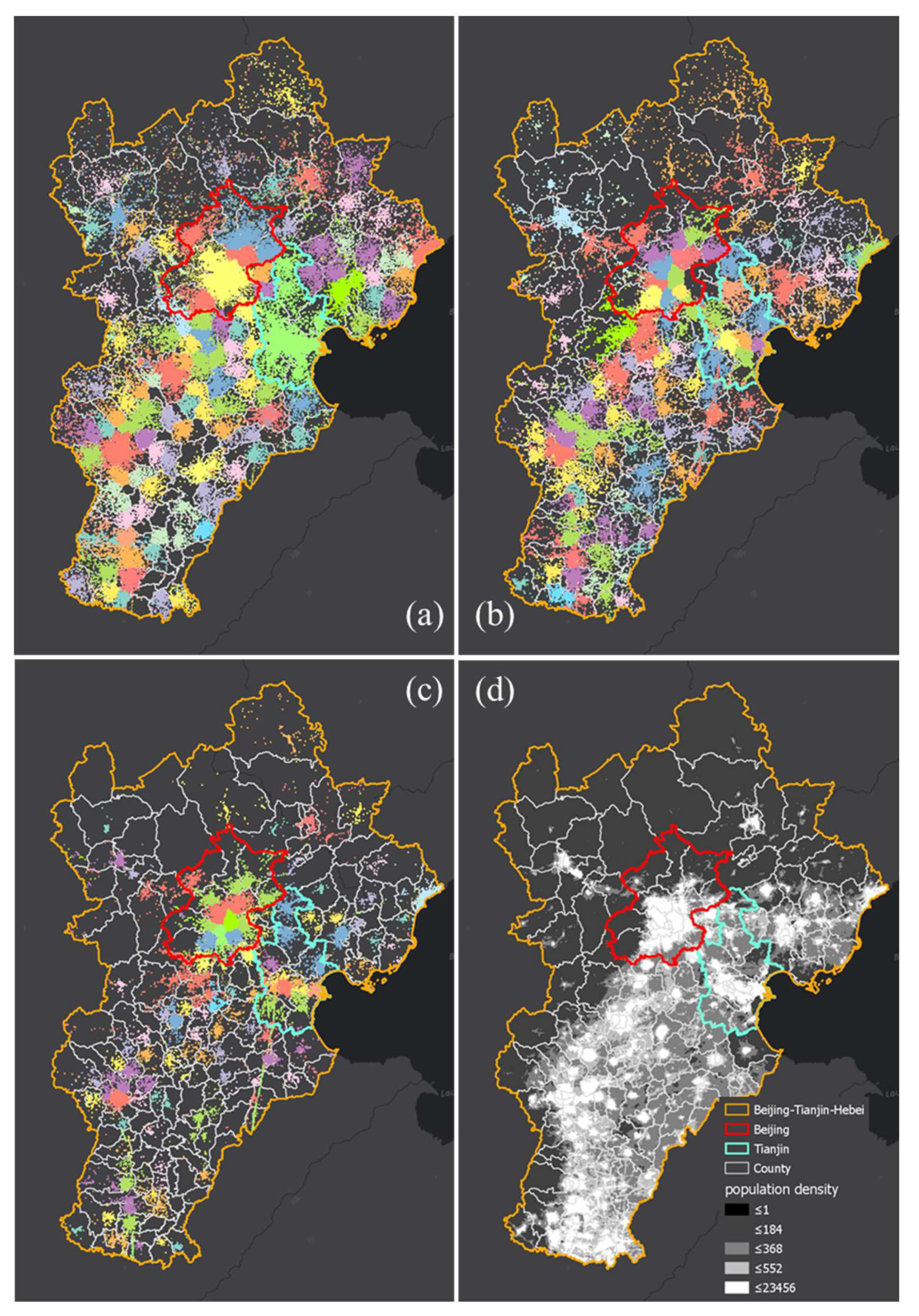
To further examine the effect of applying head/tail breaks on the results, we visualize three sets of detected communities as well as the population density in the study area as Figure 7. Only the 100 largest communities of each test are visualized with a qualitative color scheme, while the rest of the grid cells are hidden as noise. The colors differentiate the communities of the same map, but there is no correspondence relationship of the same color across the maps. Several observations can be made.

First, all the tests can extract at least a hundred unique communities at a granularity commensurate with counties. Most detected communities are consistent with the predefined county boundaries, with a few exceptions that are formed by multiple neighboring counties. Second, applying head/tail breaks to selectively reduce the input data would shrink the spatial extent of the retained communities within the BTH urban agglomeration. Comparing with the population density map in Figure 7d, we see that the shrunk communities preserve the most populous core regions, while losing the peripheral grid cells. Relating back to the chart in Figure 6, it can be concluded that the significant shrinking of communities’ spatial extent on the map does not lead to a proportional decrease of the population encompassed by these communities. In other words, the results obtained with head/tail breaks preserve the most meaningful parts of the community structures. Last but not least, head/tail breaks can help extract communities at lower hierarchical level. In Figure 7a, Beijing (with red outline) consists of a few communities and Tianjin (with turquoise outline) is detected as a single large community. By applying head/tail breaks, both megacities can be decomposed into a number of smaller communities that correspond to the city districts. This change probably results from the data reduction produced by the head/tail breaks that filter out the low-value flows that serve as the weak links between city districts. With only the “head” part as the input data, the algorithm is better positioned to extract the spatially compact communities with strong internal cohesion.

To sum up, through this series of experiments with the classical Louvain algorithm, we found that the data reduction method of head/tail breaks can significantly boost the computation on large flow/network dataset. The computing time keeps decreasing as the head-to-tail ratio is set lower. However, beyond a certain point, it becomes less appealing to save a few extra seconds at the expense of degraded geographic representation of communities. The plausible optimal threshold of flow value in this case falls between 4 and 5, corresponding to the top 13.6% and 10.8% as the “head”, respectively.

4.4. Experiment 3. Network Centrality Algorithm: PageRank

In this section, we test a well-known network centrality algorithm, namely weighted PageRank (WPR; [8]), which is a link analysis method to measure centrality of nodes in a graph. By considering the importance of links, the WPR is an extension of the original PageRank algorithm developed by Google to rank the relative importance of website pages [30]. As spatial flows between locations can be represented by directed and weighted edges (links) of a network dataset, WPR has been used to measure the relative attractiveness or importance of locations in spatial interaction contexts involving various spatial flows [6,7]. The WPR algorithm follows an iterative process by which the WPR value of each node is continuously calculated until convergence is reached. For a node $v_i$ in a network of $N$ nodes, the WPR value of $v_i$ is computed as follows:

$$WPR\left(v_i\right)=\frac{1-d}{N}+d{{\displaystyle \sum }}_{v_j\in K\left(v_i\right)}\frac{w_{j,i}}{{{\displaystyle \sum }}_i^N{w}_{j,i}}WPR\left(v_j\right)$$

(4)

where $d$ is the residual probability which is fixed by an empirically estimated value 0.85; $K\left(v_i\right)$ is the set of nodes that have outbound links to $v_i$; $w_{j,i}$ is the weight (or flow value) of an outbound link from $v_j$ to $v_i$. During calculating, the first term $\frac{1-d}{N}$ in Equation (4) is fixed and thus $WPR\left(v_i\right)\propto {\displaystyle \sum }_{v_j\in K\left(v_i\right)}\frac{w_{j,i}}{{{\displaystyle \sum }}_i^N{w}_{j,i}}WPR\left(v_j\right)$, which means the WPR value for a node in question is dependent on a sum of the weighted WPR values of all other nodes that have outbound links to this node. The weighting term is the weight ($w_{j,i}$) of an outbound link normalized by the sum of weights for all outbound links from a node $v_j$. Firstly, due to the normalization, weighting becomes relative and the absolute flow values (link weights) become not meaningful to the final WPR values anymore, which hypothetically contradicts the basic assumption of head/tail breaks that the links (flows) with larger weights carry more value in the results of analysis. Second, according to the fundamental assumption of the WPR algorithm that more important nodes (higher WPR values) are likely to receive a larger number of links from other nodes that are also important, link distribution instead of weight distribution plays a major role in affecting WPR values. That is, the concentration of incoming links (e.g., larger node in-degree) causes larger sizes of $K\left(v_i\right)$ and $\frac{w_{j,i}}{{{\displaystyle \sum }}_i^N{w}_{j,i}}$, and thus larger WPR values. The above hypotheses are tested empirically as follows.

To empirically test the applicability of the head/tail breaks to the weighted PageRank algorithm, the break is applied to the mean value of the weight distribution so that the links with lower weight values are removed from the networks. In a related work, Jiang [6] applied head/tail breaks to handle the heavy-tailed WPR values, which is different from what we are testing here: using head/tail breaks to select link values (reduce input data) and see if the WPR values can be retained. Therefore, the model fidelity can be evaluated by the degree to which the ranking of WPR values of nodes can be preserved in the reduced network, compared to that of the original network. Specifically, a preservation ratio for the top-$m$% nodes with the highest WPR values between the reduced and the original networks is defined as:

$$P_m=\frac{l_m}{N_m}$$

(5)

where $l_m$ is the number of nodes preserved in the top-$m$% ranked nodes for the reduced network, compared to the number $N_m$ of top-$m\%$ ranked nodes of the original network. By varying the value of $m$, comparison of results can be evaluated for different top-$m$% ranked nodes.

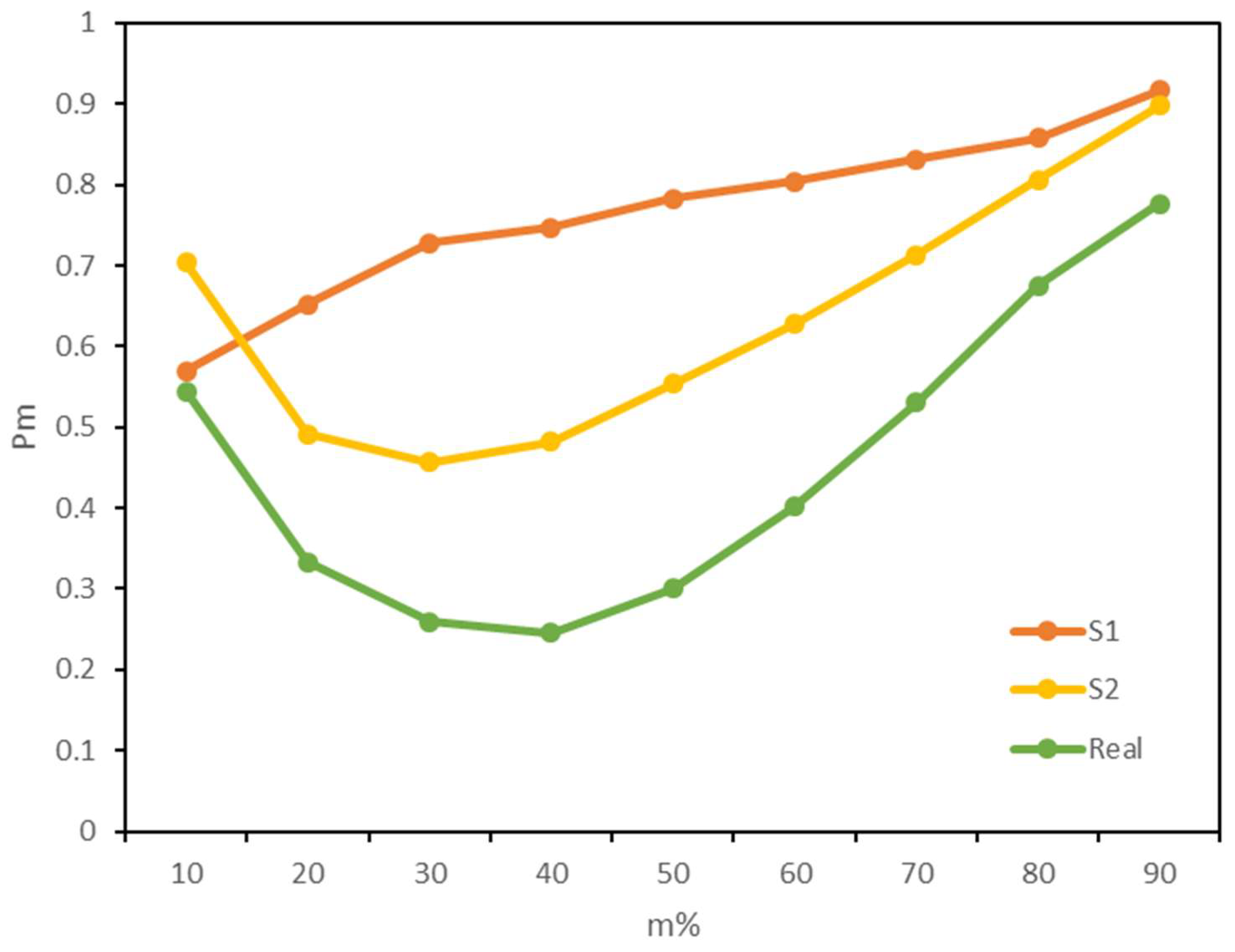
We test with the same cellphone call flow dataset for the Beijing-Tianjin-Hebei (BTH) urban agglomeration used in Experiment 2. Figure 8 shows the preservation ratios for this dataset (Real) for a range of top-$m$% ranked nodes. It exhibits rather lower preservation ratios over the entire range of $m$%. Specifically, only half of the top 10% ranked nodes are preserved, and then the preservation ratio decreases at the lowest for $m$%=40% and increases again for $m$% = 50% and higher, which portrays a nonmonotonic trend. As expected, the computing time is reduced from 314 s to 22 s after the head/tail break. However, the performance gain is meaningless given the loss of model fidelity in general. This finding supports our first hypothesis about the contradiction between the weighted PageRank’s relative weighting scheme and the assumption of applying head/tail breaks for data reduction.

To further confirm our finding, two synthetic datasets are designed as benchmarks to remove the sensitivity due to the choice of test data. The two synthetic datasets are specified as follows. First, a random directed network is created with 100 nodes and 1000 edges that are randomly distributed following a uniform distribution. The edge weights are generated by following a Zipf distribution [31] to allow the application of the head/tail break and are assigned to edges randomly. Second, another random directed network is created with 100 nodes and 1000 edges. The edge weights are also generated from a Zipf distribution, but larger weights are assigned to outbound links of nodes that have higher degree. Since the two datasets are random networks, 30 runs are conducted to control for the effects of randomness.

The preservation ratios for the synthetic datasets 1 and 2 (S1 and S2 in Figure 8) both show a general loss of model fidelity. For S1, half of the top 10% ranked nodes are preserved, 13 of the top 20% nodes, and this ratio is monotonically increasing as m% increases. This is simply because more nodes can be preserved with a larger number of top-m% nodes considered, which is true especially when m > 50 for all three datasets. For S2, more top-10% nodes are preserved, but the preservation ratio decreases first and then increases at 30%, which portrays a similar overall pattern as the Real dataset. The larger ratio of preservation for top-10% nodes can be attributed to the assignment of weights according to the in-degree of nodes, in which case better connected nodes have larger weights thus their links have a higher chance to be kept. It verifies the second hypothesis that the WPR algorithm values the flow (link) distribution more than the flow value (weight) distribution.

In sum, the results of WPR algorithm are severely compromised after applying head/tail breaks for all three datasets tested and the model fidelity is hardly retained in any sensible way. Although conditions where the weight distribution matches the link distribution of nodes could potentially enhance the preservation of original WPR results, the capacity is in fact very limited (for top-10% nodes) in our findings. The empirical tests with three datasets support that the emphasis of weighted PageRank algorithm on relative weighting and link distribution violates the assumption of head/tail breaks and thus renders this algorithm a poor choice for this data reduction technique.

5. Discussion and Conclusions

In this paper, we introduce a solution to the computational challenge of big flow data analytics. The solution stems from a thorough understanding of flow data characteristics, instead of an application of the latest computing infrastructures and techniques. Given that most flow data follow a heavily-tailed distribution, we integrate the practice of data reduction in the existing analytical methods to achieve the computational boost. Specifically, data reduction is based on the notion of head/tail breaks.

We select three algorithms from different method families to test on various datasets. As summarized in

Table 1. Summary of results.

Algorithm	Method Family	Optimal Head Ratio	Computational Boost	Result Quality	Applicability of Head/Tail Breaks
flowAMOEBA	flow clustering	13%	636 times	satisfactory	ideal
Louvain	community detection	10.8%	33 times	conditionally satisfactory	conditional
weighted PageRank	network centrality	N/A	N/A	unacceptable	N/A

, the experiment results demonstrate the effectiveness of our solution, while also narrowing down the suitable application conditions. First, we found that the head/tail breaks approach is ideally applicable to the flow clustering method flowAMOEBA, as it does not compromise the result quality while achieving a significant improvement in computation time. For the community detection algorithm Louvain, the head/tail breaks approach is conditionally applicable: it significantly boosts the computation, but the results are satisfactory only when the emphasis is on the cores of original communities rather than the peripheral parts. The third experiment with the weighted PageRank, however, does not preserve the ranking of the nodes consistently, despite the computing time reduction. The reason is that the weighted PageRank emphasizes the link distribution and the relative weights of the links rather than the absolute weights, while only the latter exhibits a heavy-tail distribution that the head/tail breaks can take advantage of.

To sum up, the data reduction by head/tail breaks can be integrated effectively with some of the existing flow analytical methods to significantly improve the computation. The solution is easy to implement: selecting the “head” part of the data before or during performing the algorithm. The computational improvement is very promising and is often superior to the boost directly obtained with parallel computing on a capable computing infrastructure. However, the applicability of head/tail breaks is conditional, as the experiment with the weighted PageRank disproves its universal applicability. In other words, the application of head/tail breaks is subject to the condition that the algorithm emphasizes on the “head” part of the flow dataset sorted by the absolute flow values (link weights). In addition, it is important to bear in mind that the types of spatial flow data analysis that can benefit from data reduction through head/tail breaks are not limited to the representative algorithms that we tested, or the method families of flow clustering, community detection, or network centrality. Any method that can take advantage of the heavy-tailed distribution may benefits from the head/tail breaks method. With the evaluation framework we proposed here, the applicability and effectiveness of head/tail breaks can be easily and systematically evaluated for any ad hoc method.

There are at least four directions for future research. First, since the heavy-tailed distribution is prevalent in many cases of big data, not just in flow data, the applicable domain of head/tail breaks can certainly be expanded to other types of methods. Second, the “head” part of the distribution is not always the study focus; therefore, the potential for exploiting the “tail” should be explored in situations such as detecting “cold spots” as outliers or removing the “head” as noise. Third, the notion of head/tail breaks should be evaluated for efficacy against other data reduction. Last but not least, combining the solution presented here with the latest computing infrastructure or techniques is a promising way to achieve even greater computational boost.

References

1. Farmer, C.; Oshan, T. Spatial interaction. In The Geographic Information Science & Technology Body of Knowledge, 4th Quarter 2017 ed.; Association of American Geographers: Washington, DC, USA, 2017. [Google Scholar]
2. Tao, R.; Depken, C.; Thill, J.C.; Kashiha, M. flowHDBSCAN: A hierarchical and density-based spatial flow clustering method. In Proceedings of the 3rd ACM SIGSPATIAL Workshop on Smart Cities and Urban Analytics; ACM: Redondo Beach, CA, USA, 2017; p. 11. [Google Scholar]
3. Batty, M. The new Science of Cities; MIT Press: Cambridge, MA, USA, 2013. [Google Scholar]
4. Gao, S.; Liu, Y.; Wang, Y.; Ma, X. Discovering Spatial Interaction Communities from Mobile Phone Data. Trans. GIS 2013, 17, 463–481. [Google Scholar] [CrossRef] [Green Version]
5. Blondel, V.D.; Guillaume, J.L.; Lambiotte, R.; Lefebvre, E. Fast unfolding of communities in large networks. J. Stat. Mech. Theory Exp. 2008, 2008, 1–12. [Google Scholar] [CrossRef] [Green Version]
6. Jiang, B. Ranking spaces for predicting human movement in an urban environment. Int. J. Geogr. Inf. Sci. 2009, 23, 823–837. [Google Scholar] [CrossRef] [Green Version]
7. Chin, W.C.B.; Wen, T.H. Geographically modified PageRank algorithms: Identifying the spatial concentration of human movement in a geospatial network. PLoS ONE 2015, 10, e0139509. [Google Scholar] [CrossRef] [PubMed]
8. Xing, W.; Ghorbani, A. Weighted pagerank algorithm. In Proceedings of the Second Annual Conference on Communication Networks and Services Research, Fredericton, NB, Canada, 21–21 May 2004; pp. 305–314. [Google Scholar]
9. Broido, A.D.; Clauset, A. Scale-free networks are rare. Nat. Commun. 2018, 10, 1–10. [Google Scholar] [CrossRef] [PubMed]
10. Tao, R.; Thill, J.C. flowAMOEBA: Identifying Regions of Anomalous Spatial Interactions. Geogr. Anal. 2019, 51, 111–130. [Google Scholar] [CrossRef]
11. Clauset, A.; Shalizi, C.R.; Newman, M.E.J. Power-law distributions in empirical data. SIAM Rev. 2009, 51, 661–703. [Google Scholar] [CrossRef] [Green Version]
12. Roy, J.R.; Thill, J.-C. Spatial interaction modelling. Pap. Reg. Sci. 2003, 83, 339–361. [Google Scholar] [CrossRef]
13. Jiang, B. Head/Tail Breaks: A New Classification Scheme for Data with a Heavy-Tailed Distribution. Prof. Geogr. 2013, 65, 482–494. [Google Scholar] [CrossRef]
14. Jiang, B. Head/tail breaks for visualization of city structure and dynamics. Cities 2015, 43, 69–77. [Google Scholar] [CrossRef] [Green Version]
15. Jiang, B. A recursive definition of goodness of space for bridging the concepts of space and place for sustainability. Sustain. Switz. 2019, 11, 4091. [Google Scholar] [CrossRef] [Green Version]
16. Jiang, B.; Ma, D. Defining least community as a homogeneous group in complex networks. Phys. Stat. Mech. Its Appl. 2015, 428, 154–160. [Google Scholar] [CrossRef] [Green Version]
17. Long, Y.; Zhai, W.; Shen, Y.; Ye, X. Understanding uneven urban expansion with natural cities using open data. Landsc. Urban Plan. 2018, 177, 281–293. [Google Scholar] [CrossRef] [Green Version]
18. Gong, Z.; Ma, Q.; Kan, C.; Qi, Q. Classifying Street Spaces with Street View Images for a Spatial Indicator of Urban Functions. Sustainability 2019, 11, 6424. [Google Scholar] [CrossRef] [Green Version]
19. Tobler, W.R. Experiments in migration mapping by computer. Am. Cartogr. 1987, 14, 155–163. [Google Scholar] [CrossRef] [Green Version]
20. ur Rehman, M.H.; Liew, C.S.; Abbas, A.; Jayaraman, P.P.; Wah, T.Y.; Khan, S.U. Big Data Reduction Methods: A Survey. Data Sci. Eng. 2016, 1, 265–284. [Google Scholar] [CrossRef] [Green Version]
21. Li, Y.; Li, T.; Liu, H. Recent advances in feature selection and its applications. Knowl. Inf. Syst. 2017, 53, 551–577. [Google Scholar] [CrossRef]
22. Arnaiz-González, Á.; Díez-Pastor, J.F.; Rodríguez, J.J.; García-Osorio, C. Instance selection of linear complexity for big data. Knowl.-Based Syst. 2016, 107, 83–95. [Google Scholar] [CrossRef] [Green Version]
23. Czarnowski, I.; Jędrzejowicz, P. Learning from examples with data reduction and stacked generalization. J. Intell. Fuzzy Syst. 2017, 32, 1401–1411. [Google Scholar] [CrossRef]
24. Olvera-López, J.A.; Carrasco-Ochoa, J.A.; Martínez-Trinidad, J.F.; Kittler, J. A review of instance selection methods. Artif. Intell. Rev. 2010, 34, 133–143. [Google Scholar] [CrossRef]
25. Getis, A.; Ord, J.K. The Analysis of Spatial Association by Use of Distance Statistics. Geogr. Anal. 1992, 24, 189–206. [Google Scholar] [CrossRef]
26. Ord, J.K.; Getis, A. Local Spatial Autocorrelation Statistics: Distributional Issues and an Application. Geogr. Anal. 1995, 27, 286–306. [Google Scholar] [CrossRef]
27. Widener, M.J.; Crago, N.C.; Aldstadt, J. Developing a parallel computational implementation of AMOEBA. Int. J. Geogr. Inf. Sci. 2012, 26, 1707–1723. [Google Scholar] [CrossRef]
28. Aldstadt, J.; Getis, A. Using AMOEBA to Create a Spatial Weights Matrix and Identify Spatial Clusters. Geogr. Anal. 2006, 38, 327–343. [Google Scholar] [CrossRef]
29. Amdahl, G.M. Validity of the single processor approach to achieving large scale computing capabilities. In Proceedings of the AFIPS Spring Joint Computer Conference, Atlantic City, NJ, USA, 18–20 April 1967; pp. 483–485. [Google Scholar]
30. Page, L.; Brin, S. The anatomy of a large-scale hypertextual Web search engine. Comput. Netw. 1998, 30, 107–117. [Google Scholar]
31. Zipf, G.K. Selected Studies of the Principle of Relative Frequency in Language; Harvard Univ. Press: Cambridge, MA, USA, 1932. [Google Scholar]
Figure 1. Heavy-tailed distribution of U.S. migration flows.
Ijgi 09 00299 g001
Figure 2. Evaluation framework flowchart.
Ijgi 09 00299 g002
Figure 3. Different stages of the flow cluster expansion: (a) starting from a seed flow (b) flow cluster enlarged but still expanding (c) stable stage of one flow cluster. (d) stable stage of multiple flow clusters regarding different seed locations.
Ijgi 09 00299 g003
Figure 4. Performance of flowAMOEBA with head/tail breaks.
Ijgi 09 00299 g004
Figure 5. Flow cluster from Northeast China to the Pearl River Delta.
Ijgi 09 00299 g005
Figure 6. Performance of Louvain with head/tail breaks.
Ijgi 09 00299 g006
Figure 7. Communities detected with Louvain using (a) 100% (b) top 10.8% (c) top 5.3% of the cellphone call flow data. (d) Population density visualized with quantile classification of the same Beijing-Tianjin-Hebei (BTH) region.
Ijgi 09 00299 g007
Figure 8. The preservation ratios (Pm) calculated for one read-world dataset (Real) and two synthetic datasets (S1 and S2).
Ijgi 09 00299 g008