Multi-Scale Representation of Ocean Flow Fields Based on Feature Analysis

Abstract

When it comes to feature retention in multi-scale representations of ocean flow fields, not all data points are equal. Therefore, this paper proposes a method of selecting data points based on their importance. First, an autocorrelation analysis is performed on flow speed and the rate of change in flow direction. Then, the magnitude of speed and variation in the rate of change in flow direction are classified. Feature regions are determined according to autocorrelation aggregation and classification analysis. Then, rough set theory and evidence theory are applied, using these results to determine the weights of different points. Finally, these weights are used to construct multi-scale representations of ocean flow fields, which effectively retain flow-field characteristics.

1. Introduction

With recent advancements in data acquisition technology, the range and resolution of ocean flow field data being collected have both increased significantly, leading to a large amount of data with dense vector points [1,2]. Displaying all of the information contained in dense vector points on a large scale is not only tedious and difficult, but also leads to visualizations that are congested with an overabundance of map symbols. To avoid congestion, multi-scale representations of ocean flow fields must rely on a sample of the available data points, and the size of this sample must vary according to scale. Points in the flow fields have different attributes and relative importance. Some points offer information which is very similar to that of adjacent points, which means that they contribute less information to the flow field overall, while others contain important feature information, which means that they contribute more to the overall characteristics of the flow fields. This critical information about flow field features can be easily missed if the data points are thinned by an equidistant thinning method, or system sampling. Though a comprehensive analysis, the data points can be assigned different weights, which reflect their relative importance and information content, and this can greatly improve the quality of multi-scale flow field representations [3].

Sampling data based on the features of flow fields involves the selection of subsets, structure analysis, feature detection, and accounting for the user’s region of interest within the original dataset [4]. This process can significantly reduce the amount of data points by filtering out uninteresting data. It can not only ensure that important flow field features are visualized effectively, but also improve rendering efficiency. In 1991, Helman et al. proposed a method of extracting vector field topology by identifying and classifying first-order singular points and then applying the method to high-order singular points in order to realize the visualization of nonlinear vector field topologies. Leeuw et al. used multiple levels of topology to carry out the visualization of global flow structure by removing the small-scale topological structure [5]. The chaotic phenomenon is easy to appear when visualizing the large-scale turbulent high-resolution data set. Tricoche et al. studied the visualization of two-dimensional time-varying vector fields based on topology [6]. The critical points and closed streamlines are tracked by the difference value, and topological events can be found and represented. The visualization of the nonlinear vector field topology extends the range of automatically extracted features to relatively fine features in the flow field, such as slow vortices, and can quantitatively describe feature attributes [7,8,9]. The two-dimensional vector field topology includes critical point analysis and topological boundary extraction, which has had a mature development as the key research object of certain researchers [10,11,12]. Physical feature-based extraction takes into account the fact that each feature has independent and direct definition patterns and different methods can be used according to different definitions, e.g., vortex extraction, shock extraction, and line-in-line extraction [13], William proposed an adaptive extraction method based on the Q method [14], which was studied by the distribution of the Q value in the ideal vortex model, the Q value is the difference between tension tensor and vorticity model. It was found that there is an approximate linear relation between the change in the Q value from the vortex kernel point along the radius direction and the radius square. Others—for example, Koehler et al.—studied the visibility of ultra-low Reynolds number vortices around the wings of insects in flight [15], Sadlo et al. proposed a method for Efficient Visualization by Filtered AMR Ridge Extraction [16] and Lipinski et al. developed a ridge tracking algorithm for the computation and extraction of Lagrangian coherent structures (LCS) [17]. These methods are good for extracting the characteristics. Feature extraction based on interaction selection refers to selecting a grid point that satisfies a defined condition by defining a logical expression and extracting the part of the data field which is of interest to the user as a feature [18]. These methods train the neural network by using the region selected by the user as a sample, and the neural network, after training, is used to identify the new data, including an intelligent feature extraction algorithm based on a BP(Back Popagation) neural network proposed by Xu Huaxun et al. and an interactive fuzzy feature extraction algorithm designed to extract features and solve the problem of precisely defining a complex flow field feature region proposed by Shen et al. [19,20].

In general, topology-based feature extraction is good for the extraction of critical points and boundaries. The method can carry out a very precise extraction of a feature based on physical attributes, while the user interaction can better obtain the data needed by the user. Although the feature extraction methods of the flow field have made great progress, most of the methods need to accurately locate the features and the calculation is complex. Generally, the data are the global flow field and other large vector fields in ocean flow visualization. The complex calculation in large vector fields will reduce the efficiency of visualization, and single feature extraction will make feature extraction incomplete. For data sampling, the results of the equidistant sampling method usually make the selected data produce errors [21], and the results of stratified sampling are usually to satisfy users’ understanding of the overall situation, without any emphasis on features.

In order to satisfy the feature extraction of large vector fields and ensure the sampling accuracy of the data, this paper proposes a multi-scale representation method of ocean flow fields based on feature analysis. First, we performs an autocorrelation analysis and classification analysis based on rates of change in speed and direction across the data points in the flow field in order to calculate the weight of each data point with respect to each attribute and extracted feature area. Then, rough set theory is applied to determine the support of each attribute to the feature, and evidence theory is used to determine the weight combination of each attribute. Finally, the points are sampled according to this weight, which reflects how well they represent the flow field feature of interest. The method does not require complex mathematical calculations and uses more stringent conditions to thin out the data. The flow chart of the method is shown in Figure 1:

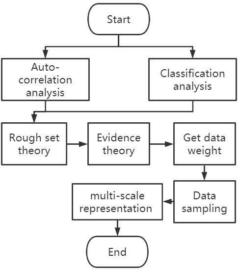
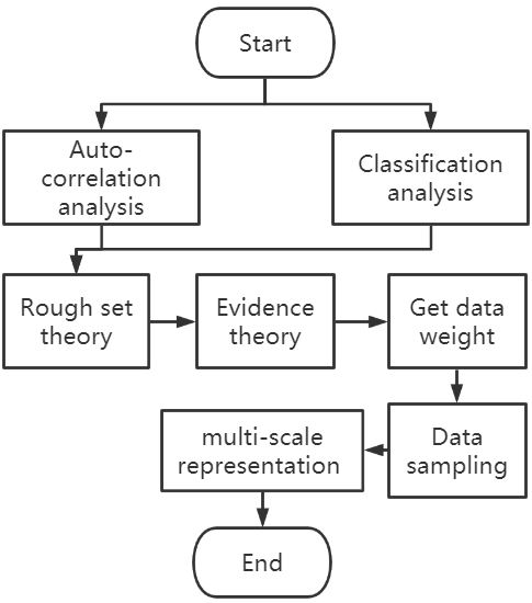
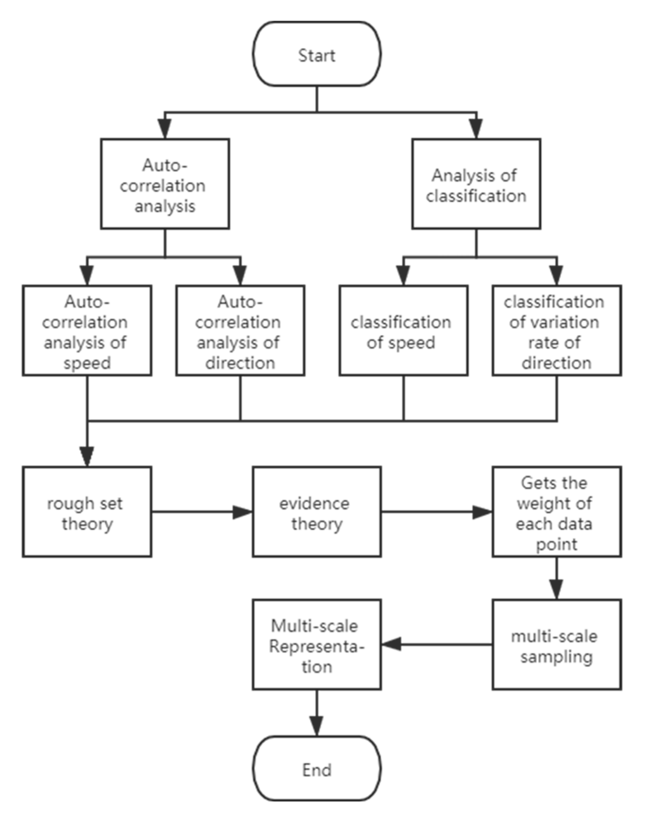
2. Analysis of Attributes, Feature of Flow Fields, and Weight Allocation

Simplifying data by an equidistant thinning method results in missing critical features of flow fields and emphasizing unimportant features. In order to ensure that sampled data points can express the feature information of the flow field as well as possible, this paper proposes the use of autocorrelation analysis to weight data points based on two different types of feature information: flow speed and flow direction.

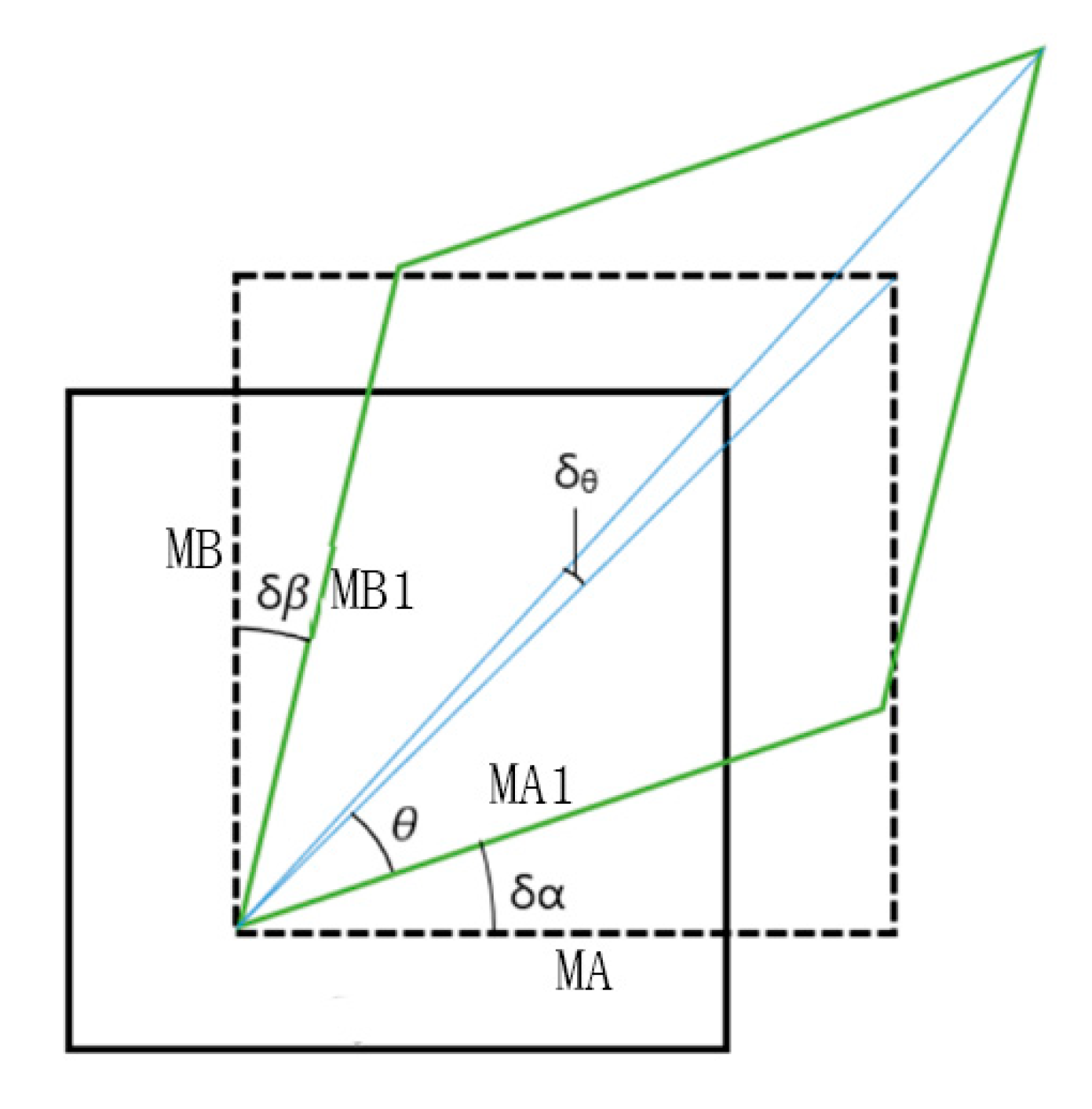
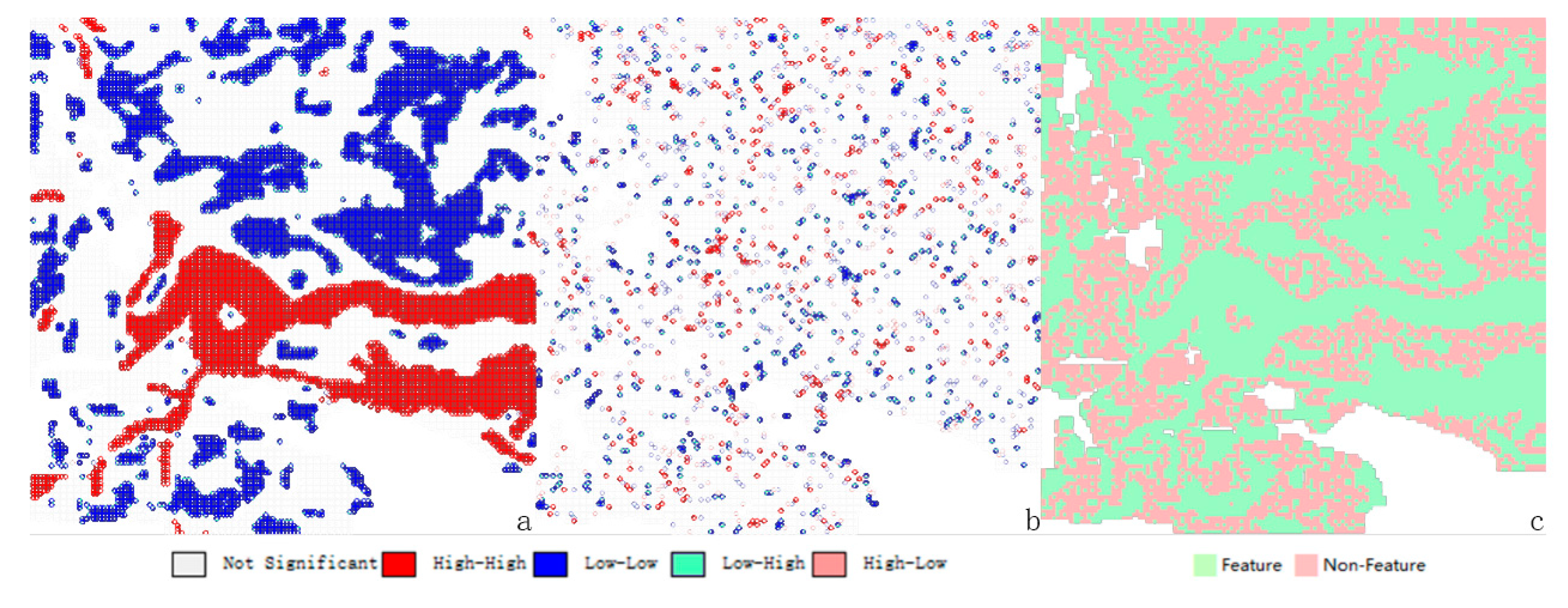
2.1. Autocorrelation Analysis

Spatial autocorrelation is measured based on both feature locations and feature values simultaneously by using global Moran’s I. Spatial autocorrelation can be divided into positive spatial autocorrelation and negative spatial autocorrelation. Positive spatial autocorrelation indicates that spatial phenomena at an observed point have values similar to those of other points in its vicinity. Negative spatial autocorrelation indicates that spatial phenomena values at the points are different from those of other points in the vicinity.

This paper selects a distance-based spatial weight matrix. In order to judge whether there is spatial aggregation, this paper chooses a threshold distance pattern and sets up a distance threshold [22].

2.1.1. Autocorrelation Analysis of Speed

Speed is an important feature of ocean currents. Autocorrelation analysis is used to determine the aggregation pattern of ocean current speed, and the weights of different aggregation patterns are determined through the analysis results. High–low and low–high aggregation correspond to negative spatial negative correlation. High–low aggregation means that the attribute values suddenly decrease, while low–high aggregation means that values suddenly increase, such as when the speed of flow changes from slow to fast. High–high and low–low aggregation corresponds to spatial positive correlation, and describe cases where the flow speed in a region is similar to that in neighboring regions. Weights are allocated according to the relative importance of the speed aggregation mode as it pertains to ocean flow fields. There are five different weights, corresponding to data of no obvious regional relevance, high–high aggregation, low–low aggregation, high–low aggregation, and low–high aggregation, as described in Equation (1).

$${\mathrm{W}}_1=\left\{\begin{array}{l}5,\mathrm{P}\in \left(\mathrm{Low}\text{–}\mathrm{High}\right)\\ 4,\mathrm{P}\in \left(\mathrm{High}\text{–}\mathrm{High}\right)\\ 3,\mathrm{P}\in \left(\mathrm{Low}\text{–}\mathrm{Low}\right)\\ 2,\mathrm{P}\in \left(\mathrm{High}\text{–}\mathrm{Low}\right)\\ 1,\mathrm{P}\in \left(\mathrm{Not}\mathrm{Significant}\right)\end{array}\right.$$

(1)

Taking the Kuroshio Current off the south-eastern coast of the Japanese archipelago as the experimental area (128 E~139.7 E, 25.12 N~37.31 N), the results of speed autocorrelation analysis are shown in Figure 2.

The red region indicates high–high aggregation, the blue region indicates low–low aggregation, light blue indicates low–high aggregation, and light red region indicates high–low aggregation.

2.1.2. Autocorrelation Analysis of Direction

The direction of flow fields is superposed by vertical and horizontal vectors indicating North and East. The actual flow direction is computed by composing the directions of point data, using Equation (2).

$$Angle=\arctan \left(\frac{v}{u}\right)\ast \frac{180}{\pi }$$

(2)

The horizontal vectors pointing right (East) indicate 0°, while positive degree measures indicate rotation counter-clockwise up to 360°. Because the vectorality of the direction cannot be directly used for weight distribution, the flow direction is preprocessed.

The variation rate of direction is the deformation rate of the fluid in a neighborhood around a given point, which equals the average value of the rate of rotation of two fluid line elements orthogonal to this point. If the angle at a point in the flow fields is the same as that of its neighbours, or if the angle of change is the same, the variation rate of direction is the same. For a given point P (x, y), the variation rate of direction is as shown in Figure 3.

u has a speed gradient in the y direction, v has a speed gradient in the x direction, and the fluid line MA turns δ_α into MA1, MB turns δ_β into MB1.

$${\mathsf{\delta }}_{\mathsf{\theta }}=\underset{{\mathsf{\delta }}_{\mathrm{t}}\to 0}{\lim }\frac{1}{2}\frac{{\mathsf{\delta }}_{\mathsf{\alpha }}{-\mathsf{\delta }}_{\mathsf{\beta }}}{{\mathsf{\delta }}_{\mathrm{t}}}$$

(3)

$${\mathsf{\delta }}_{\mathsf{\alpha }}=\underset{{\mathsf{\delta }}_{\mathrm{x}}\to 0}{\lim }\frac{\frac{{\partial }_{\mathrm{v}}}{{\partial }_{\mathrm{x}}}{\mathsf{\delta }}_{\mathrm{t}}{\mathsf{\delta }}_{\mathrm{x}}}{{\mathsf{\delta }}_{\mathrm{x}}}=\frac{{\partial }_{\mathrm{v}}}{{\partial }_{\mathrm{x}}}{\mathsf{\delta }}_{\mathrm{t}}$$

(4)

$${\mathsf{\delta }}_{\mathsf{\beta }}=\underset{{\mathsf{\delta }}_{\mathrm{y}}\to 0}{\lim }\frac{\frac{{\partial }_{\mathrm{u}}}{{\partial }_{\mathrm{y}}}{\mathsf{\delta }}_{\mathrm{t}}{\mathsf{\delta }}_{\mathrm{y}}}{{\mathsf{\delta }}_{\mathrm{y}}}=\frac{{\partial }_{\mathrm{u}}}{{\partial }_{\mathrm{y}}}{\mathsf{\delta }}_{\mathrm{t}}$$

(5)

$${\mathsf{\delta }}_{\mathsf{\theta }}=\frac{1}{2}(\frac{{\partial }_{\mathrm{v}}}{{\partial }_{\mathrm{x}}}-\frac{{\partial }_{\mathrm{u}}}{{\partial }_{\mathrm{y}}}{)\mathsf{\delta }}_{\mathrm{t}}$$

(6)

In order to calculate the value of ${\mathsf{\epsilon }}_{\mathrm{xy}}$, it is necessary to determine the value of ∂v/∂x and ∂u/∂y. Since the speed and position coordinates are a series of discrete points, there is no definite mathematical formula. So, the partial derivative of the streamline speed is computed using the first order forward difference method. If there is an equidistant node for function F(x), the forward difference can be seen in Equations (7) and (8).

$${\mathrm{x}}_{\mathrm{k}}{=\mathrm{x}}_0+\mathrm{kh},(\mathrm{k}=0,1,\dots \mathrm{n})$$

(7)

$$\nabla \mathrm{f}\left({\mathrm{x}}_{\mathrm{k}}\right)=\mathrm{f}\left({\mathrm{x}}_{\mathrm{k}+1}\right)-\mathrm{f}\left({\mathrm{x}}_{\mathrm{k}}\right){=\mathrm{x}}_0+\mathrm{kh},(\mathrm{k}=0,1,\dots \mathrm{n})$$

(8)

The increment of unit differential, y(k + 1) − y(k), is a first-order forward difference method for function F(x).

$$\frac{{\partial }_{\mathrm{v}}}{{\partial }_{\mathrm{x}}}=\frac{\Delta \mathrm{f}\left(\mathrm{x}\right)}{\Delta \mathrm{x}}=\frac{\mathrm{y}\left(\mathrm{k}+1\right)-\mathrm{y}\left(\mathrm{k}\right)}{\mathrm{x}\left(\mathrm{k}+1\right)-\mathrm{x}\left(\mathrm{k}\right)}$$

(9)

For the purposes of this paper, only the absolute change in direction is relevant, and hence the absolute value of δ_θ is used. As with the flow speed, each data region will be allocated a weight based on the aggregation of the rate at which the nearby flow changes direction.

$${\mathrm{W}}_1=\left\{\begin{array}{l}5,\mathrm{P}\in \left(\mathrm{Low}\text{–}\mathrm{High}\right)\\ 4,\mathrm{P}\in \left(\mathrm{High}\text{–}\mathrm{High}\right)\\ 3,\mathrm{P}\in \left(\mathrm{Low}\text{–}\mathrm{Low}\right)\\ 2,\mathrm{P}\in \left(\mathrm{High}\text{–}\mathrm{Low}\right)\\ 1,\mathrm{P}\in \left(\mathrm{Not}\mathrm{Significant}\right)\end{array}\right.$$

(10)

In Figure 4, the red region indicates high–high aggregation, the blue region indicates low–low aggregation, light blue indicates low–high aggregation, and light red indicates high–low aggregation.

2.2. Analysis of Classification

As the rates of change in speed and direction can vary significantly over a large range of possible values and these factors need to be sorted into classes before weights are allocated. There are many methods for classifying numerical data, such as the equal interval method, defining interval method, quantile method, natural discontinuity method, geometrical interval method, and standard deviation method, which are suitable for data classification in different allocation forms.

2.2.1. Classification of Speed

Natural break classes are based on natural groupings inherent in the data. Class breaks are determined by identifying the groupings of similarly valued data that maximize the differences between classes [23]. The features are divided into classes whose boundaries are set where there are relatively large differences in the data values. Using this method, this paper divides speed into ten classes with different weights, as shown in Equation (11).

$${\mathrm{W}}_3=\left\{\begin{array}{l}0.5,0\le \mathrm{speed}<{\mathrm{v}}_1\\ 1,{\mathrm{v}}_1\le \mathrm{speed}<{\mathrm{v}}_2\\ 1.5,{\mathrm{v}}_2\le \mathrm{speed}<{\mathrm{v}}_3\\ 2,{\mathrm{v}}_3\le \mathrm{speed}<{\mathrm{v}}_4\\ 2.5,{\mathrm{v}}_4\le \mathrm{speed}<{\mathrm{v}}_5\\ 3,{\mathrm{v}}_5\le \mathrm{speed}<{\mathrm{v}}_6\\ 3.5,{\mathrm{v}}_6\le \mathrm{speed}<{\mathrm{v}}_7\\ 4,{\mathrm{v}}_7\le \mathrm{speed}<{\mathrm{v}}_8\\ 4.5,{\mathrm{v}}_8\le \mathrm{speed}<{\mathrm{v}}_9\\ 5,{\mathrm{v}}_9\le \mathrm{speed}\le {\mathrm{v}}_{\max }\end{array}\right.$$

(11)

2.2.2. Classification of Variation Rate of Direction

The larger the absolute value of the rate of variation in direction at a given location, the more information is contained in the flow field at that location, which means the more abundant the flow field information is. Thus, larger weights are allocated to data showing higher rates of variation in direction. The natural discontinuity method described above is used to carry out a similar classification of the rates of variation in direction, as shown in Equation (12).

$${\mathrm{W}}_4=\left\{\begin{array}{l}0.5,0\le \mathsf{\epsilon }<{\mathsf{\epsilon }}_1\\ 1,{\mathsf{\epsilon }}_1\le \mathsf{\epsilon }<{\mathsf{\epsilon }}_2\\ 1.5,{\mathsf{\epsilon }}_2\le \mathsf{\epsilon }<{\mathsf{\epsilon }}_3\\ 2,{\mathsf{\epsilon }}_3\le \mathsf{\epsilon }<{\mathsf{\epsilon }}_4\\ 2.5,{\mathsf{\epsilon }}_4\le \mathsf{\epsilon }<{\mathsf{\epsilon }}_5\\ 3,{\mathsf{\epsilon }}_5\le \mathsf{\epsilon }<{\mathsf{\epsilon }}_6\\ 3.5,{\mathsf{\epsilon }}_6\le \mathsf{\epsilon }<{\mathsf{\epsilon }}_7\\ 4,{\mathsf{\epsilon }}_7\le \mathsf{\epsilon }<{\mathsf{\epsilon }}_8\\ 4.5,{\mathsf{\epsilon }}_8\le \mathsf{\epsilon }<{\mathsf{\epsilon }}_9\\ 5,{\mathsf{\epsilon }}_9\le \mathsf{\epsilon }<{\mathsf{\epsilon }}_{\max }\end{array}\right.$$

(12)

The results of these classification methods are shown in Figure 5.

Feature regions are determined according to the results of aggregation and classification analyses. The autocorrelation analysis and classification analysis are used to assign weights to the flow field data. The higher the weight is, the more likely it is to be a feature region or a research hotspot, so the point should be retained prior to the surrounding points during sampling work. However, there are four results in this paper: flow speed autocorrelation, flow speed classification, rate of change in direction autocorrelation and rate of change in direction classification. It is necessary to comprehensively consider the four results and generate a final result; thus the data needs to be screened during sampling work according to the weight value.

3. Attribute Weight Assignment Based on Rough Set Theory and Evidence Theory

After completing the characteristic analyses (flow speed and rate of change in flow direction) of the flow field, each data point is assigned a weight according to its attribute characteristic information. In order to determine the weight of different attributes, this paper adopts a weight allocation method based on rough set theory and evidence theory [24,25].

3.1. Support Degree Based on Rough Set Theory

Rough set theory is generally used to summarize and analyze fuzzy and uncertain information [26]. The core idea of the theory is to achieve the simplification of information processing, while maintaining the ability to discriminate so as to obtain final guidance or decision-making methods and rules [27,28,29,30,31].

In this paper, we use a knowledge representation system based on four-quadrant tuples: S = (U, A, V, f). The U domain is a non-empty finite set of research objects; the research object in this paper is the flow field, and U is the effective flow field data. A is the non-empty finite set of research object attributes, which contains the condition attribute set C and the decision attribute set D, defined as $A=C{{\displaystyle \cup }}^{}D,C{{\displaystyle \cap }}^{}D\ne \varnothing$, where C is the conditional attribute set and D is the decision attribute set. In the flow field feature analysis, C is a conditional attribute including four categories: flow speed aggregation, rate of change in direction aggregation, flow speed classification, and rate of change in direction classification. The set {C₁, C₂, C₃, C₄} represents these four attributes: {flow speed autocorrelation, flow speed classification, rate of change in direction autocorrelation, rate of change in direction classification}. D is a decision attribute comprised of two sets: the feature area Y₁ and the non-feature area Y₂, so A can be expressed as A = {C₁, C₂, C₃, C₄, D}, D = {Y₁, Y₂}. V is the value range of attribute a, and $V={{\displaystyle \cup }}_{a\in A}Va$ is defined in this paper, such that the value of the conditional attribute will fall in the range from one to five, so V can be expressed as $V=V_{c1}{{\displaystyle \cup }}^{}{V}_{c2}{{\displaystyle \cup }}^{}{V}_{c3}{{\displaystyle \cup }}^{}{V}_{c4}=\{1,2,3,4,5\}$. f is a mapping that reflects the value of the collection of objects—that is, the object attributes are mapped to its value range [32].

The equivalence relation in the rough set is used to determine the support degree between the condition attribute, C = {C₁, C₂, C₃, C₄} and the decision attribute D = {Y₁, Y₂}. Definition of equivalence relation (Indiscernible Relation IND(P)): individuals with similar differences are classified into the same category in the classification process, and their relationship is equivalent [32]. For any attribute set P, the equivalence relation is expressed by IND in Equation (13):

$$IND\left(P\right)=\left\{\left(x,y\right)\in U\times U:f\left(x,a\right)=f\left(y,a\right),a\in P\right\}$$

(13)

It is known that $C1\in A and C1\ne \varnothing$. Additionally, C₁ is an equivalent relation in U, and IND(C₁) represent a set of all equivalence classes contained in C₁, IND(C₁) = (X₁, X₂, …, X₅). IND(C₁) can be called the indiscernible relation to C₁.

Rough set theory for attribute weighting usually relies only on the support degree or importance of an attribute. However, this may lead to a case in which an attribute belonging to the “core of the attribute set” may be assigned a weight of zero, while an attribute which does not belong to the “core” may be assigned a larger weight; hence, this method is not reasonable for this purpose. Therefore, this paper uses explicit support and implicit support as the necessary and sufficient conditions to calculate the weight of each attribute.

In a decision system based on rough set theory, if the conditional attribute set C = {C_j|j = 1, 2, …, n}, IND (C_j) = (X₁, X₂, …, X_p), IND(D) = (Y₁, Y₂, …, Y_q), then the explicit support degree of C_j to D can be calculated according to Equations (14):

$${\mathrm{spt}}_{{\mathrm{c}}_{\mathrm{j}}}^{+}\left(\mathrm{D}\right)=\frac{{\mathrm{count}(\mathrm{X}}_{\mathrm{i}})}{\mathrm{count}\left(\mathrm{U}\right)}{,\mathrm{X}}_{\mathrm{i}}\in {\mathrm{Y}}_{\mathrm{i}}$$

(14)

In Formula (14), i = 1, 2, …, 5, count(U) represents the size of set U, and count(Xi) means the number of objects satisfying the equivalent set ${\mathrm{X}}_{\mathrm{i}}\in {\mathrm{Y}}_{\mathrm{i}}$ of the attribute C_j, including C_j for the feature area Y₁ and the non-feature area Y₂. Similarly, the implicit support calculation formula is shown in Equation (15).

$${\mathrm{spt}}_{{\mathrm{C}}_{\mathrm{j}}}^{-}\left(\mathrm{D}\right){=1-\mathrm{spt}}_{{\mathrm{C}-\mathrm{C}}_{\mathrm{j}}}^{+}\left(\mathrm{D}\right){,\mathrm{X}}_{\mathrm{i}}\in {\mathrm{Y}}_{\mathrm{i}}$$

(15)

The weight calculations are shown in Equations (16) and (17):

$${\mathrm{w}}_{\mathrm{j}}^{+}=\frac{{\mathrm{spt}}_{{\mathrm{c}}_{\mathrm{j}}}^{+}\left(\mathrm{D}\right)}{{{\displaystyle \sum }}_{\mathrm{j}=1}^{\mathrm{n}}{\mathrm{spt}}_{{\mathrm{c}}_{\mathrm{j}}}^{+}\left(\mathrm{D}\right)}$$

(16)

$${\mathrm{w}}_{\mathrm{j}}^{-}=\frac{{\mathrm{spt}}_{{\mathrm{c}}_{\mathrm{j}}}^{-}\left(\mathrm{D}\right)}{{{\displaystyle \sum }}_{\mathrm{j}=1}^{\mathrm{n}}{\mathrm{spt}}_{{\mathrm{c}}_{\mathrm{j}}}^{-}\left(\mathrm{D}\right)}$$

(17)

By using both methods, this paper obtains weights from two different weight allocation schemes, W+ and W−, and both are based on the conditional attribute set C.

Table 1. Data details table.

No. of U	C1	C2	C3	C4	D
1	1	1	1	2	Y1
2	1	2	1	2	Y2
3	1	2	1	1	Y2
4	1	2	4	1	Y1
5	4	5	4	2	Y1
6	3	1	1	1	Y2
…….	…….		…….
13698	3	1	4	4	Y1

shows the information carried by each data point about the each of the various properties of the flow field. Using the methods described above, the explicit support degree and implicit support degree for D, along with the explicit weight set W+ and the implicit weight set W−, can be calculated. It is required that the acquisition of the amount of flow field characteristic data for calculating the support in the same category and in the same area, according to Equations (16) and (17). The results are shown in

Table 2. Calculation data and results of attributed weight allocation.

C	C1	C2	C3	C4
${\mathrm{spt}}_{{\mathrm{c}}_{\mathrm{j}}}^{+}\left(\mathrm{D}\right)$	0.38	0.06	0.26	0.01
${\mathrm{spt}}_{{\mathrm{c}}_{\mathrm{j}}}^{-}\left(\mathrm{D}\right)$	0.49	0.58	0.59	0.52
${\mathrm{w}}_{\mathrm{j}}^{+}$	0.52	0.08	0.36	0.03
${\mathrm{w}}_{\mathrm{j}}^{-}$	0.33	0.19	0.31	0.15

.

3.2. Attribute Weight Combination Based on Evidence Theory

In general, many different weight allocation schemes can be applied to the attributes of the same object or system, and each scheme can be obtained by different methods or approaches. It is necessary to combine them scientifically in order to obtain the optimal weight allocation scheme covering a variety of information.

The W+ and W− schemes described above are two basic reliability allocation functions, or two pieces of evidence, for attribute C. W+ and W− are given authority factors α and 1 − α, respectively; ${\mathrm{w}}_{\mathrm{j}}^{+}$ and ${\mathrm{w}}_{\mathrm{j}}^{-}$, respectively, reflect the direct and indirect decision-making power of attribute C_j for D. Because of their origins, Equations (16) and (17), W+ and W− are equally important, so the authority factor α is set to 0.5 and utilized as shown in Equation (18).

$${\mathrm{W}}_{\mathrm{j}}^{\left(\mathrm{L}\right)}{=\mathsf{\alpha }\mathrm{W}}_{\mathrm{j}}^{+}+\left(1-\mathsf{\alpha }\right){\mathrm{W}}_{\mathrm{j}}^{-}$$

(18)

The linear combination method used in Equation (17) is simple and intuitive, and it requires little computational effort to be effective under conventional conditions. However, in any group of weight allocation schemes, the linear group method cannot be used when the weights need to be determined jointly by multiple attributes. Instead, the combination method based on D-S evidence theory can be used, it can well represent “uncertainty” without the prior probability, which is widely used to deal with uncertain data, and the combination Equations of D-S evidence theory can be expressed as Equation (19).

$${\mathrm{W}}_{\mathrm{j}}^{\left(\mathrm{DS}\right)}=\frac{\mathsf{\alpha }\left(1-\mathsf{\alpha }\right){\mathrm{w}}_{\mathrm{j}}^{+}{\mathrm{w}}_{\mathrm{j}}^{-}{+\mathsf{\alpha }}^2{\mathrm{w}}_{\mathrm{j}}^{+}+\left(1-\mathsf{\alpha }\right){\mathrm{w}}_{\mathrm{j}}^{-}}{{{\displaystyle \sum }}_{\mathrm{j}=1}^{\mathrm{n}}(\mathsf{\alpha }\left(1-\mathsf{\alpha }\right){\mathrm{w}}_{\mathrm{j}}^{+}{\mathrm{w}}_{\mathrm{j}}^{-}{+\mathsf{\alpha }}^2{\mathrm{w}}_{\mathrm{j}}^{+}+\left(1-\mathsf{\alpha }\right){\mathrm{w}}_{\mathrm{j}}^{-})}$$

(19)

The weight allocation scheme for the different attribute information in flow the field data is obtained by Equations (18) and (19). The calculations in this paper show that that there is little difference between the results of the two methods. However, the linear combination weight scheme cannot be used if the weight is determined by multiple attributes through autocorrelation analysis, so the evidence theory method should be used to determine the weights. These results are shown in

Table 3. Attributed weight combination of Kuroshio region in southern Japan.

C	C1	C2	C3	C4
${\mathrm{W}}_{\mathrm{j}}^{\left(\mathrm{DS}\right)}$	0.34	0. 2	0.31	0.15

.

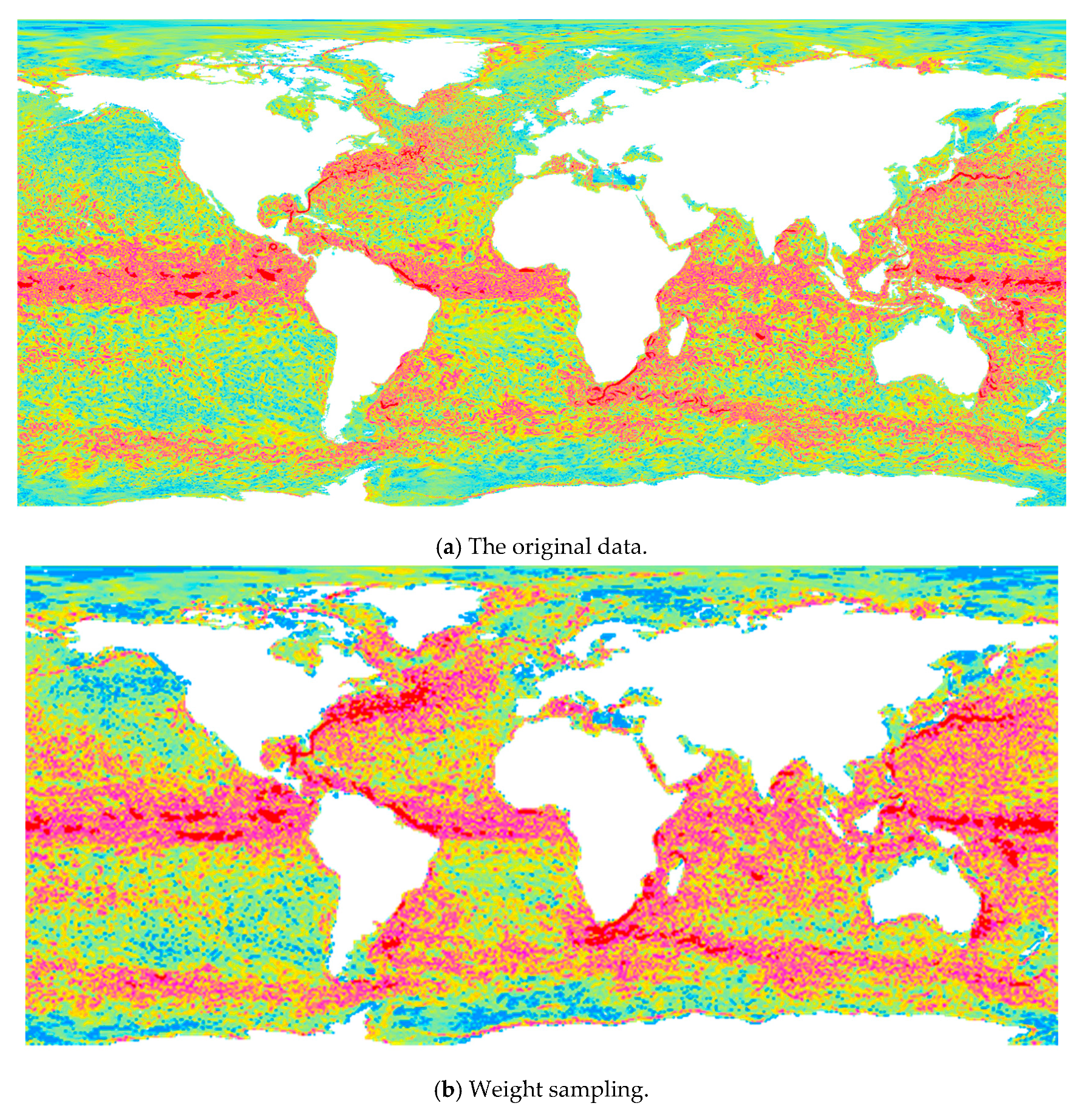
4. Integrated Mapping of Ocean Flow Fields

The weight analysis is helpful for capturing the characteristics of flow fields in detail when visualizing them. Multi-scale representation can meet the cognitive needs of users at different scales. Observing the data through the scale axis can deepen the visual perception, allow us to grasp the nature of the data, and help users to study the distribution, characteristics, and laws of flow fields at different scales. Creating an effective multi-scale visualization of ocean flow fields requires key scales determined by map load as well as point weights, which identify the most important data points for inclusion in the visualization [33].

In order to verify the validity of this analysis technique, this paper takes test data from the Kuroshio region and selects two verification regions. The first verification region is located to the west of the Cape of Good Hope in Africa, and the second verification region is located on the equator in the Pacific Ocean. The data are NetCDF(network Common Data Form) data provided by the North Sea Bureau of the Ministry of Natural Resources of China, and are numerical simulation forecast data.

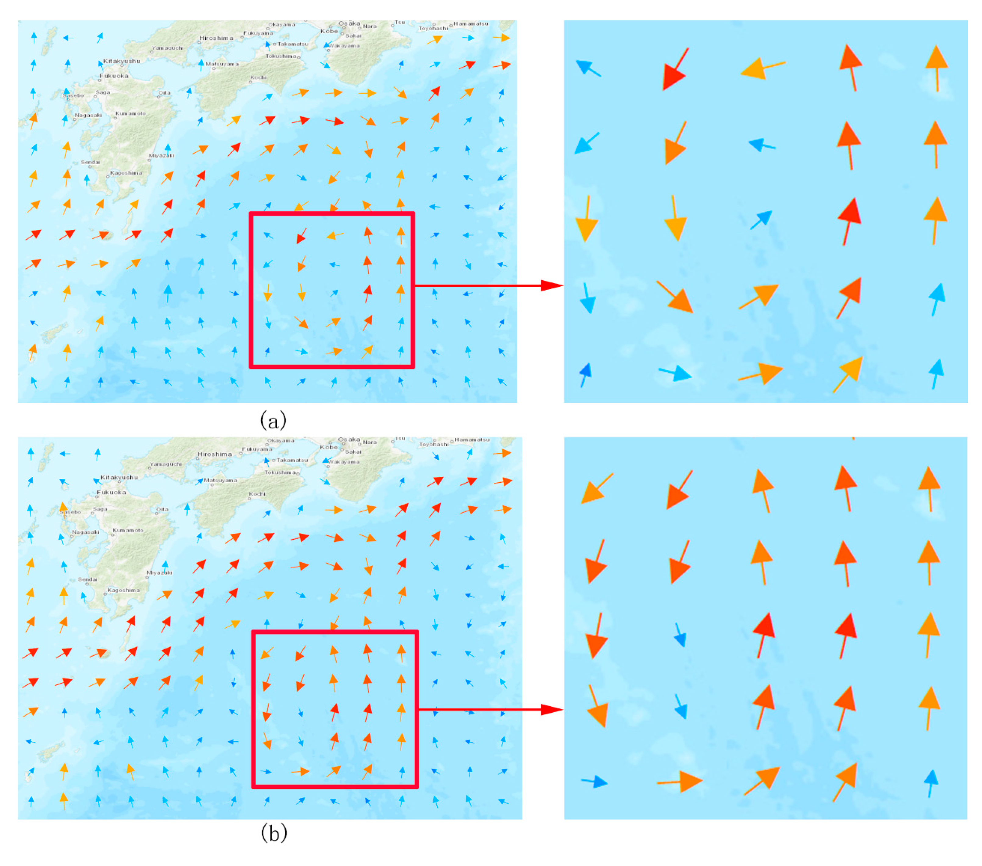
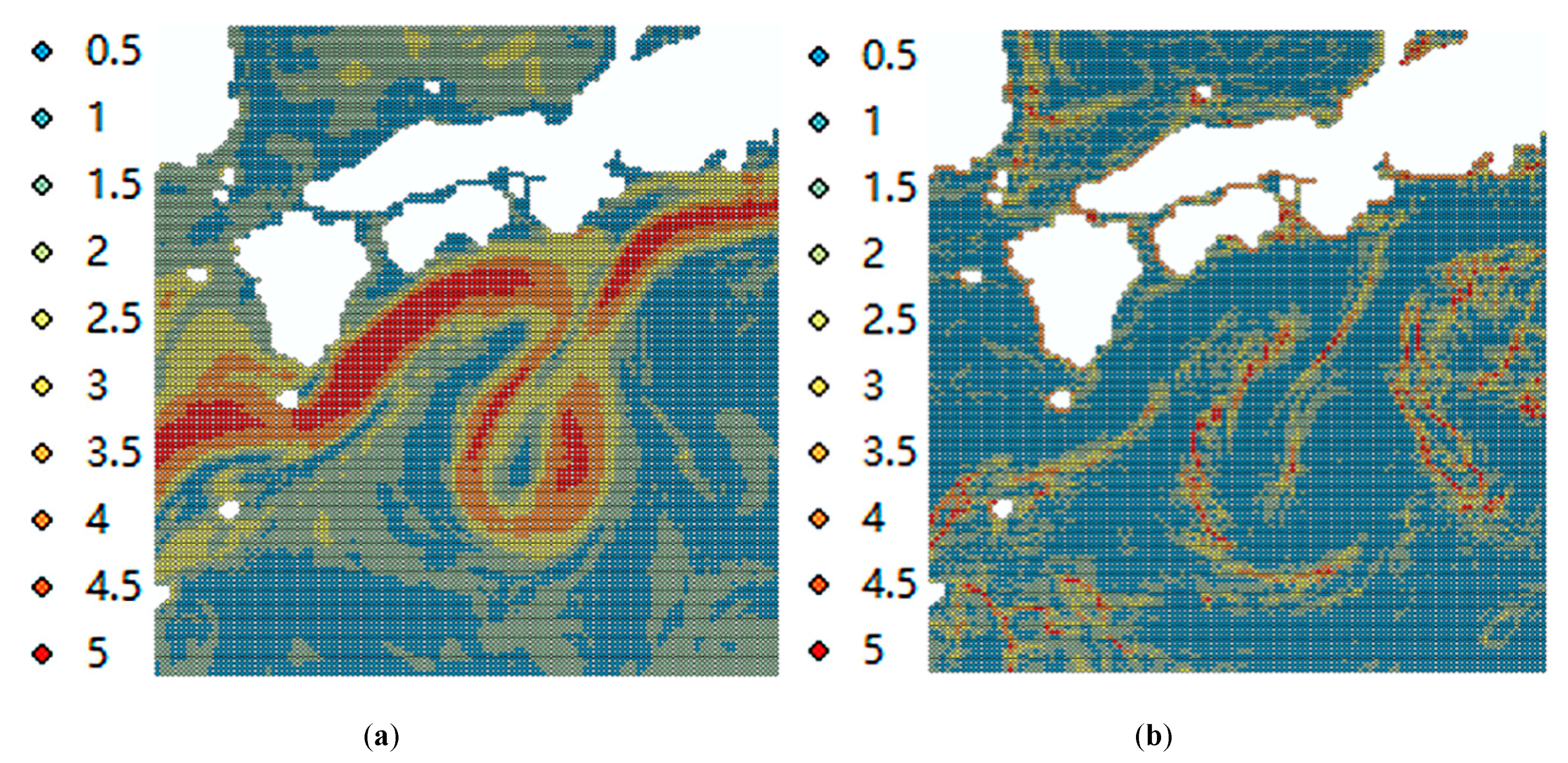
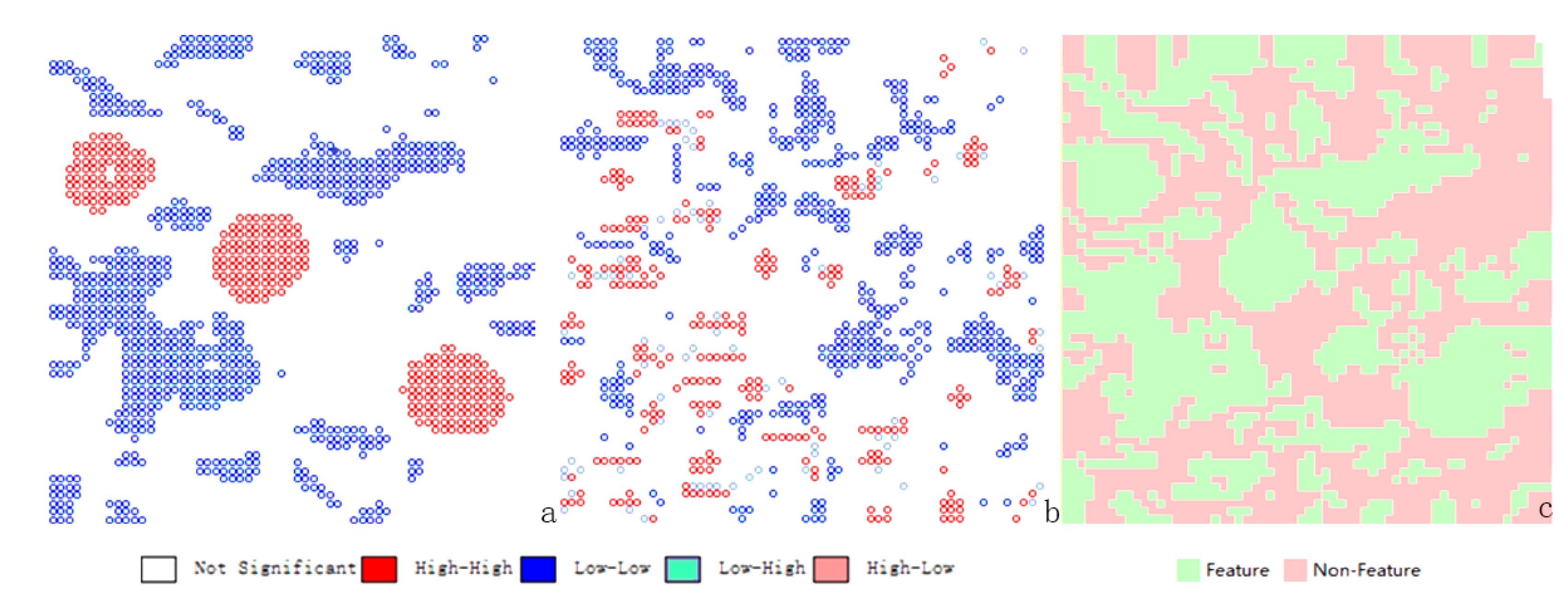
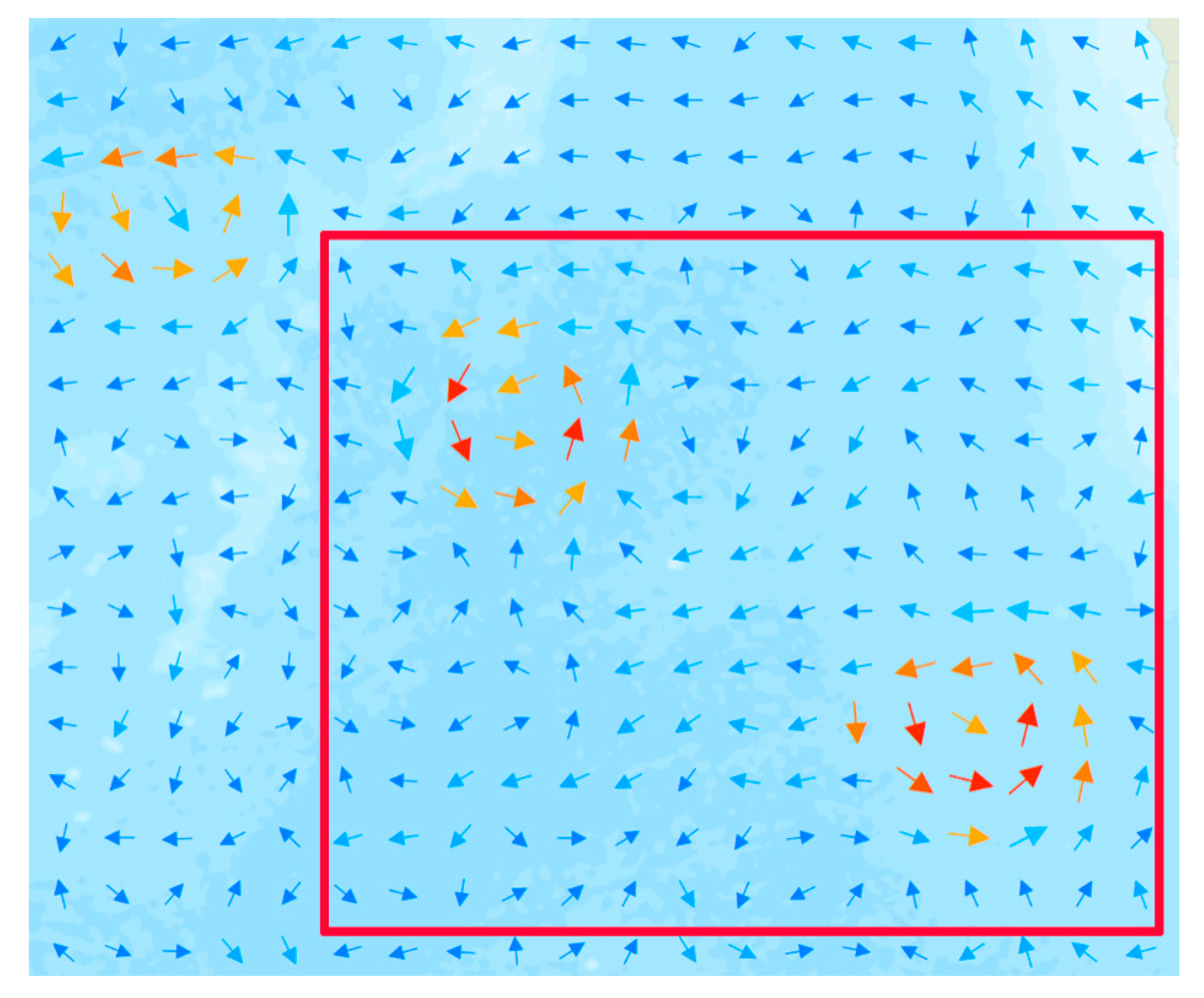
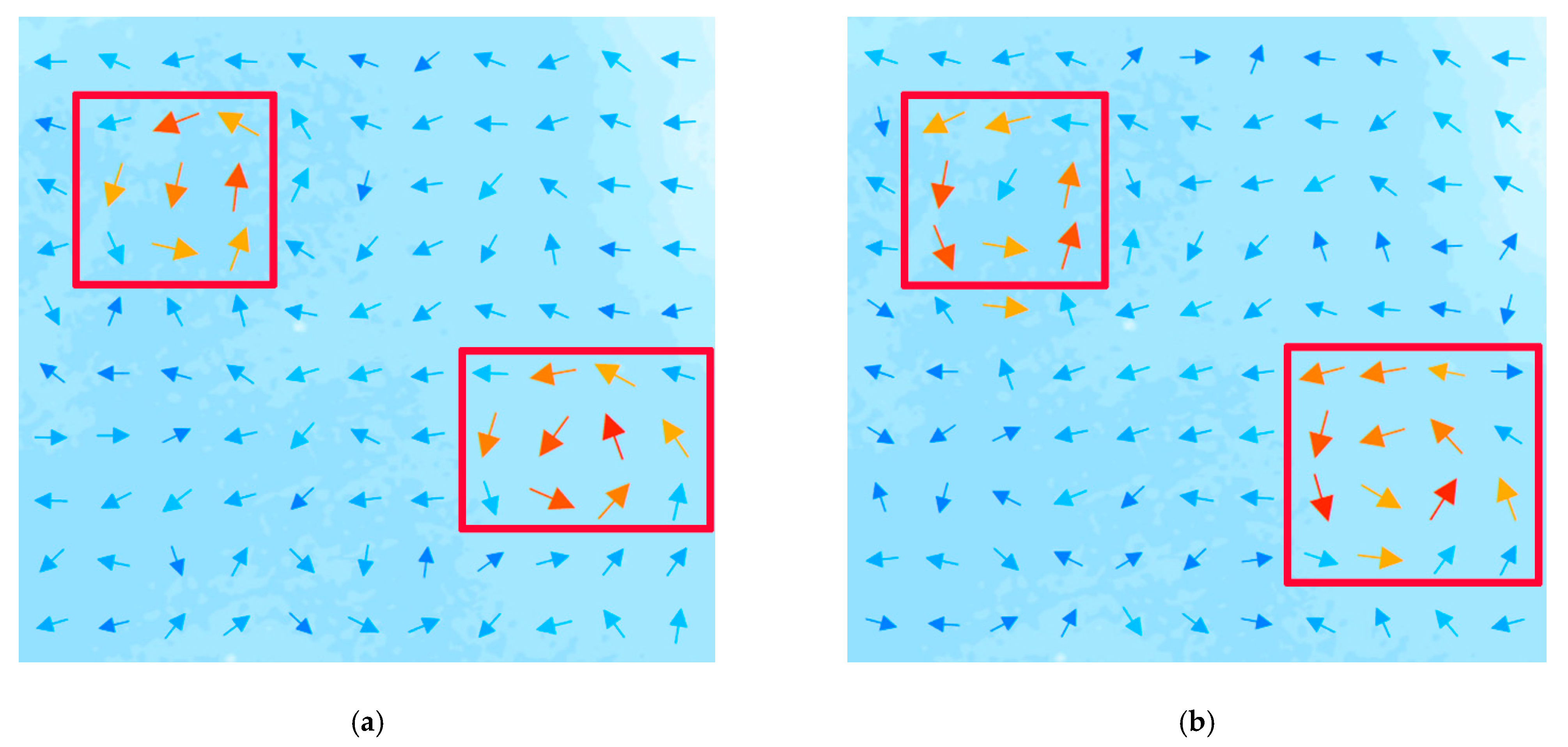
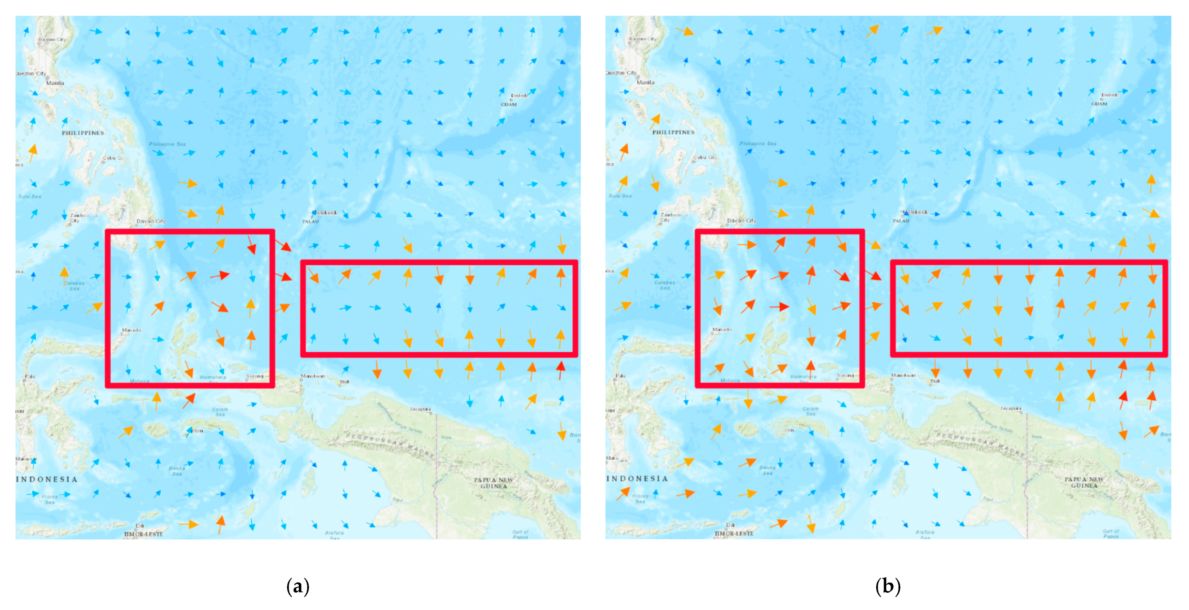
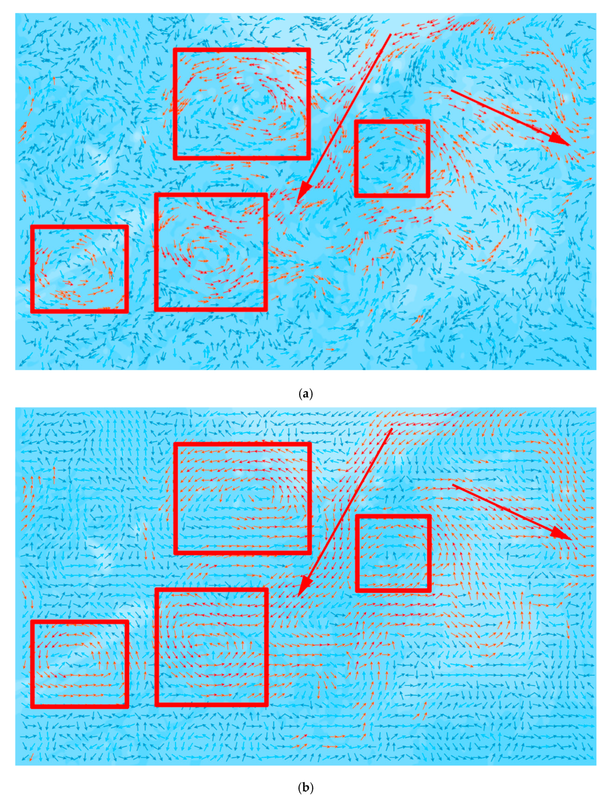
4.1. Integrated Mapping of Test Region

Integrated mappings based on the equidistant sampling method and the weight sampling method proposed in this paper are constructed at the same scale with the same thinning intervals. These maps are shown in Figure 6.

As can be seen from these maps, the weight sampling method shows some key characteristics of the Kuroshio current quite clearly, while they are somewhat less conspicuous on the map generated using the equidistant sampling method. The width of the Kuroshio, in reality, is wider than what is shown by the equidistant sampling method. This shows that the weight sampling method does a better job of preserving the flow field feature data than the equidistant sampling method.

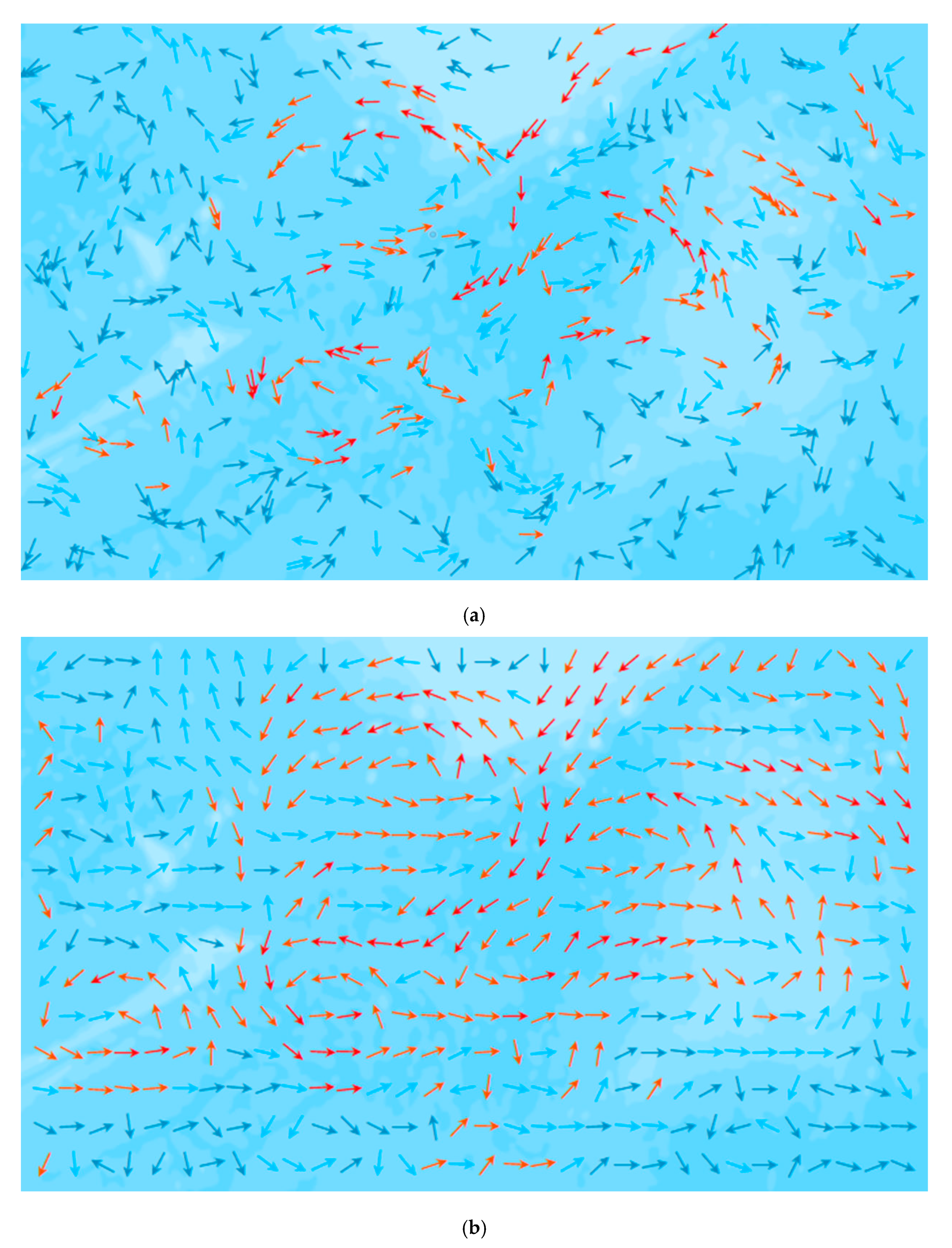
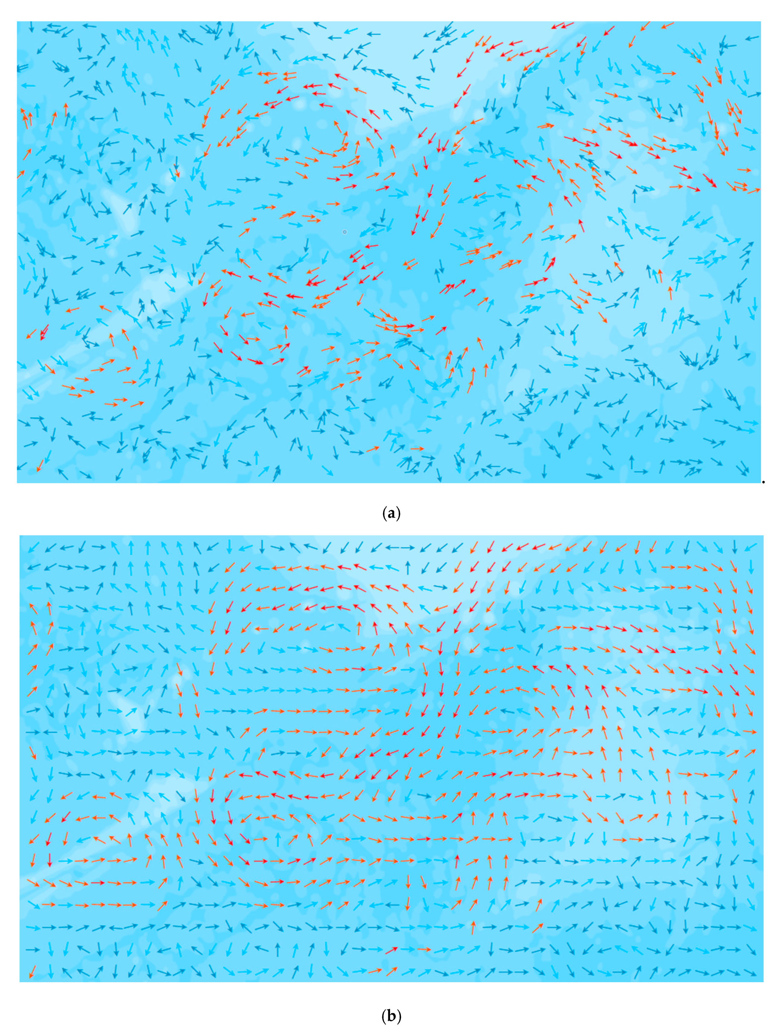
4.2. Integrated Mapping of Verification Region

The flow speed autocorrelation analysis and the direction change rates of flow autocorrelation analysis are carried out on data from the western area of the Cape of Good Hope (0~14.75 E, 23 S~37.75 S). The results are shown in Figure 7.

The weights are calculated according to rough set theory and evidence theory. The attribute weights are shown in

Table 4. African region attributed weight combination.

C	C1	C2	C3	C4
${\mathrm{W}}_{\mathrm{j}}^{\left(\mathrm{DS}\right)}$	0.29	0.19	0.34	0.18

.

After calculating the weights, calculated key scales are used to sample the data for a step size of three, as shown in Figure 8.

According to Figure 7 and Figure 8, there are three high speed vortices. The area inside the red frame in Figure 7 was selected, and both equidistant sampling and weight sampling were performed using calculated key scales at a step size of four, as shown in Figure 9.

In Figure 9, two high-speed vortices within the red square are compared, and it can be seen that the vortices shown in the weight sampling map are more balanced than those shown in the equidistant sampling method map. In addition, the range remains better.

The data from the Pacific Ocean equatorial region is processed in the same way (119.1 E~147.9 E, 8.2 S~17.8 N), and the results are shown in Figure 10.

Weights are calculated using the same method, and the results are shown in

Table 5. The equator of Pacific Ocean attribute weight combination.

C	C1	C2	C3	C4
${\mathrm{W}}_{\mathrm{j}}^{\left(\mathrm{DS}\right)}$	0.42	0.18	0.18	0.22

.

Representations of this portion of the equatorial current region are constructed according to these weights and the calculated key scales, and they are shown in Figure 11.

It can be seen in Figure 11 that equal sampling misses many feature points in the two red-bordered regions, while the weight sampling method retains more of these feature points.

Figure 9 and Figure 11 each represent data from regions that differ significantly from the Kuroshio test region, and the weight-sampling method retains key flow field features effectively in both cases. This indicates that using feature extraction, autocorrelation analysis, and classification analysis to determine weights for the purpose of data point sampling is indeed useful for feature preservation.

This paper selects the flow field data whose longitudes are from 11 E to 30 E and whose latitudes are from 44 S to 35 S, to further verify the effect and superiority of this method for feature retention. There are four main irregular vortices and two high-speed currents in this data. In view of the above experiments, it is verified that the method of this paper can retain features better than equal sampling, so stratified sampling is selected for comparison with the method in this paper. The criterion of stratified sampling is made according to whether it is a feature area. The sampling step size is in accordance with steps 3, 5 and 7, and the results are shown in Figure 12, Figure 13 and Figure 14.

Figure 12, Figure 13 and Figure 14 are the results of the two methods after increasing the sampling step size according to the scale change. When the step size is three, both methods retain features well. When the step size is five, weight sampling has more reserved feature points than stratified sampling, which makes feature reservation more regular. When the step size is seven, the features are almost invisible in stratified sampling, while the features of weight sampling are still clear, and the shape remains good. This shows that, compared with the stratified sampling method, weight sampling can retain and highlight the characteristics in the case of multi-scale expression with a smaller scale and a larger thinning step, which is more suitable for the thinning work in the case of multi-scale expression.

Finally, the effect of this method on global scale visualization is verified. In this scale, users are generally interested in the world’s ocean current, which is easy to identify on the map due to its fast speed and large area, and the fact that it is also a research hotspot. The direct visualization of global flow field data will cause serious symbol compression, so it requires a very long step sampling work. However, a long step will cause the loss of feature points of world ocean currents. The results are shown in Figure 15 using the weight sampling method for global data.

In Figure 15a is the global original resolution image, and in Figure 15b is the result of the weight sampling method. It can be seen from Figure 15 that the result of the weight method exaggerates the world ocean current compared with the original data, which can better solve the feature point loss of world ocean current caused by too large a step size.

5. Conclusions

In order to construct improved multi-scale representations of ocean flow fields, this paper proposed a weight-based method for sampling data points. First, autocorrelation analyses and classification analyses were carried out on two factors: flow speed and rates of direction change. Based on these analyses, the weights of data points were assigned according to the classification area where the data points were located. Next, these four factors were taken as four conditional attributes of the feature region, and rough set theory was used to calculate the support degree of each factor to the feature region. Then, evidence theory was used to combine these different attributes into a single weight for each data point. Finally, points were selected on the basis of weight in order to construct a multi-scale representation of ocean flow fields, which retained and visualized the key features of the flow field effectively. In this paper, experiments were carried out in four regions. The global flow field and different methods were used for comparison. The results show that the method is reliable in feature extraction work and retaining more features in multi-scale sampling.

References

1. Cai, Z.H. Rarefying and Representation of Flow Fields. Ph.D. Thesis, Capital Normal University, Beijing, China, 2013. [Google Scholar]
2. Wang, L.; Cheng, Y.; Hong, L.; Liu, X. A Novel Algorithm for Ocean Wave Direction Inversion from X-band Radar Images Based on Optical Flow Method. Acta Oceanol. Sin. 2018, 37, 88–93. [Google Scholar] [CrossRef]
3. Post, F.H.; de Leeuw, W.C.; Sadarjoen, I.A.; Reinders, F.; Van Walsum, T. Global, Geometric, and Feature-based Techniques for Vector Field Visualization. Future Gener. Comput. Syst. 1999, 15, 87–98. [Google Scholar] [CrossRef] [Green Version]
4. Fang, Y.; Ai, B.; Fang, J.; Xin, W.; Zhao, X.; Lv, G. Multi-Scale Flow Field Mapping Method Based on Real-Time Feature Streamlines. ISPRS Int. J. Geo-Inf. 2019, 8, 335. [Google Scholar] [CrossRef] [Green Version]
5. Leeuw, W.D.; Liere R, V. Visualization of Global Flow Structures Using Multiple Levels of Topology. In Data Visualization; Springer: Vienna, Austria, 1999. [Google Scholar]
6. Tricoche, X.; Wischgoll, T.; Scheuermann, G.; Hagen, H. Topology tracking for the visualization of time-dependent two-dimensional flows. Comput. Graph. 2002, 26, 249–257. [Google Scholar] [CrossRef] [Green Version]
7. Roth, M.; Peikert, R. Spatial and Temporal Variability of The Iberian Peninsula Coastal Low-level jet. Int. J. Climatol. 2018, 38, 1605–1622. [Google Scholar] [CrossRef]
8. Jiang, M.; Machiraju, R.; Thompson, D. A Novel Approach to Vortex Core Region Detection. Data Vis. Eurograph. Assoc. 2002, 17, 12–16. [Google Scholar] [CrossRef]
9. Tricoche, X.; Garth, C.; Scheuermann, G. Fast and Robust Extraction of Separation Line Features. IEEE Trans. Inf. Technol. Biomed. A Publ. IEEE Eng. Med. Biol. Soc. 2006, 14, 1291–1297. [Google Scholar] [CrossRef]
10. Weinkauf, T.; Theisel, H.; Hege, H.C.; Seidel, H.P. Boundary Switch Connectors for Topological Visualization of Complex 3D vector Fields. In Proceedings of the Data Visualization, Konstanz, Germany, 19–21 May 2004; pp. 183–192. [Google Scholar]
11. Theisel, H.; Weinkauf, T.; Hege, H.C.; Seidel, H.P. Stream Line and Path Line Oriented Topology for 2D Time-Dependent Vector Fields. In Proceedings of the IEEE Visualization, Austin, TX, USA, 10–15 October 2004; pp. 321–328. [Google Scholar]
12. Theisel, H.; Weinkauf, T.; Hege, H.C.; Seidel, H.P. Grid-independent detection of closed stream lines in 2D vector fields. In Proceedings of the Vision, Modeling and Visualization, Stanford, CA, USA, 16–18 November 2004. [Google Scholar]
13. Guenther, R.; Miklasz, K.; Carrington, E.; Martone, P.T. Macroalgal spore dysfunction: Ocean acidification delays and weakens adhesion. J. Phycol. 2017, 54, 153–158. [Google Scholar] [CrossRef]
14. Williams, S.; Petersen, M.; Bremer, P.T.; Hecht, M.; Pascucci, V.; Ahrens, J.; Hlawitschka, M.; Hamann, B. Adaptive Extraction and Quantification of Geophysical Vortices. IEEE Trans. Vis. Comput. Graph. 2011, 17, 2088–2095. [Google Scholar] [CrossRef] [Green Version]
15. Koehler, C.; Wischgoll, T.; Dong, H.; Gaston, Z. Vortex Visualization in Ultra Low Reynolds Number Insect Flight. IEEE Trans. Vis. Comput. Graph. 2011, 17, 2071–2079. [Google Scholar] [CrossRef]
16. Sadlo, F.; Peikert, R. Efficient Visualization of Lagrangian Coherent Structures by Filtered AMR Ridge Extraction. IEEE Trans. Vis. Comput. Graph. 2007, 13, 1456–1463. [Google Scholar] [CrossRef] [Green Version]
17. Lipinski, D.; Mohseni, K. A ridge tracking algorithm and error estimate for efficient computation of Lagrangian coherent structures. Chaos Interdiscip. J. Nonlinear Sci. 2010. [Google Scholar] [CrossRef] [PubMed]
18. Doleisch, H.; Gasser, M.; Hauser, H. Interactive feature specification for focus+context visualization of complex simulation data. VisSym 2003, 3, 239248. [Google Scholar]
19. Xu, H.; Li, S. Intelligent Flow Feature Extraction and Multi-Resolution Visualization. J. Comput. Aided Des. Comput. Graph. 2008, 20, 571–576. [Google Scholar]
20. Enya, S.; Liang, Z.; Huaxun, X.; Sikun, L. Fuzzy-based Interactive Feature Description and Extraction of 3D Flows. J. Image Graph. 2011, 16, 1121–1126. [Google Scholar]
21. Chen, J.; Yang, S.; Li, H.; Zhang, B.; Lv, J. Research on Geographical Environment Unit Division Based on the Method of Natural Breaks (Jenks). ISPRS Int. Arch. Photogramm. Remote Sens. Spat. Inf. Sci. 2013, XL-4/W3, 47–50. [Google Scholar] [CrossRef] [Green Version]
22. Ming, L. Research and Implementation of Visualization Method for Marine Environment Early Warning Data; Capital Normal University: Beijing, China, 2014. [Google Scholar]
23. Bin, X. Simulation Analysis of the Influence of Spatial Weight Matrix on Moran’s I; Nanjing Normal University: Nanjing, China, 2007. [Google Scholar]
24. Basir, O.; Yuan, X. Engine fault diagnosis based on multi-sensor information fusion using Dempster–Shafer evidence theory. Inf. Fusion 2007, 8, 379–386. [Google Scholar] [CrossRef]
25. Sun, L. Improved Method of Attribute Weight Based on Rough Theory. Comput. Eng. Appl. 2014, 50, 43–45. [Google Scholar] [CrossRef]
26. Thangavel, K.; Pethalakshmi, A. Dimensionality reduction based on rough set theory: A review. Appl. Soft Comput. 2009, 9, 1–12. [Google Scholar] [CrossRef]
27. Pawlak, Z. Rough set. Int. J. Comput. Inf. Sci. 1982, 11, 1655–1666. [Google Scholar] [CrossRef]
28. Ahn, B.S.; Cho, S.S.; Kim, C.Y. The integrated methodology of rough set theory and artificial neural network for business failure prediction. Expert Syst. Appl. Expert Syst. Appl. 2000, 18, 65–74. [Google Scholar] [CrossRef]
29. Suo, Y.Q.; Ma, L.; Tan, W. A Modified Heuristic Algorithm of Attribute Reduction in Rough Set. J. Xi’an Univ. Post Telecommun. 2009, 14, 116–120. [Google Scholar] [CrossRef]
30. Li, L.; Cao, L.; Liu, B.; Li, H.; Zhou, Y. The Method of Attribute Weight Distribution in Multi-attribute System. Trans. China Electrotech. Soc. 2015, S1, 422–427. [Google Scholar]
31. Liu, H.; Qian, Y. Evaluation of Simulation Credibility Based on Rough Set and Gray Correlation Analysis. J. Syst. Simul. 2018, 30, 459–464. [Google Scholar] [CrossRef]
32. Wang, H.; Yao, B.; Hu, H. Weight determination method based on rough set theory. Comput. Eng. Appl. 2003, 39, 20–21. [Google Scholar]
33. Ai, B.; Liu, Y.; Wang, Z.; Sun, D. Evaluation of multi-scale representation of ocean flow fields using the Euler method based on map load. J. Spat. Sci. 2019. [Google Scholar] [CrossRef]
Figure 1. The flow chart of multi-scale representation of ocean flow fields based on feature analysis.
Ijgi 09 00307 g001
Figure 2. Results of autocorrelation analysis of Kuroshio’s speed.
Ijgi 09 00307 g002
Figure 3. Diagram of variation rate of direction.
Ijgi 09 00307 g003
Figure 4. Autocorrelation analysis of Kuroshio direction change rates of flow.
Ijgi 09 00307 g004
Figure 5. Kuroshio data classification analysis weight distribution. (a) is the classification analysis results of flow speed, according to Equation (11), it is divided into 10 regions; (b) is the classification analysis results of direction change rates of flow, according to Equation (12), it is divided into 10 regions.
Ijgi 09 00307 g005
Figure 6. Comparison of Kuroshio in two sampling methods: (a) equal sampling; (b) weight sampling.
Ijgi 09 00307 g006
Figure 7. African data analysis(Resolution = 0.25). (a) Flow speed autocorrelation analysis, (b) Direction change rates of flow autocorrelation analysis, (c) Feature region and non-feature region, (a,b) are the results of autocorrelation analysis, which are divided into five types of data points: not significant, high-high, low-low, low-high, high-low. (c) is the classification map of feature regions and non-feature regions, which are used for the decision attribute of rough set theory.
Ijgi 09 00307 g007
Figure 8. Weight sampling of the African region (step size = 3).
Ijgi 09 00307 g008
Figure 9. Comparison of African region in two sampling methods (step size = 4). (a) is the result of equal sampling, (b) is the result of Weight sampling, and feature points are in the red square.
Ijgi 09 00307 g009
Figure 10. The equator of Pacific Ocean data analysis(Resolution = 0.1). (a) Flow speed autocorrelation analysis. (b) Direction change rates of flow autocorrelation analysis. (c) Feature region and non-feature region. (a,b) are the results of autocorrelation analysis, which are divided into five types of data points: not significant, high-high, low-low, low-high, high-low. (c) is the classification map of feature regions and non-feature regions, which are used for the decision attribute of rough set theory.
Ijgi 09 00307 g010
Figure 11. Comparison of equator of Pacific Ocean in two sampling methods. (a) is the result of equal sampling, (b) is the result of Weight sampling, and feature points are in the red square.
Ijgi 09 00307 g011
Figure 12. Comparison of equator of region in two sampling methods (step = 3; scale: 1:8,000,000). (a) is the result of Stratified sampling., (b) is the result of Weight sampling, and feature points are in the red square.
Ijgi 09 00307 g012
Figure 13. Comparison of equator of region in two sampling methods (step = 5; scale: 1:10,000,000). (a) is the result of Stratified sampling., (b) is the result of Weight sampling, and feature points are in the red square.
Ijgi 09 00307 g013
Figure 14. Comparison of equator of region in two sampling methods (step=5; scale: 1:15,000,000). (a) is the result of Stratified sampling., (b) is the result of Weight sampling, and feature points are in the red square.
Ijgi 09 00307 g014
Figure 15. The original data and the weight sampling (step = 8). (a,b) are the global original resolution image and the result of the weight sampling method. The color changes from red to blue according to the speed. The region in red represents the highest speed classification and the region in blue represents the lowest speed classification.
Ijgi 09 00307 g015