1. Introduction
The Earth is an unsteady planet that constantly changes due to the influence of diverse dynamic processes that are happening in the Earth’s interior, at its surface, and in its atmosphere. Triggers for these dynamic processes are major internal and external forces that act upon our planet. Internal or endogenous forces act upon our planet from within, starting at the core, over the mantle, and up to the crust (oceanic and continental). Internal processes are constantly deforming Earth’s surface due to the increase of stress with depth, resulting from gravitational forces beneath and at the Earth’s surface [
1]. External or exogenous forces, on the other hand, act upon Earth’s body from the outside. Weathering, erosion, and other natural phenomenon effects model the Earth’s physical surface. However, deformations of the Earth’s body are also induced by the attraction of the Moon and the Sun [
2]. Owing to dynamic processes in its interior, atmosphere, and ocean, many areas of the Earth’s surface are liable to natural disasters such as earthquakes, volcano eruptions, floods, tsunamis, global warning, and others [
3]. Scientists are putting great effort towards better understanding the changes Earth undergoes, where one of the main objectives is to anticipate natural hazards. Inducements for some of these natural hazards have their roots in the motions of Earth’s tectonic plates. The dynamics and evolution of the solid Earth, among others, cause movements and deformations of the tectonic plates [
4]. Modeling and processing observations of large data sets are often required to better understand these processes.
Features of geodesy, as a science which deals with measurement and mapping of the Earth’s surface, are still fundamental today. Bearing this in mind, fundamental features of geodesy have to be extended with the knowledge that Earth’s gravity field determines its shape. The modern understanding of geodesy has its basis expanded for procedures that deal with precise measurements and determination of the Earth’s geometric shape, its orientation in space, and its gravity field, as well as its evolution in time.
Satellite-based measuring techniques continually undergo changes and advancements that have a significant impact in the field of geodesy. As a consequence, increasingly accurate reference frames and kinematic models are defined. Due to new and more accurate realizations of reference frames, the need to coordinate transformations between them is increasing every day. The fact that points on the Earth’s surface are not stationary but are a function of time due to the motion of tectonic plates increases the need for faster and simpler temporal coordinate transformation. We came to the conclusion that the scientists and experts dealing with the everyday need for simpler and faster temporal coordinate transformation would largely benefit from one such unique application. Before taking any further steps, research regarding similar transformation tools was carried out. The available online tools (see [
5,
6,
7], etc.) were tested to check the possibility of point velocity calculation and, eventually, velocity transformation simultaneous with coordinate transformation. The results of that testing showed that the existing available web and similar tools have only features of basic coordinate transformation, without the possibility of further velocity computation and transformation. With regard to that research, development of the TranSAB standalone desktop application was initiated.
The TranSAB standalone desktop application is the product of our desire and vision to connect different scientific fields into one compatible, functional, and sustainable system. The TranSAB application enables coordinate transformation between different realizations of the International Terrestrial Reference System (ITRS) and European Terrestrial Reference System 1989 (ETRS89) published up till now. However, what makes this application original is the possibility to compute station velocities due to annual coordinate shifts caused by plate tectonics. Station velocities are obtained from appropriate kinematic models of the Eurasian tectonic plate and original kinematic models of the Adriatic microplate (which is part of the Eurasian plate and deployed by our own research [
8,
9,
10]). In addition to their calculations, the user has the option to transform velocities in an a priori defined reference frame.
2. The Terrestrial Reference Frame as a Product of the “Three Pillars” of Geodesy
The Earth, its environment, and other celestial bodies do not have absolute positions in the universe; they move, rotate, and are subject to changes. The tasks of geodesy, geophysics, and astronomy are to foresee (determine) their kinematics and dynamics [
11]. In order to predict those behaviors, it is of great necessity to have available data sets (positions and velocities) uniformly distributed across the surface of the Earth. As positions and velocities obtained by geodetic measurements are not direct observations, but estimated quantities, this raises the need for a terrestrial reference in which positions and velocities can be expressed [
12]. According to that need, the Terrestrial Reference Frame (TRF) becomes a terrestrial reference. A TRF is a set of physical points with precisely determined coordinates in a discrete coordinate system [
13] and, as such, it represents the realization of the theoretically defined Terrestrial Reference System (TRS) [
14].
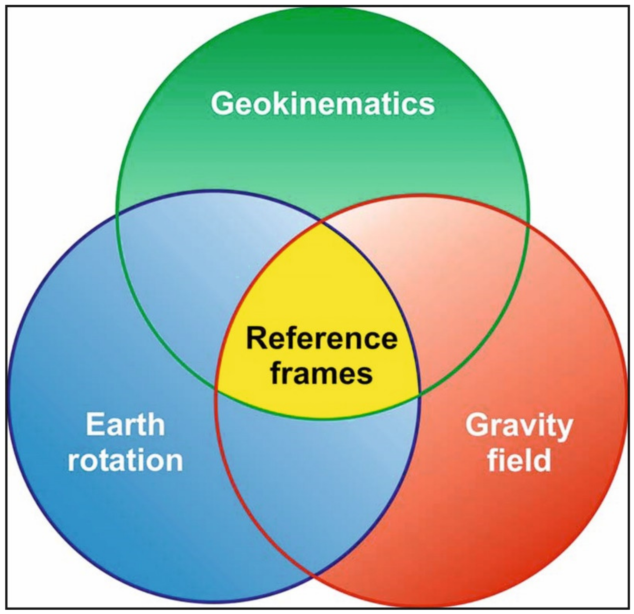
The “three pillars” of geodesy, as shown in
Figure 1, refer to Earth’s time-dependent geometric shape, time-dependent gravitational field, and rotation [
15]. They represent a conceptual and observational basis for the reference frames essential and inevitable for observation of the Earth. These three pillars are mutually attached and intertwine as they provide divergent observations related to the same Earth processes [
3].
3. Geodynamical Phenomena—Plate Tectonics
According to geology, a plate is a massive and rigid creation of solid rock, whereas the word tectonic is derived from the Greek language and it refers to the word to build. The theory of plate tectonics originated at the end of the 16th century when Sir Francis Bacon noticed a matching shape of coastal lines of the American and African continents in his observations [
16]. Following that theory, it can be stated that Earth’s crust consists of 14–16 major lithospheric plates that float on the viscous hot asthenosphere [
17]. For the last 30 years, space geodetic measurements have been used to determine plate tectonic movements [
18]. Data obtained by space geodetic measurements have been used to test the hypothesis that plate motions are stable. Thus, it is considered whether the average observations of rates and displacements of plate tectonics obtained over a short period (a few years) are similar to average rates and displacements of plate tectonics obtained from systematic estimations of marine magnetic anomalies (long period, over a million years) [
19]. Quantifying plate tectonic motion is significant for understanding the inner structure and behavior of tectonic plates, which includes the relations these processes have with earthquakes and volcanic activities. As mentioned above, data obtained by space geodesy measurements enable assessments of plate motions at the sub-centimeter level each year [
20].
The velocities of points on the physical surface of the Earth are caused by plate movements and can be described by kinematic models of plate tectonic motions. Kinematic models can be determined by two independent data sets (or a combination of them) or by satellite geodesy data [
8]. According to Becker and Facenna [
21], plate motion models can be divided into two main groups: absolute kinematic models, defined in the absolute reference frame, and relative kinematic models, defined in the reference frame of plate motion relative to another. For plate kinematics and dynamic analysis needs, two absolute reference frames have been applied [
22]: the hotspot reference frame (HSRF), based on the assumption that discrete hotspots are relative to the mesosphere and mutually, and the no-net-rotation (NNR) frame, based on the assumption that the lithosphere and the asthenosphere are inextricably linked to one another. Current plate motion models are defined by the NNR condition, or, in other words, rotation of the reference system is zero with respect to the Earth’s lithosphere. That means that the reference system has no constraints with regard to the lithosphere movements [
8]. Furthermore, NNR can mathematically be expressed as a Tisserand condition. The Tisserand condition states that the sum of the total angular momentum of the whole Earth (all Earth’s plates) is zero, and can be expressed as [
23]
In Equation (1), is the summation of the total angular momentum of the Earth’s lithosphere, is the velocity vector of its corresponding position vector (), D is the whole Earth’s lithosphere surface, and dm is a unit mass of the Earth.
The tectonic plate included in a certain kinematic model is determined by six parameters [
24]. Three of these parameters are related to the Euler pole: geodetic latitude,
ϕ (
°); geodetic longitude,
λ (
°); and angular velocity,
Ω (
°/
Myr). The other three components are related to the Euler rotation vector (
) and represent the angular rotation vector (
) in a Cartesian geocentric frame (usually in units of
rad/Myr). The link between the Euler rotation vector and Euler pole is given by Equation (2) [
24]:
where the reverse relation is given in Equation (3):
At a location defined by coordinates (
XT, YT, ZT) of a point
T at the Earth’s surface, the velocities for a Euler rotation vector are given as [
24]
In Equation (4), VX/ΔT, VY/ΔT, and VZ/ΔT are in units of mm/year.
4. European Reference Frame (EUREF) Official Transformations Between Different Reference Frames
The European Terrestrial Reference System 1989 (ETRS89) was adopted in 1990 in Firenze, Italy, following EUREF Resolution 1 [
25]. This resolution states that ETRS89 is coincident with the ITRS89 at the epoch 1989.0 and is fixed to the stable part of the Eurasian plate [
26]. Plate tectonics in the global ITRS causes European station coordinates to shift; hence, fixing ETRS89 to the stable part of the Eurasian plate at the initial epoch 1989.0 enables minimal time dependencies between the coordinates of stations located in the stable part of Europe [
27].
EUREF Technical Note (TN) (1) [
28] summarized and replaced EUREF Memos (8) published between 1993 and 2011.
The general mathematical relation between two three-dimensional Cartesian coordinate systems (
X, Y, Z)
A and (
X, Y, Z)
B which enables coordinate and velocity transformations is given as [
29]
where
T = (
TX, TY, TZ)
T is the translation vector,
D is the scale factor, and
R is the rotation matrix. In Equation (5), the dotted parameters are time derivations of the transformation parameters (their rates). The rotation matrix
R contains Euler rotation angles and is given by Equation (6):
The relations between ETRS89 and ITRS, used for station (coordinates and velocities) transformations, are the outcome of the ETRS89 definition and are expressed as
where (
and (
are position and velocity couples for
yy realizations in ITRS and ETRS89. In Equation (7), translation vector
Tyyis utilized for origin offset, if there is one, between the different ITRF realizations. The rotation rate parameters
are three components—angular velocities of the Eurasian plate (Euler rotation angles) expressed in ITRFyy—and are listed in
Table 1 and Appendix A in Altamimi [
28].
Until the ETRF97 solution, which includes it, the Eurasia angular velocity in the corresponding ITRF solution was taken from kinematic models that were used in the NNR condition. They were the AMO2 model of Minster and Jordan [
30] and NNR-NUVEL1 and NNR-NUVEL1-A of Argus and Gordon [
31], based on the relative plate motion model of DeMets et al. [
32].
Beginning with the ITRF2000 realization, Eurasia angular velocities (including other plates) were estimated using ITRF velocity fields: ITRF2000, ITRF2005, ITRF2008, and ITRF2014 [
20,
33,
34,
35]. Using these procedures, ETRF2000 became the first realization of ETRS89 that evaluated angular velocities of the Eurasia tectonic plate using an ITRF velocity field [
36].
To express the EUREF Global Navigation Satellite System (GNSS) Network solution in ETRS89, proposed procedures to process GNSS data sets (observations) of a local (regional) EUREF network, referred to as a central epoch
tc, are composed of two steps. The first step is computing station coordinates in ITRS, followed by transforming into ETRS89 [
28].
Computation of GNSS data in ITRS at epoch
tc is explained in detail in EUREF TN-1 [
28]. Coordinates should be expressed at the central epoch
tc of the GNSS observations with respect to the initial epoch
t0, where applicable, by the expression
Users should bear in mind that if full compatibility with the ETRS89 definition is required, it is not recommended to propagate station coordinates from the central epoch
tc to any other epoch, based on any intraplate velocities, as mentioned in Altamimi [
28].
5. The TranSAB Application
The idea of binding different fields together was born by considering our affiliations to geodesy and geoinformatics. Furthermore, the fact that Python is one of the most popular programming languages today, as well as being widely used in geosciences, has led to its deeper study. Consequently, merging theoretical knowledge of Earth’s dynamic processes with Python resulted in the development of a computer application.
Python is a powerful interpreted, dynamic, object-orientated programing language. It was created in the early 1990s by Guido van Rossum at Centrum Wiskunde & Informatica (CWI) in the Netherlands. It is a multiplatform programing language, compatible with Mac OS X, Windows, Linux, Unix, and other operating systems. Furthermore, it is also open-source software. The properties mentioned above, in addition to its simple, easy to learn syntax, have made Python a very popular programming language today. A huge reason for choosing Python was its ease of learning, and although Python has some flaws (i.e., it is slower than its competitors, it has limitations with database access, and it is not very good for mobile development), those flaws were not crucial enough to abandon it, mainly because of Django. Django is a Python web framework, and for future TranSAB application development in the sense of web migration and the consequently expanding user range, Django and Python seemed to be great choices.
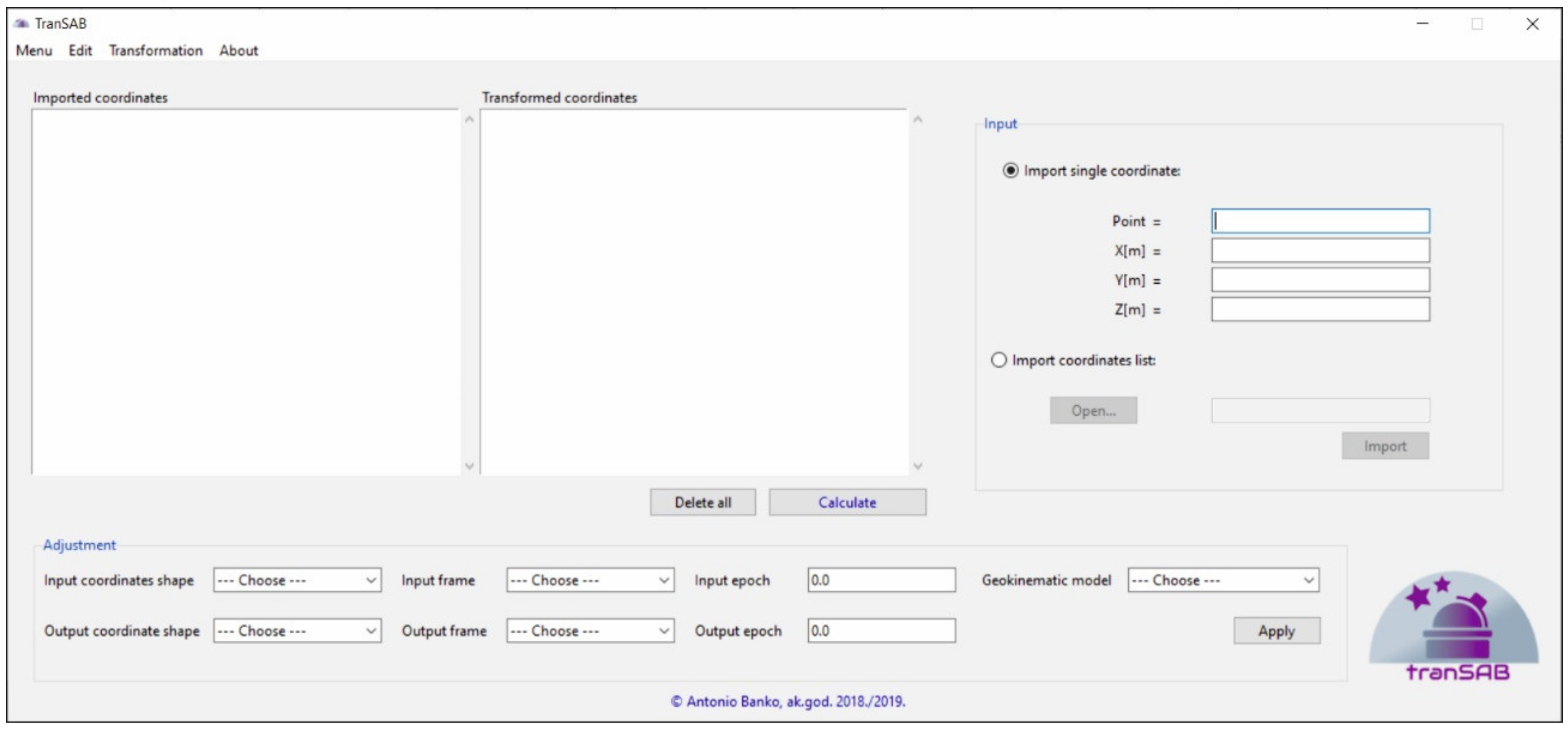
The application’s main scope is coordinate transformation between ITRS and ETRS89, that is, their realizations with the additional possibility of temporal coordinate transformation between them. The graphical user interface (GUI) of the TranSAB application is displayed in
Figure 2.
When transforming between realizations of the two systems, ITRS and ETRS89, the following transformations can be applied: TRF
yy ↔ ITRF
xx, ITRF
yy ↔ ETRF
yy, ITRF
yy ↔ ETRF
xx, and ETRF
yy ↔ ETRF
xx, where
yy and
xx are realizations of ITRS and ETRS89 (e.g., ITRF2000, ETRF2014, etc.). Thirteen ITRS solutions (ITRF88, 89, 90, 91, 92, 93, 94, 96, 97, 00, 05, 08, and 14) and eleven ETRS89 solutions (ETRF89, 90, 91, 92, 93, 94, 96, 97, 00, 05, and 14) have been published up till now.
Table 1 presents the European Petroleum Survey Group (EPSG) codes of ellipsoidal three-dimensional and Earth-centered, Earth-fixed (ECEF) coordinate systems (CS) of official ITRS realizations [
6].
Table 2 lists the EPSG codes of ellipsoidal three-dimensional and ECEF coordinate systems of official ETRS89 realizations [
6].
In addition to that, TranSAB has a temporal coordinate transformation feature where station velocities can be determined/imported with the use of two procedures: manual input of station velocities (m/yr.) or computation of station velocities from global NNR kinematics models of the Eurasia tectonic plate (m/yr.).
The global NNR kinematic models utilized in the TranSAB application are NNR-NUVEL-1 [
31], NNR-NUVEL-1A [
32], APKIM2000 [
37], ITRF2000 [
38], PB2002 [
39], APKIM2005 [
40], ITRF2005 [
34], MORVEL56 [
41], ITRF2008 [
35], MODEL-2008 [
8,
9], CRO-2014 [
10], CRODYN-2014 [
10], GEODYN-2014 [
10], and ITRF2014 [
20].
The EUREF online transformation service [
5] that allows coordinate transformation (position and velocity) between ITRS and ETRS89 realizations was used as a tool to validate the results obtained by TranSAB. The recommendations given by the EUREF Technical Working Group (TWG) in EUREF TN were followed, and transformation parameters from
Table 1 and Appendix A published in Altamimi were adopted [
28]. The general formula used to transform coordinates (position and velocity) between realizations of ITRS and ETRS89 is given by Equation (5), where, in the case of a different input epoch (central epoch
tc) with regard to the initial epoch
t0, it is mandatory to propagate parameters to the central epoch of observation using Equation (9). When transformation between two globally defined reference frames takes place (i.e., rotation between two global reference systems), the rotation matrix for the conventional IERS case (rotation from the to-frame to the from-frame) should apply.
It should be noted that the EUREF TWG does not recommend the use of ETRF2005 but rather the adoption of ETRF2000 as a conventional frame of the ETRS89 [
26].
Several internal TranSAB structural processes are inevitable for the work of the application itself. If ellipsoidal (φ, λ, h) or plane (E, N, h) coordinates are chosen as the input and/or output coordinate format, coordinate conversion will be the first and/or the last step of the application’s workflow. Plane coordinates (E, N, h) refer to the plane projection coordinates of transverse Mercator projection. Upon coordinate conversion, GRS80 ellipsoid is used as a mathematical model of the Earth’s body.
If, during transformation, velocity transformation is being carried out, then velocity transformation runs parallel with the coordinate transformation.
5.1. ITRFyy ↔ ITRFxx Transformation
Transformation (position and velocity, if needed) between any two ITRF solutions can be done by a one-step procedure by using the 14 transformation parameters adopted from Appendix A of EUREF TN-1 [
28] and the general formula given by Equation (5). It should be noted that the transformation parameters between any two realizations of ITRS can be easily derived from the above-mentioned appendix. It can be accomplished by determining the difference between the transformation parameters of the output and input reference frames. The parameters from Appendix A [
28] are provided at epoch
t0 = 2010.0; therefore, prior to transformation, the user should propagate the values at the central epoch of observation
tc using Equation (9).
5.2. ITRFyy ↔ ETRFyy Transformation
Position transformation and, if requested, velocity transformation between two corresponding frames of the ITRS and ETRS89 (e.g., ITRF2000 and ETRF2000) are achieved by applying Equations (7) and (8) in the case of velocity transformation. This type of transformation can be done by a one-step procedure by using the 14 transformation parameters. The transformation parameters can be found in
Table 1 in Altamimi [
28] and are given at the epoch
t0 = 1989.0. If transformation is requested at a different epoch, the parameters of transformation should be propagated at the central epoch of the observation by using Equation (9). The parameters are given for the ITRF to ETRF direction; if reverse transformation is called upon (ETRF to ITRF), the transformation parameters and rates are sign-changed to negative values.
5.3. ITRFyy ↔ ETRFxx Transformation
The position (and velocity) of station points can be transformed between different realizations of ITRS and ETRS89 by using the 14 transformation parameters and a two-step procedure. The first step implies transformation between ITRF
yy(
tc) and ITRF
xx(tc) or ETRF
yy(
tc) and ITRF
yy(
tc), depending on which one is the input frame. The second step is dealing with the transformation from ITRF
xx(
tc) to ETRF
xx(
tc) or, in the second case, from ITRF
yy(
tc) to ITRF
xx(tc). Details on how to transform in this case are mentioned in
Section 5.2 and
Section 5.3, respectively.
5.4. ETRFyy ↔ ETRFxx Transformation
This form of transformation is the most complex one. The procedure consists of two steps, where the second step is divided into two more steps. The first step pertains to the case of ETRF
yy(
tc) to ITRF
yy(
tc) transformation, where details can be found in
Section 5.2. In the second step, transformation from ITRF
yy(
tc) to ITRF
xx(tc) first needs to be applied; afterwards, in the last step, transformation from ITRF
xx(
tc) to ETRF
xx(
tc) is carried out. Directions for those operations are described in
Section 5.1 and
Section 5.2. The processing instructions mentioned in this subsection can be applied for both position transformation and velocity transformation cases.
5.5. Temporal Coordinate Transformation
If the user requires velocity transformation, temporal coordinate transformation is the last process of the TranSAB workflow. This transformation occurs due to shift of the point’s position. A general formula is presented in the following equation [
42]:
where
X(
t) is the position vector of the point in the reference frame expressed at epoch
t (
t is the output epoch).
X(
tc) is a position vector in the reference frame at the central epoch
tc of the observation.
V is a velocity vector in the corresponding reference frame.
X(
tc) and
V are obtained by the previously described transformation forms, and
t – tc is an epoch deduction.
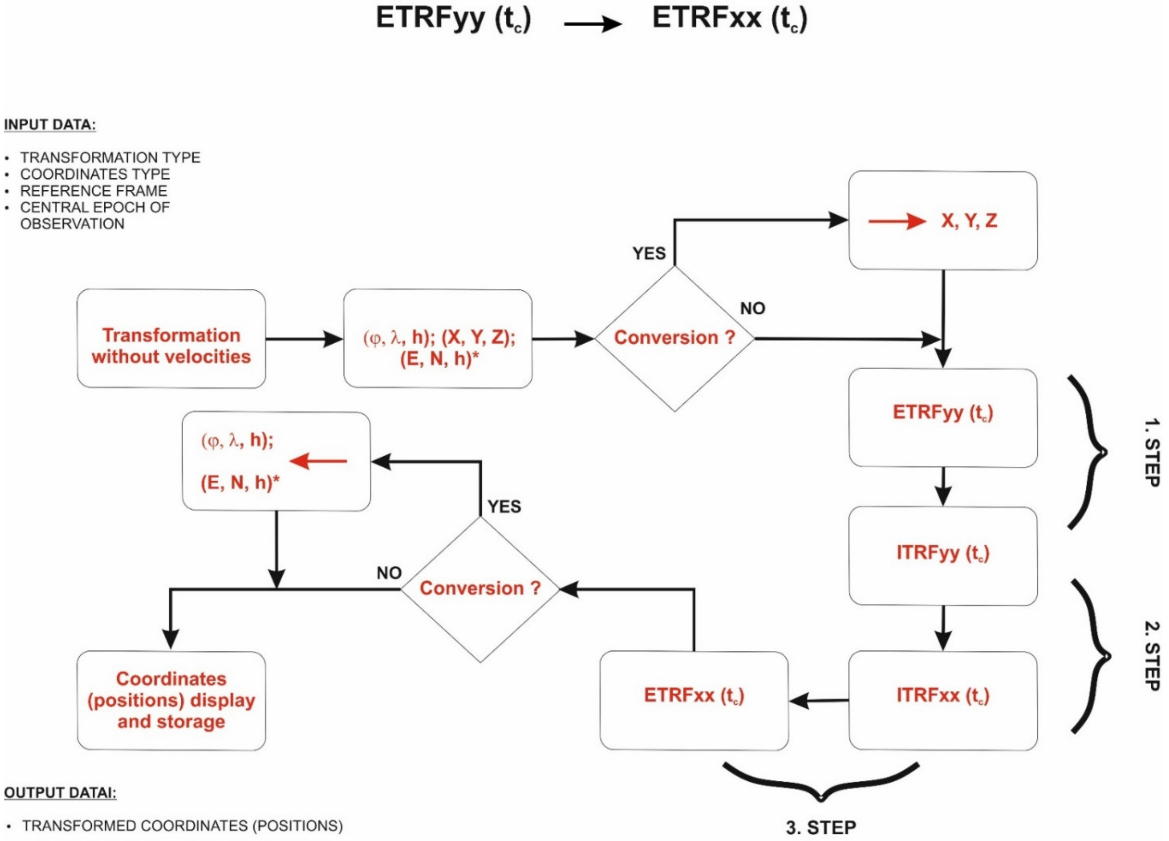
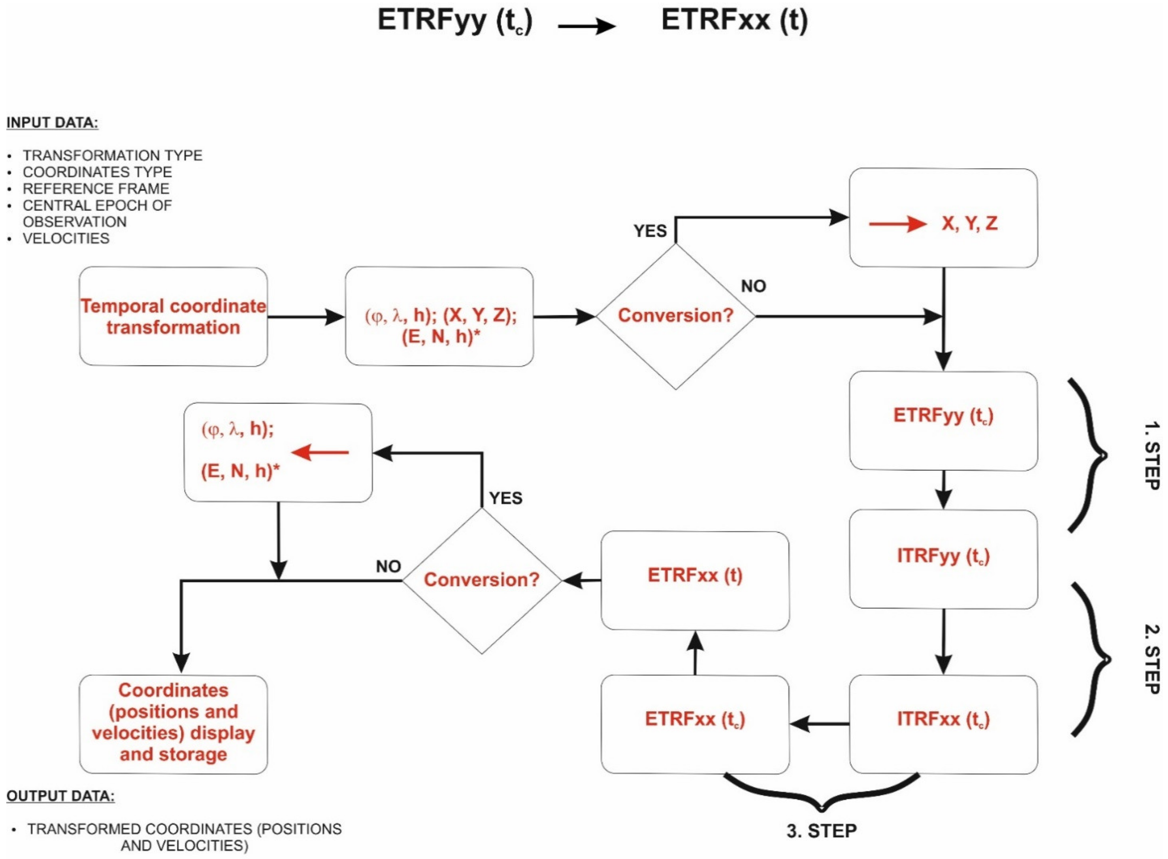
Scheme 1 and
Scheme 2 show the transformation workflows of the TranSAB application.
Scheme 1 relates to the transformation between two different ETRS89 realizations where velocities were not included, hereby denoted as ETRF
yy and ETRF
xx, while
Scheme 2 shows the corresponding transformation but with velocities included in the transformation model.
6. Implementing the Application in the Real World—Temporal Coordinate Transformation
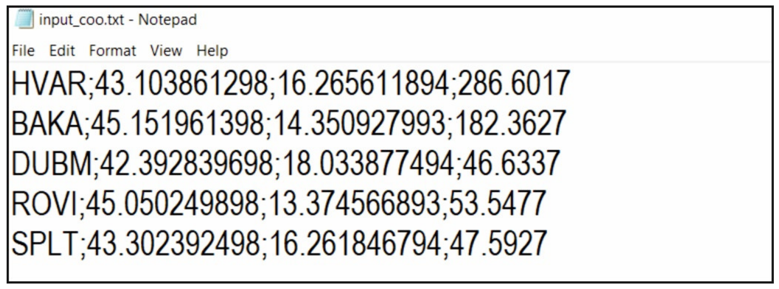
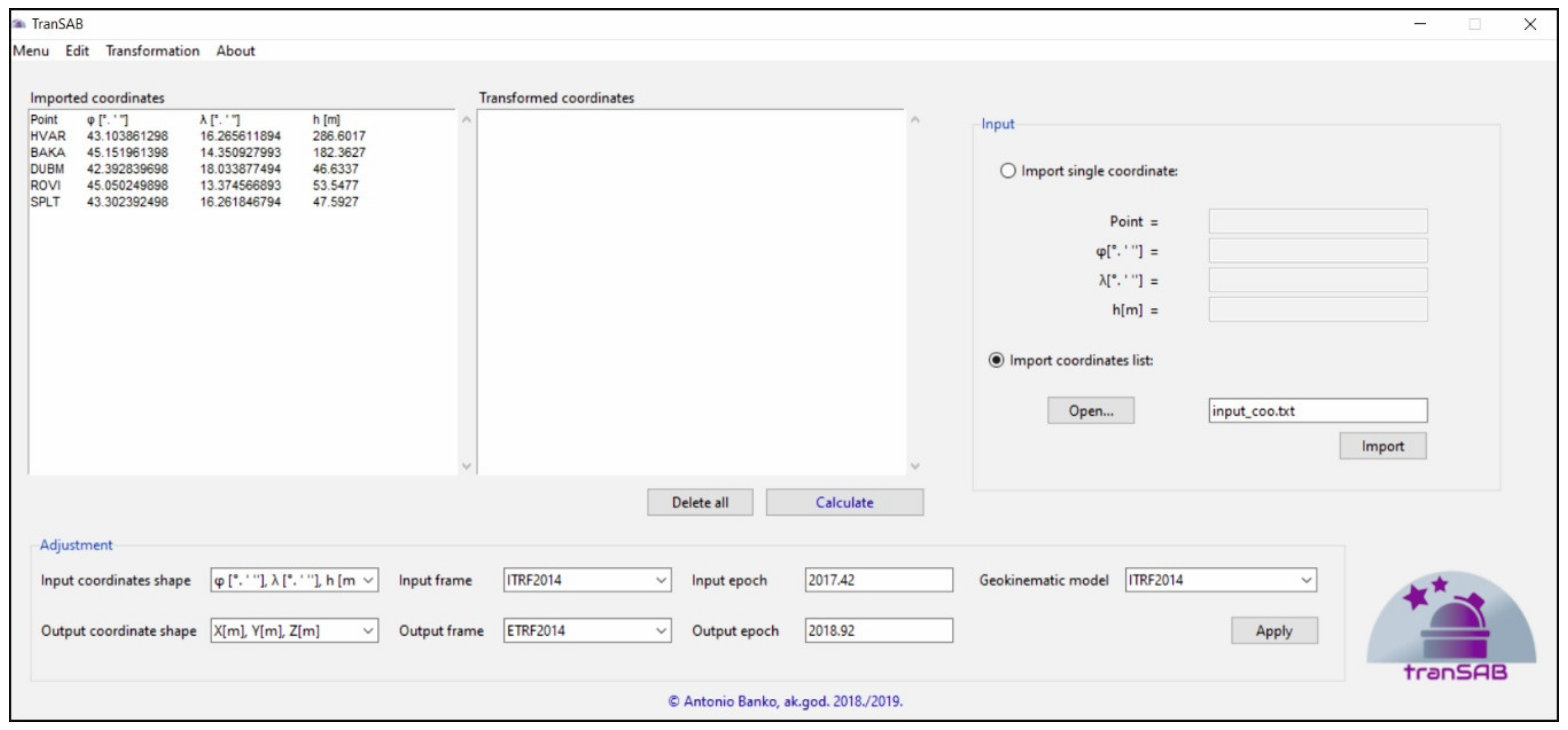
Suppose that the user has a set of ellipsoidal coordinates in the degrees, minutes, and seconds (DMS) format, as displayed in
Figure 3. The coordinates are given regarding the latest frame of the ITRS ITRF2014 and are expressed at the epoch 2017.42. The desired output is Cartesian coordinates in the ETRF2014 solution and at the epoch 2018.92. According to the tooltip mentioned in
Section 4, velocities are calculated using an associated kinematic model—ITRF2014. The input and output parameters are shown in
Figure 3.
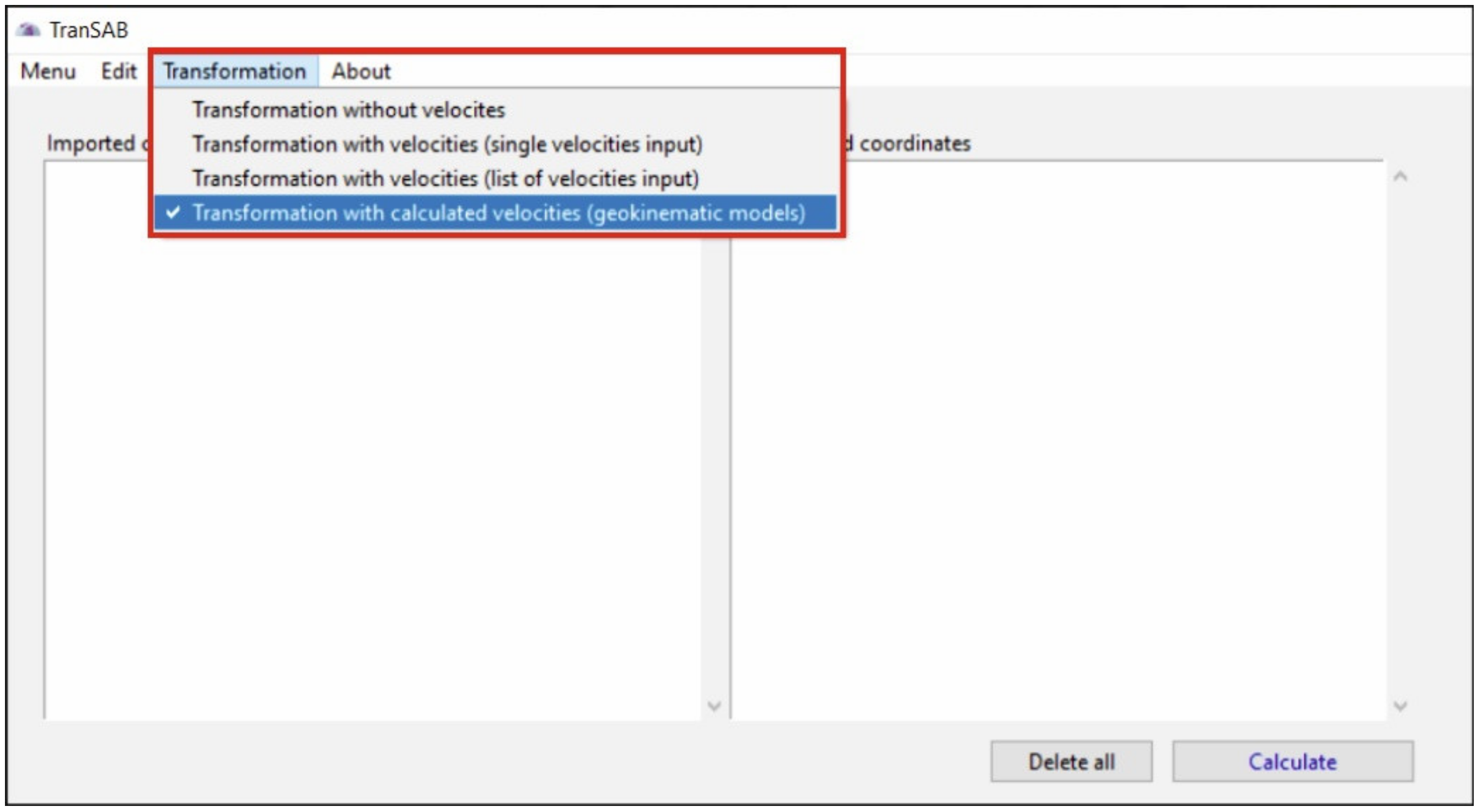
Figure 4 displays a drop-down menu with the possible transformation types. The first option relates to transformation regardless of tectonic plates; hence, without velocities. The second and third options refer to transformation with velocities where the velocities are manually inserted (as a single point or as a data set). The last option, the one chosen in
Figure 3, relates to transformation with velocities where the velocities are computed with the use of kinematic models. If the user chooses the last option, then this transformation model should be selected before the parameters are set and coordinates imported.
After selecting the transformation type, the user can access parameter adjustment and coordinate insertion.
Figure 5 shows the GUI of TranSAB where the parameters are set, and coordinates imported, following the above-mentioned approach.
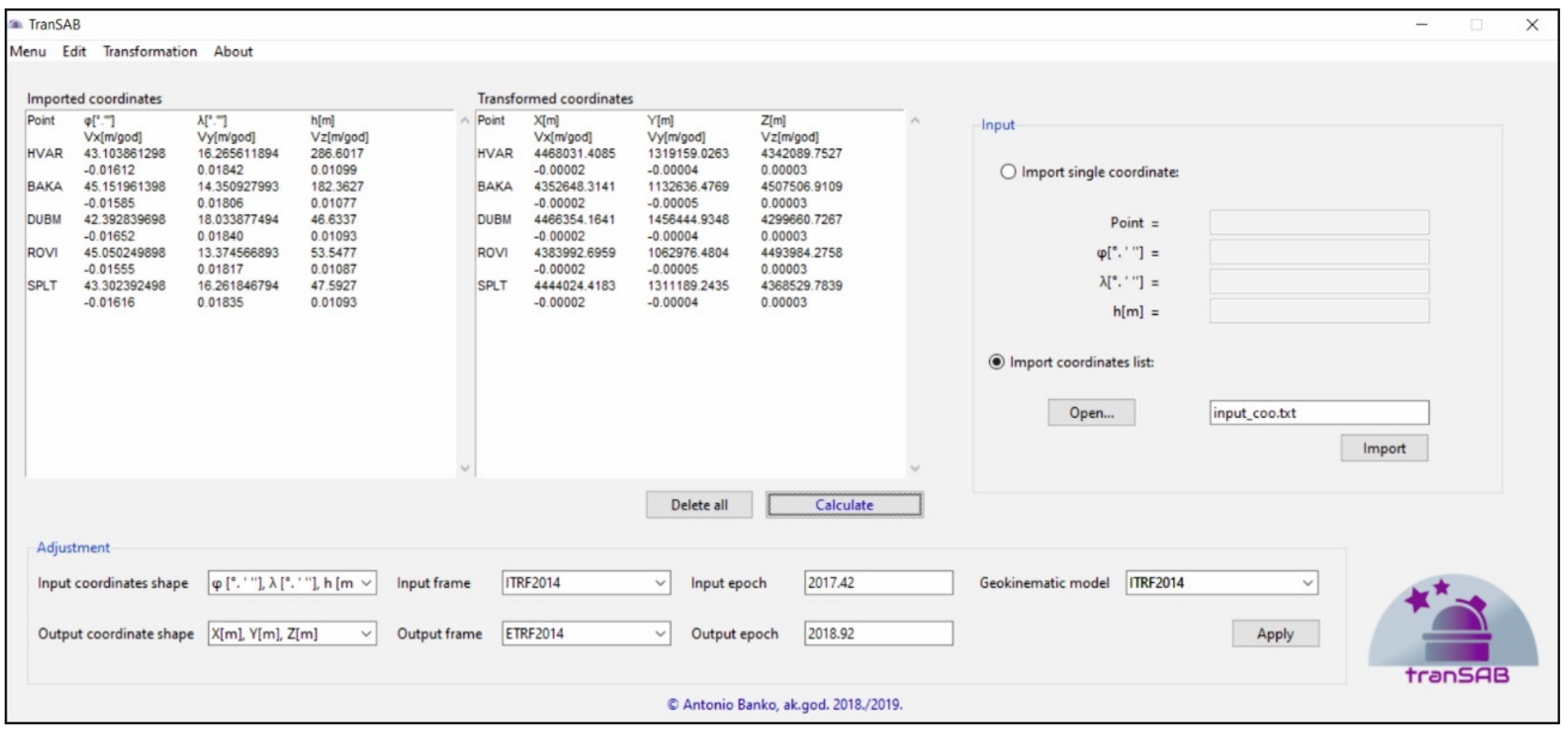
It can be noticed in
Figure 6 that the velocities are displayed under the section ‘imported coordinates’. These velocities refer to those calculated with the use of the kinematic model (in this case, the kinematic model is the ITRF2014 plate motion model) before the transformation occurs. The section ‘transformed coordinates’ in
Figure 6 displays the positions (Cartesian coordinates (
X, Y, Z) with unit meters) and velocities (
VX, VY,
VZ with unit meters per year) of the stations calculated (transformed) using the formulas, procedures, and recommendations given in this paper.
After the transformation is completed, TranSAB offers users an option to save the computed coordinates in *.txt format for further processes or other purposes.
7. Discussion
In addition to its intuitive, easy-to-handle, and user-friendly GUI, the TranSAB application offers an all-in-one solution. An all-in-one solution implies the possibility of temporal coordinate transformations which existing programs and services do not offer. Station velocities are computed with the use of NNR kinematic models of the Eurasian tectonic plate, which are already implemented in the transformation model. Another possibility to calculate station velocities can be realized by applying the appropriate kinematic model of the Adriatic microplate (as a part of the Eurasian tectonic plate) obtained from our own research [
8,
9,
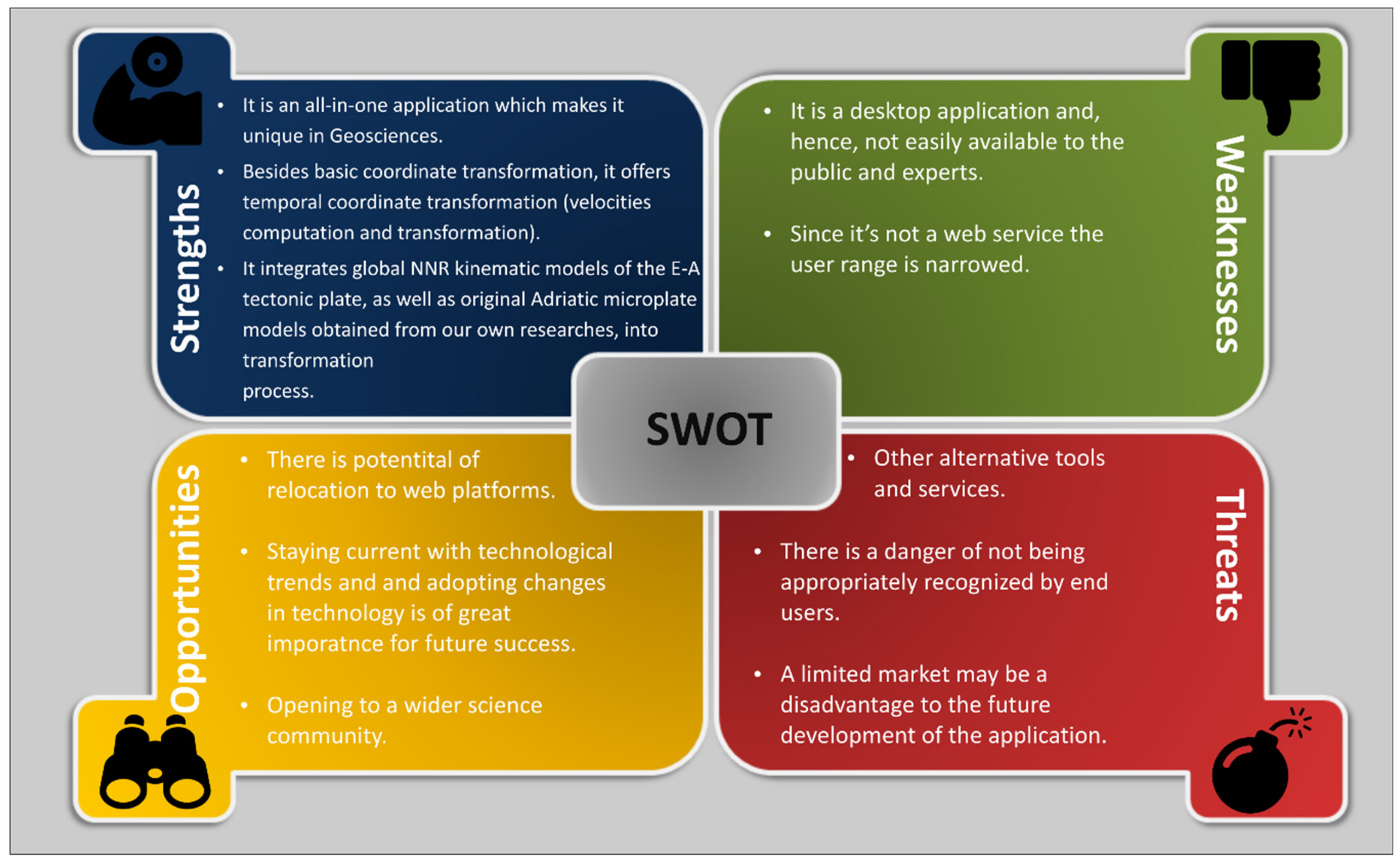
10]. On the other hand, since this is a desktop application and not a web service, the user range and availability to others are limited, not to mention that a great obstacle to application development can be alternative tools and services (i.e., competitors), which are already well known. Users not accepting the application and its features may slow down its development and limit the market for its use as too. Nonetheless, there is considerable potential to bypass these barriers. For instance, relocating the application to web platforms and being current with technological trends, as well as properly anticipating and adopting technological changes, can attract a bigger audience and expand the user community.
Figure 7 presents the SWOT (strengths, weaknesses, opportunities, threats) analysis.
Constant developments in satellite-based measuring techniques are progressively making a more significant impact on the “three pillars” of geodesy. Consequently, more accurate reference frames and kinematic models are being defined. Due to the new and more accurate reference frame realizations, the necessity for coordinate transformation between them is growing more each day. Moreover, the fact that points on the Earth’s surface are not stationary but are a function of time due to tectonic plate motions increases the need for faster and simpler temporal coordinate transformation. TranSAB, a standalone desktop application, offers solutions for the above-mentioned problems. The application was developed following general recommendations given by EUREF TN and utilizing the EUREF online tool for coordinate transformation (position and velocity). Particular emphasis was placed on unifying coordinate transformations, where EUREF TN served as a source to adopt transformation protocols, together with global NNR kinematic models of lithospheric plate motions.
The TranSAB application was made with the intent to meet the needs of all those who are dealing with the processing and adjustment of GNSS measurements and the (temporal) transformation of obtained results between two different reference frames. It represents a unique solution for coordinate transformation in geodesy and geoinformatics because it utilizes EUREF coordinate transformation procedures and annual coordinate shifts due to plate tectonics by selecting the appropriate NNR kinematic model to compute station velocities by their coordinates. It is a user-friendly application with an intuitive GUI, intended for all users who are dealing with processed GNSS data, as well as those who want to express spatial coordinates in an appropriate coordinate reference frame. Creating an all-in-one standalone application was the first step because it was easier than creating a web application; the second step would be to provide free access to all interested parties and the wider scientific community; and the third step, should there be enough interest, would certainly be a web application. We are of the belief that the development of the TranSAB application is of great significance for geoscience and beyond.


