Visual Exposure of Rock Outcrops in the Context of a Forest Disease Outbreak Simulation Based on a Canopy Height Model and Spectral Information Acquired by an Unmanned Aerial Vehicle


Abstract
:1. Introduction
1.1. Aim of the Study
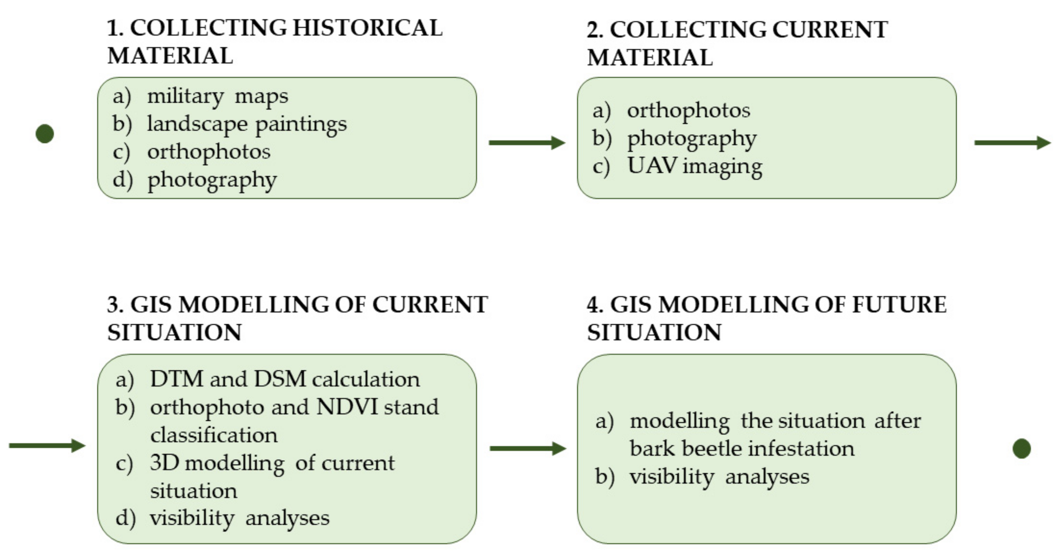
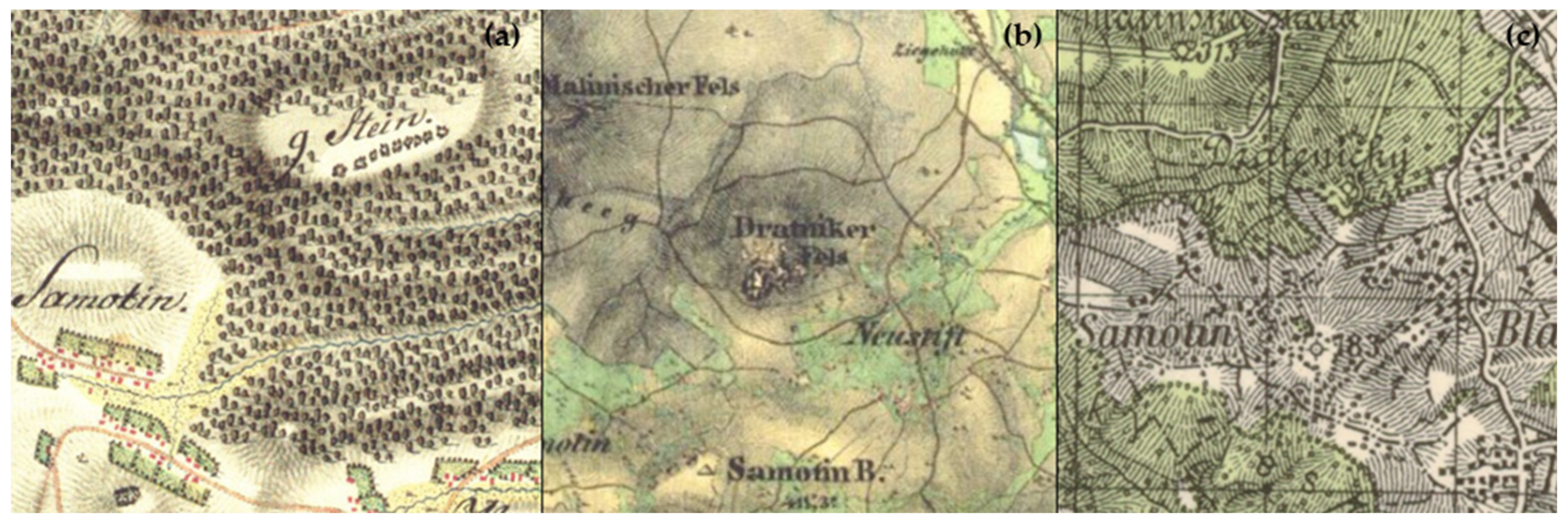
- landscape painting and historical maps,
- historical and current photographs and orthophoto, and
- unmanned aerial vehicle (UAV) remote-sensing data and digital terrain and surface models.
1.2. Landscape Painting
1.3. Remote Sensing
2. Materials and Methods
2.1. Protected Landscape Area Žďárské vrchy
2.1.1. Geology and Geomorphology
2.1.2. Flora and Fauna
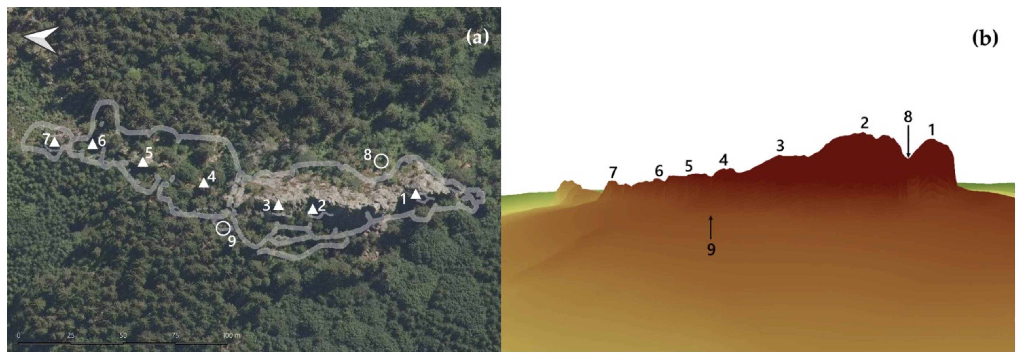
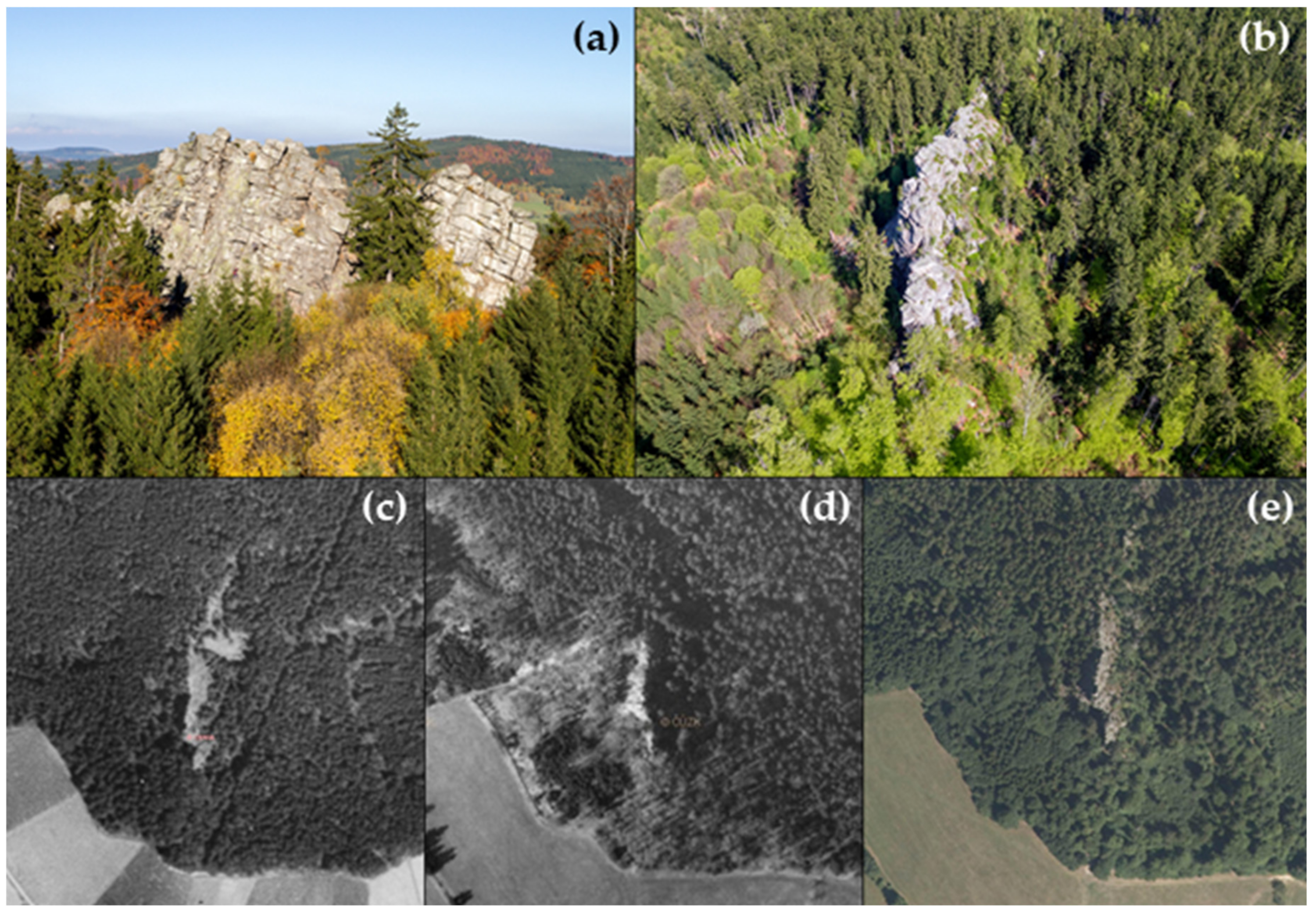
2.1.3. Drátenická Skála
2.2. Baseline of the Study
2.3. Methodological Approach
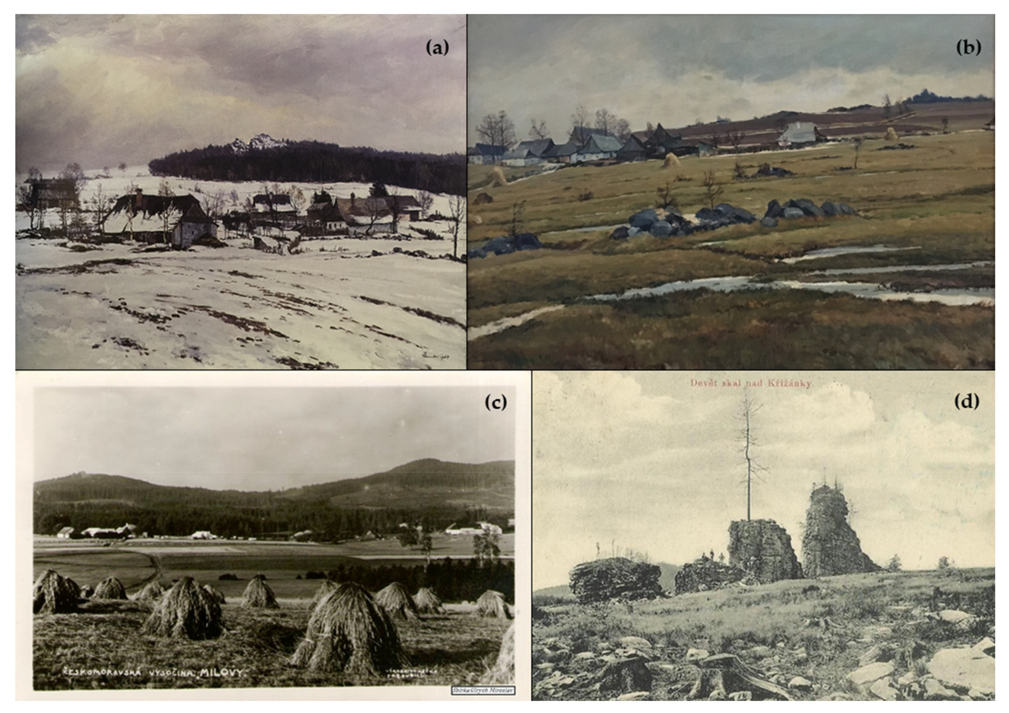
- Josef Jambor, Zima pod Drátníkovou skálou, 1954;
- Josef Jambor Horní Blatiny, 1946; and
- Milan Zimmermann, Dráteníky u Samotína, 2005.
3. Results and Discussion
3.1. Historic and Artistic Material
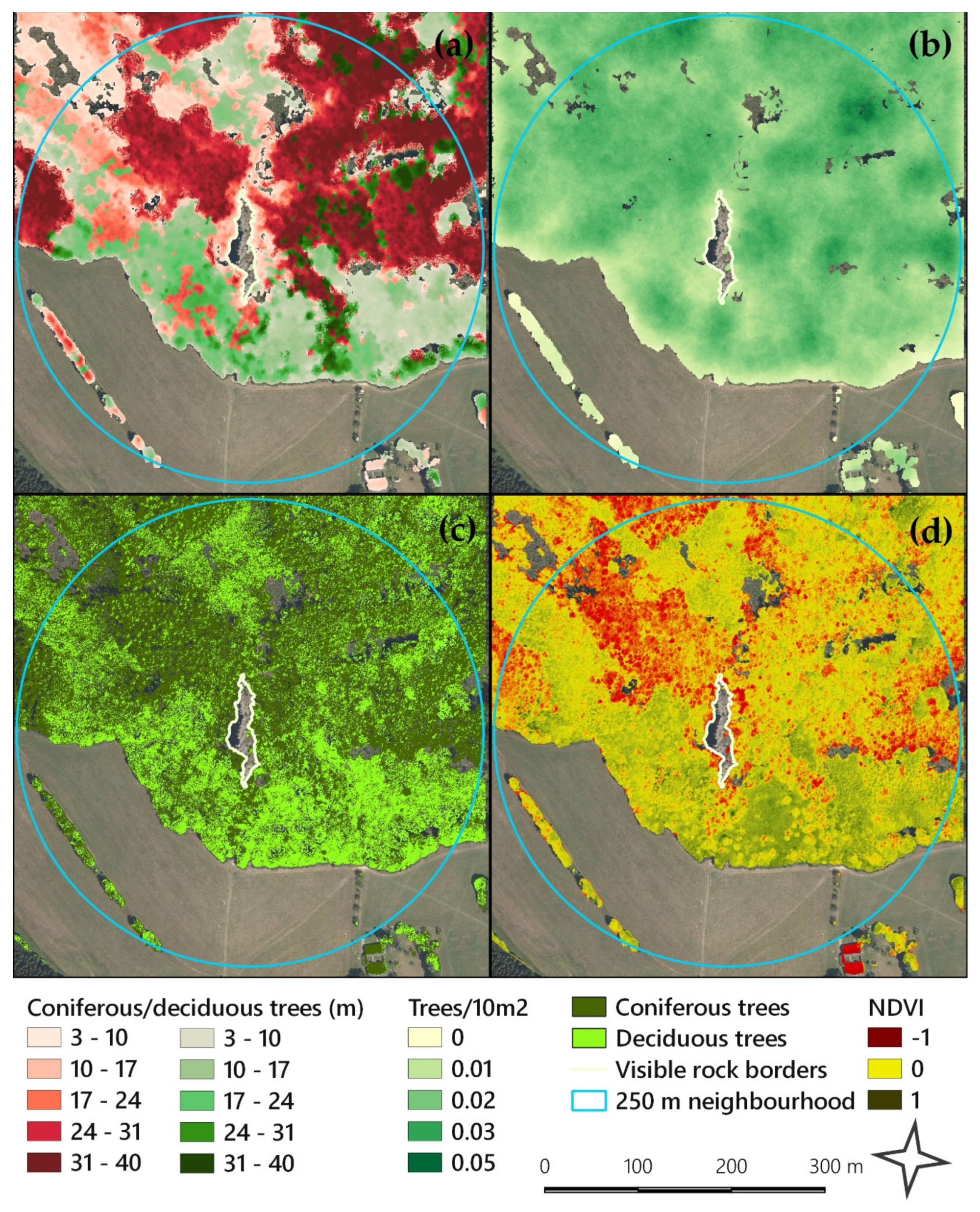
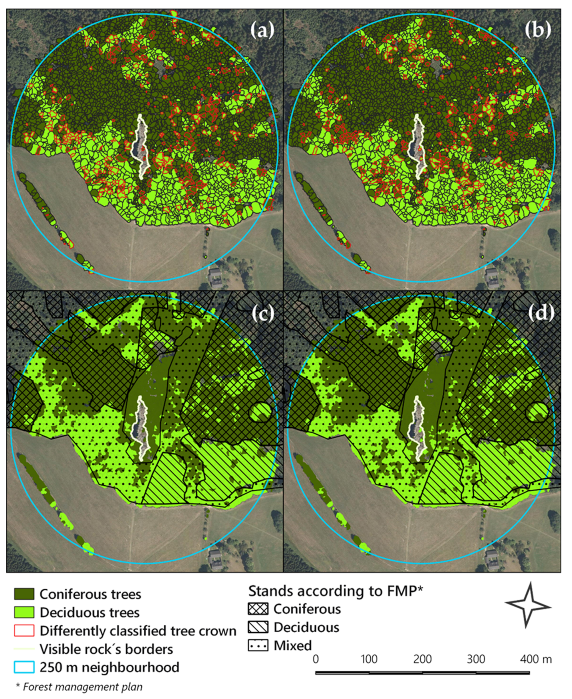
3.2. GIS Modelling
4. Conclusions
Author Contributions
Funding
Acknowledgments
Conflicts of Interest
References
- Cartwright, J. Ecological islands: Conserving biodiversity hotspots in a changing climate. Front. Ecol. Environ. 2019, 17, 331–340. [Google Scholar] [CrossRef] [Green Version]
- Peñaloza-Bojacá, G.F.; de Oliviera, A.B.; Teixeira Araújo, C.A.; Fantecelle, B.L.; dos Santos, D.N.; Maciel-Silva, A. Bryophytes on Brazilian ironstone outcrops: Diversity, environmental filtering, and conservation implications. Flora 2018, 238, 162–174. [Google Scholar] [CrossRef]
- Speziale, K.L.; Ezcurra, C. Rock outcrops as potential biodiversity refugia under climate change in North Patagonia. Plant Ecol. Divers. 2015, 8, 353–361. [Google Scholar] [CrossRef]
- Do Carmo, F.F.; Jacobi, C.M. Diversity and plant trait-soil relationships among rock outcrops in the Brazilian Atlantic rainforest. Plant Soil 2016, 403, 7–20. [Google Scholar] [CrossRef]
- Balková, M.; Bajer, A. An Unconventional Promotion of Rock Outcrops in Žďárské Vrchy PLA Using Remote Sensing. In Public Recreation and Landscape Protection—With Nature Hand in Hand! Conference Proceeding, 1st ed.; Mendel University in Brno: Brno-sever-Černá Pole, Czech Republic, 2018; pp. 23–27. ISBN 978-80-7509-550-3. Available online: http://www.utok.cz/sites/default/files/data/USERS/u24/RaOP%202018_WEB_1_0.pdf (accessed on 10 August 2019).
- Henshillwood, C.S.; d´Errico, F.; van Niekerk, K.L.; Dayet, L.; Queffelec, A.; Pollarolo, L. An abstract drawing from the 73,000-year-old levels at Blombos Cave, South Africa. Nature 2018, 562, 115–118. [Google Scholar] [CrossRef]
- Clottes, J. The ´three Cs´: Fresh avenues towards European Paleolithic Art. In The Archeoloy of Rock Art; Chippindale, C., Tacon, P.S.C., Eds.; Cambridge University Press: Cambridge, UK, 2018. [Google Scholar]
- Chauvet, J.M.; Brunel Deschamps, E.; Hillaire, C. Dawn of Art: The Chauvet Cave: The Oldest Known Paintings in the World; H.N. Abrams: New York, NY, USA, 1996. [Google Scholar]
- Robb, J. Prehistoric art in Europe: A deep-time social history. Am. Antiq. 2015, 80, 635–654. [Google Scholar] [CrossRef]
- Lacina, J.; Halas, P. Landscape painting in evaluation of changes in landscape. J. Landsc. Ecol. 2015, 8, 60–68. [Google Scholar] [CrossRef] [Green Version]
- Wehr, A.; Lohr, U. Airborne laser scanning—An introduction and overview. ISPRS J. Photogramm. Remote Sens. 1999, 54, 68–82. [Google Scholar] [CrossRef]
- Baltsavias, E.P. Airborne laser scanning: Existing systems and firms and other resources. ISPRS J. Photogramm. Remote Sens. 1999, 54, 164–198. [Google Scholar] [CrossRef]
- Brázdil, K. Technická Zpráva k Digitálnímu Modelu Reliéfu 5. Generace (DMR 5G) (Technical Report of the Digital Terrain Model of the Czech Republic of the 5th Generation (DTM5G)); State Administration of Land Surveying and Cadastre: Prague, Czech Republic, 2012. [Google Scholar]
- Mikita, T. Hodnocení přesnosti digitálního modelu povrchu 1. generace v lesních porostech a možnosti využití dat v lesnické praxis (Evaluation of accuracy of the digital surface model of the 1st generation in forest stands and possibilities of data usage in forestry practice). Geod. Kartogr. Obz. 2014, 12, 317–323. [Google Scholar]
- Mikita, T.; Cibulka, M.; Janata, P. Hodnocení přesnosti digitálních modelů reliéfu 4. A 5. generace v lesních porostech (Evaluation of accuracy of the digital terrain models of the 4th and 5th generation in forest stands and possibilities of data usage in forestry practice). Geod. Kartogr. Obz. 2013, 4, 76–85. [Google Scholar]
- Iglhaut, J.; Cabo, C.; Puliti, S.; Piermattei, L.; O’Connor, J.; Rosette, J. Structure from motion photogrammetry in forestry: A review. Curr. For. Rep. 2019, 5, 155–168. [Google Scholar] [CrossRef] [Green Version]
- Goodbody, T.R.H.; Coops, N.C.; White, J.C. Digital aerial photogrammetry for updating area-based forest inventories: A review of opportunities, challenges, and future directions. Curr. For. Rep. 2019, 5, 55–75. [Google Scholar] [CrossRef] [Green Version]
- Michez, A.; Piégay, H.; Lisein, J.; Claessens, H.; Lejeune, P. Classification of riparian forest species and health condition using multi-temporal and hyperspatial imagery from unmanned aerial system. Environ. Monit. Assess. 2016, 188, 146. [Google Scholar] [CrossRef] [PubMed] [Green Version]
- Brovkina, O.; Cienciala, E.; Surový, P.; Janata, P. Unmanned aerial vehicles (UAV) for assessment of qualitative classification of Norway spruce in temperate forest stands. Geo Spat. Inf. Sci. 2018, 21, 12–20. [Google Scholar] [CrossRef] [Green Version]
- Puliti, S.; Ørka, H.O.; Gobakken, T.; Naesset, E. Inventory of small forest areas using an unmanned aerial system. Remote Sens. 2015, 7, 9632–9654. [Google Scholar] [CrossRef] [Green Version]
- Tuominen, S.; Balazs, A.; Saari, H.; Pölönen, I.; Sarkeala, J.; Viitala, R. Unmanned aerial system imagery and photogrammetric canopy height data in area-based estimation of forest variables. Silva Fenn. 2015, 49, 1348. [Google Scholar] [CrossRef] [Green Version]
- Mikita, T.; Janata, P.; Surový, P. Forest stand inventory based on combined aerial and terrestrial close-range photogrammetry. Forests 2016, 7, 165. [Google Scholar] [CrossRef] [Green Version]
- Næsset, E.; Økland, T. Estimating tree height and tree crown properties using airborne scanning laser in a boreal nature reserve. Remote Sens. Environ. 2002, 79, 105–115. [Google Scholar] [CrossRef]
- Hyyppä, J.; Inkinen, M. Detecting and estimating attributes for single trees using laser scanner. Photogramm. J. Finl. 1999, 16, 27–42. [Google Scholar]
- Guerra-Hernández, J.; Cosenza, D.N.; Rodriguez, L.C.E.; Silva, M.; Tomé, M.; Díaz-Varela, R.A.; González-Ferreiro, E. Comparison of ALS- and UAV(SfM)- derived high-density point clouds for individual tree detection in Eucalyptus plantations. Int. J. Remote Sens. 2018, 39, 5211–5235. [Google Scholar] [CrossRef]
- Mohan, M.; Silva, C.; Klauberg, C.; Jat, P.; Catts, G.; Cardil, A.; Hudak, A.T.; Dia, M. Individual tree detection from unmanned aerial vehicle (UAV) derived canopy height model in an open canopy mixed conifer forest. Forests 2017, 8, 340. [Google Scholar] [CrossRef] [Green Version]
- Nevalainen, O.; Honkavaara, E.; Tuominen, S.; Viljanen, N.; Hakala, T.; Yu, X.; Hyyppä, J.; Saari, H.; Pölönen, I.; Imai, N.N.; et al. Individual tree detection and classification with UAVbased photogrammetric point clouds and hyperspectral imaging. Remote Sens. 2017, 9, 185. [Google Scholar] [CrossRef] [Green Version]
- Lisein, J.; Pierrot-Deseilligny, M.; Bonnet, S.; Lejeune, P. A photogrammetric workflow for the creation of a forest canopy height model from small unmanned aerial system imagery. Forests 2013, 4, 922–944. [Google Scholar] [CrossRef] [Green Version]
- Stone, C.; Mohammed, C. Application of remote sensing technologies for assessing planted forests damaged by insect pests and fungal pathogens: A review. Curr. For. Rep. 2017, 3, 75–92. [Google Scholar] [CrossRef]
- Näsi, R.; Honkavaara, E.; Lyytikäinen-Saarenmaa, P.; Blomqvist, M.; Litkey, P.; Hakala, T.; Viljanen, N.; Kantola, T.; Tanhuanpää, T.; Holopainen, M. Using UAV-based photogrammetry and hyperspectral imaging for mapping bark beetle damage at tree-level. Remote Sens. 2015, 7, 15467–15493. [Google Scholar] [CrossRef] [Green Version]
- Minařík, R.; Langhammer, J. Use of a multispectral Uav photogrammetry for detection and tracking of forest disturbance dynamics. Int Arch Photogramm. Remote Sens. Spat. Inf. Sci. 2016, XLI-B8, 711–718. [Google Scholar] [CrossRef] [Green Version]
- Dash, J.P.; Watt, M.S.; Pearse, G.D.; Heaphy, M.; Dungey, H.S. Assessing very high resolution UAV imagery for monitoring forest health during a simulated disease outbreak. ISPRS J. Photogramm. Remote Sens. 2017, 131, 1–14. [Google Scholar] [CrossRef]
- Mikita, T.; Klimánek, M.; Cibulka, M. Hodnocení metod interpolace dat leteckého laserového skenování pro detekci stromů a měřená jejich výšek (Evaluation of Airborne Laser Scanning data interpolation methods for tree detection and height measurement). Zprávy Lesn. Výzkumu 2013, 58, 99–106. [Google Scholar]
- Zhao, B.; Wu, J.; Yang, F.; Pilz, J.; Zhang, D. A novel approach for extraction of Gaoshanhe-Group outcrops using Landsat Operational Land Imager (OLI) data in the heavily loess-covered Baoji District, Western China. Ore Geol. Rev. 2019, 108, 88–100. [Google Scholar] [CrossRef]
- Chesley, J.T.; Leier, A.L.; White, S.; Torres, R. Using unmanned aerial vehicles and structure-from-motion photogrammetry to characterize sedimentary outcrops: An example from the Morrison Formation, Utah, USA. Sediment. Geol. 2017, 354, 1–8. [Google Scholar] [CrossRef]
- Mezghani, M.M.; Fallatah, M.I.; AbuBshait, A.A. From drone-based remote sensing to digital outcrop modeling: Integrated workflow for quantitative outcrop interpretation. J. Remote Sens. GIS 2018, 7, 1000237. [Google Scholar] [CrossRef]
- Blistan, P.; Kovanič, Ľ.; Zelizňaková, V.; Palková, J. Using UAV photogrammetry to document rock outcrops. Acta Monast. Slov. 2016, 2, 154–161. [Google Scholar]
- Burton-Johnson, A.; Black, M.; Fretwell, P.; Kaluza-Gilbert, J. An automated methodology for differentiating rock from snow, clouds and sea in Antarctica from Landsat 8 imagery: A new rock outcrop map and area estimation for the entire Antarctic continent. Cryosphere 2016, 10, 1665–1677. [Google Scholar] [CrossRef] [Green Version]
- Caravaca, G.; Le Mouélic, S.; Mangold, N.; L’Haridon, J.; Le Deit, L.; Massé, M. 3D digital outcrop model reconstruction of the Kimberley outcrop (Gale crater, Mars) and its integration into Virtual Reality for simulated geological analysis. Planet. Space Sci. 2020, 182, 104808. [Google Scholar] [CrossRef]
- Mikita, T.; Balková, M.; Bajer, A.; Cibulka, M.; Patočka, Z. Comparison of different remote sensing methods for 3d modeling of small rock outcrops. Sensors 2020, 20, 1663. [Google Scholar] [CrossRef] [Green Version]
- Kirchner, K. Žďárské Vrchy Highland—Geomorphological Landscape in the Top Part of the Bohemian-Moravian Highland with the Unique Crystalline Rocks Forms. In Landscapes and Landforms of the Czech Republic; Pánek, T., Hradecký, J., Eds.; Springer: Cham, Switzerland, 2016; pp. 221–231. ISBN 978-3-319-27536-9. [Google Scholar] [CrossRef]
- Rozbory Chráněné krajinné oblasti Žďárské vrchy (Analyzes of the Žďárské vrchy Protected Landscape Area), Nature Conservation Agency of the Czech Republic. Available online: https://drusop.nature.cz/ost/archiv/plany_pece/index.php?frame&ID=23662 (accessed on 5 August 2019).
- Čech, L. Chráněná území ČR, svazek VII.—Jihlavsko (Protected areas of the Czech Republic, Volume VII.—Jihlavsko); Nature Conservation Agency of the Czech Republic: Prague, Czech Republic, 2002; p. 528. [Google Scholar]
- Plán Péče o Chráněnou Krajinnou Oblast Žďárské Vrchy na Období 2011–2020 (Management Plan of Žďárské Vrchy Protected Landscape Area for the Period 2011–2020), Nature Conservation Agency of the Czech Republic. Available online: https://drusop.nature.cz/ost/archiv/plany_pece/index.php?frame&ID=23662 (accessed on 5 August 2019).
- Demek, J.; Mackovčin, P. Zeměpisný lexikon ČR—Hory a nížiny (Geographical Lexicon of the Czech Republic—Mountains and Lowlands); Agency of the Czech Republic: Prague, Czech Republic, 2006; p. 588. [Google Scholar]
- Hanžl, P. Geology of the Žďárské Vrchy Area: A Review, Travaux Géophysiques; Institute of Geophysics, Czech Academy of Sciences: Prague, Czech Republic, 2011; Volume 40, p. 24. [Google Scholar]
- Melichar, R.; Buriánek, D.; Břízová, E.; Buriánková, K.; Čurda, J.; Fürych, V.; Hanžl, P.; Kirchner, K.; Lysenko, V.; Mrnková, J.; et al. Vysvětlivky k Základní Geologické Mapě České Republiky 1:25000 (Explanatory Notes to Basic Geological Map of the Czech Republic 1:25000), Sheet 24-111 Sněžné; Czech Geological Survey: Prague, Czech Republic, 2004; p. 58. [Google Scholar]
- Bajer, A.; Kirchner, K.; Kubalíková, L. Geodiversity values as a basis for geosite and geomorphosite assessment: A case study from Žďárské vrchy Highland. In Central Europe Area in View of Current Geography. Proceedings of 23rd Central European Conference, 1st ed.; Masaryk University in Brno: Brno, Czech Republic, 2016; pp. 56–69. ISBN 978-80-210-8313-4. [Google Scholar]
- Gray, M. Geodiversity: Valuing and Conserving Abiotic Nature; John Wiley: Chichester, UK, 2004; p. 434. [Google Scholar]
- Kubešová, S.; Novotný, I.; Sutorý, K. Inventarizační Průzkum Cévnatých Rostlin A Mechorostů (Inventory Survey of Vascular Plants And Bryophytes) Bílá Skála, Černá Skála, Devět Skal, Drátenická Skála, Lisovská Skála, Malinská Skála, Milovské Perničky, Pasecká Skála, Rybenské Perničky, Vlčí Kámen; Moravian museum: Brno, Czech Republic, 2006; p. 55. [Google Scholar]
- Chytrý, M.; Kučera, T.; Kočí, M. Katalog Biotopů České Republiky (Catalog of Habitats of the Czech Republic); Agency of the Czech Republic: Prague, Czech Republic, 2001; p. 220. [Google Scholar]
- Drvotová, M. Měkkýši (Mollusca) Žďárských Vrchů. (Molluscs (Mollusca) of the Žďárské vrchy Mts.), Parnassia; Agency of the Czech Republic, Administration of PLA Žďárské vrchy: Žďár and Sázavou, Czech Republic, 2008; Volume 3, p. 79. [Google Scholar]
- Svatoň, J. Pavouci (Araneae) Žďárských vrchů. Faunisticko-ekologická studie. (Spiders (Araneae) of the Žďárské vrchy Mts. Faunistic and ecology study), Parnassia; Agency of the Czech Republic, Administration of PLA Žďárské vrchy: Žďár and Sázavou, Czech Republic, 2006; Volume 1, p. 100. [Google Scholar]
- Kirchner, K.; Roštínský, P. Geomorfologická inventarizace vybraných skalních útvarů v centrální části CHKO Žďárské vrchy (Geomorphological inventory of selected rock formations in the central part of the PLA Žďárské vrchy). In Proceedings of the Faculty of Science, University of Ostrava, Geography, Geology; University of Ostrava: Ostrava, Czech Republic, 2007; Volume 237, pp. 48–64. [Google Scholar]
- Bajer, A.; Hlaváč, V.; Kirchner, K.; Kubalíková, L. Za Skalními Útvary CHKO Žďárské Vrchy (To the Rock Formations of the PLA Žďárské Vrchy); Mendel University in Brno, Institute of Geonics, Czech Academy of Science: Brno, Czech Republic, 2014; p. 88. ISBN 978-80-7375-959-9. [Google Scholar]
- Orthophoto of the Czech Republic. WMS Service. State Administration of Land Surveying and Cadastre: Prague, Czech Republic, 2018. Available online: http://geoportal.cuzk.cz/WMS_ORTOFOTO_PUB/WMService.aspx (accessed on 15 June 2019).
- Digital Terrain Model of the Czech Republic of the 5th Generation; State Administration of Land Surveying and Cadastre: Prague, Czech Republic, 2013.
- Doležal, F.; Trefulka, F. Žďárské vrchy. Průvodce po Horolezeckých Terénech Vysočiny (Guide to Climbing Terrains of the Vysočina Highlands); Physical Education Unity Vysočina: Žďár nad Sázavou, Czech Republic, 2006; p. 106. [Google Scholar]
- Lacina, J.; Halas, P. Vodní nádrže a jejich krajina ve výtvarném umění (Water reservoirs and their landscape in fine art). Vodohospod. Tech. Ekon. Inf. 2017, 59, 31–39. [Google Scholar]
- Doubek, J. Odlesnění skal na Žďársku aneb jak se rodí kompromisy (Deforestation of rocks in Žďár region, or how compromises are born). Lesnická Práce 2013, 92, 16–18. [Google Scholar]
- Hlaváč, V. Znovu k záměru “odlesnění skal” na Žďársku (Again to the intention of “rocks deforestation” in the Žďár region). Lesn. Pr. 2014, 93, 34–35. [Google Scholar]
- Pike, D.A.; Webb, J.K.; Shine, R. Removing forest canopy cover restores a reptile assemblage. Ecol. Appl. 2011, 21, 274–280. [Google Scholar] [CrossRef]
- Michael, D.R.; Lindenmayer, D.B.; Cunningham, R.B. Managing rock outcrops to improve biodiversity conservation in Australian agricultural landscapes. Ecol. Manag. Restor. 2010, 11, 43–50. [Google Scholar] [CrossRef]
- Plán Péče o Přírodní Památku Malínská Skála na Období 2016–2025 (Management plan of Malínská skála natural monument for the period 2016–2025). Nature Conservation Agency of the Czech Republic. Available online: https://drusop.nature.cz/ost/archiv/plany_pece/index.php?frame&ID=26881 (accessed on 6 August 2019).
- Plán Péče o Přírodní Památku Bílá Skála na Období 2016–2025 (Management plan of Bílá skála natural monument for the period 2016–2025). Nature Conservation Agency of the Czech Republic. Available online: https://drusop.nature.cz/ost/archiv/plany_pece/index.php?frame&ID=26880 (accessed on 6 August 2019).
- Plán Péče o Přírodní Památku Černá Skála na Období 2016–2025 (Management plan of Černá skála natural monument for the period 2016–2025). Nature Conservation Agency of the Czech Republic. Available online: https://drusop.nature.cz/ost/archiv/plany_pece/index.php?frame&ID=26809 (accessed on 6 August 2019).
- Plán Péče o Přírodní Památku Devět Skal na Období 2016–2025 (Management plan of Devět skal natural monument for the period 2016–2025). Nature Conservation Agency of the Czech Republic. Available online: https://drusop.nature.cz/ost/archiv/plany_pece/index.php?frame&ID=26805 (accessed on 6 August 2019).
- Plán Péče o Přírodní Památku Drátenická Skála na Období 2016–2025 (Management plan of Drátenická skála natural monument for the period 2016–2025). Nature Conservation Agency of the Czech Republic. Available online: https://drusop.nature.cz/ost/archiv/plany_pece/index.php?frame&ID=26806 (accessed on 29 June 2019).
- Fotohistorie (Photohistory). Available online: http://www.fotohistorie.cz/Default.aspx (accessed on 2 June 2019).
- 1st Military Survey, Section No. 15; Austrian State Archive/Military Archive: Vienna, Austria, 2003.
- 2nd Military Survey, Section No. W_6_II; Austrian State Archive/Military Archive: Archive/Military Archive, 2006.
- 3rd Military Survey, Section No. 4156; Nature Conservation Agency of the Czech Republic: Prague, Czech Republic, 2009.
- Oldmaps. Laboratory of Geoinformatics, Jan Evangelista Purkyně University in Ústí nad Labem. Available online: http://oldmaps.geolab.cz (accessed on 7 June 2019).
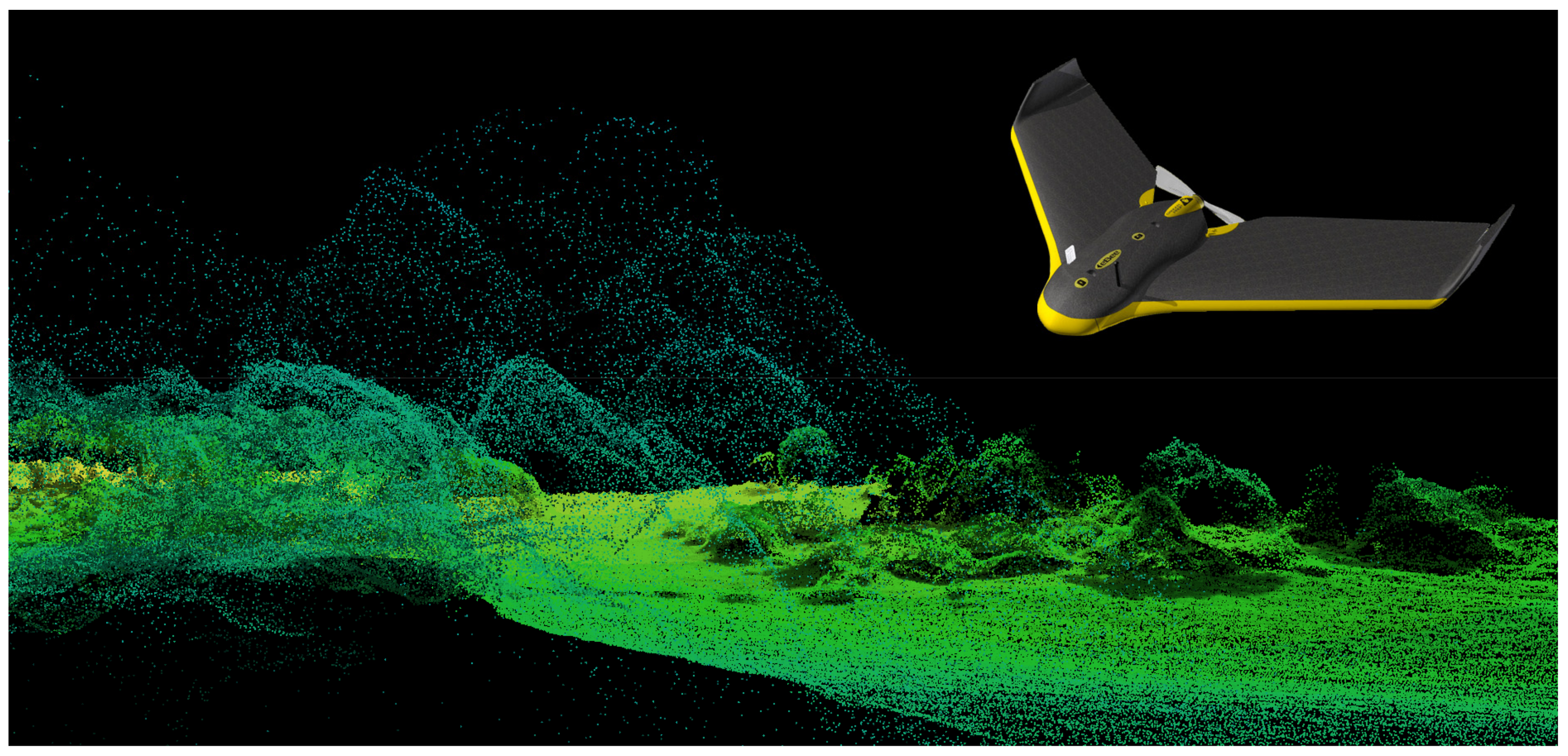
- SenseFly Parrot Group. Available online: https://www.sensefly.com/expand/ (accessed on 16 August 2019).
- Edson, C.B. Light Detection And Ranging (Lidar): What We Can and Cannot See in The Forest For The Trees; UMI Dissertation Publishing, Oregon State University: Corvallis, OR, USA, 2011; p. 277. [Google Scholar]
- Weir, J.; Herring, D. Measuring Vegetation (NDVI and EVI); NASA Earth Observatory: Washington, DC, USA, 2000; Available online: https://earthobservatory.nasa.gov/features/MeasuringVegetation/measuring_vegetation_2.php (accessed on 10 August 2019).
- Geoportal. Forests of the Czech Republic, State-Owned Company. Available online: https://geoportal.lesycr.cz/itc/?serverconf=default&wmcid=882 (accessed on 22 August 2019).


| Number of Trees | Area (m2) | Density (Trees/1000 m2) | Part of Stands Area (%) | Average Height (m) | ||
|---|---|---|---|---|---|---|
| Orthophoto | Deciduous stand | 1233 | 59 543 | 20.7 | 42.7 | 16.5 |
| Coniferous stand | 2125 | 79 696 | 26.6 | 57.3 | 25.8 | |
| NDVI | Deciduous stand | 1172 | 58 975 | 19.8 | 42.4 | 16.8 |
| Coniferous stand | 2186 | 84 871 | 25.8 | 57.6 | 25.4 | |
| Total | 3 358 | 139.249 | 25.8 | 100.0 | 22.2 |
| Stands According to FSM * | Number of Trees | Part of Whole Area/Stands (%) | ||
|---|---|---|---|---|
| Orthophoto Classification | NDVI Classification | Orthophoto Classification | NDVI Classification | |
| Coniferous | 1246 | 1246 | 37.0 | 37.0 |
| Con. | 1006 | 1065 | 80.1 | 85.4 |
| Dec. | 240 | 214 | 19.9 | 14.6 |
| Deciduous | 402 | 402 | 12.4 | 12.4 |
| Con. | 111 | 83 | 25.2 | 19.1 |
| Dec. | 291 | 319 | 75.8 | 80.9 |
| Mixed | 1710 | 1710 | 50.6 | 50.6 |
| Con. | 1008 | 1038 | 53.1 | 55 |
| Dec. | 702 | 672 | 46.9 | 45 |
| Sum | 3358 | 3358 | 100.0 | 100.0 |
| Class | Coniferous Trees | Deciduous Trees | Total | User’s Accuracy |
|---|---|---|---|---|
| Coniferous trees | 95 | 7 | 102 | 0.9314 |
| Deciduous trees | 10 | 88 | 98 | 0.8980 |
| Total | 105 | 95 | 200 | |
| Producer’s accuracy | 0.9048 | 0.9263 | 0.9150 | |
| Kappa | 0.8298 |
| Class | Coniferous Trees | Deciduous Trees | Total | User’s Accuracy |
|---|---|---|---|---|
| Coniferous trees | 85 | 17 | 102 | 0.8333 |
| Deciduous trees | 20 | 78 | 98 | 0.7959 |
| Total | 105 | 95 | 200 | |
| Producer’s accuracy | 0.8095 | 0.8211 | 0.8150 | |
| Kappa | 0.6296 |
| Places in Relation to Peak Visibility | Situation in 2019 | Situation without Coniferous | ||
|---|---|---|---|---|
| Area (m2) | % of the Area | Area (m2) | % of the Area | |
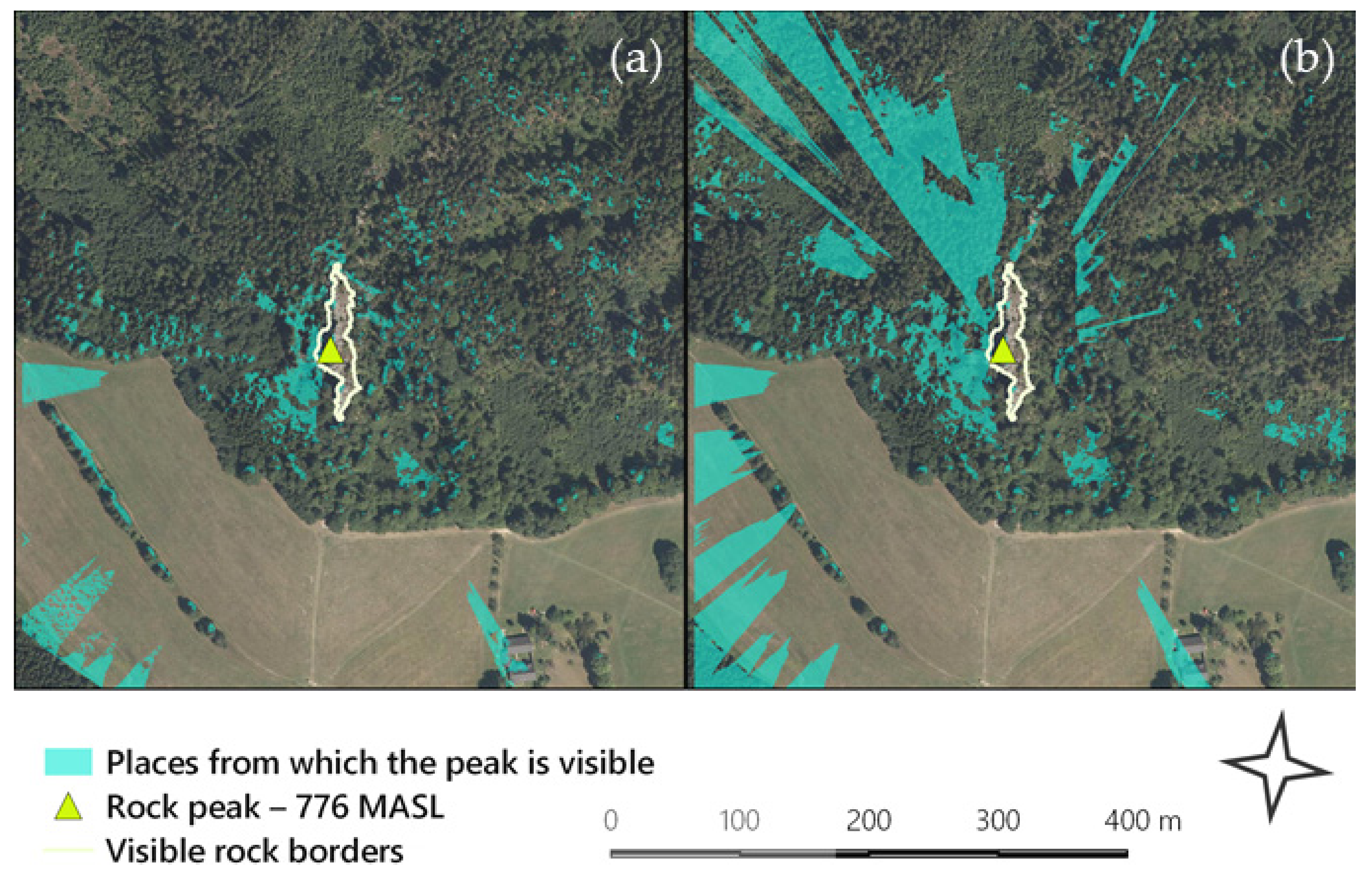
| Visible | 13,216.80 | 3.90 | 48,388.50 | 14.40 |
| Invisible | 322,584.20 | 96.10 | 287,412.50 | 85.60 |
| Whole area | 335,801.00 | 100.00 | 335,801.00 | 100.00 |
© 2020 by the authors. Licensee MDPI, Basel, Switzerland. This article is an open access article distributed under the terms and conditions of the Creative Commons Attribution (CC BY) license (http://creativecommons.org/licenses/by/4.0/).
Share and Cite
Balková, M.; Bajer, A.; Patočka, Z.; Mikita, T. Visual Exposure of Rock Outcrops in the Context of a Forest Disease Outbreak Simulation Based on a Canopy Height Model and Spectral Information Acquired by an Unmanned Aerial Vehicle. ISPRS Int. J. Geo-Inf. 2020, 9, 325. https://0-doi-org.brum.beds.ac.uk/10.3390/ijgi9050325
Balková M, Bajer A, Patočka Z, Mikita T. Visual Exposure of Rock Outcrops in the Context of a Forest Disease Outbreak Simulation Based on a Canopy Height Model and Spectral Information Acquired by an Unmanned Aerial Vehicle. ISPRS International Journal of Geo-Information. 2020; 9(5):325. https://0-doi-org.brum.beds.ac.uk/10.3390/ijgi9050325
Chicago/Turabian StyleBalková, Marie, Aleš Bajer, Zdeněk Patočka, and Tomáš Mikita. 2020. "Visual Exposure of Rock Outcrops in the Context of a Forest Disease Outbreak Simulation Based on a Canopy Height Model and Spectral Information Acquired by an Unmanned Aerial Vehicle" ISPRS International Journal of Geo-Information 9, no. 5: 325. https://0-doi-org.brum.beds.ac.uk/10.3390/ijgi9050325